A Plastic Network Approach to Model Calving Glacier Advance and Retreat

1. Introduction

The global sea level rise contribution from land ice is large and growing (Rignot et al., 2011; van den Broeke et al., 2016). Much of the increase in the land ice contribution to sea level rise comes from the dynamic response of marine-terminating glaciers, including those draining the Greenland and Antarctic Ice Sheets (Church et al., 2013; Straneo et al., 2013; Vaughan et al., 2013). Where glaciers drain the large ice sheets, there is often a transition from laterally unconfined ice (width ≳ 10² km) to flow through narrow fjords (width ~10 km or smaller). For example, most of the 199 widest Greenland outlet glaciers studied by Murray et al. (2015) do not exceed 3 km in width, and many smaller glaciers less than one kilometer in width are excluded from consideration. Where tidewater glaciers drain alpine ice fields, as in coastal Alaska, the ice flux through the terminus may come from tens or hundreds of tributary branches upstream. The largest glaciers with the greatest potential contribution to sea level rise also have the most tributary branches—more than 400 in the case of Hubbard Glacier, Alaska (Kienholz et al., 2015).

The relatively small scale and large number of outlet glaciers and tributaries present a challenge to effective ice sheet modeling: the fine resolution required to capture small-glacier dynamics is prohibitively expensive to apply in full-Stokes models of entire ice sheets. Adaptive mesh refinement (AMR) has been applied in some models, e.g., BISICLES (Cornford et al., 2013), as a first step toward addressing this challenge. However, the finest-resolution cells (~500 m) in AMR grids are generally those nearest the grounding line, potentially leaving upstream tributaries of width ~1 km and smaller unresolved. By contrast, simplified centerline models applied to individual glaciers may use grid spacing of < 10 m over the entire glacier length, but such models often ignore tributary branches entirely.

In Ultee and Bassis (2016), we extended the perfect plastic approximation of Nye (1951, 1952, 1953) to a centerline model of tidewater glaciers that self-consistently predicts terminus advance and retreat forced with upstream elevation change. We now generalize this model to account for the intersection of networks of tributaries. Our plastic model is well-suited to this problem because the condition for intersections is straightforward: ice thickness H must match at intersection points between branches. Here, we describe the model's application to intersecting glacier networks through four case studies, including glaciers from both Alaska and Greenland. We also discuss two alternative forcing methods that could bring glacier-wide mass balance—and its changes due to climate—directly into the model.

As illustrative cases, we choose four large, well-studied glaciers: Jakobshavn Isbræ and Helheim Glacier, Greenland, and Columbia and Hubbard Glaciers, Alaska. These glaciers were chosen based on their diversity of behavior and because of the (relatively) abundant data available. For example, geometry of these glaciers varies from Jakobshavn's single major channel to Hubbard's more than 400 mountain tributaries. Moreover, in recent decades Columbia and Jakobshavn have been undergoing sustained retreat (Krimmel, 2001; Joughin et al., 2004, 2012, 2014; O'Neel et al., 2005; McNabb et al., 2012), Hubbard has been advancing (Trabant et al., 2003; Ritchie et al., 2008) and Helheim has experienced both advance and retreat episodes (Howat et al., 2005, 2010; Murray et al., 2010), providing tests of our model's ability to resolve calving dynamics in a range of environments. Further, with the case studies selected here we go beyond the work of Ultee and Bassis (2016) to show that the model can reproduce patterns of retreat and advance in both Greenland and Alaska and that the model can be used to analyze glaciers with more than one branch.

2. Methods

Our method extends the perfect plastic approximation of Nye (1951, 1952, 1953) to calving glaciers with a network of tributaries. The perfect plastic approximation corresponds to the assumption that glacier ice is perched at a yield strength. Applying the approximation to a glacier centerline as in Ultee and Bassis (2016), we obtain an equation for the surface elevation profile along the centerline:

$\begin{array}{ll}|h-b|\frac{\partial h}{\partial x}=\frac{{\tau }_{\mathrm{\text{b}}}}{{\rho }_{\mathrm{\text{i}}}g},& (1)\end{array}$

where h is glacier surface elevation, b bed elevation, ${\rho }_{\mathrm{\text{i}}}=920{\mathrm{\text{kg m}}}^{-3}$ the density of glacier ice, g = 9.81 m s⁻² the acceleration due to gravity, and τ_b the basal yield strength.

At the calving front, we require that tractions balance across the ice-water interface, i.e.,

$\begin{array}{ll}{\displaystyle {\int }_{b(x)}^{h(x)}}{\sigma }_{xx}\mathrm{\text{ d}}z={\displaystyle {\int }_{b(x)}^0}-{\rho }_{w}gz\mathrm{\text{ d}}z,& (2)\end{array}$

with ${\rho }_{\mathrm{\text{w}}}=1020{\mathrm{\text{ kg m}}}^{-3}$ the density of sea water. We also require that the ice at the terminus is at the yield strength of ice, τ_y, and integrating as in Ultee and Bassis (2016) provides a corresponding condition on the ice thickness at the terminus:

$\begin{array}{ll}{H}_{\mathrm{\text{terminus}}}=2\frac{{\tau }_{\mathrm{\text{y}}}}{{\rho }_{\mathrm{\text{i}}}g}+\sqrt{\frac{{\rho }_{\mathrm{\text{w}}}{D}^2}{{\rho }_i}+2\frac{{\tau }_{\mathrm{\text{y}}}}{{\rho }_{\mathrm{\text{i}}}g}}& (3)\end{array}$

where

$\begin{array}{ll}D=\{\begin{array}{cc}\left|b(x)\right|& \mathrm{\text{for }}b(x)<0\\ 0\hfill & \mathrm{\text{for }}b(x)\ge 0\end{array}& (4)\end{array}$

represents water depth. For a given terminus position, our model uses Equations (1) and (3) to construct the surface elevation profile along the glacier centerline with a self-consistent terminus position.

A general plastic model admits two yield strengths: that of the bed, τ_b, and that of the ice, here called τ_y. Generally speaking, τ_b ≤ τ_y. When the glacier substrate is weaker than the glacier ice, stress at the calving front (Equation 3) is limited by the yield strength of ice, and basal stress (Equation 1) is limited by the lower yield strength of the bed. The especially simple solution we present here assumes τ_b = τ_y, which may not be realistic but has shown promising results when applied to Columbia Glacier (Ultee and Bassis, 2016). τ_y thus becomes our single adjustable parameter.

This simple model may be run with a constant yield strength, or with a Coulomb yield criterion:

$\begin{array}{rcl}{\tau }_{\mathrm{\text{y}}}={\tau }_0+\mu N,& \mathrm{\text{where }}N=({\rho }_{\mathrm{\text{i}}}gH-{\rho }_{\mathrm{\text{w}}}gD)& (5)\end{array}$

with μ a constant cohesion coefficient, H = h − b the ice thickness, other terms as above, and τ₀ replacing τ_y as the directly adjustable yield parameter. N in Equation (5) represents an effective pressure at the glacier bed, such that basal substrates below sea level can be assumed saturated and promoting faster flow (through a weaker bed and/or more deformation in the adjacent layer of ice). Basal water pressure beneath real glaciers is affected by hydrological factors such as variable meltwater flux and evolution of the basal drainage network, but accounting for such effects is beyond the scope of this simple model. In all four case studies presented here, we keep μ = 0.01 constant to avoid excessive “tuning.” This value was chosen to reflect a Mohr-Coulomb condition with low friction angle—as would be found for soft marine sediments near tidewater glacier termini—and consistent with the laboratory estimates of Cohen et al. (2005).

To apply our one-dimensional centerline model to a network of glacier tributaries, we define the network of centerlines, identify an appropriate value of the yield strength τ_y for the glacier in question, and simulate upstream thinning/thickening over time.

2.1. Define Network Centerlines

Each centerline comprises a sequence of point coordinates. For relatively simple tributary networks, we manually select centerlines from maps of glacier thickness and bed topography. We save the lists of point coordinates and note which are points of intersection between branches. For general cases, it is more practical to extract point coordinates from automatically-generated sets of centerlines such as those created by Machguth and Huss (2014) or Kienholz et al. (2014). With coordinate sequence in hand, we generate a set of evenly-spaced points from the (common) terminus to the head of each glacier branch and we re-express the points of each line in terms of arc length. Expressing the lines in terms of arc length allows a continuous representation of input quantities along each line, allowing model resolution to be adjusted.

2.2. Find Best-Fit Yield Strength

Our model rheology depends on a single adjustable parameter: the yield strength τ_y. Note once again that, though a general plastic model might include separate yield strengths for the glacier bed and glacier ice, τ_b and τ_y, respectively, we assume here that τ_b = τ_y.

Where observed surface elevation profiles are available, we can find the best-fit value for yield strength τ_y (or τ₀ of Equation 5) by minimizing model mismatch with observation. We minimize model misfit only along the main branch, where observations are likely to be higher-quality, testing a range of values of τ_y. We quantify the mismatch with observation using the coefficient of variation of the root-mean-square error, CV_RMS. We take the value of τ_y corresponding to minimum CV_RMS to be the best-fit yield strength, and we apply the same best-fit τ_y to all branches of a given glacier.

For glaciers lacking observations of surface elevation, such as those that have retreated significantly from a less-well-documented initial state, a best-guess value of τ_y may be used instead. Laboratory and field observations indicate that τ_y should be approximately 50–300 kPa (O'Neel et al., 2005; Cuffey and Paterson, 2010), with lower values for soft, flat beds and higher values for hard, steep beds.

2.3. Simulate Advance/Retreat over Time

Using our best-fit or best-guess yield strength, we generate a reference profile along each glacier branch corresponding to an initial terminus position. For the plastic model, terminus retreat corresponds to upstream thinning and advance to thickening. We select an upstream point along the reference profile, ideally a point with good observations available for multiple years, where we will apply changes in ice thickness. We first simulate main branch thinning/thickening as described in Ultee and Bassis (2016), finding the terminus position satisfying Equation 3 for each new glacier profile. Because all tributaries share a common terminus, we use the terminus position identified by the main branch profile and step the plastic model upstream into the tributaries from there. Thus, we generate a consistent set of branch profiles, which by definition agree at the points of intersection, for each time step.

2.4. Numerical Considerations

We discretize Equation 1 with an Euler forward step. The model is fast and can be run with small grid spacing; in the following case studies, grid spacing ranges from 1–5 m to ensure negligible numerical error. Our results are robust and insensitive even to order-of-magnitude increases in grid spacing. We enforce our boundary condition of matching ice thickness at tributary branching points in the model initialization, stepping the model upstream into the tributaries from a common trunk where ice thickness agrees by definition. For more details of our numerical implementation, see Ultee and Bassis (2016).

3. Case Studies

To demonstrate the application of the network method, we now turn to four case studies, arranged in order of increasing complexity. The case studies include calving glaciers in both Alaska and Greenland, with networks ranging from the very simple single branch of Jakobshavn Isbræ to the highly complex Hubbard Glacier network of more than 400 branches (of which we treat eight). Each case illustrates a different capability of the model: matching average retreat based on relatively sparse data, reproducing more detailed retreat including a network split, simulating retreat and readvance without adjusting model settings, and matching a well-studied terminus advance with a forcing fit to observations. In the final case study, we illustrate the application of the model to automatically generated networks of centerlines, dramatically improving the scalability of this approach for large and complex networks of calving glaciers.

3.1. Jakobshavn Isbræ, Greenland—1 Centerline

Jakobshavn Isbræ is the fastest-flowing glacier currently known, with summer flow speeds near the terminus reaching 16 km a⁻¹ (Joughin et al., 2014). It drains approximately 7% of the Greenland Ice Sheet by volume (Joughin et al., 2004; Csatho et al., 2008) and is a substantial contributor to global sea level rise: nearly 1 mm between 2000 and 2011 (Joughin et al., 2014; Howat et al., 2011). A CReSIS level 3 data product (CReSIS, 2016b) provides gridded ice thickness, surface elevation, and ice-bottom elevation for Jakobshavn Isbræ. The CReSIS product is a composite of data collected between 2006 and 2014, with ice bottom reconstructed by kriging of radar lines. Because Jakobshavn lost its floating ice tongue before the period of the CReSIS product (2006–2014), we assume that the terminus is grounded and that ice-bottom elevation corresponds to bed topography everywhere. Three intersecting troughs are visible in the bed topography, but we consider only the 60 kilometers closest to the terminus, common to all three branches. Thus, we begin our investigation with the simplest possible network geometry: a single centerline. Figure 1 shows the selected centerline on a map of Jakobshavn bed topography.

FIGURE 1

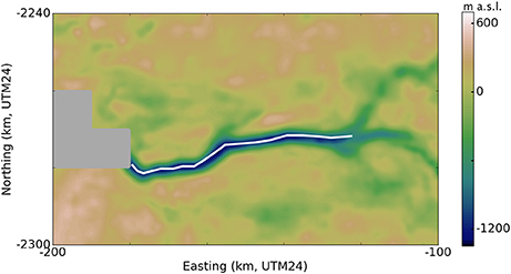
Figure 1. CReSIS 2006–2014 composite bed topography of Jakobshavn Isbræ, with hand-selected centerline (white) for terminal 60 km. Note the dark gray area of no data immediately in front of the terminus.

According to the CReSIS data, our centerline terminates (reaches the end of available data) in ice more than 1400 m thick, grounded more than 1100 m below sea level. If this were the true terminus, it would imply an ice cliff 314 m above the water line—much larger than observations suggest (Joughin et al., 2004, 2014; Csatho et al., 2008). For such a cliff to be stable, the yield strength of ice would have to be more than 3.5 MPa, which is an order of magnitude larger than the values we would expect from observation and our previous work (see O'Neel et al., 2005; Bassis and Walker, 2012; Bassis and Jacobs, 2013; Ultee and Bassis, 2016). Thus, we suspect that the seaward end of our centerline does not represent a true “terminus” with ice-water interface, making it unsuitable for our optimization procedure initialized with the balance thickness (Equation 3). We instead initialize with the observed terminal thickness and proceed with optimization upstream, finding the best fit with τ_y = 355 kPa. Figure 2 compares the centerline profile generated by our plastic model with the observed centerline profile from CReSIS data. The plastic model fit to observation is good, with CV_RMS = 3.3%.

FIGURE 2

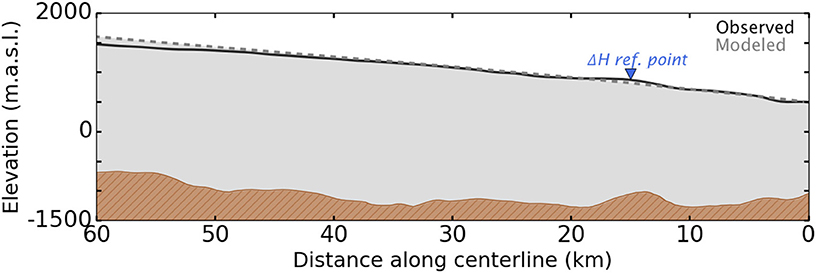
Figure 2. Centerline profiles of Jakobshavn Isbræ: CReSIS composite of surface observations 2006–2014 (black curve) and plastic model with τ_y = 355 kPa (gray dashed curve). Blue marker indicates the upstream reference point where forcing was applied to simulate retreat (see Figure 3).

In recent years, Jakobshavn has thinned and retreated substantially. Using an average thinning rate based on Csatho et al. (2008), we investigate whether the plastic model produces appropriate retreat. Figure 3 shows the simulated change in terminus position with 30 m a⁻¹ thinning applied 15 km upstream from the original terminus (reference point marked in blue in Figure 2). After a few years of thinning without change in terminus position, retreat begins in the third year of the simulation and accelerates to just over 1 km a⁻¹ in years 5–15. Over the entire 15-year period, average retreat rate is 763 m a⁻¹.

FIGURE 3

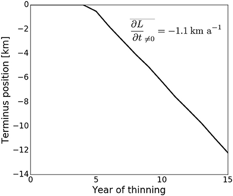
Figure 3. Jakobshavn Isbræ terminus retreat under 15 years of 30 m a⁻¹ upstream thinning. Average retreat rate $\overline{\frac{\partial L}{\partial t}}$ is listed for the years after onset of retreat; compare with rates of 0.83–2.23 km a⁻¹ reported by Csatho et al. (2008) for a similar time period.

Our simulation of the retreat is simplistic, but not unreasonable. Because we initialize from a dataset compositing observations between 2006 and 2014, the onset date of our retreat could be anytime in that range, and comparison with observed retreat is inexact. However, we note that between 1991 and 2006, Csatho et al. (2008) report a 15-year average retreat rate of 830 m a⁻¹, comparable to the 15-year average retreat rate of 763 m a⁻¹ found in our simulation. Further, for the 5-year period 2001–2006, closer to the probable time of our simulated retreat, the average retreat rate reported by Csatho et al. (2008) is 2.23 km a⁻¹, on the order of our retreat rate of 1.1 km a⁻¹ in the years after onset of retreat in the simulation. Our results are of similar magnitude to those reported in Joughin et al. (2004, 2012, 2014) for the early 2000's as well. Though we do not capture the strong seasonal cycling observed at Jakobshavn's terminus (Joughin et al., 2014) under our constant annual upstream thinning, our results are satisfactory for our primary interest in annual- to decadal-scale change.

3.2. Columbia Glacier, Alaska—3 Centerlines

Alaska's Columbia Glacier is among the most well-documented cases of tidewater glacier retreat. The glacier has been monitored by the United States Geologic Survey (USGS) since the early twentieth century, and over the past 35 years it has undergone rapid terminus retreat and upglacier thinning. Datasets available from McNabb et al. (2012) and Krimmel (2001) document the state of Columbia Glacier before and during its recent retreat. McNabb et al. (2012) offers topography and ice thickness reconstructed for 1957 and 2007 from observations, using a mass-conservation algorithm based on Glen's flow law; Krimmel (2001) gives more frequent flightline observations of the glacier surface elevation.

Figure 4 shows the structure of our hand-selected tributary network over Columbia Glacier bed topography. A Coulomb yield criterion with τ₀ = 130 kPa gives the best model fit to observation. Each panel of Figure 5 is an aerial view of the same Columbia Glacier network, illustrating different aspects of the model results. Figure 5A shows glacier surface elevation for plastic steady-state profiles generated with the 1957 terminus position; Figure 5B shows ice thickness for the same profiles; Figure 5C compares the modeled profiles to observation (1957 USGS topographic map, as presented in McNabb et al., 2012). The maximum error is 58% overestimation of ice thickness on parts of the east branch and 44% underestimation of ice thickness on the upper reaches of the main branch, though the percent error in modeled ice thickness is highly spatially variable, as seen in Figure 5C. Overall, the plastic model fit to observed surface elevation as measured by CV_RMS is good along the main and west branches (CV_RMS = 6.2% and 9.5%, respectively) but weaker along the east branch (19.9%). The east branch, where our model tends to overestimate ice thickness by 50% or more, has seldom been directly studied (Krimmel, 2001), although recent radar-sounding and bed-mapping efforts (Rignot et al., 2013; Enderlin et al., 2016) have better constrained the bed topography there and can be applied in future use of our model. We note also that the stretch of the main branch with the poorest fit to observation is the location of a sharp drop in the bedrock, where we might expect problems with the plastic model due to its strong dependence on bed topography.

FIGURE 4

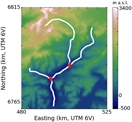
Figure 4. Three branches of Columbia Glacier (white) with reconstructed bed topography from McNabb et al. (2012). Red diamonds mark intersections of the branches.

FIGURE 5

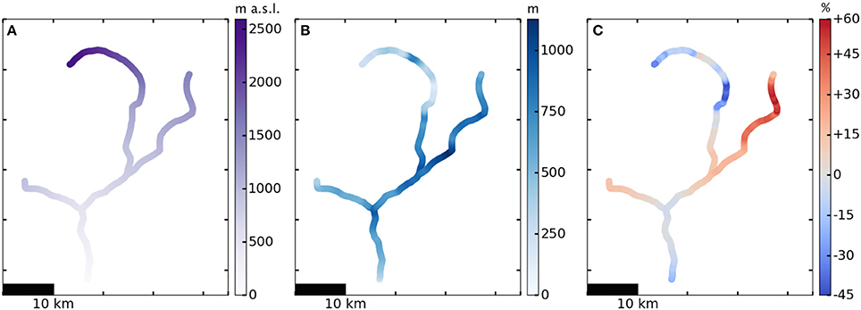
Figure 5. Plastic model with τ_y = 130 kPa + μN applied to a network of three major tributaries of Columbia Glacier, aerial view, 1957. (A) Glacier surface elevation, (B) Ice thickness, (C) Percent error model-observation (McNabb et al., 2012). A positive percent error (red colors in C) corresponds to model overestimation of observed ice thickness, and a negative percent error (blue colors) corresponds to underestimation.

We explore the retreat patterns of Columbia Glacier in detail using a single-branch model in Ultee and Bassis (2016). Here, we apply constant upstream thinning of 8 m a⁻¹ for 25 a, 1982–2007, and show the simulated 2007 state of Columbia Glacier in Figure 6. The color schemes in the two figures have been kept the same (with the exception of the percent error plotted in Figure 6C) to allow for direct comparison. We note that the most pronounced changes occur in the lower reaches of the glacier, including a striking terminus retreat of more than 20 km. Very little change is visible in the upper reaches of the main branch, which agrees with observations of Columbia's dynamics above and below a “hinge point” (an icefall) approximately 40 km upstream from the 1957 terminus (McNabb et al., 2012).

FIGURE 6

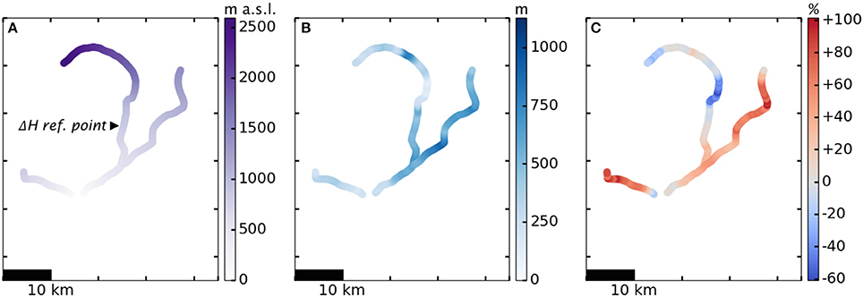
Figure 6. Same panels as Figure 5, simulated for 2007. Black marker indicates upstream location where forcing was applied to simulate retreat. Note the color scales: maintained in (A,B) to facilitate comparison between years, but adjusted in (C) to accommodate the greater error of the model in 2007.

During the dramatic retreat between 1957 and 2007, the terminus of Columbia Glacier reached the intersection point of two branches and eventually split into two calving fronts, shedding icebergs from each branch. That split is visible in Figure 6. Once the terminus retreated upstream of the intersection point, it was necessary to run the model separately on the two smaller networks comprising the single-branch network to the west and the two-branch network to the east. Our model is able to handle this separation of tributaries with little difficulty.

3.3. Helheim Glacier, Greenland—5 Centerlines

Helheim Glacier is another of Greenland's largest outlet glaciers, located along its southeast coast. In recent years, Helheim was observed to thin, retreat, and accelerate, then slow its retreat and begin readvancing (Stearns and Hamilton, 2007; Howat et al., 2010, 2005; Murray et al., 2015). A CReSIS level 3 data product (CReSIS, 2016a) provides gridded ice thickness, surface elevation, and ice bottom elevation for Helheim Glacier. The product we are using is a composite of data collected between 2006 and 2014, with the ice bottom reconstructed by kriging of radar lines.

Figure 7 shows the ice bottom elevation underlying five branches of Helheim Glacier, with hand-selected centerlines for the branches marked in white. We optimize for the yield strength and find that the Coulomb yield criterion with τ₀ = 245 kPa provides the best fit to observation.

FIGURE 7

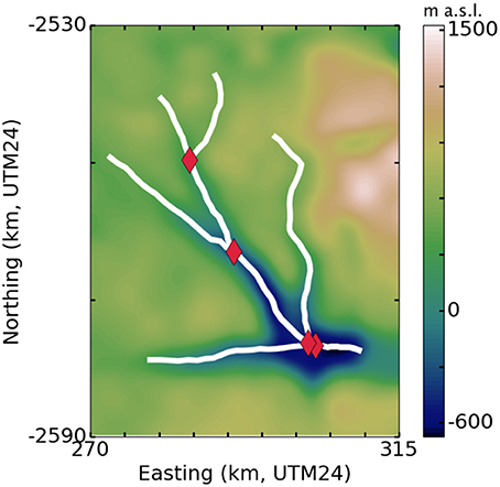
Figure 7. Five branches of Helheim Glacier (white) with CReSIS composite ice bottom elevation from 2006–2014. Red diamonds mark intersections of the branches.

Figure 8, analogous to Figure 5, shows the plastic model applied to the network of five branches of Helheim. The maximum errors are 47.5% overestimation of ice thickness on parts of the easternmost branch and 5.8% underestimation of ice thickness on upstream portions of the two central branches. For four of the five branches studied, the plastic model fit to the CReSIS composite is very good (CV_RMS ≤ 7.9%). For the easternmost branch, the fit is weaker, with CV_RMS = 23.8%. This is likely because the best-fit Coulomb yield strength, τ₀ = 245 kPa, was optimized for the main branch and is too high for the easternmost branch. Running the optimization procedure for each branch individually, we find that the best-fit Coulomb yield strength is between 220 and 250 kPa for all other branches, but only 140 kPa for that easternmost branch. It is possible that ice-dynamical factors unique to that branch, e.g., a different balance of basal/wall drag, affect the optimal yield strength.

FIGURE 8

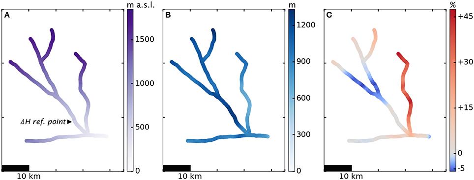
Figure 8. Plastic model with τ_y = 245 kPa + μN applied to network of five major tributaries of Helheim Glacier, aerial view, 2006-2014. (A) Glacier surface elevation, (B) Ice thickness, (C) Percent error model-observation (CReSIS, 2016a).

Given Helheim's recent pattern of retreat and readvance, we now investigate whether the plastic model can produce retreat and readvance within a single simulation. We fit a sinusoidal function to the upstream surface elevation changes reported in Murray et al. (2015) and run the simulation for 100 years. Figure 9A shows the retreat and readvance of the terminus in the first 5 years of simulation, with Figure 9B showing the continued oscillation over the 100-year period. Note that positive cumulative changes are not possible, because we have no information about the bed topography for terminus positions more advanced than the initial state.

FIGURE 9

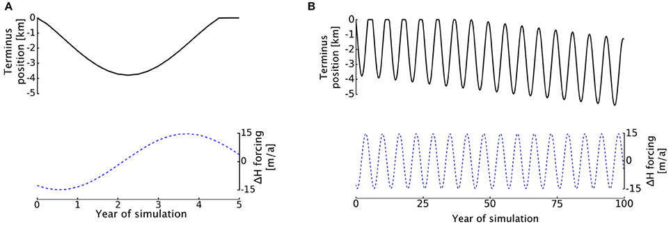
Figure 9. Pattern of retreat and readvance of Helheim Glacier simulated with a sinusoidal pattern of thinning-thickening upstream for 5 years (A) and 100 years (B). Black curves on the upper axes show the changing terminus position, and blue dotted curves below show the forcing over the course of the simulation.

Under the time-varying upstream forcing, our model shows Helheim's terminus undergoing multi-year cycles of retreat and readvance over a longer-term retreat signal. Data limitations preclude a direct comparison between our simulation and observed patterns of advance and retreat, but we note that the simulated retreat is of the correct order of magnitude. For 2 years, the terminus retreats at an average rate of 1.65 km a⁻¹ before slowing its retreat and readvancing, consistent with what was observed in the early 2000s (Howat et al., 2005; Murray et al., 2015). The 100-year simulation results also demonstrate that the model can capture short-term oscillations over a longer-term retreat, which is promising for eventual treatment of seasonal cycling.

3.4. Hubbard Glacier, Alaska—8 Auto-Selected Centerlines

Finally, we explore the performance of the plastic network method for a glacier with more complicated geometry. Hubbard Glacier is Alaska's largest tidewater glacier by area, covering 2450 km². Unlike many other tidewater glaciers in the region, and apparently independent of climate forcing, it thickened and advanced throughout the 20th century (Arendt et al., 2002; Trabant et al., 2003; Stearns et al., 2015). The advance has been well-documented due to the glacial outburst flood hazard created when the advancing glacier terminus closes Russell Fjord, which has happened twice in the past 30 years (Ritchie et al., 2008).

Huss and Hock (2015) have reconstructed ice thickness for Alaska glaciers following the method of Huss and Farinotti (2012). We estimate bed topography for Hubbard Glacier by subtracting that reconstructed ice thickness from a digital elevation model of the surface provided by Kienholz et al. (2015). The automated algorithm described by Kienholz et al. (2014) identifies 459 tributary centerlines on Hubbard Glacier, from which we choose the 8 that exceed 20 km in length. Figure 10 shows the bed topography underlying the network of eight branches, with automatically-selected centerlines of the branches in white and intersection points marked in red. Following the optimization procedure described above, we find the best model fit with τ_y = 200 kPa.

FIGURE 10

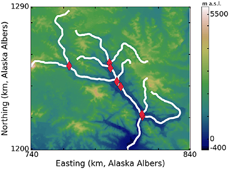
Figure 10. Eight branches of Hubbard Glacier (white) selected by Kienholz et al. (2014) with reconstructed bed topography from c.2007 (Huss and Farinotti, 2012; Huss and Hock, 2015). Red diamonds mark intersections of the branches.

Figure 11 shows the plastic model applied to all eight branches. Note that we have restricted the colorbar of Figure 11C to saturate at 100% error. Overall, model error on Hubbard Glacier is comparable to other cases, with mean error of +52% and median of +27%. The maximum underestimation of ice thickness is 52%, also comparable to other cases. However, the upper reaches of several branches show high error, with five points reaching 1000% error and an anomalously high 4237% overestimation of ice thickness found at one point in the main branch. The reconstruction method of Huss and Farinotti (2012) constrains ice thickness to be 0 at the ice divide, which likely accounts for such large increases in model error upstream (%_error = 100(H_model − H_recon)/H_recon). Indeed, the point with the highest percent error corresponds to a 747 m overestimation of ice thickness, which is only about 70% of the maximum observed ice thickness for Hubbard Glacier. We expect the plastic model to be more applicable close to the terminus—where stresses are higher and the ice is flowing faster—and the increasing error far upstream agrees with this expectation.

FIGURE 11

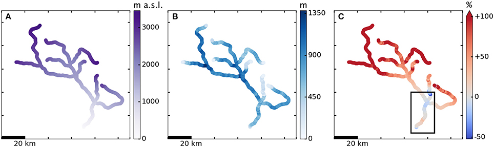
Figure 11. Plastic model with τ_y = 200 kPa applied to network of eight major tributaries of Hubbard Glacier, aerial view, c.2007. (A) Glacier surface elevation, (B) Ice thickness, (C) Percent error model-reconstruction (Huss and Farinotti, 2012; Huss and Hock, 2015). Black box on (C) indicates the region shown in Figure 12.

Observations of Hubbard Glacier are sparse above the lowest 15 km (Trabant et al., 2003) and the highest model error coincides with poorly-constrained areas of the glacier. Further, our optimization procedure shows that optimizing for τ_y over the lower 30 km of Hubbard Glacier provides the best, least sensitive fit to observation. For these reasons, we focus our attention on the better-constrained downstream portion of the glacier.

Figure 12 shows the plastic model results on the lower 30 km of Hubbard Glacier. The percent error of the model with respect to the reconstruction of Huss and Hock (2015) in this region is quite low, comparable to percent error on other glaciers. The maximum errors are 27.7% overestimation and 22.3% underestimation of ice thickness, a marked improvement on the error seen on the full eight-branch network.

FIGURE 12

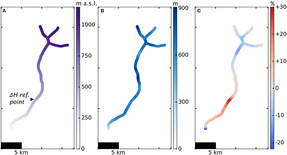
Figure 12. Plastic model with τ_y = 200 kPa applied to lower 30 km of network of Hubbard Glacier tributaries, aerial view, c.2007. (A) Glacier surface elevation, (B) Ice thickness, (C) Percent error model-reconstruction (Huss and Hock, 2015). Note that Figure 11 and this figure use different colorbars to best highlight the features of each.

3.4.1. Advance 1948-present

Previous case studies, as well as our earlier work on Columbia Glacier, documented that our plastic model reproduces observed patterns of retreat (Ultee and Bassis, 2016) as well as rudimentary multi-year cycles of advance and retreat. Now, using observations of the lowest 10 km of Hubbard Glacier from 1948 to the present, we investigate how well the model can reproduce observed tidewater glacier advance. Several published studies (Trabant et al., 2003; U. S. Geological Survey, 2003; McNabb and Hock, 2014) and a US Geological Survey dataset documenting the observed advance provide a useful basis for evaluation.

We choose a reference point 6 km upstream, where the successive longitudinal profiles of Trabant et al. (2003) show a total of 70 m of thickening between 1948 and 2000. The rate of thickening was not constant, but for simplicity we impose a constant rate equal to the 1948–2000 mean—approximately 1.3 m a⁻¹ at the reference point. We run the model for every year 1948-2000 with constant annual thickening, and find the terminus advance plotted in Figure 13. Mean terminus advance rate over the entire period is 29.7 m a⁻¹, and total advance 1948–2000 is 1.55 km. For comparison, black diamonds in Figure 13 show the advance reported by the USGS. The modeled total advance of 1.54 km 1948–2000 agrees with the total advance of 1.4 km reported by Trabant et al. (2003), as well as the 1.75 km advance reported for 1948–2012 by McNabb and Hock (2014). The mean advance rate of 29.7m a⁻¹ agrees with the 28m a⁻¹ rate reported by Trabant et al. (2003) and the 23−36m a⁻¹ reported by Stearns et al. (2015).

FIGURE 13

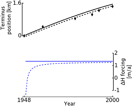
Figure 13. Simulated terminus advance of Hubbard Glacier, 1948–2000, under two different forcings. Black curves show plastic model advance under constant upstream thickening (solid) and under a fit to observed upstream thickening (dashed). Black diamonds give observed change in terminus position from USGS longitudinal profiles. Blue curves show the annual thickening rate imposed as an upstream forcing: constant (solid) and fit to observations (dashed).

Finally, we explore what can be gained by running the model with a more realistic forcing, deriving the upstream thickening from a fit to observations rather than the 52-year mean. We run the model with time-variable upstream thickening fit to observations and find the terminus advance shown by the dashed curve in Figure 13. The variable forcing produces more realistic advance, but only marginally so. Mean terminus advance rate over the entire period is 28.0 m a⁻¹, very similar to the mean advance rate found using a constant forcing. We conclude that using a constant average forcing is an acceptable simplification. For both forcings, our model shows advance rate decreasing over time, while observations show an increasing rate of advance punctuated by one slow period c.1972–1984 (Stearns et al., 2015). The construction of a moraine shoal through sediment buildup has been shown to be fundamentally important for tidewater glacier advance (Meier and Post, 1987; Oerlemans and Nick, 2006; Goff et al., 2012); we suspect that the lack of sediment transport in our plastic model prevents it from maintaining or accelerating rapid advance as a real glacier could.

4. Discussion

The yield strength τ_y, as the sole adjustable parameter of our model, merits careful examination. We note that there is not one single value of τ_y that works equally well for all observed glaciers; rather, there is variation in the best-fit values. The two Alaska glaciers studied are best fit by lower yield strengths (130–200 kPa), while the Greenland glaciers are best fit by higher yield strengths (245–355 kPa). We hypothesized that the greater physical sophistication of the Coulomb yield criterion would better match observed glacier profiles, but the results of our case studies are inconsistent on this point. For example, CV_RMS between modeled and observed main branch profiles is minimized with the Coulomb criterion for Columbia and Helheim Glaciers, but with the constant-yield-strength criterion for Jakobshavn Isbræ and Hubbard Glacier. We suggest that some of the diversity of yield-strength regimes found in our case studies is a reflection of glacier physics, and some is a side effect of the plastic model's simplicity. For example, the two Alaskan glaciers are temperate and receive much more precipitation than the Greenland outlet glaciers, which may contribute to the lower yield strengths of the former. If the model could be adjusted for ice-dynamical factors such as fjord width, temperature, presence of proglacial mélange or ice tongue, etc., we might expect to adjust for those factors with their own parameters and find a more consistent best-fit yield criterion across all observed glaciers. With τ_y as the only parameter of the model, however, it is reasonable that a diverse set of glaciers with unique characteristics would have similar diversity in their best-fit yield strengths. This phenomenon is also recognizable in the inter-branch yield strength disparity found for Helheim Glacier. Nevertheless, we note that the range of τ_y in our case studies is well within the range of laboratory and field observations (roughly 75–500 kPa).

For networks of two or more branches, we must also consider the inter-branch variability in best-fit τ_y. On Helheim Glacier, that variability is especially noteworthy, with more than 100 kPa difference in the best-fit Coulomb yield strength τ₀ between the small north-easternmost branch and the larger, deeper main branch. In the case studies presented here, we used a single value of τ_y (constant yield strength) or τ₀ (Coulomb yield condition) for all branches of a given glacier network, but future model development could include varying the yield strength by branch. To avoid discontinuities in surface slope, it would be necessary to vary the yield strength smoothly across the junction between branches rather than allowing a step change at the branch point.

Though our plastic network model fits observed profiles of tidewater glaciers remarkably well given its simplicity, some clear model weaknesses remain. For example, the simplest version of the model, making use of a single constant yield strength τ_y, cannot reproduce retreat that occurs while the glacier is thickening, nor advance that occurs while the glacier is thinning. In observed glaciers, upstream thinning usually corresponds to terminus retreat, and thickening to advance, but not always. For example, about 10% of the Alaska glaciers sampled by Arendt et al. (2002) exhibited thickening-retreat or thinning-advance. Further, the model response to forcing is instantaneous. Driving the model upstream produces instant change in terminus position, and driving the model at the terminus produces instant change in the upstream elevation profile. Therefore, we remain unable to comment on the causal relationship between retreat and thinning (see also Ultee and Bassis, 2016). More fundamentally, lack of a sediment transport mechanism hampers our model's simulation of realistic tidewater glacier advance, as illustrated by the Hubbard Glacier case study. Another obstacle to wide implementation of our model is the input data required: bed topography and bathymetry, which are not globally available. We have treated case studies of Columbia and Hubbard Glaciers, which are among the best-constrained Alaska tidewater glaciers. While extending the model to other Alaska tidewater glaciers seems a natural next step, further study is hampered by limited observational constraints on glacier bed topography.

4.1. Introducing Climate Forcing

The highly simplified model implementation presented here relies on manual input of an upstream thickening or thinning rate for each glacier. Manual input may be constrained by observational data, but it is a poor substitute for true climate forcing. Further, the technique is not scalable to the hundreds of tidewater glaciers worldwide, limiting the utility of the model. Two options exist to remedy this situation: introducing climate forcing directly into the plastic model, for example by adding functionality to treat changes in surface mass balance, or coupling upstream with a more sophisticated model that handles climate forcing itself. We discuss the first tactic in Bassis and Ultee (in review) and focus our attention here on the second tactic.

Coupling with a more complex glacier dynamics model (e.g., Marzeion et al., 2012) may be possible, but will require judicious choice of coupling location x_couple. We need only require that ice thickness remains continuous at the junction, but the best x_couple may depend on the glacier and the choice of upstream model. Without the benefit of coupling experiments to guide us, we suggest that the most consistent choice of x_couple will match not only ice thickness, but basal shear stress at the junction point. The plastic model assumes that basal stress over the entire glacier is exactly the yield strength of ice, τ_y, which may vary spatially according to the Coulomb condition of Equation (5) (see also Ultee and Bassis, 2016). In theory, basal stress of a tidewater glacier flowing down a valley without large pinning points should increase downstream throughout the accumulation area, which should be reflected in the glacier models with which our model could couple. The appropriate location to induce coupling, x_couple, is the point along the centerline of the main glacier branch where the basal stress according to the upstream model matches our model's yield strength of ice to within a certain tolerance. Large, abrupt features such as upstream ice falls—like the one on Columbia Glacier's main branch—may affect selection of x_couple. Careful initial experiments will help in designing a general method of avoiding such problems.

At x_couple, we require that the ice thickness of the plastic glacier, H_couple ≡ H(x_couple), match that found by the upstream model. As the upstream model evolves in time, the plastic glacier downstream will respond to changes in H_couple. In this way, the plastic model can respond to changes in climate forcing applied upstream. We note that the climate forcing relevant to tidewater glaciers includes not only atmosphere forcing, but ocean forcing as well. However, coupling our model to an ocean model at the calving front would be considerably more complicated to implement, and we have not explored that possibility.

5. Conclusion

We have presented a model that balances the simplicity of one-dimensional flowline modeling with the power of explicitly representing intersections between glacier branches. Our case studies indicate that the model can produce surface elevation profiles of multiple branches with low error, as well as realistically simulate the advance and retreat of Alaska and Greenland tidewater glaciers. Though our method gains important validation from detailed application to individual glaciers, its true appeal is in scaling up to large networks of tidewater glaciers, such as those draining the Greenland Ice Sheet. Simulation of those larger networks can be enhanced by explicit inclusion of surface mass balance—as described in Bassis and Ultee (2017, submitted manuscript)—or coupling to a more sophisticated model upstream.

Our initial case studies, performed without high-quality local climate data or coupling to a sophisticated ice dynamics model, give reason for optimism. In particular, the cases of Columbia Glacier (see Ultee and Bassis, 2016) and Hubbard Glacier demonstrate that a simple constant upstream forcing can reproduce terminus advance and retreat with surprising accuracy. More precise forcing based on observations of the glacier or the local climate does offer marginal improvement in model performance, as demonstrated for Hubbard Glacier above, but it is not essential. Thus, our model offers useful projections despite the inherent uncertainty in models of future climate.

Author Contributions

LU wrote the model, ran simulations, and wrote most of the manuscript. JNB provided direction in model development and collaborated in writing the manuscript. Both authors contributed to designing the project.

Funding

This work was supported by National Science Foundation grant ANT-114085 and the National Oceanic and Atmospheric Administration, Climate Process Team: Iceberg Calving grant NA13OAR4310096.

Conflict of Interest Statement

The authors declare that the research was conducted in the absence of any commercial or financial relationships that could be construed as a potential conflict of interest.

Acknowledgments

We thank Christian Kienholz, Matthias Huss, and Shad O'Neel for providing essential data.

References

Arendt, A. A., Echelmeyer, K. A., Harrison, W. D., Lingle, C. S., and Valentine, V. B. (2002). Rapid wastage of Alaska glaciers and their contribution to rising sea level. Science 297, 382–386. doi: 10.1126/science.1072497

PubMed Abstract | CrossRef Full Text | Google Scholar

Bassis, J. N., and Jacobs, S. (2013). Diverse calving patterns linked to glacier geometry. Nat. Geosci. 6, 833–836. doi: 10.1038/ngeo1887

CrossRef Full Text | Google Scholar

Bassis, J. N., and Walker, C. C. (2012). Upper and lower limits on the stability of calving glaciers from the yield strength envelope of ice. Proc. R. Soc. Lond. A Math. Phys. Eng. Sci. 468, 913–931. doi: 10.1098/rspa.2011.0422

CrossRef Full Text | Google Scholar

Church, J. A., Clark, P. U., Cazenave, J. M., Jevrejeva, S., Levermann, A., Merrifield, M. A., et al. (2013). “Sea level change,” in Climate Change 2013: The Physical Science Basis, eds T. F. Stocker, D. Qin, G. K. Plattner, M. Tignor, S. K. Allen, J. Boschung, A. Nauels, Y. Xia, V. Bex, and P. M. Midgley (Cambridge, UK; New York, NY: Cambridge University Press), 1137–1216.

Google Scholar

Cohen, D., Iverson, N. R., Hooyer, T. S., Fischer, U. H., Jackson, M., and Moore, P. L. (2005). Debris-bed friction of hard-bedded glaciers. J. Geophys. Res. Earth Surf. 110:F02007. doi: 10.1029/2004JF000228

CrossRef Full Text | Google Scholar

Cornford, S. L., Martin, D. F., Graves, D. T., Ranken, D. F., Brocq, A. M. L., Gladstone, R. M., et al. (2013). Adaptive mesh, finite volume modeling of marine ice sheets. J. Comput. Phys. 232, 529–549. doi: 10.1016/j.jcp.2012.08.037

CrossRef Full Text | Google Scholar

CReSIS (2016a). CReSIS L3 Radar Depth Sounder Data: Helheim Glacier. Available online at: http://data.cresis.ku.edu/

CReSIS (2016b). CReSIS L3 Radar Depth Sounder Data: Jakobshavn Isbræ. Available online at: http://data.cresis.ku.edu/

Csatho, B., Schenk, T., van der Veen, C., and Krabill, W. B. (2008). Intermittent thinning of Jakobshavn Isbræ, West Greenland, since the Little Ice Age. J. Glaciol. 54, 131–144. doi: 10.3189/002214308784409035

CrossRef Full Text | Google Scholar

Cuffey, K., and Paterson, W. (2010). The Physics of Glaciers, 4th Edn. Burlington; Kidlington: Elsevier Science.

Google Scholar

Enderlin, E. M., Hamilton, G. S., O'Neel, S., Bartholomaus, T. C., Morlighem, M., and Holt, J. W. (2016). An empirical approach for estimating stress-coupling lengths for marine-terminating glaciers. Front. Earth Sci. 4:104. doi: 10.3389/feart.2016.00104

CrossRef Full Text | Google Scholar

Goff, J. A., Lawson, D. E., Willems, B. A., Davis, M., and Gulick, S. P. S. (2012). Morainal bank progradation and sediment accumulation in disenchantment bay, alaska: response to advancing hubbard glacier. J. Geophys. Res. Earth Surf. 117:F02031. doi: 10.1029/2011JF002312

CrossRef Full Text | Google Scholar

Howat, I. M., Ahn, Y., Joughin, I., van den Broeke, M. R., Lenaerts, J. T. M., and Smith, B. (2011). Mass balance of Greenland's three largest outlet glaciers, 2000–2010. Geophys. Res. Lett. 38:L12501. doi: 10.1029/2011GL047565

CrossRef Full Text | Google Scholar

Howat, I. M., Box, J. E., Ahn, Y., Herrington, A., and McFadden, E. M. (2010). Seasonal variability in the dynamics of marine-terminating outlet glaciers in Greenland. J. Glaciol. 56, 601–613. doi: 10.3189/002214310793146232

CrossRef Full Text | Google Scholar

Howat, I. M., Joughin, I., Tulaczyk, S., and Gogineni, S. (2005). Rapid retreat and acceleration of Helheim Glacier, east Greenland. Geophys. Res. Lett. 32:L22502. doi: 10.1029/2005GL024737

CrossRef Full Text | Google Scholar

Huss, M., and Farinotti, D. (2012). Distributed ice thickness and volume of all glaciers around the globe. J. Geophys. Res. Earth Surf. 117:F04010. doi: 10.1029/2012JF002523

CrossRef Full Text | Google Scholar

Huss, M., and Hock, R. (2015). A new model for global glacier change and sea-level rise. Front. Earth Sci. 3:54. doi: 10.3389/feart.2015.00054

CrossRef Full Text | Google Scholar

Joughin, I., Abdalati, W., and Fahnestock, M. (2004). Large fluctuations in speed on Greenland's Jakobshavn Isbrae glacier. Nature 432, 608–610. doi: 10.1038/nature03130

PubMed Abstract | CrossRef Full Text | Google Scholar

Joughin, I., Smith, B. E., Howat, I. M., Floricioiu, D., Alley, R. B., Truffer, M., et al. (2012). Seasonal to decadal scale variations in the surface velocity of Jakobshavn Isbræ, Greenland: observation and model-based analysis. J. Geophys. Res. Earth Surf. 117:F02030. doi: 10.1029/2011JF002110

CrossRef Full Text

Joughin, I., Smith, B. E., Shean, D. E., and Floricioiu, D. (2014). Brief communication: further summer speedup of Jakobshavn Isbræ. Cryosphere 8, 209–214. doi: 10.5194/tc-8-209-2014

CrossRef Full Text | Google Scholar

Kienholz, C., Herreid, S., Rich, J. L., Arendt, A. A., Hock, R., and Burgess, E. W. (2015). Derivation and analysis of a complete modern-date glacier inventory for Alaska and northwest Canada. J. Glaciol. 61, 403–420. doi: 10.3189/2015JoG14J230

CrossRef Full Text | Google Scholar

Kienholz, C., Rich, J. L., Arendt, A. A., and Hock, R. (2014). A new method for deriving glacier centerlines applied to glaciers in Alaska and northwest Canada. Cryosphere 8, 503–519. doi: 10.5194/tc-8-503-2014

CrossRef Full Text | Google Scholar

Krimmel, R. M. (2001). Photogrammetric Data Set, 1957–2000, and Bathymetric Measurements for Columbia Glacier, Alaska. Reston, VA: US Geological Survey.

Google Scholar

Machguth, H., and Huss, M. (2014). The length of the world's glaciers—a new approach for the global calculation of center lines. Cryosphere 8, 1741–1755. doi: 10.5194/tc-8-1741-2014

CrossRef Full Text | Google Scholar

Marzeion, B., Jarosch, A. H., and Hofer, M. (2012). Past and future sea-level change from the surface mass balance of glaciers. Cryosphere 6, 1295–1322. doi: 10.5194/tc-6-1295-2012

CrossRef Full Text | Google Scholar

McNabb, R., Hock, R., O'Neel, S., Rasmussen, L., Ahn, Y., Braun, M., et al. (2012). Using surface velocities to calculate ice thickness and bed topography: a case study at Columbia Glacier, Alaska, USA. J. Glaciol. 58, 1151–1164. doi: 10.3189/2012JoG11J249

CrossRef Full Text | Google Scholar

McNabb, R. W., and Hock, R. (2014). Alaska tidewater glacier terminus positions, 1948–2012. J. Geophys. Res. Earth Surf. 119, 153–167. doi: 10.1002/2013JF002915

CrossRef Full Text | Google Scholar

Meier, M. F., and Post, A. (1987). Fast tidewater glaciers. J. Geophys. Res. Solid Earth 92, 9051–9058. doi: 10.1029/JB092iB09p09051

CrossRef Full Text | Google Scholar

Murray, T., Scharrer, K., James, T. D., Dye, S. R., Hanna, E., Booth, A. D., et al. (2010). Ocean regulation hypothesis for glacier dynamics in southeast greenland and implications for ice sheet mass changes. J. Geophys. Res. Earth Surf. 115:F03026. doi: 10.1029/2009JF001522

CrossRef Full Text | Google Scholar

Murray, T., Scharrer, K., Selmes, N., Booth, A. D., James, T. D., Bevan, S. L., et al. (2015). Extensive retreat of Greenland tidewater glaciers, 2000–2010. Arctic Antarctic Alpine Res. 47, 427–447. doi: 10.1657/AAAR0014-049

CrossRef Full Text | Google Scholar

Nye, J. F. (1951). The flow of glaciers and ice-sheets as a problem in plasticity. Proc. R. Soc. Lond. A Math. Phys. Eng. Sci. 207, 554–572. doi: 10.1098/rspa.1951.0140

CrossRef Full Text | Google Scholar

Nye, J. F. (1952). The mechanics of glacier flow. J. Glaciol. 2, 82–93. doi: 10.1017/S0022143000033967

CrossRef Full Text | Google Scholar

Nye, J. F. (1953). The flow law of ice from measurements in glacier tunnels, laboratory experiments and the Jungfraufirn borehole experiment. Proc. R. Soc. Lond. A Math. Phys. Eng. Sci. 219, 477–489. doi: 10.1098/rspa.1953.0161

CrossRef Full Text | Google Scholar

Oerlemans, J., and Nick, F. (2006). Modelling the advance–retreat cycle of a tidewater glacier with simple sediment dynamics. Glob. Planet. Change 50, 148–160. doi: 10.1016/j.gloplacha.2005.12.002

CrossRef Full Text | Google Scholar

O'Neel, S., Pfeffer, W. T., Krimmel, R., and Meier, M. (2005). Evolving force balance at Columbia Glacier, Alaska, during its rapid retreat. J. Geophys. Res. Earth Surf. 110:F03012. doi: 10.1029/2005JF000292

CrossRef Full Text | Google Scholar

Rignot, E., Mouginot, J., Larsen, C. F., Gim, Y., and Kirchner, D. (2013). Low-frequency radar sounding of temperate ice masses in southern Alaska. Geophys. Res. Lett. 40, 5399–5405. doi: 10.1002/2013GL057452

CrossRef Full Text | Google Scholar

Rignot, E., Velicogna, I., van den Broeke, M. R., Monaghan, A., and Lenaerts, J. T. M. (2011). Acceleration of the contribution of the greenland and antarctic ice sheets to sea level rise. Geophys. Res. Lett. 38:L05503. doi: 10.1029/2011GL046583

CrossRef Full Text | Google Scholar

Ritchie, J. B., Lingle, C. S., Motyka, R. J., and Truffer, M. (2008). Seasonal fluctuations in the advance of a tidewater glacier and potential causes: Hubbard Glacier, Alaska, USA. J. Glaciol. 54, 401–411. doi: 10.3189/002214308785836977

CrossRef Full Text | Google Scholar

Stearns, L. A., and Hamilton, G. S. (2007). Rapid volume loss from two East Greenland outlet glaciers quantified using repeat stereo satellite imagery. Geophys. Res. Lett. 34:L05503. doi: 10.1029/2006GL028982

CrossRef Full Text | Google Scholar

Stearns, L. A., Hamilton, G. S., vander Veen, C. J., Finnegan, D. C., O'Neel, S., Scheick, J. B., et al. (2015). Glaciological and marine geological controls on terminus dynamics of Hubbard Glacier, southeast Alaska. J. Geophys. Res. Earth Surf. 120, 1065–1081. doi: 10.1002/2014JF003341

CrossRef Full Text | Google Scholar

Straneo, F., Heimbach, P., Sergienko, O., Hamilton, G., Catania, G., Griffies, S., et al. (2013). Challenges to understanding the dynamic response of Greenland's marine terminating glaciers to oceanic and atmospheric forcing. Bull. Amer. Meteorol. Soc. 94, 1131–1144. doi: 10.1175/BAMS-D-12-00100.1

CrossRef Full Text | Google Scholar

Trabant, D. C., Krimmel, R. M., Echelmeyer, K. A., Zirnheld, S. L., and Elsberg, D. H. (2003). The slow advance of a calving glacier: Hubbard Glacier, Alaska, U.S.A. Ann. Glaciol. 36, 45–50. doi: 10.3189/172756403781816400

CrossRef Full Text | Google Scholar

Ultee, L., and Bassis, J. N. (2016). The future is Nye: an extension of the perfect plastic approximation to tidewater glaciers. J. Glaciol. 62, 1143–1152. doi: 10.1017/jog.2016.108

CrossRef Full Text | Google Scholar

U. S. Geological Survey (2003). Hubbard Glacier, Alaska: Growing and Advancing in Spite of Global Climate Change and the 1986 and 2002 Russell Lake Outburst Floods. USGS Fact Sheet 001-03.

van den Broeke, M. R., Enderlin, E. M., Howat, I. M., Kuipers Munneke, P., Noël, B. P. Y., van de Berg, W. J., et al. (2016). On the recent contribution of the greenland ice sheet to sea level change. Cryosphere 10, 1933–1946. doi: 10.5194/tc-10-1933-2016

CrossRef Full Text | Google Scholar

Vaughan, D. G., Comiso, J., Allison, I., Carrasco, J., Kaser, G., Kwok, R., et al. (2013). “Observations: cryosphere,” in Climate Change 2013: The Physical Science Basis, eds T. F. Stocker, D. Qin, G. K. Plattner, M. Tignor, S. K. Allen, J. Boschung, A. Nauels, Y. Xia, V. Bex, and P. M. Midgley (Cambridge, UK; New York, NY: Cambridge University Press), 317–382.

Google Scholar