Inference of Soil Hydrologic Parameters from Electronic Soil Moisture Records

Introduction

Soil moisture is an important control on hydrologic function, as it governs vertical fluxes from and to the atmosphere, groundwater recharge, and lateral fluxes through the soil (Loik et al., 2004; Grayson et al., 2006; Vereecken et al., 2008). Soil moisture is also an excellent metric of hydrologic model performance, as it integrates temporal variation in precipitation and evaporation and is responsive to topography and soil physical properties governing fluxes of water (Wood et al., 1992; Cuenca et al., 1996; Rodriguez-Iturbe et al., 1999, 2001; Laio et al., 2001; Western et al., 2004; Seneviratne et al., 2010; Bandara et al., 2013; Or et al., 2015; Paniconi and Putti, 2015). As such, the definition and quantification of physical properties that govern the ability of a soil to retain water against gravity drainage, evaporation, and transpiration have long been of interest to agronomists and physical scientists (Briggs and McLane, 1907; Buckingham, 1907). However, measurement of relevant soil physical properties has historically been conducted in laboratories, which may not represent the behavior of water in field conditions. Techniques to measure soil moisture in the field have improved dramatically in recent decades so that near-continuous measurements are now routine. In this paper we demonstrate how multiple years of near-continuous measurements of soil water content can improve estimates of hydrologically relevant soil properties.

The physical properties of soils determine several important thresholds in Θ, defined as the volumetric fraction of water in a unit volume of soil (m³ m⁻³): Soil saturation is conventionally defined as the condition when the entire pore volume is filled with water (Θ_s), which typically occurs only during subirrigation. The Θ at which gravity drainage effectively ceases has been termed field capacity (FC; Veihmeyer and Hendrickson, 1949), and the Θ at which transpiration ceases has been termed permanent wilting point (PWP; Briggs and Shantz, 1912). The difference in the value of FC and PWP is often used to estimate plant available water (Hansen et al., 1980) and the difference in the value of Θ_s and PWP is similarly used to estimate root zone storage (Seneviratne et al., 2010). Unfortunately, most measurements of these important field-scale properties are performed in laboratories on small samples.

The prevailing concepts of FC and PWP are a legacy of efforts to relate soil hydraulic and hydrologic parameters to standardized measurements of soil physical properties. Briggs and McLane (1907), introduced a “moisture equivalent” as a water to soil mass fraction for samples that were air dried, screened through a 2 mm sieve, packed in cylinders, saturated, and spun to achieve a force 1,000 times the force of gravity. These results were later expanded to analysis of PWP of wheat seedlings in a controlled study over a range of soil textures (Briggs and Shantz, 1912). Meinzer (1923) later defined “specific retention” as the volumetric fraction of water retained after long term drainage from saturation, which has been determined by measurement in small cells of disturbed soils (Hazen, 1892), and in situ (Ellis and Lee, 1919). Piper (1933) aptly concluded that experimental scale and depth of the capillary fringe exerted important controls on the results. Subsequently, Richards and Weaver (1944) built on the work of Buckingham (1907) to systematize measurement of matric potential (Ψ)-Θ relationships. Using the pressure plate technique, they equated the Θ at −33 kPa to the “moisture equivalent” for 71 near surface samples of irrigated soils (Richards and Weaver, 1944). The use of −10 kPa to determine Θ at field capacity was reserved for coarse and volcanic soils. These advancements led to the development of capillary permeability relations for isotropic porous media (Burdine and Redford, 1952; Brooks and Corey, 1964) and continuous Ψ-Θ conductivity models (Mualem, 1976) that remain in use.

The validity of these historic terms as physical constants has been widely criticized (Miller and McMurdie, 1953) resulting in refinements and additional terms for use in fields beyond agronomy. For example, it is understood that saturation may never be achieved in well drained soils under field conditions (Wang et al., 1998). Field saturation, Θ_fs, accounts for gas filled soil pore space that may be occluded within the pore matrix at approximately the bubbling pressure (Reynolds et al., 2002) and can occur due to air encapsulation (Fayer and Hillel, 1986), fluctuating groundwater levels (Marinas et al., 2013), and biogenic gases (Morse et al., 2015).

Field capacity has been criticized because the end point for gravity drainage is unclear and possibly method dependent due to differences in boundary conditions and scale (Colman, 1947; Hillel, 1980; Cassel and Nielsen, 1986; Kirkham, 2005). As a result, Ψ-values from −33 to −5 kPa have been proposed to define FC (Richards and Weaver, 1944; Salter and Haworth, 1961; Linsley and Franzini, 1972; Romano and Santini, 2002; Kirkham, 2005; Nemes et al., 2011). More recently, Assouline and Or (2014) proposed a method to relate the slope of the soil characteristic curve (n), the air entry value (Ψ_ae) and the residual water of a soil (Θ_r) (van Genuchten, 1980) to a soil specific FC, based on the balance between capillary and gravitational forces. This dynamical approach seeks to transcend the use of static arbitrary values.

PWP has been criticized because the actual wilting point is species and soil texture dependent and, in the case of many native plants adapted to dry conditions, transpiration can cease with no wilting at Ψ in the range of −3 to −5 MPa for both tree and grass species (Scholes and Walker, 1993; Damesin and Rambal, 1995; Sperry et al., 2002; Rambal et al., 2003). To address these issues, Seyfried et al. (2009) used the term “plant extraction limit” (PEL) in place of PWP to describe the Θ below which plants cannot extract water, and evaporation is the primary means of soil water loss. Therefore, Θ at PEL is likely to be equal to or greater than Θ at the limit of capillary continuity (Lehmann et al., 2008; Assouline and Or, 2014), since evaporation can continue following the cessation of plant water use.

Furthermore, between FC and PEL, there is range of declining Ψ over which plant stress increases and evapotranspiration decreases (Rodriguez-Iturbe et al., 1999). This range of Ψ and the related range of Θ is associated with a shift from energy-limited to soil moisture potential-limited evapotranspiration (Budyko, 1956; Koster et al., 2009). The threshold in water content between these states in terms of Θ has been defined as s* (Laio et al., 2001; Rodriguez-Iturbe et al., 2001), Θ_crit (Koster et al., 2004; Seneviratne et al., 2010), or Θ_ws (Smith et al., 2011) and conceptualized as an inflection point in evaporation-soil water content relation models. Similarly, Buckingham (1907) proposed that evaporation from soil is initially limited by moisture content, and secondly by vapor diffusion. Various formulations (Idso et al., 1974; Brutsaert and Chen, 1995) and methods have since been used to determine energy limited (Stage I) and supply/transport limited (Stage II) evaporation from soils (Salvucci, 1997). Stage III is vapor diffusion transport (Metzger and Tsotsas, 2005; Lehmann et al., 2008). During the second and third stages, the vaporization plane (e.g., drying front) will move downward from the soil surface as evaporation proceeds (Shokri et al., 2008; Shokri and Or, 2011). Therefore, the annual endpoint of soil drying may range from a value less than FC, to near the hygroscopic point, depending on the characteristics of local climate, soil, and plants (Laio et al., 2001).

The current capacity to resolve soil hydrologic properties and Θ at scales sufficient to parameterize and validate distributed hydrologic models remains challenged by the relatively limited data available to define spatial heterogeneity and effective scales of measurement (Njoku et al., 2003; Reichle et al., 2007; Huang et al., 2016). Since transitions in fluxes in agronomic and ecohydrologic models are often indicated by FC, Θ_ws, and PEL either indirectly (Liang et al., 1996) or directly (e.g., Wigmosta et al., 1994; Boote et al., 2008; Seneviratne et al., 2010; Paniconi and Putti, 2015) and are bounded by Θ_s (or Θ_fs) and either PEL or some lower limit to Θ, we consider these important variables for hydrologic modeling. Recent approaches to determine soil moisture parameters include inverse modeling, remote sensing and other synthetic approaches (Santanello et al., 2007; Montzka et al., 2011; Bandara et al., 2013). However, soil hydrologic properties would ideally be determined by field measurement (Romano and Santini, 2002). Hillel (1980) recommended that properties such as FC must be measured repeatedly in the field, after the entire depth of the soil profile is wetted and that laboratory methods based on Ψ equivalent to −1.5 MPa, −33 kPa, or −10 kPa matric potential are arbitrary static measurements that are not representative of systems with external controls on the soil boundary conditions, such as poor drainage or evaporation.

Given the increasing availability of electronic measurements of soil water content and considerable theoretical and conceptual controversy regarding soil water content constants, the primary objective of this paper is to determine if temporal patterns of measured soil water content values are consistent with the concepts of Θ_s, FC, and PEL. The proposed methods presented here are intended to determine consistent and physically/ecologically relevant estimates of these soil hydrologic parameters directly from long term field measurements of Θ. We pose the hypothesis: Data attractor values and inflections in Θ time series records represent changes in dQ/dt that are consistent with the concepts of FC, Θ_ws, and PEL. This is based on prior observations that FC and PEL exist as quasi-stable states (Miller and Klute, 1967; Cassel and Nielsen, 1986; Kirkham, 2005) following periods of drainage and evaporation. These states are represented by greater data frequency (data attractors) at intermediate and low values of Θ. That is, following input events, Θ rapidly trends toward FC where it is relatively stable due to capillary forces until decreases by evapotranspiration or increased by input flux greater than the associated unsaturated hydraulic conductivity [K(Θ)]. Then, as soils dry they stabilize near PEL. Thus, FC may be better represented in the absence of strong ET, such as during winter in mid-latitude regions, and PEL is best determined when energy does not limit transpiration. To test the hypothesis, we first compare soil hydrologic property values determined by four methods of analysis to and then assess the accuracy of the estimated values to values determined from a range physical methods at traditional soil water potentials. Finally, we evaluate the applicability of the tested approaches to other environments.

Setting

The analysis exploits the wide range and regular seasonal changes in soil moisture at sites near Boise ID, USA. In semiarid Mediterranean climates, seasonal patterns in soil moisture storage and streamflow follow seasonal changes in precipitation, temperature, and solar radiation (McNamara et al., 2005: Flerchinger et al., 2010; Seyfried et al., 2011). In this system, the water year begins with dry soil following the annual summer drought. As autumn rains arrive, the soil wets downward from the soil surface and soil profile water storage increases over a long wet period due to winter rains or snow melt. In spring, warming temperatures drive snowmelt and the annual hydrograph. Ultimately, precipitation decreases and plant water use depletes soil moisture as summer proceeds. In many years, this hydrologic setting imposes different soil surface boundary conditions in each season; intermittent surface wetting of the dry soil in fall, low flux snow melt in winter, high flux snow melt in spring and progressive soil drying over the summer (Figure 1).

FIGURE 1

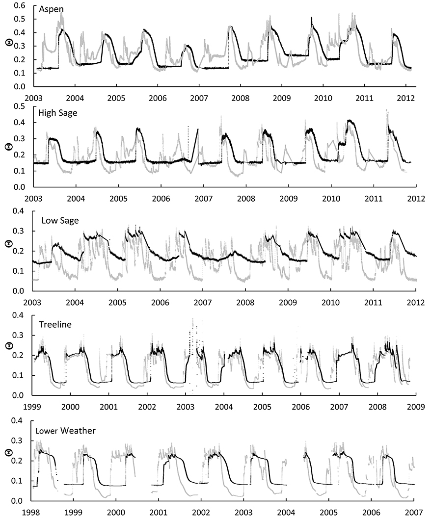
Figure 1. Annual time series in Θ for sensors near the soil surface (gray), and at the lowest measurement location (black), for the period of record. Data records are shown for Aspen (10, 180 cm), High Sage (10, 120 cm), Low Sage/W (10, 50 cm) Treeline and Lower Weather (15, 100 cm). Data are displayed by water year with Oct. 1 as the first day of the water year.

Sites

Data were collected from five sites at two watersheds in southwest Idaho, Reynolds Creek Experimental Watershed (RCEW) and Critical Zone Observatory operated by the USDA Northwest Watershed Research Center and Dry Creek Experimental Watershed (DCEW) operated by Boise State University. Data for RCEW are available at http://www.ars.usda.gov/Research/docs.htm?docid=8281 and from Seyfried et al. (2001) and Chauvin et al. (2011). Data for DCEW are available at http://earth.boisestate.edu/drycreek/.

The Upper Sheep Creek watershed is located within the Reynolds Creek Experimental Watershed, in the Owyhee Mountains of southwestern Idaho. The site ranges in elevation from 1,840 to 2,036 mamsl and is underlain by basalt bedrock. Mean annual precipitation is 426 mm, about 60% of which is snow. The snow is redistributed by wind, resulting in snow accumulations of 3–4 m in drifts and <15 cm in scour zones. Deposition patterns are persistent and result in distinctive snow-soil-vegetation complexes (Flerchinger et al., 1998; Prasad et al., 2001; Chauvin et al., 2011). The low sagebrush complex (Low Sage) is found on shallow (<50 cm deep) soils on mostly west-facing slopes and ridges. Soil textures are loam in the upper 10–20 cm and clay loam and gravel in the subsoil below the argillic horizon. The mountain sagebrush complex (High Sage) is on deeper soils, about 1 m thick, and mostly on north-facing slopes. The aspen complex (Aspen) is on deep (>2 m) soils and are closely associated with snow drifts. Soils in the High Sage and Aspen complexes were formed in aeolian deposits and are highly uniform with depth, mostly categorized as silt loam. Upper Sheep Creek was burned by a prescribed fire in summer 2007. The Big Sage area burned completely, and was replaced with grasses and forbs by 2008. The Aspen was cut down and recovered, in a hydrologic sense, by 2009.

The Treeline and Lower Weather sites are located in the Dry Creek Experimental Watershed (DCEW) in the foothills of the Rocky Mountains of southwestern Idaho. The elevation of these sites is 1,620 mamsl at Treeline and 1,150 mamsl at Lower Weather. Both sites are underlain by weathered granite from the Idaho Batholith, although the Lower Weather site is below the shoreline of prehistoric Lake Idaho. Mean annual precipitation is 520 mm at Treeline and 300 mm at Lower Weather. Over the period of measurement, snow accounted for ~50% of precipitation at Treeline (Kormos et al., 2014) but Lower Weather receives mostly rain. Similar to Upper Sheep Creek, geologic processes including wind scour have formed deeper soils on north facing slopes at Treeline and snow accumulation up to 2 m currently enhances springtime soil water where the sensors for this study are located. The vegetation at the site is typical of a transition between lower elevation grass-lands and higher elevation forests; mountain big sagebrush and ceanothus shrubs, prunus subspecies, forbs, and grasses. The Lower Weather site is not subject to drifting due to the limited snowfall at the lower elevation. Soil texture at DCEW is sandy loam and ranges in depth up to 1.3 m (Gribb et al., 2009; Tesfa et al., 2009).

Methods

Data Collection and Conditioning

Soil water content data were collected from representative sites of each of the five soil/vegetation complexes. These sites represent various controls of soil texture, soil depth, vegetation, and annual precipitation (Flerchinger et al., 2010) on Θ (Figure 1). In each instance, a pit was hand-excavated to bedrock or saprolite and two parallel profiles of soil moisture instruments, separated by 2 m, were installed horizontally into the pit face. A summary of sensor depths, soil texture and mean annual precipitation or estimated annual soil water input is provided in Table 1. At Upper Sheep Creek, hourly data were collected with time domain reflectometers (TDR 100, Campbell Sci., Logan UT, USA), with 3-prong, 30 cm long rods. Data are reported on water year basis. At Dry Creek, hourly data were collected with frequency domain reflectometers (CS615, Campbell Sci., Logan UT, USA) calibrated with less frequent samples from co-located TDR waveguides (Chandler et al., 2004). Data were prepared for analysis by removing most electronic noise, out of range data or data from failed sensors (Nayak et al., 2008; Kormos et al., 2014) and are reported by calendar year. Data cleaning did not include removal of records during periods of frozen soil, which were most prominent within 15 cm of the soil surface and affected a limited number of sensors. Frequency distribution of Θ from single sensors was done by constructing histograms from the conditioned data. The frequency analysis of temporally coincident data from paired sensors was done by binning data in two dimensional frequency arrays with increments of 0.01 Θ for 0.0 < Θ < 0.65.

TABLE 1

Table 1. Sensor location, mean annual soil water input (SWI), and soil texture.

Limited laboratory and field analyses are used to relate the results of the developed methods to traditional capillary pressure-saturation techniques. Measurements from a 66 kPa field tensiometer co-located with the 60 cm TDR sensor at Aspen site represent the range from field-saturated conditions just after snowmelt on May 20, 2004 to the time of removal on August 8, 2004. Laboratory measurements of Ψ over the ranges of 1.4–430 kPa (HYPROP, UMS GMBH, Munich Germany), and Ψ and Θ (corrected for bulk density) 0.2–115 MPa (dewpoint psychometer, Decagon Devices, Pullman WA, USA) and Θ were made to construct characteristic curves for soil samples collected at depths of 0–3 and 41–43 cm. At Treeline, soil water potential was previously measured in a field experiment to determine FC by surface irrigation from dry initial conditions. The experiment was interrupted by rain during the drainage period and terminated when the tensiometer lost capillary connection to the soil at ~33 kPa. Soil water potential was monitored by automated tensiometers (Gribb et al., 2009).

Values of Θ measured during the natural cycle of wetting and drying provide the basic data used in this analysis. In all cases the soils are well drained, therefore there is no attractor at or near soil saturation. We define attractors as values of Θ that occur at high frequency and develop four analyses that are based on observations made in a climate with distinct annual wet and dry phases. Field Saturation is the maximum observed value of Θ. Since complete soil saturation is infrequent in well drained field soils, the maximum annual value of Θ_fs is likely to range between FC and Θ_s. Field Capacity is a moisture state that prevails under wet, low flux conditions. In well-drained conditions, saturated soils drain quickly to near FC, then more slowly. Where soil water potential (Ψ) is seasonally affected by plant water uptake, FC may vary slightly with diel changes in evapotranspiration. Conversely, dry soils wet to a Θ somewhat greater than FC before drainage begins. These two processes enhance the local data frequency near FC and result in a data attractor that we define as the “wet attractor.” Figure 2A shows a wet attractor near Θ of 0.20 throughout the winter months when drainage is minimal and transpiration is insignificant. We propose that this attractor is approximately equivalent to FC. Several other descriptive and mechanistic definitions of FC have been developed and are presented by Assouline and Or (2014), who suggest the stability of soil water retention is a function of disruption of liquid phase continuity. Plant Extraction Limit is the Θ at which existing vegetation does not extract soil water by transpiration. Conceptually similar to the PWP, PEL allows for variations among soil-plant combinations and acknowledges that the vegetation doesn't necessarily wilt when transpiration ceases (or becomes very slow). PEL is expected to be an attractor in environments with extended dry periods and perennial vegetation. Under these conditions, Θ declines during the dry season until PEL is reached, then remains unchanged until replenished with new rainfall or snowmelt except near the soil surface, which may be subject to direct evaporation and may proceed to values less than the PEL. These processes result in a “dry attractor” in the data. Plant Water Stress Initiation (Θ_ws) is not an attractor, but is a decrease in plant water use as governed by complex physiological traits that control stomatal aperture (Osakabe et al., 2014), and is an inflection in soil moisture records (Rodriguez-Iturbe et al., 1999; Smith et al., 2011) determined as d²Q/dt2 > 0.

FIGURE 2

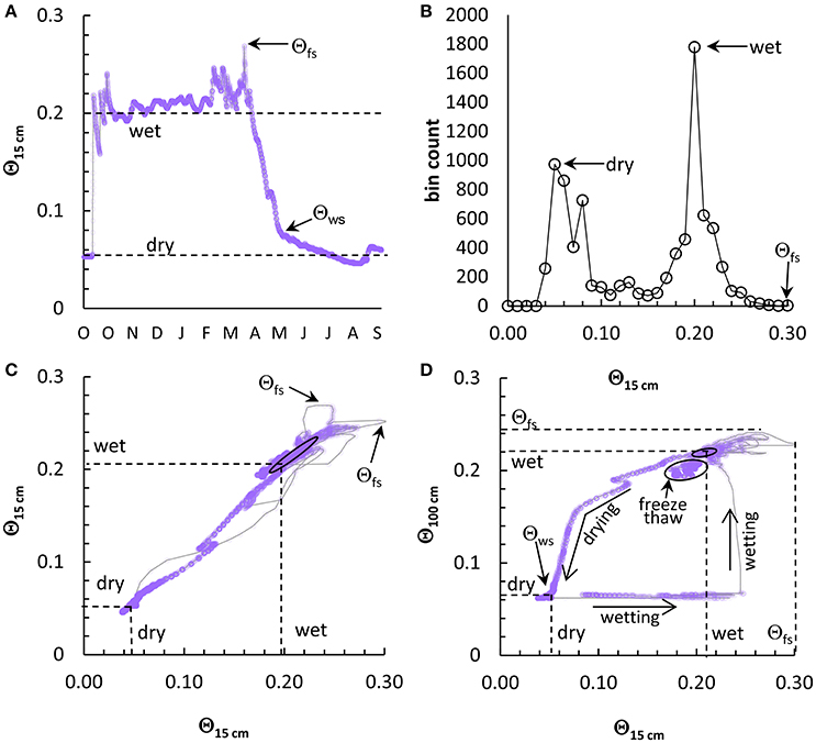
Figure 2. Four proposed methods to determine field saturation (Θ_fs), field capacity (FC) plant stress initiation (Θ_ws), and plant extraction limit (PEL) from Θ data measured at Treeline in 2001: (A) annual time series of Θ at 15 cm depth with visual estimates of FC and PEL. (B) Frequency analysis of Θ at 15 cm with high modes indicating wet and dry attractors and the annual maximum Θ as Θ_fs. (C) Paired measurements at 15 cm with FC and PEL data attractors identified by maximum paired frequencies and Θ_fs identified as the maximum value for each sensor. (D) Hysteresis of Θ at 15 and 100 cm depths with wet and dry state data attractors and Θ_fs identified for both soil depths. The counterclockwise VWC hysteresis trace shows distinct periods of surface wetting and soil profile wetting for 15 and 100 cm sensors and two inflections in the drying limb. Θ_crit at 10 cm depth is determined as the initiation of declining dQ/dt. Panels (A,C,D) display 15-min data as semitransparent markers to display data attractors by superposition. “Wet” data attractors are identified by ovals in (C,D).

Analysis Methods

Four methods of analysis to determine the parameters PEL, FC, and Θ_fs are presented. Throughout the remainder of the paper, these analyses will be referred to as time series, frequency, paired, and hysteresis, respectively.

Visual inspection of Θ records in time series is a simple approach to identify approximate values for each parameter for individual soil depths. Figure 2A shows this approach for one year of data from a 15 cm sensor at Treeline. At this site the minimal overlap between periods of slow drainage in winter and consistently low Θ in spring and summer. This allows subjective approximation of the wet and dry attractors, and clearly shows the maximum annual Θ, and an inflection in Θ(t) indicating a reduction in plant water use.

Frequency analysis of Θ distributions for single sensors show modal peaks in Θ at dry and wet soil moisture attractors for water year (Figure 2B) or period of record data. The maximum value of Θ is assumed to be equivalent to Θ_fs.

Paired sensors at similar depth, are often used to determine an average value of Θ, increase spatial representation of the measurement, or provide redundant data in case of instrument failure. These synchronous data can be plotted as x-y coordinates to determine high frequency attractors and extreme values. Figure 2C shows example data for a water year from paired sensors at 15 cm depth in soil pits separated by 2 m. Ideally, data pairs of Θ from paired sensors at similar depth will fall on a 1:1 line, bounded by the minimum and maximum Θ at the sensor depth. However, differences in the timing of wetting and drying result in divergence and spreading around a 1:1 line. In the example for one water year of data, Θ attractors emerge at dry Θ (≈0.05) and wet Θ (0.19–0.24) attractor values, respectively and the greatest measured values of Θ (0.30, 0.27) for Θ_fs on the respective axes of each sensor. Although, similar to the frequency analysis, the paired sensor analysis leverages twice as many sample locations per data point. The use of data pairs decreases the influence of erroneous or extreme values on the frequency of values near the data attractors on the central trend. Additionally, the resulting variance around the trend may provide the user greater guidance on the range of local variability in soil hydrologic properties than would a single sample location.

Hysteresis is often observed in the temporal behavior of Θ over seasonal wetting and drying periods for sensors at two depths in a vertical profile. The lag in both wetting and drying periods between the two depths enhances the relative frequency of wet and dry attractors, near the intersection of the wetting and drying limbs of the hysteresis loop. For example, Figure 2D shows hysteresis between Θ at 15 and 100 cm at Treeline. For the climate of this study, the water year begins near the end of the dry season, with Θ at near minimum values for both the surface and bottom of the soil profile. Accordingly, the Θ trace for a water year begins near the low Θ attractor. As autumn precipitation increases Θ at 15 cm depth, the Θ at 100 cm depth remains nearly constant until the wetting front arrives. For a water year at the example site, the horizontal wetting trace provides strong visual support for the interpretation of low Θ attractor from the small range in the ordinate. Along the right side of Figure 2D, wetting at the deep sensor is shown as the vertical trace up to the wet attractor, found at the intersection of the wetting and drying traces and identified by the black oval. As above, the maximum values on either axis represent Θ_fs. Finally, the drying limb terminates at the dry Θ attractor and provides visual support for identification of the dry Θ attractor for depth of the shallow sensor.

Results

We found wet and dry attractors within the expected ranges of FC and PEL by each of the presented methods, equated Θ_fs to the maximum value of Θ and interpreted the inflection during the drying phase, d²Q/dt2 as Θ_ws. Results from the time series, frequency, paired sensors, and hysteresis approaches are in general agreement, although each has a different bias. Below, we first present detailed graphical results from the paired and hysteresis analyses to demonstrate the attractors for the Aspen, Treeline, and Low Sage sites, which span the range of soil texture and climate among the study sites. Then we compare values determined by these methods at three depths for each site with results from the time series and frequency analyses. Example data from soil physics experiments performed in the laboratory and from in situ measurements at Aspen and Treeline sites are then provided to relate the extreme values and data attractors to PEL, FC, and Θ_fs.

Paired Sensors

Figure 3 shows two visualizations of paired sensor analyses over the study period for Aspen (90 cm), Low Sage (10 cm), and Treeline (15 cm). Here, and below, we present data that demonstrate analyses over the broadest range in soil texture, soil depth, and vegetation class. For the Aspen the top panel shows semi-transparent data points with makers to represent the data attractors and the bottom panel shows color maps of log-transformed data frequency values. Many of the paired sensors at a depth, such as Aspen, 90 cm show a strong linear correlation between sensors (central trend) with occasional hysteresis traces outside of the central trend. Shallow paired sensors such as at Low Sage and Treeline (Figure 3) show much greater variability in Θ around the central trend. These features result from the temporally local hysteresis between sensors during input events, repeated over the annual period of changes in Θ.

FIGURE 3

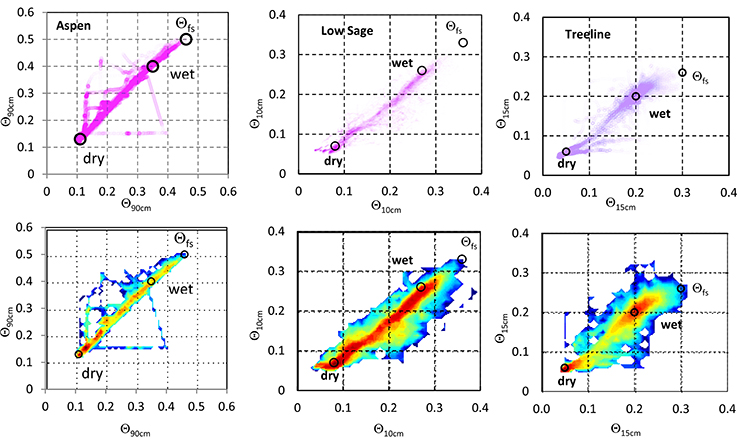
Figure 3. Example plots of Θ data from paired sensors at 90 cm at the Aspen site 10 cm at Low Sage site and 15 cm at the Treeline site over a 10-year record. In the top panel, data markers are 99% transparent to highlight high frequency areas by superposition. Circular data markers are placed at points of maximum frequency corresponding to dry and wet attractors, and maximum values at Θ_fs. The bottom panel shows the same data as the upper panel as color maps of log transformed frequency data for each 0.01 by 0.01 cell of Θ data with an arbitrary scale from low (blue) to high (dark red) frequency.

Comparison of plots of raw data in the upper panel of Figure 3 with the log transformed frequency colormaps in the lower panel demonstrates the greater visual support of the transformed data for identification of attractor values. Whereas, the point values can be selected directly from the frequency value matrix, as was done to identify attractors for the upper panel, the colormaps simplify the interpretation of the frequency value matrix. In Figure 3 (lower panel) dry attractors for the period of record are clearly shown as dark red points in the colormaps, often near the minimum Θ, and are generally surrounded by a set of high frequency values which may include two or three modes. Similarly, the period of record wet attractor value is often diffuse, with weak frequency modes for the Aspen (silt loam) and Low Sage (clay loam) sites, but with a more distinct attractor for the Treeline (sandy) site. Variability between sensors extends to Θ_fs, which varies more by depth and year than the other paired analyses because it is an extreme value. The minimum and maximum of annual estimates (Table 2) bound the period of record estimates, and provide an approximation of the range in variability of the determined values. For the Treeline site, the range in annual estimates for individual sensors within the paired sensor configuration was zero to 0.02 Θ for both the attractors and Θ_fs, likely due to the high sand content at this site. At Low Sage and Aspen, the range increased progressively to 0.01–0.05 Θ and 0–0.11 Θ, respectively, primarily due to annual variability in Θ at depth. Spatial differences in Θ(t) resulted in variance from unity slope (1.00) for many sites and depths, but were similar within soil texture class: For the Aspen and High Sage sites the slope of the relation between paired sensors increased from a slope of 1.00–1.03 near the soil surface to as much as 1.33 at depth. At Low sage the slope of the relationship ranged from 1.10 to 1.19 from 10 to 40 cm depth, and 1.36 at 50 cm, in the C horizon, which is very stony. The Treeline and Lower Weather sites have low bulk density surface soil, with frequent macropores the slope of the trend at 5 cm depth (1.17–1.29) is much greater than for the deeper, stony soils (1.12).

TABLE 2

Table 2. Period of study maximum and minimum annual values of wet and dry data attractors (Θ) and Θ_fs for sensor pairs at a range of depths (cm) at selected sites.

Hysteresis plots of Θ for period of study data at Aspen, Low Sage, and Treeline show more complex wet and dry data attractors than are shown for an annual cycle in Figure 2D. Figure 4 presents visualizations of hysteresis between shallow and mid-profile depths, mid-profile and deep sensors, and log transformed colormaps of selected plots.

FIGURE 4

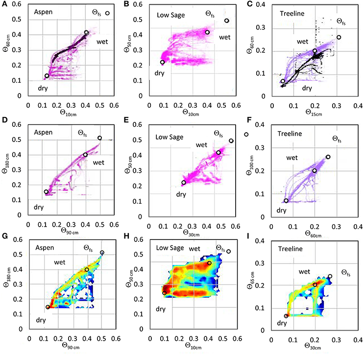
Figure 4. Example plots of Θ data from sensors at different depths in one soil pit each at Aspen and Low Sage and for two pits at Treeline, using a range of sensor depth combinations. Data are shown with the deeper sensor on the y-axis to maintain a counterclockwise hysteresis for all plots. Data markers are semi-transparent to highlight high frequency areas by superposition. Circular data markers are placed at points of maximum frequency corresponding to PEL and FC and maximum values at Θ_fs. As in Figure 3, the highest frequency Θ data values are displayed as circular markers for the dry and wet attractors and Θ_fs. Frames (B,D) are shown as colormaps in frames (G,H). Plot (I) at Treeline pit 4 is displayed for the 30 cm depth analysis due to a failed sensor in pit 3 to compare with pit 3 data in (C,F). Additional data overlays of field tensiometer data (A,C) support later discussion.

Despite differences in soil depth, texture, annual water input from rain and snow, and vegetation cover types, the hysteresis plots for most sites are similar in form, with a few important differences. All hysteresis plots with a near surface measurement (e.g., Figures 2D, 4A–C) show a marked inflection in the drying limb, whereas hysteresis plots for lower depths (e.g. Figures 4D,E) are more triangular, with the constant slope of the drying limb extending to near the dry attractor, indicating more uniform drying across depth. For some sites (e.g., Figure 4F) the hysteresis plot can vary annually between these forms, depending on the timing of precipitation. As a result, the range of the wet attractor over the depth of the soil profile is from 0.13 to 0.08 Θ at Aspen and less (0.02–0.07 Θ) at drier sites such as Low Sage and Treeline (Table 3). Similarly, the distribution of Θ frequency values within the hysteresis loop is quite different among Aspen, Low Sage and Treeline (Figures 4G–I). The differences in the distribution Θ frequency is directly related to differences in depth and timing of precipitation and snowmelt and soil drainage rates for the different soil textures.

TABLE 3

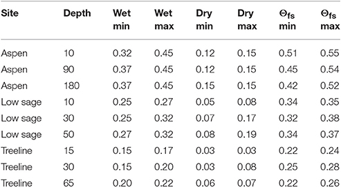
Table 3. Period of study maximum and minimum annual values of wet and dry data attractors (Θ) and Θ_fs for hysteresis analysis at a range of depths (cm) at selected sites.

Figure 5 compares the range of estimated values for Θ_fs(Figure 5A), and the wet (Figure 5B) and dry (Figure 5C) attractors for selected soil depths at the study sites. Data are presented as maxima and minima of all estimates for time series, frequency, paired, and hysteresis analyses. Representative estimated values for each parameter were determined by comparison of the average of annual estimated values to period of record estimated values. Θ_fs values are equated to the maximum Θ found by long term (decadal) frequency analysis (Figure 5A) and exceed average values from the paired and hysteresis analyses by 0.02–0.16 Θ. For the wet and dry attractors, value estimates from the paired and hysteresis analyses are often similar, despite differences in range, both of which are narrower than the value ranges for time series and frequency analyses (Figures 5B,C). The representative estimated value was determined as the most common value among period of record estimate, the average value of annual estimates of paired analyses, and the average value of six period of record hysteresis estimates. This approach generally resulted in a set of values which differed by <0.02 Θ. Context for the results in Figure 5 is provided by Θ estimates at 0 kPa, 33 kPa, and 1.5 MPa for the various soil textures by a commonly used pedotransfer function (Saxton and Rawls, 2006).

FIGURE 5

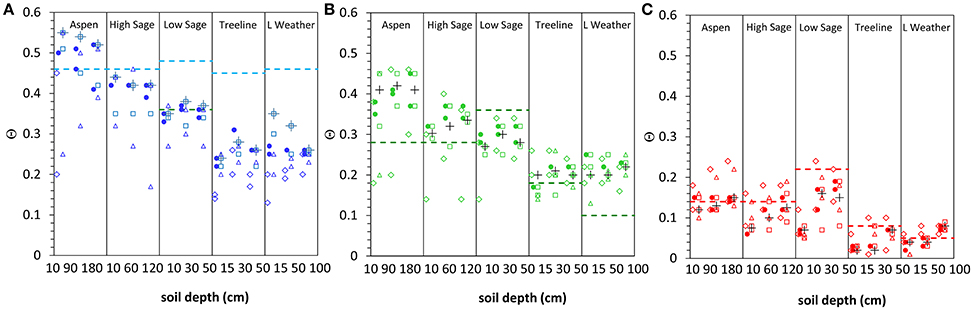
Figure 5. Range of values for Θ_fs (A), wet attractor (B), and dry attractor (C) for three soil depths at the study sites. Data are presented as maxima and minima of all estimates for time series (triangle), frequency (diamond), paired (circle) and hysteresis (square) analyses. Representative estimated values (cross) are shown as point values and Θ estimates at 0 kPa, 33 kPa and 1.5 MPa (dashed lines) for the various soil textures by a commonly used pedotransfer function (Saxton and Rawls, 2006) are provided for context.

The inherent uncertainty in the determining representative attractor values is complicated by physical heterogeneity in soil properties and the somewhat subjective assignment of a single value from within a data attractor that may be weak, have multiple maxima (Figure 4G) or a wide value range (Figure 4H). Figure 6 provides a summary of data attractor results from Figure 5 with the addition of estimated point values of Θ_ws, determined as single values from time series analysis. The Θ_ws values ranged from 0.07 to 0.37 among sites, with the values from Treeline and Lower Weather ranging from 0.06 to 0.10, slightly less than or equal to the values determined by Smith et al. (2011) for sites in Dry Creek watershed. The Θ_ws values ranged from a seven to 38% of the difference between PEL and FC.

FIGURE 6

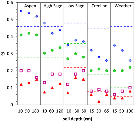
Figure 6. Summary of Θ_fs (blue diamonds), FC (green circles), and PEL (red triangles) values and estimated point values of Θ_ws, (violet squares) by the method of Smith et al. (2011). Results are shown for representative depths at each site and compared to Θ values estimated by a pedotransfer function based on soil texture for 0 kPa (blue dashed line), 33 kPa (green dashed line), and 1500 kPa (red dashed line) by Saxton and Rawls (2006).

Relation of Inferred Values to Physical Measurements

Table 4 compares estimated values of wet and dry attractors to data from soil water retention curves, field tensiometry and an intensive soil irrigation, and drainage experiment. We found that the example dry and wet attractors for Aspen and Treeline sites are equivalent to FC and PEL, respectively. Figure 7 shows the soil water retention curves for Aspen for samples from 1–3 cm (blue) and 41–43 cm (brown) and field tensiometer data at 60 cm (black). The wet attractor Θ values for both depths at Aspen (0.41, 0.41) nearly matched the Θ value (0.42, 0.42) at 10 kPa, commonly used as an approximation of FC. Similarly, the dry attractor Θ values (0.13, 0.13) for both depths at Aspen nearly matched the 1.5 MPa Θ values (0.12, 0.12). For Treeline at 60 cm the hysteresis method wet attractor Θ (0.21) compares well with the measured Θ (0.19) corresponding to a tensiometer value of 10 kPa. Although, not exhaustive, this evidence strongly supports the hypothesis that data attractors represent FC and PEL, and that other important soil hydrologic parameters can be determined from Θ records for sites with different soils, wetness and plant cover.

TABLE 4

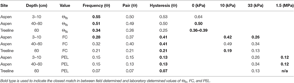
Table 4. Comparison of estimated values of soil hydrologic parameters Θ_fs, FC, and PEL from Θ records by frequency, paired sensors, and hysteresis methods to Θ-values corresponding to common soil water potentials used in laboratory experiments.

FIGURE 7

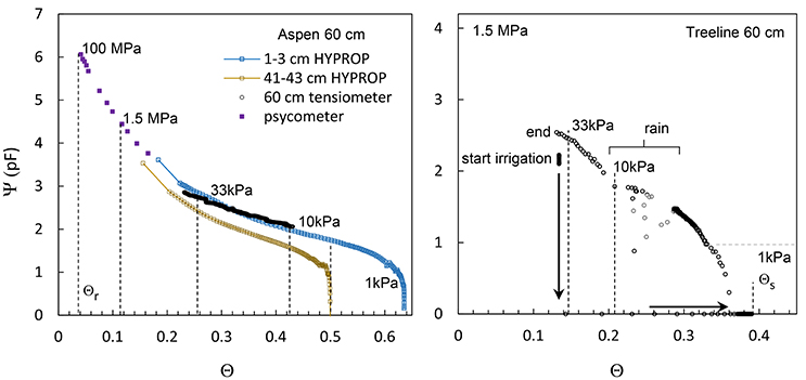
Figure 7. Soil moisture characteristic curve measurements for Aspen site (60 cm), samples from similar silt loam sites in RCEW, and sandy loam at Treeline site (60 cm). Soil water tension values are shown as pF, (log hPa) and identified on the curves at 10, 33, and 1,500 kPa as vertical gray lines in both panels. Measurements for the silt loam include Aspen site 60 cm field tensiometer (black) and laboratory measurement by psychrometer (violet) and HYPROP at 0–2 cm (brown) and 41–43 cm (blue) for silt loam samples from a similar site nearby Aspen. Measurements for Treeline site sandy loam are shown for a prior experiment to determine FC that was interrupted by a period of rain. Laboratory and model estimates for Θr are soil samples from 24 to 25 cm depth (Gribb et al., 2009). Values determined by Θ frequency analyses are shown as black dashed lines in both panels. A range of relatively high frequency data greater than FC are shown to indicate the range of estimates in this value by various methods.

Additional inspection of Figure 7 and results from the frequency analysis of Θ are presented here to clarify the interpretation of Θ_s, and Θ_fs. For the Aspen the laboratory saturated (0 kPa) Θ ranges from Θ_s of 0.64 at 1–3 cm to 0.50 at 41–43 cm depth. The frequency method estimated value of Θ_fs at 10 cm depth (0.55) falls between these values and is substantially less than Θ_s for the soil surface measurement. This difference is likely due to either a decrease in soil porosity between 2 and 10 cm depth or a difference between Θ at Θ_s and Θ_fs. At greater depth the difference between the frequency method value for Θ_fs at 60 cm (0.51) and the value at for 0 kPa at 41–43 cm (0.50) is negligible, indicating Θ_fs is equivalent to Θ_s at these depths. For sandy soils at Treeline, constant irrigation achieved Θ_s at 60 cm (Θ = 0.39) and upon drainage, the air entry value (0.36) was similar to Θ_fs (0.34) as determined by the frequency method.

Discussion

The objectives of this paper are to evaluate four approaches to determine if temporal patterns of measured soil water values are consistent with the concepts of Θ_s, FC, PEL, and Θ_ws. The method exploits the increasing availability of electronic soil water data to address the considerable controversy, both theoretical and conceptual, regarding soil water content constants. We found good agreement between soil hydrologic parameter values determined from attractors found in in situ Θ sensor records and from conventional laboratory techniques, for a limited number of samples representing sandy loam and silt loam soils (Figure 7). These results support the hypothesis that data attractors represent FC and PEL, and that other important soil hydrologic parameters can be determined from Θ records for sites with different soils, wetness, and plant cover. We demonstrate the results of the analyses by overlaying the representative parameter values on the time series data from which the values were derived (Figure 8) to support discussion of the determination of values for various soil hydrologic properties, applicability of this approach to other sites and caveats for use where frozen soils occur. In the following sections we comment on the value of the approaches for estimating each property (Θ_s, FC, PEL, and Θ_ws), followed by a discussion of uncertainty and errors.

FIGURE 8

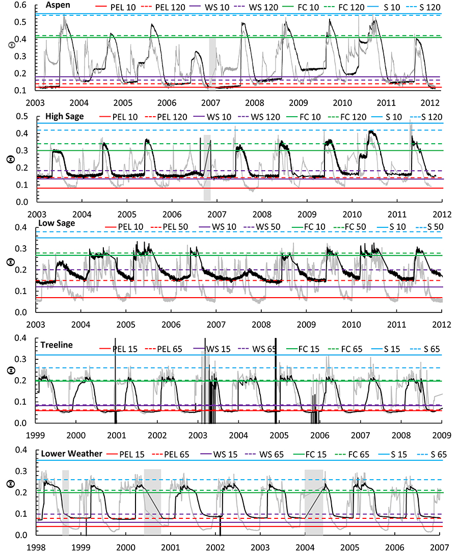
Figure 8. Time series data and parameter values determined by frequency analysis for Θ_fs (blue lines), hysteresis analysis for FC (green lines), and PEL (red lines), and time series analysis for Θ_ws (violet lines). Depth of measurements are indicated in each panel for the shallow (gray) and deep (black) sensor locations.

Saturation (Θ_s)

Saturation was uncommon in our data. All of the study sites are well-drained and did not show evidence of a water table. Therefore, it is not surprising that we found no attractor around saturation. However, near surface soil pipes and macropores may intermittently fill and appear as data outliers. This may explain why the maximum measured values of Θ can be quite different from the pedotransfer function estimates of saturation, especially near the soil surface. Results from our analyses for Aspen and Treeline sites show maximum Θ (Θ_fs) values of 0.55, 0.51, and 0.34 (Table 4) from controlled experiments and values of 0.64, 0.50, and 0.39 from field measurements. The difference in peak saturation for shallow soil at Aspen may arise from differences in porosity between the surface 3 cm and at 10 cm depth, or the greater capacity for occluded soil gas below the very dense mat of fine roots within above the mineral soil. We note that complete saturation of soils requires extensive irrigation, either in the field (Ellis and Lee, 1919; Hillel et al., 1972) or laboratory (Hazen, 1892; Watson, 1966) to ensure near complete removal of gas from the soil pores. Analysis of both laboratory and field measurements should be repeated for multiple depths in the soil profile.

At most sites, field saturation, Θ_fs, is a transient state achieved during infrequent periods of high flux and can range from FC to Θ_s in annual records (Figure 8). Assuming a consistent pore size distribution over time, it is logical to select the greatest recorded in situ value as Θ_fs either as a tail of the frequency analysis over the period of record. This selection requires judgment to determine if the extreme value is a valid measurement point or an artifact of measurement. This is likely an appropriate proxy value (Figure 5A) for most modeling purposes as long as the site remains freely draining. Θ_fs decreases with depth for all sites except Low Sage (which had a strong textural contrast), presumably in response to decreased porosity, decreased organic matter increased occluded volume by gravel or attenuation of flux by storage. These effects are lumped by the approach presented here. Due to the dependence of Θ on flux for well-drained sites, determination of Θ_fs is likely improved with longer data series and shorter time step data, especially for semi-arid or drier sites.

Field Capacity (FC)

The most consistent representation of FC often corresponded with the intersection of the wetting and drying limbs of the hysteresis loops (Figure 2D) and near the low edge of the wet data attractor in the paired analysis, as shown for Aspen and Treeline (Figure 3). These constraints on selection of FC recognize that this attractor requires that soil wetting is followed by a period of several days with no evaporation. Therefore, FC is most evident after cool season precipitation events, which are dominant in the study environment. During snowmelt, radiation and temperature patterns drive diel fluctuations of melt water flux to the soil that can to lead to positive bias in estimation of FC.

We found very similar values for FC at all depths within Aspen, Treeline, and Lower Weather but variability in FC with depth at High Sage and Low Sage (Figure 6). Although, texture is a first-order control on FC, the values from our analyses were often quite different from the pedotransfer function predictions, and even the same texture: FC at High Sage ranges from 74 to 82% of FC at Aspen for the surface and deep sensors, respectively, which is remarkable, given the close proximity and nearly identical soils at these sites. The difference in attractor values between Aspen and High Sage is due to the different soil water input environments. Aspen site is located beneath a seasonal snow drift that is typically 3 m deep. This results in extended periods during which daily water inputs from snowmelt maintain soil water contents at values greater than FC. Winter snow cover at High Sage site is typically 50 cm. It therefore melts much earlier and is subject to periodic cool season rainfall events that allow for drainage to FC, thus shifting the attractor downward to a value more consistent with the concept of FC. The pedotransfer function predictions appear reasonable (with hindsight) for sites other than Aspen (Figure 6), but appear to correspond better to Θ_fs values presented for Low Sage and Treeline. These differences in representation of the mobile water fraction in soil are likely attributable to soil plant interactions such as litter cover and secondary soil structure and are important for careful parameterization for ecohydrological models.

Plant Extraction Limit (PEL)

PEL, like Θ_ws is an ecohydrologic parameter that represents an interaction among plant phenology, the surface energy balance, and soil water potential. For this study, the land surface cover is dominated by perennial vegetation with varying extent of litter and bare soil across sites, soil water input is primarily derived from spring snowmelt resulting in an extended dry growing season, and peak PET is in July (Seyfried et al., 2011). These conditions, in conjunction with the low mean annual precipitation outside of snow drifts all facilitate very dry soil states required for development of an attractor at PEL. The dry attractor values in this study were generally slightly less than those predicted by the pedotransfer function, and converse from Θ_fs, tended to increase with depth.

Our initial premise was that PEL at any depth is represented by a constant value of Θ for an extended period during the growing season, as shown for Treeline and Low Sage (Figure 8). For other sites, PEL may not be consistently represented across years for either the shallow or deep sensors for two reasons: First, Aspen is often energy limited and retains water at depth in most years, only achieving PEL in 2003, 2007, and 2012 (Figure 8). Similarly, other sites with insufficient energy to evaporate the mean annual precipitation are unlikely to reach PEL at depth. Second, Θ less than PEL commonly occurs in near surface soils. Records from Treeline and Lower Weather show Θ as low as 0.01 for sensors at 5 cm depth, but a PEL of 0.06 to 0.08 at depth (Figure 8). Evaporative drying near the soil surface can decrease Θ below PEL. In this case, when the evaporative potential at the leaf surface is balanced or exceeded by soil water tension, plant water use is negligible and vapor diffusion governs evaporation (Buckingham, 1907; Salvucci, 1997). This transition from viscous capillary (S1) to vapor diffusion (S2) control on evaporation (Brutsaert and Chen, 1995; Lehmann et al., 2008) is apparent in data, and complicates the interpretation of the dry attractor and PEL.

Thus, interpretation of the range of the dry attractor requires consideration, as with the wet attractor. Lower Weather receives the greatest energy and least precipitation among the study sites, and has coarse textured soils with a nearly bare surface, making it a good case study for dry soils. Initial estimates of the dry attractor Θ range from 0.04 at 15 cm to 0.08 at 100 cm (Figure 8). The much lower values of the dry attractor for 5 cm sensors at 0.00 < Θ < 0.02 (Figure 8) likely represents the limit of evaporation via vapor diffusion near the surface, for the available seasonal energy. We found a gradient 0.00 < Θ < 0.08 develops from 5 to 100 cm depth in response to the vapor diffusion gradient above PEL at 100 cm depth. These observations lead to the conclusion that near the soil surface, the shift from evapotranspiration to evaporation below PEL is difficult to distinguish using a data attractor.

Plant Water Stress (Θ_ws)

Important features of soil drying below FC include the initiation of plant water stress, Θ_ws, the endpoint of plant water use, PEL, and the transition to evaporative drying by vapor diffusion. We found that the semi-arid climate of the study sites provided ideal conditions for soil drying through spring and summer, as shown by a nearly constant drying trend over approximately the middle half of the range in Θ for all sites (except Low Sage). Yet, a notable difference is evident between drying patterns for shallow and deep sensor locations: Soils at depths of 15 cm or less dried first and fastest at near steady state from below FC to near PEL (Figure 8). For soils below 15 cm the drying function Θ(t) was quasi-sinusoidal between FC and PEL, with a shift to faster drying when the shallow sensor reached Θ_ws. We attribute this initial increase in the rate of deep soil drying to consistent (energy-limited) plant water use from a smaller storage volume following surface drying below Θ_ws. For all sites, Θ_ws occurred annually for the shallow sensor depths, but was less consistent for the deep sensors. For example, Θ records from the deep sensors Aspen and High Sage regularly show linear declines until approximately Oct 1, when the water year ends with the onset of freezing nighttime air temperatures and abrupt termination of plant water use at these high elevation sites, e.g., WY 2008–2010 (Figure 8). Thus, as Θ_s may not be consistently achieved due to surface infiltration rates that seldom exceed soil profile drainage flux, Θ_ws may not be consistently achieved due to insufficient seasonal energy. Yet, the occasional dry years (e.g., WY 2006) at Aspen and High Sage are clearly water limited and are sufficient to estimate Θ_ws for the high elevation sites. Low Sage and the lower, elevation Treeline and Lower Weather sites are annually water limited and show consistent inflections indicating Θ_ws during July and August with values ranging from 0.20 for the deep clay soils at Low Sage to 0.07 for deep soils at Treeline (Figures 6, 8).

Uncertainty and Errors

One approach to the uncertainty in evaluating contemporaneous soil moisture states is to visualize Θ(z) at a daily to weekly time step. Figure 9 shows Θ(z) for wetting and drying periods over one water year at Aspen and Treeline. Although, this approach is somewhat difficult to implement over multiple years, it provides insight on the gradation of soil hydrologic properties with depth and the different dynamics of wetting and drying across sites. This type of diagram is common in texts, but typically focuses attention on the dynamics of wetting and drying, rather than the predominant soil moisture states. For both sites, a vertical profile at FC emerges after the wetting front arrives at the base of the soil. Yet Θ(z) may not reach Θ_fs, as determined from the long term record for any depth in a given year. During soil drying, similar increasing gradients in Θ(z) emerge slightly below FC at both sites in response to plant water use, and indicate a rapid decline in drying associated with Θ_ws, near PEL. The much sharper inflection in Θ(z) near the soil surface at Treeline than Aspen reflects the difference in surface evaporation between sites. Finally, the much broader band of overlap among Θ(z) profiles at Treeline reflects the longer period and greater depth of plant water stress at that site.

FIGURE 9

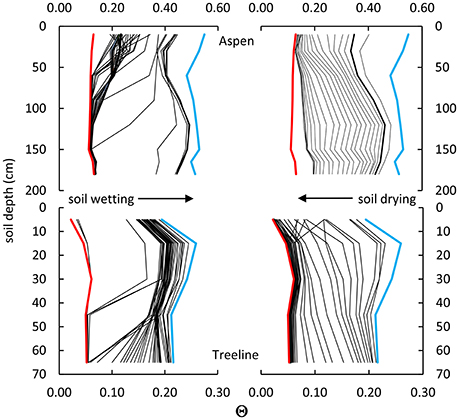
Figure 9. Soil moisture profile sequences for Aspen (top) and Treeline (bottom), showing wetting (left), and drying sequences (right). Five-day interval profiles are shown in black and extreme values of dry (red) and wet (blue) conditions at each soil depth. Attractor Θ values for Aspen (near 0.40) and Treeline (near 0.20) over the depth of the soil profiles emerge where there is substantial overlap in the 5-day interval lines in the wetting sequence for both sites, following wetting of deep soils. Similar overlap occurs for Θ as a function of depth for PEL, which ranges from near 0.07 to 0.10 for Aspen and 0.05–0.07 for Treeline.

Each approach to determining soil hydrologic properties has a different bias, but all are in general agreement. The applicability of measured data for this model parameterization depends on the nature of soil water dynamics under consideration. Selection of specific values for the wet and dry attractors by time series analysis is more subjective than by frequency analysis, as it depends on selection of a single value from a range of Θ near the extreme values. The two depth hysteresis method provides estimates that closely match the Θ at standard soil water potential values commonly used to define FC and PEL. The improvement over the other methods for determining these wet and dry attractors is related to the reduced overlap between valid data, and the invalid data and data errors which can skew the frequency distribution of the attractor. In particular, the juxtaposition of Θ for a sensor depth (a) with stable Θ to a sensor at a different depth (b) with either increasing or decreasing Θ develops a linear trace toward a point of inflection where the rate of change in sensor a increases and sensor b decreases. The relatively slow rate of change near the inflection enhances the frequency of (a,b) data at the attractor. Error values tend to fall at the margins of the hysteresis loop which reduces error distortion of the main attractors (e.g., Figure 4). Unlike the hysteresis analysis, the paired sensor approach can also be biased by any temporal lag in wetting front depth between the sensors.

Soil depth and cover effects are clearly represented in the presented analyses. We found the sites with very well drained soils (Treeline, Lower Weather) showed less uncertainty in Θ_fs and FC near the bottom of the soil profile (Figure 5), likely as a result of faster transit times and less retention. Similarly, the control of surface cover on evaporation is clearly represented in general across sites. PEL is not strictly a soil property, but also depends on vegetation where roots are active. The soil at High Sage has the same texture as Aspen, but the surface cover is dense shrub canopy 0.5–1.5 m over with 2–5 cm of litter and bare interspace and associated decreasing values of PEL at 60 cm (0.10) and 10 cm (0.08). This cover appears to effectively limit surface evaporation. Low Sage has a soil textural gradient from silt loam to clay loam and a bare soil surface and results in the strongest gradient in PEL (0.07–0.14) over the least depth of soil, 50 cm. Treeline and Lower Weather are both sandy sites with shrub cover and low bulk density surface, which supports extensive drying. Difference in PEL following vegetation removal by prescribed fire in 2007 are clear at the Aspen and High Sage sites.

There are two primary effects. First, electronic soil water sensors are based on relating measured permittivity to liquid water content, which is generally a robust relationship because the permittivity of liquid water (80) is so much greater than soil (5) or air (1). However, the permittivity of ice (3.1) is very similar to that of air, so frozen soil appears to have less water content and effectively approximates the liquid water content of the soil (Seyfried and Murdock, 1996). This effect is apparent when dramatic “drying” events during the winter appear as noise and stray from the FC attractor. Freezing effects are apparent in all four panels in Figure 2 and can be clearly seen by comparison of the soil moisture trends at 15 cm and 30 cm in Figure 9. Second, freezing effectively reduces the soil water potential. When the near-surface soil freezes, the normal downward hydraulic gradient is reversed and water moves upward toward the freezing front. This can cause either an increase or decrease in the measured soil water content, depending on the proximity of the sensor to the freezing front (Hillel, 1980). These are most pronounced near the soil surface, which commonly freezes in this environment. In this study the freezing front rarely exceeded 30 cm. There is evidence of occasional upward gradient effects apparent deeper in the soil profile. These artifacts can introduce erroneous data into the analysis. This is more problematic for the frequency and paired analyses, in which the surface sensors are likely to be similarly affected, but less important for the hysteresis analysis. We suggest that soil temperature records, which are commonly collected along with TDR or other soil moisture measurements, could be used to censor data during periods of soil frost prior to conducting the presented analyses.

Conclusions

We demonstrate a novel approach to extract important soil hydrologic parameters directly from field data. The approach takes advantage of the increasing availability of continuously monitored Θ. Because it is based on in-situ data, results are directly related to the local climate, soils and vegetation and does not rely on assumed pedotransfer functions or proxy measurements such as Ψ. The approach builds primarily on concepts of Θ_s, FC, and PEL inherited from irrigated agriculture, but regards these quantities in terms of the amount of water retained in the soil, rather than in terms of soil water potentials. This approach is consistent with mass-based modeling schemes and provides detail for estimation of other additional transitional and extreme states Θ_fs, Θ_ws. However, the applicability of measured data for this model parameterization depends on the nature of soil water dynamics under consideration. The implicit assumptions are that drainage from Θ_s or Θ_fs to FC is relatively fast in the absence of soil water input, and below that threshold 1D unsaturated flow responds primarily to plant water uptake, which decreases progressively below Θ_ws and ceases at PEL. The endpoint of drying in any annual cycle may range from a value greater than PEL to Θ_r, depending on plant type and soil texture and depth. These assumptions are supported by observations and data from the sites in this study, which indicate a downward wetting front progression for every major rainfall or snow melt and the regular and extensive periods of soil wetting and drying. Application of the developed approach in more humid climates, or in the presence of a persistent phreatic surface is expected to improve estimation of Θ_s, but may provide little guidance on PEL or Θ_ws. Preferential flow is not specifically addressed, but the non-unity slopes in the paired analysis indicate that variable rates of wetting front advance can complicate interpretation of this approach. Similarly, vertical bypass flow in individual sensor profiles may complicate interpretation of FC and Θ_ws, but not PEL.

We found that the frequency of measured values tended to be greatest around observable “attractors” that correspond to the specific hydrologic parameters of interest. Of the four approaches analyzed, we found the hysteresis analysis approach is the most robust predictor of data attractors and frequency analysis is the simplest approach to determine the extreme values. Nevertheless, we consider the construction of a two dimensional Θ frequency matrix as the most effective and practical single approach to parameter value identification. This approach enables analysis from a single profile of sensors and provides the greatest visual support to estimate parameter values. The data and analyses presented here clearly demonstrate how near surface Θ often differs from the deeper soil at many sites, due to differences in macroporosity, soil freezing, hysteresis in wetting. These controls on soil profile storage may confound attempts to measure soil profile storage by remote sensing methods, and opportunities to overcome some of these obstacles will be addressed in a successive paper.

Author Contributions

DC: Conceived research concept and analyses, conducted fieldwork, was primary author. MS: Contributed to research concept, conducted fieldwork and laboratory experiments, was second author. JM: Contributed to research concept, conducted fieldwork, contributing author. KH: Conceived research concept and analyses.

Conflict of Interest Statement

The authors declare that the research was conducted in the absence of any commercial or financial relationships that could be construed as a potential conflict of interest.

Acknowledgments

The authors would like to thank two reviewers who provided extensive and valuable comments to the manuscript and finding from USDA NRI Grant 2001-35102-11031, USDA SGP award 2005-34552-15828.

References

Assouline, S., and Or, D. (2014). The concept of field capacity revisited: defining intrinsic static and dynamic criteria for soil internal drainage dynamics. Water Resour. Res. 50, 4787–4802. doi: 10.1002/2014WR015475

CrossRef Full Text | Google Scholar

Bandara, R., Walker, J. P., and Rüdiger, C. (2013). Towards soil property retrieval from space: a one-dimensional twin-experiment. J. Hydrol. 497, 198–207. doi: 10.1016/j.jhydrol.2013.06.004

CrossRef Full Text | Google Scholar

Boote, K. J., Sau, F., Hoogenboom, G., and Jones, J. W. (2008). “Experience with water balance, evapotranspiration, and predictions of water stress effects in the CROPGRO model,” in Response of Crops to Limited Water: Understanding and Modeling Water Stress Effect on Plant Growth Processes, eds R. Ahuja, V. R. Reddy, S. A. Saseendran, and Q. Yu (Madison, WI: American Society of Agronomy), 59–103.

Google Scholar

Briggs, L. J., and McLane, J. W. (1907). The moisture equivalent of soils. U.S. Dept. Agr. Bur. Soils Bul. 46, 1–23.

Briggs, L. J., and Shantz, H. L. (1912). The wilting coefficient for different plants and its indirect determination. Bot. Gaz. 53, 20–37. doi: 10.5962/bhl.title.64958

CrossRef Full Text

Brooks, R. H., and Corey, A. T. (1964). Hydraulic properties of porous media and their relation to drainage design. Trans. ASAE 7, 26–28. doi: 10.13031/2013.40684

CrossRef Full Text | Google Scholar

Brutsaert, W., and Chen, D. (1995). Desorption and the two stages of drying of natural tallgrass prairie. Water Resour. Res. 315, 1305–1313. doi: 10.1029/95WR00323

CrossRef Full Text | Google Scholar

Buckingham, E. (1907). Studies on the Movement of Soil Moisture, Bureau of Soils, Bulletin 38. Washington, DC: U.S. Department of Agriculture.

Budyko, M. I. (1956). Heat Balance of the Earth's Surface. Leningrad: Gidrometeoizdat.

Google Scholar

Burdine, J. A., and Redford, E. S. (1952). Selected articles and documents on american government and politics. Am. Polit. Sci. Rev. 46, 254–257. doi: 10.1017/S0003055400069239

CrossRef Full Text | Google Scholar

Cassel, D. K., and Nielsen, D. R. (1986). “Field capacity and available water capacity,” in Methods of Soil Analysis: Part 1—Physical and Mineralogical Methods, ed A. Klute (Madison, WI: American Society of Agronomy and Soil Science Society of America), 901–926.

Google Scholar

Chandler, D. G., Seyfried, M., Murdock, M., and McNamara, J. P. (2004). Field calibration of water content reflectometers. Soil Sci. Soc. Am. J. 68, 1501–1507. doi: 10.2136/sssaj2004.1501

CrossRef Full Text | Google Scholar

Chauvin, G. M., Flerchinger, G. N., Link, T. E., Marks, D., Winstral, A. H., and Seyfried, M. S. (2011). Long-term water balance and conceptual model of a semi-arid mountainous catchment. J. Hydrol. 400, 133–143. doi: 10.1016/j.jhydrol.2011.01.031

CrossRef Full Text | Google Scholar

Colman, E. A. (1947). A laboratory procedure for determining the field capacity of soils. Soil Sci. 63, 277–283. doi: 10.1097/00010694-194704000-00003

CrossRef Full Text | Google Scholar

Cuenca, R. H., Ek, M., and Mahrt, L. (1996). Impact of soil water property parameterization on atmospheric boundary layer simulation. J. Geophys. Res. Atmos. 101, 7269–7277. doi: 10.1029/95JD02413

CrossRef Full Text | Google Scholar

Damesin, C., and Rambal, S. (1995). Field study of leaf photosynthetic performance by a Mediterranean deciduous oak tree (Quercus pubescens) during a severe summer drought. New Phytol. 131, 159–167. doi: 10.1111/j.1469-8137.1995.tb05717.x

CrossRef Full Text | Google Scholar

Ellis, A. J., and Lee, E. H. (1919). Geology and Ground Waters of the Western Part of San Diego County, California. Water Supply Paper, U.S. Geology Survey, 23–24.

Fayer, M. J., and Hillel, D. (1986). Air encapsulation: I. Measurement in a field soil. Soil Sci. Soc. Am. J. 50, 568–572 doi: 10.2136/sssaj1986.03615995005000030005x

CrossRef Full Text | Google Scholar

Flerchinger, G. N., Cooley, K. R., Hanson, C. L., and Seyfried, M. S. (1998). A uniform versus an aggregated water balance of a semi-arid watershed. Hydrol. Process. 12, 331–342. doi: 10.1002/(SICI)1099-1085(199802)12:2<331::AID-HYP580>3.0.CO;2-E

CrossRef Full Text | Google Scholar

Flerchinger, G. N., Marks, D., Reba, M. L., Yu, Q., and Seyfried, M. S. (2010). Surface fluxes and water balance of spatially varying vegetation within a small mountainous headwater catchment. Hydrol. Earth Syst. Sci. 14, 965–978. doi: 10.5194/hess-14-965-2010

CrossRef Full Text | Google Scholar

Grayson, R. B., Western, A. W., Walker, J. P., Kandel, D. G., Costelloe, J. F., and Wilson, D. J. (2006). “Controls on patterns of soil moisture in arid and semi-arid systems,” in Dryland Ecohydrology, eds P. D'Odorico and A. Porporato (Dordrecht: Springer), 109–127.

Google Scholar

Gribb, M. M., Forkutsa, I., Hansen, A., Chandler, D. G., and McNamara, J. P. (2009). The effect of various soil hydraulic property estimates on soil moisture simulations. Vadose Zone J. 8, 321–331. doi: 10.2136/vzj2008.0088

CrossRef Full Text | Google Scholar

Hansen, V. E., Israelsen, O. W., and Stringham, G. E. (1980). Irrigation Principles and Practices, 4th Edn. New York, NY: Wiley.

Hazen, A. (1892). Experiments upon the Purification of Sewage and Water at the Lawrence Experiment Station. Massachusetts State Board Health, Twenty-third Annual Report for 1891, Wright & Potter, Printing Co.

Google Scholar

Hillel, D. (1980). Applications of Soil Physics. New York, NY: Academic Press.

Hillel, D., Krentos, V. D., and Stylianou, Y. (1972). Procedure and test of an internal drainage method for measuring soil hydraulic characteristics in situ. Soil Sci. 114, 395–400. doi: 10.1097/00010694-197211000-00011

CrossRef Full Text | Google Scholar

Huang, X., Shi, Z. H., Zhu, H. D., Zhang, H. Y., Ai, L., and Yin, W. (2016). Soil moisture dynamics within soil profiles and associated environmental controls. Catena 136, 189–196. doi: 10.1016/j.catena.2015.01.014

CrossRef Full Text | Google Scholar

Idso, S. B., Reginato, R. J., Jackson, R. D., Kimball, B. A., Nakayama, F. S., et al. (1974). The three stages of drying of a field soil. Soc. Am. Proc. 38, 831–836.

Google Scholar

Kirkham, M. B. (2005). Principles of Soil and Plant Water Relations. San Diego, CA: Academic Press.

Google Scholar

Kormos, P. R., Marks, D., Williams, C. J., Marshall, H. P., Aishlin, P., and Chandler, D. G. (2014). Soil, snow, weather, and sub-surface storage data from a mountain catchment in the rain–snow transition zone. Earth Syst. Sci. Data 6, 165–173. doi: 10.5194/essd-6-165-2014

CrossRef Full Text | Google Scholar

Koster, R. D., Dirmeyer, P. A., Guo, Z. C., Bonan, G., Chan, E., Cox, P., et al. (2004). Regions of strong coupling between soil moisture and precipitation. Science 305, 1138–1140. doi: 10.1126/science.1100217

PubMed Abstract | CrossRef Full Text | Google Scholar

Koster, R. D., Schubert, S. D., and Suarez, M. J. (2009). Analyzing the concurrence of meteorological droughts and warm periods, with implications for the determination of evaporative regime. J. Clim. 22, 3331–3341. doi: 10.1175/2008JCLI2718.1

CrossRef Full Text | Google Scholar

Laio, F., Porporato, A., Ridolfi, L., and Rodriguez-Iturbe, I. (2001). Plants in water-controlled ecosystems: active role in hydrologic processes and response to water stress: II. Probabilistic soil moisture dynamics. Adv. Water Resour. 24, 707–723. doi: 10.1016/S0309-1708(01)00005-7

CrossRef Full Text | Google Scholar

Lehmann, P., Assouline, S., and Or, D. (2008). Characteristics lengths affecting evaporative drying from porous media. Phys. Rev. E 77:056309. doi: 10.1103/PhysRevE.77.056309

PubMed Abstract | CrossRef Full Text | Google Scholar

Liang, X., Wood, E. F., and Lettenmaier, D. P. (1996). Surface soil moisture parameterization of the VIC-2L model: evaluation and modification. Global Planet. Change 13, 195–206. doi: 10.1016/0921-8181(95)00046-1

CrossRef Full Text | Google Scholar

Linsley, R. K., and Franzini, J. B. (1972). Water Resources Engineering. New York, NY: McGraw-Hill.

Loik, M. E., Breshears, D. D., Laurenroth, W. K., and Belnap, J. (2004). A multi-scale perspective of water pulses in dryland ecosystems: climatology and ecohydrology of the western USA. Oecologia 141, 269–281. doi: 10.1007/s00442-004-1570-y

PubMed Abstract | CrossRef Full Text | Google Scholar

Marinas, M., Roy, J. W., and Smith, J. E. (2013). Changes in entrapped gas content and hydraulic conductivity with pressure. Ground Water 51, 41–50. doi: 10.1111/j.1745-6584.2012.00915.x

PubMed Abstract | CrossRef Full Text | Google Scholar

McNamara, J. P., Chandler, D., Seyfried, M., and Achet, S. (2005). Soil moisture states, lateral flow, and streamflow generation in a semi-arid, snowmelt-driven catchment. Hydrol. Process. 19, 4023–4038. doi: 10.1002/hyp.5869

CrossRef Full Text | Google Scholar

Meinzer, O. E. (1923). Outline of Ground-Water Hydrology, with Definitions. United States Geological Survey, Water Supply Paper 494, p. 29.

Google Scholar

Metzger, T., and Tsotsas, E. (2005). Influence of pore size distribution on drying kinetics: a simple capillary model. Drying Technol. 23, 1797–1809. doi: 10.1080/07373930500209830

CrossRef Full Text | Google Scholar

Miller, R. D., and McMurdie, J. L. (1953). Field capacity in laboratory columns. Soil Sci. Soc. Am. J. 17, 191–195. doi: 10.2136/sssaj1953.03615995001700030003x

CrossRef Full Text | Google Scholar

Miller, E. E., and Klute, A. (1967). “The dynamics of soil water: part I—mechanical forces,” in Irrigation of Agricultural Lands, eds R. M. Hagan, H. R. Haise, and T. W. Edminster (Madison, WI: American Society of Agronomy), 209–244.

Google Scholar

Montzka, C., Moradkhani, H., Weihermüller, L., Franssen, H.-J. H., Canty, M., and Vereecken, H. (2011). Hydraulic parameter estimation by remotely-sensed top soil moisture observations with the particle filter. J. Hydrol. 399, 410–421. doi: 10.1016/j.jhydrol.2011.01.020

CrossRef Full Text | Google Scholar

Morse, J. L., Duran, J., Beall, F., Enanga, E. M., Creed, I. F., Fernandez, I., et al. (2015). Soil denitrification fluxes from three northeastern North American forests across a range of nitrogen deposition. Oecologia 177, 17–27. doi: 10.1007/s00442-014-3117-1

PubMed Abstract | CrossRef Full Text | Google Scholar

Mualem, Y. (1976). A Catalogue of the Hydraulic Properties of Unsaturated Soils. Haifa: Technion, Israel Institute of Technology, Technion Research & Development Foundation.

Google Scholar

Nayak, A., Chandler, D. G., Marks, D., McNamara, J. P., and Seyfried, M. (2008). Correction of electronic record for weighing bucket precipitation gauge measurements. Water Resour. Res. 44:W00D11. doi: 10.1029/2008WR006875

CrossRef Full Text | Google Scholar

Nemes, A., Pachepsky, Y. A., and Timlin, D. J. (2011). Towards improving global estimates of field soil water capacity. Soil Sci. Soc. Am. J. 75, 807–812. doi: 10.2136/sssaj2010.0251

CrossRef Full Text | Google Scholar

Njoku, E. G., Jackson, T. J., Lakshmi, V., Chan, T. K., and Nghiem, S. V. (2003). Soil moisture retrieval from AMSR-E. IEEE Trans. Geosci. Remote Sens. 41, 215–229. doi: 10.1109/TGRS.2002.808243

CrossRef Full Text | Google Scholar

Or, D., Lehmann, P., and Assouline, S. (2015). Natural length scales define the range of applicability of the Richards equation for capillary flows. Water Resour. Res. 51, 7130–7144. doi: 10.1002/2015WR017034

CrossRef Full Text | Google Scholar

Osakabe, Y., Osakabe, K., Shinozaki, K., and Tran, L.-S. P. (2014). Response of plants to water stress. Front. Plant Sci. 5:86. doi: 10.3389/fpls.2014.00086

PubMed Abstract | CrossRef Full Text | Google Scholar

Paniconi, C., and Putti, M. (2015). Physically based modeling in catchment hydrology at 50: survey and outlook. Water Resour. Res. 51, 7090–7129. doi: 10.1002/2015WR017780

CrossRef Full Text | Google Scholar

Piper, J. R. (1933). Notes on the relation between the moisture-equivalent and the specific retention of water-bearing materials. EOS Trans. AGU 14, 481–487. doi: 10.1029/tr014i001p00481

CrossRef Full Text | Google Scholar

Prasad, R., Tarboton, D. G., Liston, G. E., Luce, C. H., and Seyfried, M. S. (2001). Testing a blowing snow model against distributed snow measurements at Upper Sheep Creek, Idaho, United States of America. Water Resour. Res. 37, 1341–1356. doi: 10.1029/2000WR900317

CrossRef Full Text

Rambal, S., Ourcival, J. M., Joffre, R., Mouillot, F., Nouvellon, Y., Reichstein, M., et al. (2003). Drought controls over conductance and assimilation of a Mediterranean evergreen ecosystem: scaling from leaf to canopy. Glob. Chang. Biol. 9, 1813–1824. doi: 10.1111/j.1365-2486.2003.00687.x

CrossRef Full Text | Google Scholar

Reichle, R. H., Koster, R. D., Liu, P., Mahanama, S. P. P., Njoku, E. G., and Owe, M. (2007). Comparison and assimilation of global soil moisture retrievals from the Advanced Microwave Scanning Radiometer for the Earth Observing System (AMSR-E) and the Scanning Multichannel Microwave Radiometer (SMMR). J. Geophys. Res. 112:D9. doi: 10.1029/2006jd008033

CrossRef Full Text

Reynolds, W. D., Elrick, D. E., Youngs, E. G. H., Booltink, W. G., and Bouma, J. (2002). “Saturated and field saturated water fl ow parameters,” in Methods of Soil Analysis, Part 4. Physical Methods, SSSA Book Series No. 5., eds J. H. Dane and G. C. Topp (Madison, WI: SSSA), 802–816.

Google Scholar

Richards, L. A., and Weaver, L. R. (1944). Moisture retention by some irrigated soils as related to soil-moisture tension. J. Agric. Res. 69, 215–235.

Google Scholar

Rodriguez-Iturbe, I., D'Odorico, P., Porporato, A., and Ridolfi, L. (1999). On the spatial and temporal links between vegetation, climate, and soil moisture. Water Resour. Res. 35, 3709–3722. doi: 10.1029/1999WR900255

CrossRef Full Text | Google Scholar

Rodriguez-Iturbe, I., Porporato, A., Laio, F., and Ridolfi, L. (2001). Plants in water-controlled ecosystems: active role in hydrologic processes and response to water stress: I. Scope and general outline. Adv. Water Res. 24, 695–705. doi: 10.1016/S0309-1708(01)00004-5

CrossRef Full Text | Google Scholar

Romano, N., and Santini, A. (2002). “Field water capacity,” in Methods of Soil Analysis: Part 4-Physical Methods, eds J. H. Dane and G. C. Topp (Madison, WI: Soil Science Society of America), 722–738.

Salter, P. J., and Haworth, F. (1961). The available-water capacity of a sandy loam soil. 1. A critical comparison of methods of determining the moisture content of soil at field capacity and at the permanent wilting percentage, J. Soil Sci. 12, 326–334. doi: 10.1111/j.1365-2389.1961.tb00922.x

CrossRef Full Text

Salvucci, G. D. (1997). Soil and moisture independent estimation of stage-two evaporation from potential evaporation and albedo or surface temperature. Water Resour. Res. 33, 111–122. doi: 10.1029/96WR02858

CrossRef Full Text | Google Scholar

Santanello, J. A., Peters-Lidard, C. D., Garcia, M. E., Mocko, D. M., Tischler, M. A., Moran, M. S., et al. (2007). Using remotely-sensed estimates of soil moisture to infer soil texture and hydraulic properties across a semi-arid watershed. Remote Sens. Environ. 110, 79–97. doi: 10.1016/j.rse.2007.02.007

CrossRef Full Text | Google Scholar

Saxton, K. E., and Rawls, W. J. (2006). Soil water characteristic estimates by texture and organic matter for hydrologic solutions. Soil Sci. Soc. Am. J. 70:1569. doi: 10.2136/sssaj2005.0117

CrossRef Full Text | Google Scholar

Scholes, R. J., and Walker, B. H. (1993). An African Savanna. New York, NY: Cambridge University Press.

Seneviratne, S. I., Corti, T., Davin, E. L., Hirschi, M., Jaeger, E. B., Lehner, I., et al. (2010). Investigating soil moisture–climate interactions in a changing climate: a review. Earth Sci. Rev. 99, 125–161. doi: 10.1016/j.earscirev.2010.02.004

CrossRef Full Text | Google Scholar

Seyfried, M., Marks, D., and Chandler, D. G. (2011). Long-term soil water trends across a 1000 m elevation gradient. Vadose Zone J. 10, 1276–1286. doi: 10.2136/vzj2011.0014

CrossRef Full Text | Google Scholar

Seyfried, M. S., and Murdock, M. D. (1996). Calibration of time domain reflectometry for measurement of liquid water in frozen soils. Soil Sci. 161, 87–98. doi: 10.1097/00010694-199602000-00002

CrossRef Full Text | Google Scholar

Seyfried, M. S., Grant, L. E., Marks, D., Winstral, A., and McNamara, J. (2009). Simulated soil water storage effects on streamflow generation in a mountainous snowmelt environment, Idaho, USA. Hydrol. Process. 23, 858–873. doi: 10.1002/hyp.7211

CrossRef Full Text | Google Scholar

Seyfried, M. S., Murdock, M. D., Hanson, C. L., Flerchinger, G. N., and Van Vactor, S. (2001). Long-term soil water content database, reynolds creek experimental watershed, Idaho, United States. Water Resour. Res. 37, 2847–2851. doi: 10.1029/2001WR000419

CrossRef Full Text | Google Scholar

Shokri, N., Lehmann, P., Vontobel, P., and Or, D. (2008). Drying front and water content dynamics during evaporation from sand delineated by neutron radiography. Water Resour. Res. 44:W06418. doi: 10.1029/2007wr006385

CrossRef Full Text | Google Scholar

Shokri, N., and Or, D. (2011). What determines drying rates at the onset of diffusion controlled stage-2 evaporation from porous media? Water Resour. Res. 47, W09513. doi: 10.1029/2010WR010284

CrossRef Full Text | Google Scholar

Smith, T. J., McNamara, J. P., Flores, A. N., Gribb, M. M., Aishlin, P., and Benner, S. (2011). Small Soil storage capacity limits benefit of winter snowpack to upland vegetation. Hydrol. Process. 25, 3858–3865. doi: 10.1002/hyp.8340

CrossRef Full Text | Google Scholar

Sperry, J. S., Hacke, U. G., Oren, R., and Comstock, J. P. (2002). Water deficits and hydraulic limits to leaf water supply. Plant Cell Environ. 25, 251–263. doi: 10.1046/j.0016-8025.2001.00799.x

PubMed Abstract | CrossRef Full Text | Google Scholar

Tesfa, T. K., Tarboton, D. G., Chandler, D. G., and McNamara, J. P. (2009). Modeling soil depth from topographic and land cover attributes. Water Resour. Res. 45:W10438. doi: 10.1029/2008WR007474

CrossRef Full Text | Google Scholar

van Genuchten, M. T. (1980). A closed-form equation for predicting the hydraulic conductivity of unsaturated soils. Soil Sci. Soc. Am. J. 44, 892–898. doi: 10.2136/sssaj1980.03615995004400050002x

CrossRef Full Text | Google Scholar

Veihmeyer, F. J., and Hendrickson, A. H. (1949). Methods of measuring field capacity and permanent wilting percentage of soils. Soil Sci. 68, 75–94. doi: 10.1097/00010694-194907000-00007

CrossRef Full Text | Google Scholar

Vereecken, H., Huisman, J. A., Bogena, H., Vanderborght, J., Vrugt, J. A., and Hopmans, J. W. (2008). On the value of soil moisture measurements in vadose zone hydrology: a review. Water Resour. Res. 44:W00D06. doi: 10.1029/2008WR006829

CrossRef Full Text | Google Scholar

Wang, Z., Feyen, J., Van Genuchten, M. T., and Nielsen, D. R. (1998). Air entrapment effects on infiltration rate and flow instability. Water Resour. Res. 34, 213–222. doi: 10.1029/97WR02804

CrossRef Full Text | Google Scholar

Watson, K. K. (1966). An instantaneous profile method for determining the hydraulic conductivity of unsaturated porous materials. Water Resour. Res. 2, 709–715. doi: 10.1029/WR002i004p00709

CrossRef Full Text | Google Scholar

Western, A. W., Zhou, S.-L., Grayson, R. B., McMahon, T. A., Blöschl, G., and Wilson, D. J. (2004). Spatial correlation of soil moisture in small catchments and its relationship to dominant spatial hydrological processes. J. Hydrol. 286, 113–134. doi: 10.1016/j.jhydrol.2003.09.014

CrossRef Full Text | Google Scholar

Wigmosta, M. S., Vail, L., and Lettenmaier, D. P. (1994). A distributed hydrology-vegetation model for complex terrain. Water Resour. Res. 30, 1665–1679. doi: 10.1029/94WR00436

CrossRef Full Text | Google Scholar

Wood, E. F., Lettenmaier, D. P., and Zartarian, V. G. (1992). A land-surface hydrology parameterization with subgrid variability for general circulation models. J. Geophys. Res. 97, 2717–2728. doi: 10.1029/91JD01786

CrossRef Full Text | Google Scholar