Extended-Range Ensemble Predictions of Convection in the North Australian Monsoon Region

Introduction

As defined by the World Meteorological Organization, extended-range weather forecasts cover the lead-time range of 10–30 days. Stakeholders in agriculture, industry, and the resources sector have continually called out for forecasts on this intermediate range, but few operational products exist. At the Bureau of Meteorology, for example, the only operational product that currently focuses on this range is the Weekly Tropical Climate Note (WTCN: http://www.bom.gov.au/climate/tropnote/tropnote.shtml), which currently provides non-quantitative text-based outlooks of likely large-scale tropical conditions for the coming few weeks.

In recognition of the demand for quantitative extended-range forecast products, the Bureau of Meteorology has sought to provide such quantitative guidance through further development of its dynamical coupled ocean-atmosphere prediction system (Hudson et al., 2011, 2013). Testing of the evolving model/system for skill on the extended range (also known as the intraseasonal or multi-week range) has mostly concentrated on weekly or longer averages of grid-point fields (Hudson et al., 2011, 2013; Marshall et al., 2014b) or on daily indices of large-scale climate phenomena such as the Madden–Julian Oscillation (MJO; Marshall et al., 2011), Southern Annular Mode (SAM; Marshall et al., 2012), and blocking (Marshall et al., 2014a). Zhu et al. (2014) took the approach of examining the skill of a seamless range of time scales, including the extended range, by using time averages equal in length to the forecast lead time. Recently, Marshall and Hendon (2015) examined the skill of predicting Australian monsoon indices of rain and wind. Together, this research provides encouraging signs of useful extended-range skill in many locations provided there is suitable time-averaging or selection of the intraseasonal climate signals.

For northern Australia, strong intraseasonal variability of tropical convection and rainfall has been long appreciated and documented (see review by Wheeler and McBride, 2011). A frequently-used measure of convection in the Australian monsoon region, and one that is of relevance to the WTCN, is the area-averaged outgoing longwave radiation (OLR) over the box 120°E-150°E, 5°S-17.5°S, as displayed in Figure 1. This figure uses dark shading to indicate a negative OLR anomaly, which is indicative of a greater number of cold clouds and/or colder cloud tops than normal in the region, i.e., enhanced convection. Strong intraseasonal variability of convection can be seen in most years. For example, the 2007/08 wet season is made up of about three complete intraseasonal cycles, with monsoon “bursts” occurring in mid-November 2007, late December 2007 to early January 2008, and most of February 2008 (see also Wheeler, 2008). The intraseasonal variability in 2007/08 can be seen to be well correlated to the MJO, as indicated by the times of MJO Phases 4-6 (horizontal thick lines in Figure 1, using the definition of MJO phases of Wheeler and Hendon, 2004). It is this empirical relationship that is one of the main inputs to the WTCN. However, in some other years (e.g., 2009/10, 2010/11) any relationship with the MJO is less apparent, and other variability plays an important role (examples provided in Wheeler and McBride, 2011). Noting that the WTCN is currently heavily reliant on the MJO for its outlooks, and that the Bureau's dynamical prediction system attempts to model all of the important sources of variability, it is of interest to see how well the dynamical prediction system performs for this region.

FIGURE 1

Figure 1. Time series of daily NOAA satellite-observed outgoing longwave radiation (OLR), averaged for the box 17.5°S–5°S, 120°E–150°E, for July 2007-June 2013. Dashed line shows the smoothed climatological seasonal cycle with dark and light shading to indicate negative and positive OLR anomalies respectively. Thick horizontal lines indicate when the Wheeler-Hendon RMM index of the MJO was in phases 4, 5, or 6, for the months of November through April only.

In this work we therefore investigate the quantitative extended-range prediction of the aforementioned area-averaged OLR using an ensemble of hindcasts from the Bureau's operational coupled modeling system, the Predictive Ocean Atmosphere Model for Australia (POAMA) version 2 M (hereafter POAMA-2M). We investigate the model forecast bias, the removal of this bias, the resulting prediction skill, the ensemble spread versus error, and a real-time forecast display.

Data and Model Forecast System

Observational OLR and MJO Data

The observed OLR data is the NOAA satellite interpolated OLR (Liebmann and Smith, 1996) available from 1974 to the present. Daily MJO index data are the Real-time Multivariate MJO (RMM) index of Wheeler and Hendon (2004) obtained from http://www.bom.gov.au/climate/mjo.

POAMA-2M Forecast System

We analyse POAMA-2M (Hudson et al., 2013) which currently (early 2017) produces the Bureau of Meteorology's operational monthly and seasonal forecasts. This version of POAMA was developed specifically to provide more skilful output on the extended-range time scale (hence the letter “M” for multi-week). Improvements included in this version of POAMA are the use of perturbed atmosphere and ocean initial conditions and a burst ensemble (an ensemble starting from a single initial time as opposed to a lagged ensemble), as well as the use of three different model configurations (using different convective parameterizations or flux correction at the ocean surface) to form a multi-model ensemble (Hudson et al., 2013).

The atmospheric component of POAMA-2M is a spectral model with resolution T47 (~250 km grid) and 17 vertical levels. The ocean component has a zonal resolution of 2° and a varying meridional resolution of 0.5–1.5° with 25 vertical levels. The unperturbed initial conditions are provided by separate data assimilation schemes for the ocean versus the atmosphere and land. For the atmospheric and land initial states, they are generated by nudging of wind, temperature, and humidity toward one of two analysis products that come from different global models (i.e., different to the model used in POAMA-2M). The hindcasts and forecasts are therefore more likely to suffer from “initial shock” than a model that has its own atmospheric data assimilation (Hudson et al., 2011). Perturbations to the initial conditions of the central member are generated using a coupled breeding scheme. Ten perturbed states are produced, providing 11 different initial states that are input to three different configurations of the model, providing a 33-member ensemble (Hudson et al., 2013). This description applies to both the hindcasts and real-time forecasts.

Hindcasts and Bias Removal

We analyse hindcasts from POAMA-2M that have been initialized on the 1st, 11th, and 21st of each month for the period 1980 to 2011. Observations of OLR are not used as part of the model initialization. Instead, the model OLR is computed by the model's radiation scheme and depends critically on the production of convection and clouds by the model's convective parameterization. Therefore, the model OLR is not necessarily the same as observed at the initial condition. Further, since the atmospheric initial conditions are produced by nudging toward a different model (see above), there is high potential for initial shock of the model OLR as the model shifts toward its own attractor. This is explored in Figure 2, which shows the annual cycle of observed OLR (black curve) together with the annual cycle of all the day 1 hindcasts (blue) and day 20 hindcasts (green), for the region of interest. Interestingly, the initial (day 1) OLR is close to observed during the wetter months of December-April, but is systematically about 15 Wm⁻² higher than observed during the drier months of June-October, whereas the day 20 OLR is close to observed during the drier months and systematically too high during the wetter months. Therefore, the initial shock in the OLR field is to increasing OLR (i.e., less convection) in the climatologically-wet months but decreasing OLR (i.e., more convection or colder surface temperatures) in the dry months. Further, the individual hindcast climatologies from each start date (thin colored lines) demonstrate that most of this initial shock occurs in the first few days of the hindcasts. This figure is a strong demonstration for the need to compute anomalies for the model with respect to the lead-time dependent hindcast climatology, a procedure that is now common for dynamical seasonal prediction (Stockdale, 1997; Hudson et al., 2011). This is a first-order linear correction for the initial shock, model drift, and model mean bias.

FIGURE 2

Figure 2. POAMA-2M OLR (area-averaged for same box as Figure 1) hindcast climatology (thin rainbow-colored lines) formed by averaging all available hindcasts for each different start date, e.g., for 1st July, 11th July, 21st July, 1st August, etc. Thick lines are interpolated and smoothed versions of all the day 1 hindcasts (blue line) day 20 hindcasts (green line) and observations (black line). The smoothed seasonal cycle is obtained by retaining only the first 3 annual harmonics.

Separate lead-dependent hindcast climatologies are calculated for each of the three model configurations making up the multi-model ensemble. Resulting individual ensemble anomalies, and the multi-model ensemble mean anomaly, may then be plotted relative to the observed climatology, as shown for an example hindcast in Figure 3. In this example the forecast ensemble mean (thick pink line) is shown to track the verifying observations quite well in the first couple of weeks, with the ensemble members gradually spreading around it. Note that the same color is used for ensemble members using the same initial condition, as input to the three different model configurations, resulting in three lines of each color. Interestingly, there is a grouping of these ensemble members for short lead times, showing that for the first few days it is the initial condition that most determines the forecast trajectory, rather than the model physics. We will return to this issue in the next section.

FIGURE 3

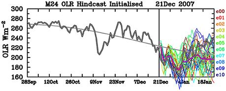
Figure 3. Example bias-corrected hindcast for start date 21 December 2007, showing ensemble mean (thick pink line) and all 33 ensemble members (3 members per rainbow color). Thick gray line shows the observed OLR from both before and after the model start date, and thinner gray line is the observed climatological seasonal cycle.

Hindcast Performance and Skill-Spread Relationship

Model OLR vs. Observed OLR

Model performance is evaluated for the bias-corrected multi-model ensemble mean OLR anomalies in comparison with the verifying observed OLR anomalies. Two metrics have been calculated; the correlation (shown later) and the root mean square (RMS) error for lead times from 1 to 35 days. These measures are calculated over all the hindcasts, and over various subsets. Figure 4 shows the RMS error for the ensemble mean from all hindcasts (upper panel) and for the summer monsoon months of December through March (DJFM; lower panel). Also shown are the RMS error for forecasts computed using climatology (i.e., a zero anomaly), the RMS error for persistence of the initial daily anomaly, and the hindcast “skill” computed as a percentage improvement of POAMA over climatology (using the same numerical scale as the error, i.e., from 0 to 40%).

FIGURE 4

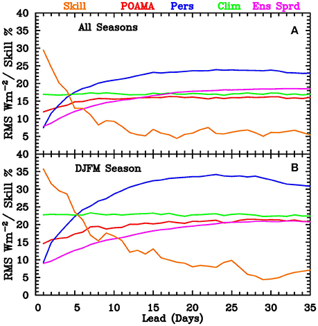
Figure 4. Root-mean-square (RMS) error of area-averaged OLR (in W m⁻², on a scale from 0 to 40 W m⁻²) for POAMA ensemble-mean hindcasts (red curve), reference forecasts using a forecast of zero anomaly (i.e., climatology; green), and persistence of the initial daily anomaly (blue). Also shown is the ensemble spread (magenta) in W m⁻², and skill score as a percentage improvement of POAMA over climatology (orange) on a scale from 0 to 40%. (A) Is for all seasons, and (B) for summer monsoon (DJFM) season only.

The RMS error of POAMA is smaller than that of both persistence and climatology for the range 2–35 days for both the all season and the summer monsoon (i.e., DJFM) season. Although the POAMA hindcast RMS error is greater in DJFM, the hindcasts are more skilful relative to climatology during this season, with a percentage improvement of about 36% at a lead of 1 day compared to 30% for the all-seasons case, and a percentage improvement of about 16% compared to 9% at a lead of 10 days. We contend that these percentage improvements represent a useful level of skill.

The spread (pink lines in Figure 4) for the all-season case is less than the model RMS error for days 1 to 12, i.e., indicating that the ensemble is under-spread. Between days 12 and 16 the spread is very close to the RMS error for both the model forecasts and climatological forecasts. Beyond day 16 the spread of the ensemble exceeds the RMS error of a climatological forecast, which implies that the POAMA forecasts have slightly greater variance than observed. For the summer months only, the ensemble appears to be under-spread for lead times up to about 20 days, and the spread stays below the RMS error of a climatological forecast for all leads.

Impact of MJO on Forecast Skill

As noted in the introduction, some, but not all, seasons show a strong relationship between the OLR over northern Australia and the phase of the MJO. It has also been previously shown that prediction of the RMM index of the MJO is somewhat more skilful when the MJO is strong at the initial time (Rashid et al., 2011). It therefore seems a reasonable hypothesis that the prediction of OLR over northern Australia should be more skilful when the MJO is strong in the initial conditions. We test this hypothesis by examining the impact of the MJO on the forecast skill when stratifying the hindcasts according to the presence or absence of a strong MJO signal (Figure 5A), and also by the phase of the MJO (Figure 5B) at the initial time. However, there is no evident impact of the amplitude or phase of the MJO on the hindcast RMS error. For the correlation skill (not shown), there appears a weak increase in correlation between days 2 and 9 for hindcasts initialized with a strong MJO, but it is not statistically significant. Thus we cannot confirm our hypothesis above. This appears consistent with the result of Marshall et al. (2011) who found that although POAMA was able to correctly simulate and predict the relationship between the MJO and rainfall (i.e., convection) over most of the tropical Indo-Pacific, it was not able to do this over the Maritime Continent and northern Australia, indicating that there is still room for improvement in these extended-range forecasts for northern Australia.

FIGURE 5

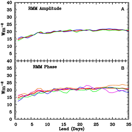
Figure 5. RMS errors of all POAMA hindcasts (A) stratified by RMM amplitude, blue for RMM > 1.3, green RMM ≤ 1.3, and red for all cases, and (B) stratified by RMM phase, with red for all cases, blue for phases 1 and 8, green for phases 2 and 3, magenta for phases 4 and 5, and orange for phases 6 and 7.

Ensemble Spread vs. Observed Uncertainty and Error

The relationship between the spread and the underlying observed variability is further highlighted by the rank histogram or “Talagrand diagram” (Talagrand et al., 1997; Hamill, 2001), shown in Figure 6 using all hindcasts. This histogram is constructed by counting where the verifying observation lies amongst all the ensemble members for each hindcast. Ideally the distribution should be flat, which occurs when the ensemble spread matches the observed variability, whereas a U-shaped distribution indicates insufficient spread with many verifying observations falling near the extremes or outside the range of the ensemble members, and a domed distribution indicates too much ensemble spread. All three types of distributions can be seen in Figure 6, which shows too little spread at 3 days lead, too much spread at 20 days lead, and about the right level of spread at 10 days lead. This result is consistent with Figure 4A which suggested that ensemble spread was insufficient at short leads (up to ~12 days) and over spread beyond about 16 days. The lack of ensemble spread at short lead times is exacerbated by the use of the same initial conditions for each of the three model configurations. This shows up in Figure 6 in the strong peak found at every third bin, due to the very small separation between the three ensemble members with identical initial conditions. As discussed by Hudson et al. (2013), this clearly signifies the need for using different initial conditions for each of the three model configurations.

FIGURE 6

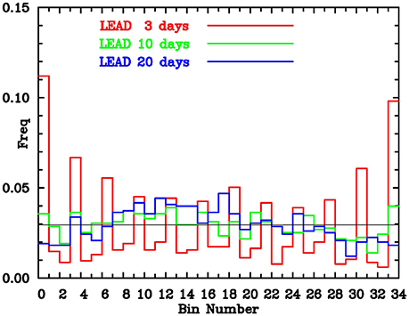
Figure 6. Rank histogram for hindcasts at 3-day (red), 10-day (green), and 20-day (blue) lead for all hindcasts. Thin black line is expected distribution assuming hindcasts fully represent observed uncertainty.

Binning the individual forecasts based on ensemble spread shows a generally positive relationship between spread and error (Figure 7). The spread-error correlations are 0.55 for the 3-day lead, 0.57 for the 10-day lead, and 0.90 for the 20-day lead. These correlations are more encouraging of a positive relationship between spread and error than others that have been listed in the literature (as reviewed by Grimit and Mass, 2007), especially for the 20-day lead. Therefore, especially for the 20-day lead, greater certainty can be given to forecasts with smaller spread.

FIGURE 7

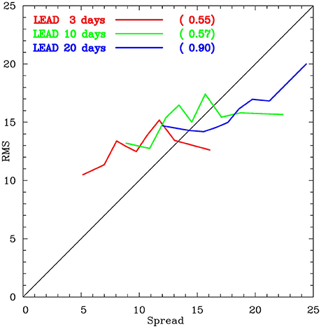
Figure 7. Spread vs. RMS error for hindcasts at a lead of 3 days (red) 10 days (green) and 20 days (blue). Binning of the hindcasts is based on the ensemble spread, using 9 bins containing 128 hindcasts each. Numbers in brackets are correlation between spread and RMS error for each lead time.

Real-Time Forecasts

Real-time forecasts have been performed once a week since August 2011 and twice a week since February 2013, and run out to at least 120 days. For most forecasts, the start date will not coincide with the dates for which hindcast climatologies are available. There are a number of possible strategies to obtain climatological values for any arbitrary start date. These include simply using the nearest available climatology or linearly interpolating between the two closest dates. The approach adopted here is to fit a smoothed annual cycle to each lead time, similar to the annual cycles for the observed and initialized data, and then obtain a climatological value for any start date and lead time by interpolation from this smoothed annual cycle. Smoothed annual cycles for lead times of day 1 (blue) and day 20 (green) are shown in Figure 2.

Real-time anomalies are then calculated in a similar manner to that used for the hindcasts. The consistency of the forecasts over a run of forecasts is demonstrated in Figure 8, which shows the ensemble mean of a sequence of 11 forecasts initialized between 04 Feb 2013 and 11 Mar 2013. This example shows a general agreement between one start time and the next, although with a notable exception to this for forecasts initialized before 1st March vs. those initialized after 1st March, showing that the model had a “change of heart” at that time. Comparison with the observed OLR anomalies shows that the forecast of positive OLR anomalies for 12–25 March by those forecasts initialized after 1st March, indicating suppressed convection, verified well. Overall, verification of all the available real-time forecasts (Figure 9) shows that the hindcast skill is generally maintained by independent forecasts. The limited real-time POAMA forecasts have lower RMS errors than persistence beyond the first day of the forecast, which is better than was the case for the hindcasts (Figure 4), which took 2–3 days to beat persistence. However, compared to climatological forecasts, the POAMA real-time forecasts lose skill more swiftly than the hindcasts, with the POAMA RMS error slightly exceeding that of climatology at lead times greater than about 15 days. We cannot think of a difference in the model prediction system between the hindcasts and real-time forecasts that could explain these skill differences (e.g., the model physics and initialisation remain the same), so we assume that the skill differences are a result of the rather short period (<5 years) of real-time data, and the associated statistical uncertainty this causes.

FIGURE 8

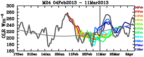
Figure 8. Real-time forecasts (area-averaged ensemble mean OLR) for all start dates from 4 February to 11 March 2013. Thick gray line shows the observed OLR from both before and after the model start dates, and thinner gray line is the observed climatological seasonal cycle.

FIGURE 9

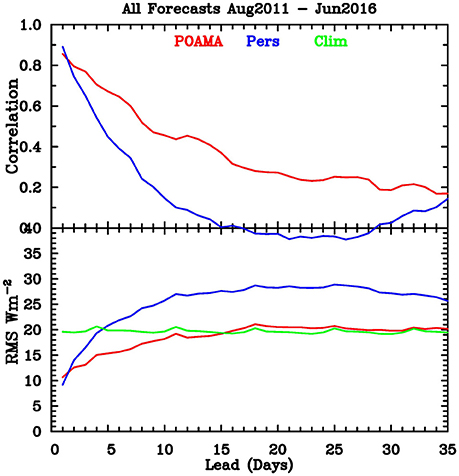
Figure 9. Verification of all available POAMA forecasts from August 2011 to June 2016 (red curves) compared with persistence (blue curves) and climatological forecasts (green curve) for the same period.

Conclusions

We examine the ability of the latest version of the POAMA system (POAMA-2M) to simulate the seasonal cycle of OLR over the north Australian monsoon region, and to predict its variability on timescales out to 35 days. After the period of initial shock is over (i.e., after the first few days), the model's seasonal cycle shows that it does not have enough convection during the wet season and consequently has smaller amplitude than observed. After correcting for this bias, model hindcasts show skill, over persistence and climatological forecasts, at lead times beyond 2 days. These hindcasts show that the model has greater skill during the summer monsoon season from December to March, but this skill is largely independent of the state of the MJO. Examination of the spread of hindcasts suggests that the model has insufficient spread at short lead times (<12 days), and slightly too much spread at longer lead times (>16 days). Real-time forecasts are constructed in a similar manner to the hindcasts, with the required bias correction obtained by interpolating the model seasonal cycle to give values at each real-time forecast start time. Verification of all available forecasts from August 2011 through to June 2016 suggests that the hindcast skill relative to persistence and climatology is mostly maintained in completely independent forecasts.

Author Contributions

WD and MW jointly designed the research, interpreted the results, and wrote the paper. WD analyzed the prediction system output and made Figures 2–9. MW made Figure 1, undertook the milestone reporting to funding bodies and managers, formatted the manuscript, and submitted the manuscript.

Funding

This work was partially supported during 2011–13 by the Northern Australia/Monsoon Prediction project of the Managing Climate Variability Program managed by the Grains Research and Development Corporation.

Conflict of Interest Statement

The authors declare that the research was conducted in the absence of any commercial or financial relationships that could be construed as a potential conflict of interest.

The reviewer SW and the handling Editor declared their shared affiliation, and the handling Editor states that the process nevertheless met the standards of a fair and objective review.

Acknowledgments

We thank the POAMA and related teams for their dedication to producing and maintaining POAMA, and for supporting its products. In particular, we thank Griffith Young for the POAMA web pages and computing support. Greg Browning and Andrew Marshall kindly provided internal reviews.

References

Grimit, E. P., and Mass, C. F. (2007). Measuring the ensemble spread–error relationship with a probabilistic approach: stochastic ensemble results. Mon. Weather Rev. 135, 203–221. doi: 10.1175/MWR3262.1

CrossRef Full Text | Google Scholar

Hamill, T. M. (2001). Interpretation of rank histograms for verifying ensemble forecasts. Mon. Weather Rev. 129, 550–560. doi: 10.1175/1520-0493(2001)129<0550:IORHFV>2.0.CO;2

CrossRef Full Text | Google Scholar

Hudson, D., Alves, O., Hendon, H. H., and Wang, G. (2011). The impact of atmospheric initialisation on seasonal prediction of tropical Pacific SST. Clim. Dyn. 36, 1155–1171. doi: 10.1007/s00382-010-0763-9

CrossRef Full Text | Google Scholar

Hudson, D., Marshall, A. G., Yin, Y. H., Alves, O., and Hendon, H. H. (2013). Improving intraseasonal prediction with a new ensemble generation strategy. Mon. Weather Rev. 141, 4429–4449. doi: 10.1175/MWR-D-13-00059.1

CrossRef Full Text | Google Scholar

Liebmann, B., and Smith, C. A. (1996). Description of a complete (interpolated) outgoing longwave radiation dataset. Bull. Am. Met. Soc. 77, 1275–1277.

Google Scholar

Marshall, A. G., and Hendon, H. H. (2015). Subseasonal prediction of Australian summer monsoon anomalies. Geophys. Res. Lett. 42, 10913–10919. doi: 10.1002/2015GL067086

CrossRef Full Text | Google Scholar

Marshall, A. G., Hudson, D., Hendon, H. H., Pook, M. J., Alves, O., and Wheeler, M. C. (2014a). Simulation and prediction of blocking in the Australian region and its influence on intra-seasonal rainfall in POAMA-2. Clim. Dyn. 42, 3271–3288. doi: 10.1007/s00382-013-1974-7

CrossRef Full Text | Google Scholar

Marshall, A. G., Hudson, D., Wheeler, M. C., Alves, O., Hendon, H. H., Pook, M. J., et al. (2014b). Intra-seasonal drivers of extreme heat over Australia in observations and POAMA-2. Clim. Dyn. 43, 1915–1937. doi: 10.1007/s00382-013-2016-1

CrossRef Full Text | Google Scholar

Marshall, A. G., Hudson, D., Wheeler, M. C., Hendon, H. H., and Alves, O. (2011). Assessing the simulation and prediction of rainfall associated with the MJO in the POAMA seasonal forecast system. Clim. Dyn. 37, 2129–2141. doi: 10.1007/s00382-010-0948-2

CrossRef Full Text | Google Scholar

Marshall, A. G., Hudson, D., Wheeler, M. C., Hendon, H. H., and Alves, O. (2012). Simulation and prediction of the Southern Annular Mode and its influence on Australian intra-seasonal climate in POAMA. Clim. Dyn. 38, 2483–2502. doi: 10.1007/s00382-011-1140-z

CrossRef Full Text | Google Scholar

Rashid, H. A., Hendon, H. H., Wheeler, M. C., and Alves, O. (2011). Prediction of the Madden-Julian oscillation with the POAMA dynamical prediction system. Clim. Dyn. 36, 649–661. doi: 10.1007/s00382-010-0754-x

CrossRef Full Text | Google Scholar

Stockdale, T. N. (1997). Coupled ocean–atmosphere forecasts in the presence of climate drift. Mon. Weather Rev. 125, 809–818. doi: 10.1175/1520-0493(1997)125<0809:COAFIT>2.0.CO;2

CrossRef Full Text | Google Scholar

Talagrand, O., Vautard, R., and Strauss, B. (1997). “Evaluation of probabilistic prediction systems,” in Proceedings, ECMWF Workshop on Predictability. Reading: ECMWF, 1–25.

Wheeler, M. C. (2008). Seasonal climate summary southern hemisphere (summer 2007-08): mature La Nina, an active MJO, strongly positive SAM, and highly anomalous sea-ice. Aust. Meteorol. Mag. 57, 379–393.

Google Scholar

Wheeler, M. C., and Hendon, H. H. (2004). An all-season real-time multivariate MJO index: development of an index for monitoring and prediction. Mon. Weather Rev. 132, 1917–1932. doi: 10.1175/1520-0493(2004)132<1917:AARMMI>2.0.CO;2

CrossRef Full Text | Google Scholar

Wheeler, M. C., and McBride, J. L. (2011). “Australasian monsoon,” in Intraseasonal Variability in the Atmosphere-Ocean Climate System, 2nd Edn, eds W. K. M. Lau and D. E. Waliser (Berlin: Springer), 147–198.

Google Scholar

Zhu, H., Wheeler, M. C., Sobel, A. H., and Hudson, D. (2014). Seamless precipitation prediction skill in the tropics and extratropics from a global model. Mon. Weather Rev. 142, 1556–1569. doi: 10.1175/MWR-D-13-00222.1

CrossRef Full Text | Google Scholar