Surface Energy Balance Closure and Turbulent Flux Parameterization on a Mid-Latitude Mountain Glacier, Purcell Mountains, Canada

Introduction

The observed large-scale retreat of mountain glaciers is a primary indicator of current climate change, and the loss of mass from these systems may have significant future impacts on sea level rise, freshwater supply, hydroelectric power production, and aquatic habitats (IPCC, 2013). In Western Canada, glaciers are projected to lose 70 ± 10% of their volume by the end of this century, relative to 2005 (Clarke et al., 2015). Enhanced understanding of the processes taking place at the ice—atmosphere boundary, and the role of these processes in glacier melt, is vital for improving both long-term predictions of glacier mass balance, and short-term modeling of meltwater runoff. Utilizing a surface energy balance (SEB) model can reduce the reliance on local, empirically-derived melt relationships used in other modeling techniques (e.g., temperature index models) which can vary spatially and temporally, requiring calibration for each glacier, and limiting transferability. However, in situ measurements of the complete SEB are rare on glacier surfaces, necessitating the use of parameterization methods for one or more of the energy fluxes in the majority of studies. Following radiation, the turbulent fluxes of sensible and latent heat (Q_H and Q_L) are generally assumed to be the next largest contributors to surface melt energy, and in some cases, can dominate the budget on daily and seasonal timescales (e.g., Anderson et al., 2010). Direct observations of Q_H and Q_L are scarce on glacier surfaces, however. The parameterization methods commonly used to estimate these fluxes contain substantial uncertainties, with a lack of observed data to evaluate their performance.

A small number of glacier SEB studies have attempted to measure Q_H and Q_L directly using the eddy covariance (EC) technique (e.g., Munro, 1989; Cullen et al., 2007; Litt et al., 2015). The installation and power requirements of this technique, along with difficulties in fulfilling the necessary measurement assumptions (outlined in Section SEB Background) have limited the use of EC systems in glacial settings, and the length of useable datasets where measurements exist. As a result of these challenges, Q_H and Q_L have been parameterized in the vast majority of SEB studies, utilizing the bulk aerodynamic method (e.g., Hay and Fitzharris, 1988; Arnold et al., 2006; Anderson et al., 2010; Van As, 2011). One of the largest sources of uncertainty in using the bulk method arises from the selection of appropriate values for the roughness lengths of momentum (z_0v), temperature (z_0t), and water vapor (z_0q). Where observations of z_0v exist, differences of several orders of magnitude across a range of glacier surfaces have been identified (Brock et al., 2006). However, the majority of SEB studies do not have access to site-specific z_0v observations, and instead select values from existing studies on surfaces deemed to have similar characteristics to the glacier of interest (Mölg and Hardy, 2004; Gillet and Cullen, 2011; Giesen et al., 2014). z_0v is often assumed to remain constant with time, with some studies implementing different values for when the surface is snow or ice covered. A range of methods have been used for expressing the relationship between z_0v, and the scalar roughness values of z_0t and z_0q, including the assumption that the three roughness lengths are equal (e.g., Gillet and Cullen, 2011; Dadic et al., 2013). It would be expected, however, that z_0v be different, and potentially considerably larger than z_0t and z_0q, as the surface properties governing momentum and scalar transport (form drag and molecular diffusion, respectively) have different spatial scales (Beljaars and Holtslag, 1991). To account for this, some studies implement a ratio of z_0v/10 or z_0v/100 to express z_0t and z_0q (e.g., Hock and Holmgren, 2005). The surface renewal model proposed by Andreas (1987) for determining z_0t and z_0q over snow and sea ice (from a given z_0v value) is also commonly implemented in glaciology studies (e.g., Giesen et al., 2014).

The bulk method assumes a logarithmic wind speed profile with height; an assumption only valid in statically neutral surface layers (Stull, 1988). Some studies attempt to account for the effects of varying atmospheric stability by introducing corrections, such as those based on the bulk Richardson number Ri_b (e.g., Sicart et al., 2005), and the Monin-Obukhov length L (e.g., Van den Broeke et al., 2005). These empirically-derived stability functions were developed over horizontal, homogeneous terrain, often cropland or forestry, and uncertainty remains regarding the validity of these corrections over inhomogeneous, sloped glacier surfaces. In particular, the assumptions of the Monin-Obukhov similarity theory (e.g., constant flux layer, stationarity, negligible advection) may not hold during strongly stable atmospheric conditions over glaciers, when the development of density driven, downslope “katabatic” winds is common. Wind speed profiles with a maximum close to the surface can exist in these conditions, resulting in steep eddy diffusivity gradients, and a suppressed constant flux layer, decoupling the fluxes calculated at measurement height from the true surface values (Denby and Greuell, 2000; Grisogono and Oerlemans, 2001).

In summary, glacier SEB models generally rely on some form of parameterization to close the energy budget, due to an absence of observed values for fluxes of interest. This lack of direct measurement, however, particularly in the case of the turbulent heat fluxes, has limited the opportunities to evaluate the employed parameterization techniques, and to better understand the underlying atmospheric—glacial processes. To address these issues, the initial goal of this study is to obtain an accurate, season-long dataset of the complete SEB on a sloped glacier surface. Direct observations of each flux, including those of the turbulent heat fluxes obtained through EC methods, will be used to drive a point SEB ablation model, and to assess the relative contribution of each flux to melt energy on the study glacier i.e., the energy partitioning. The performance of the SEB model in simulating observed surface ablation will indicate the ability of the employed measurement and data processing techniques to successfully capture glacier SEB. With confidence achieved in the reliability of the observed data, the performance of commonly used bulk method parameterizations of the turbulent heat fluxes will be evaluated through comparison with EC observations. This will include a comparison of commonly assumed roughness length schemes with EC-derived values for the study site. The overall impact of the choice of turbulent flux parameterization on SEB model performance will then be assessed.

SEB Background

SEB models attempt to account for all the energy terms contributing to mass changes at the glacier surface; a goal referred to as “closing” the energy budget. These terms include the four radiation fluxes of incoming shortwave (S_i), reflected shortwave (S_r), incoming longwave (L_i), and outgoing longwave (L_o), the four often combined into the net radiation flux (Q_N), the turbulent fluxes of sensible and latent heat, the heat flux due to rain (Q_R), and the ground heat flux due to temperature gradients in the ice (Q_G). SEB models utilize measurements or estimates of the above fluxes, in order to determine the energy available for melting, Q_M (Cullen et al., 2007; Giesen et al., 2014):

$\begin{array}{ll}{S}_i+S_r+L_i+L_o+Q_H+Q_L+Q_R+Q_G=Q_M& (1)\end{array}$

with Q_R and Q_G often deemed negligible in studies on mid-latitude glaciers (Sicart et al., 2005; Andreassen et al., 2008; Gillet and Cullen, 2011). For the direct measurement of Q_H and Q_L, the EC technique correlates high frequency measurements of the turbulent components of vertical wind speed (w) with those of potential temperature (θ) and specific humidity (q), to determine the magnitude and direction of the fluxes:

$\begin{array}{ll}{Q}_H=\overline{w^{\prime }{\theta }^{\prime }}{\rho }_a{c}_p,& (2)\end{array}$

$\begin{array}{ll}{Q}_L=\overline{w^{\prime }{q}^{\prime }}{\rho }_a{L}_v,& (3)\end{array}$

where the prime denotes the turbulent component, the overbar denotes a mean value (generally averaged over 30 min), ρ_a is air density (calculated from observed atmospheric pressure), c_p is the specific heat capacity of air (1,005 J kg⁻¹ K⁻¹), and L_v is the latent heat of vaporization (2.514 MJ kg⁻¹), substituted with the latent heat of sublimation (L_s = 2.848 MJ kg⁻¹) if surface temperature is below 0°C. A range of assumptions are generally required to be satisfied in order for EC measurements to be considered valid (Burba, 2013), including: (i) observations are taken within the constant flux layer where fluxes are representative of the surface of interest; (ii) the footprint (upwind source area for the turbulence observed at the sensor) is homogeneous and representative of the study site; (iii) turbulence is fully developed and stationary with minimum flow divergence/convergence; and (iv) the sensor installation itself is not disrupting air flow (Lee et al., 2004; Aubinet et al., 2012).

For parameterizing Q_H and Q_L, the bulk aerodynamic method employs an integrated form of the gradient transport or “K-closure” theory equation for turbulent flux (Stull, 1988). The unknown terms in Equations (2) and (3) i.e., $\overline{w^{\prime }{\theta }^{\prime }}$ and $\overline{w^{\prime }{q}^{\prime }}$, are described using mean values of wind speed (u), and the finite differences in mean values of potential temperature and specific humidity between the surface (s), and a single measurement height (z):

$\begin{array}{ll}{Q}_H={\rho }_a{c}_p{C}_{\theta }\overline{u}({\overline{\theta }}_z-{\overline{\theta }}_s),& (4)\end{array}$

$\begin{array}{ll}{Q}_L={\rho }_a{L}_v{C}_q\overline{u}({\overline{q}}_z-{\overline{q}}_s).& (5)\end{array}$

The bulk transfer coefficient (C_θ/q) represents the eddy diffusivity for θ or q through the surface layer. It is derived from the logarithmic wind speed profile equation, and is a function of measurement height and the roughness length values for momentum (z_0v), temperature (z_0t), and water vapor (z_0q). As mentioned, a range of functions have been applied to C_θ/q to account for the effects of atmospheric stability on the turbulent transfer of momentum and scalars (detailed in Section Bulk Method Evaluation).

Data and Methods

Station Design

A customized automatic weather station (AWS) was developed for use in this project. The station housed a suite of meteorological sensors (Table 1), including a four component radiometer to measure each of the radiation fluxes, and a tipping bucket rain gauge to observe precipitation (and calculate Q_R). The temperature profile of the surface layer of ice was measured for the calculation of Q_G using two thermistor arrays drilled into an initial depth of 4 m, with thermistor spacing of 0.25 m in the upper 1 m, and 1 m in the lower 3 m. A sonic ranger was used to observe changes in surface height due to ablation or snowfall. To directly measure the turbulent heat fluxes, the EC method was employed. A combined sensor, comprising a sonic anemometer and an open path infrared gas analyser was selected for this campaign. With this design, the anemometer and analyser components instantaneously measure the same sample volume, minimizing temporal and spatial errors due to the physical separation of the sensors. The sampling frequency of the EC measurements was 20 Hz, with the values averaged over 30 min blocks when calculating the magnitude and direction of the turbulent fluxes.

TABLE 1

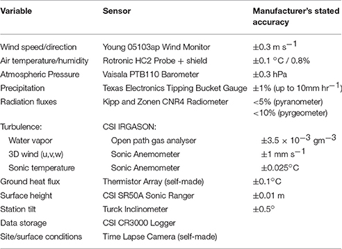
Table 1. Instrumentation used in this study.

In the atmospheric surface layer, significant gradients with height of temperature, humidity, and wind speed are typical. Therefore, it is important that meteorological sensors are maintained at a constant height above the surface if comparable measurements over time are required. The EC sensors are particularly sensitive to height changes, as increasing the height of the EC sensor may change the footprint from which the turbulence observed by the sensor is received (Burba, 2013). The sensor will also be at an increased risk of being positioned above the surface layer during strongly stable conditions, meaning that the sensor would no longer be observing eddies with characteristics of the glacier surface fluxes (Aubinet, 2008). To avoid these errors, the main meteorological sensors (including the EC system) were installed on a custom-built four-legged “quadpod,” which sits on the surface of the glacier (rather than being drilled in place), and lowers with the surface during the melt season (Figure 1). This ensured that the sensors maintained a constant height above the surface (wind monitor height z_u: 2.7 m, EC and temperature/humidity sensors height z: 2.0 m; radiometer height: 1.6 m). In order to monitor and correct for any tilting of the station that may occur over the season, an inclinometer was fitted to the quadpod to record its tilt angle in the x and y planes. The sonic ranger, along with the rain gauge, was mounted on a separate mast that was drilled into the ice, so that relative changes in glacier surface height could be measured. Observations were saved in 1 min averages (1 min totals for rainfall; 30 min samples for ice thermistors), while the eddy covariance data was stored in raw (20 Hz) format. A time lapse camera was also installed onsite, recording eight images per day of the surface and atmospheric conditions, and the general position and order of the AWS.

FIGURE 1

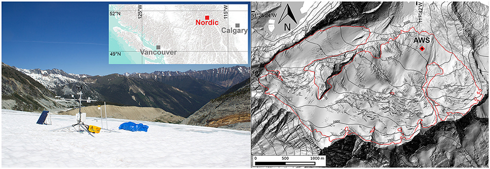
Figure 1. Installed AWS (as viewed by the time lapse camera), and its location on Nordic Glacier (red outline over LiDAR imagery) in the Purcell Mountains, BC, Canada, during the 2014 melt season.

Field Campaign

The described AWS was deployed during the summer of 2014 on Nordic Glacier (51°26′N, 117°42′W) in the Purcell Mountains in eastern British Columbia (BC), Canada. Nordic is a small (~5 km²), north-facing glacier, with an elevation range from 2,000 to 2,900 m a.s.l. (meters above sea level), approximately (Figure 1). The glacier is within the basin of the Columbia River; an important aquatic environment, and water source for irrigation and hydroelectric power production in BC, and the United States (Columbia Basin Trust, 2017). Previous studies within this basin indicate that glacier runoff may contribute up to a third of total streamflow during summer months (Jost et al., 2012). The AWS was installed in the ablation zone of the glacier (2,200 m a.s.l.) from July 11th to August 28th 2014, with the first and last days of measurements excluded from the study, to avoid contamination of the data due to installation activity. The study period therefore runs for 47 days from 00:00 on July 12th, day of year (DOY) 193, to 23:30 on August 27th (DOY 239). The station site was selected in the area with the lowest surface slope angle (8°), and with the most uniform upwind footprint, to help minimize the corrections required when processing the radiation and EC data. The station was orientated so that the radiometer was located on the south side of the structure, in order to avoid shadowing of the sensor. The main axis of the EC instrument was positioned to point upslope into the direction of the prevailing wind (downslope flow), to minimize flow distortion due to air flow through the station structure. The AWS performed reliably over the study period, with the quadpod remaining stable throughout (tilting < 2°), the power system maintaining an adequate supply, and the data from all sensors (including the camera) being consistently logged without any evident systematic errors. One of the main concerns prior to deployment, was the reliability of an unattended EC system in a harsh environment for an extended period of time. Calibration of the sensor before and after deployment showed negligible drift in its measurements over the season, while the signal strength of the gas analyser (excluding rain events) decreased from 99 to 97%, staying well above the manufacturer recommended quality cut off point of 70% (Campbell Scientific Inc., 2013).

AWS Data Treatment

Eddy Covariance Data

The EC data underwent a series of preprocessing steps prior to retrieving the 30 min turbulent fluxes of sensible and latent heat. Relative to the air flow on a glacier, the sonic anemometer cannot be leveled perfectly i.e., its vertical (z) axis will not be perpendicular to the mean flow. The vertical wind component (w) as measured by the sensor will thus be contaminated by contributions from the horizontal (u and v) components. To correct for this, the sonic anemometer data must undergo coordinate rotation. For the complex, sloping terrain of a mountain glacier, where the mean vertical wind (w) may be non-zero, the double rotation method may not be suitable, and therefore, a planar fit method has been implemented for this study (Wilczak et al., 2001). Long term measurements of u, v, and w are used to construct a hypothetical plane to which the w axis is set perpendicular. The features and slope of a glacier surface can change over a melt season, however, meaning this hypothetical plane may not be valid over an entire period. In this study, the planar fit calculations were performed in 1 week blocks (seven times in total), to account for the ongoing evolution of the surface. As the gas analyser component of the open path EC system measures the molar/mass density (g m⁻³) of water vapor in the sample space, variations in air density due to changes in temperature will cause fluctuations in the water vapor density measurements which are independent of changes in the turbulent fluxes. The widely used Webb-Pearman-Leuning correction (Webb et al., 1980) has been implemented to account for these fluctuations. Additional preprocessing steps were taken to correct for potential high and low frequency flux loss using methods following Ibrom et al. (2007) and Moncrieff et al. (2004), respectively.

The open path gas analyser can be susceptible to spurious readings during precipitation events due to the build-up of droplets or snowflakes on the sensor windows, leading to inaccurate Q_L observations. The EC Q_L values from periods with observed precipitation and the following 90 min (309 values; 13.7%) were therefore removed from the dataset (Figure 2B). This period length was selected based on testing of the sensor prior to deployment, which showed approximately a 90 min recovery period after rainfall for the windows to dry and the signal strength to normalize. Both fluxes were also subjected to a test of stationarity (Foken, 2008). Q_H and Q_L were found to be non-stationary for 15.4 and 24.5% of the observation period, respectively (Figures 2A,B). For assessing the performance of the bulk aerodynamic method, and for the calculation of roughness lengths, rain affected and non-stationary periods were excluded from the analysis. For the calculation of SEB and modeled ablation, rainfall and non-stationary gaps in the EC data were infilled using an optimized bulk method; the details of which are described in Section Roughness Lengths. While there is uncertainty regarding the validity of the bulk method during non-stationary conditions, it was selected as the best available approach in this study, and returned a more realistic range of flux values than the EC data during these conditions (Figures 2A,B).

FIGURE 2

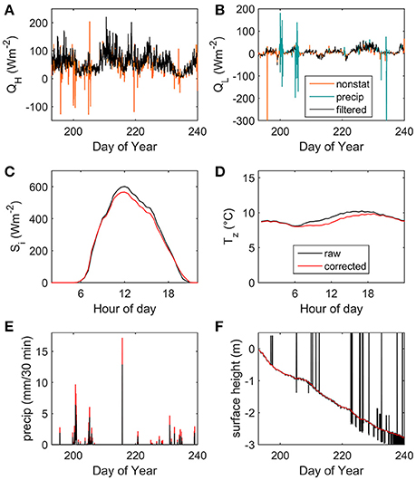
Figure 2. (A) Sensible and (B) latent heat fluxes with periods of non-stationary turbulence (orange) identified through the methods of Foken (2008), and periods of precipitation and the subsequent 90 min (teal), when the gas analyser windows may have been partially obscured. Also shown are the raw and corrected observation data for (C) the mean daily cycle (over 47 days) of incoming shortwave radiation, (D) the mean daily trend of near-surface air temperature, (E) 30 min precipitation, and (F) 30 min surface height.

Radiation Measurements

Observations of S_i are susceptible to errors at high solar zenith angles (Z_s) near sunrise and sunset, due to the poor cosine response of the sensor, particularly if the instrument is not level in the horizontal. In a number of studies (e.g., Andreassen et al., 2008), a 24 h running mean value for albedo (α) is calculated from the 30 min S_i and S_r data, and used to generate a new parameterized dataset for S_i. This correction method, however, does not account for sub-daily variations that can occur in α, due to snowfall, snow aging and removal, changing water content of the surface, and cloud amount. To allow for these variations, the S_i values in this study have only been corrected during periods when the sun is low in the sky. Based on the performance statistics provided by the radiometer manufacturer, a threshold value of Z_s > 65° was selected (Kipp and Zonen, 2009). A daily mean albedo value (α_d) is calculated from the observed S_i and S_r data when Z_s < 65°, and used to calculate S_i when Z_s > 65° (S_i = S_r/α_d). Observed S_i values are used for the remainder of the time.

When installed, the radiometer was leveled in the horizontal plane. The surface over which it is positioned, however, is sloped at an angle of 8°, and therefore, the intensity of the radiation exchange at this surface will be different from that recorded at the radiometer, and needs to be corrected for (Van den Broeke et al., 2004). As L_i, L_o, and S_r are assumed isotropic, only S_i is considered susceptible to this slope effect, and specifically, its direct component (D). As only global radiation (G) is measured by the radiometer (i.e., S_i = G), S_i is separated into its direct and diffuse (d) components following the methods of Hock and Holmgren (2005). The diffuse component is assumed to increase with cloudiness, which is estimated using the ratio (x) of S_i to the top of the atmosphere radiation (I_TOA):

$\begin{array}{ll}x=\frac{S_i}{I_{TOA}},& (6)\end{array}$

$\begin{array}{ll}\frac{d}{S_i}=\{\begin{array}{c}0.15forx\ge 0.8\\ 0.929+1.134x-5.111x^2+3.106x^{3}for0.15<x<0.8\\ 1forx\le 0.15\end{array}& (7)\end{array}$

Here, the empirical relationships derived in the above study (Equation 7) are assumed to be transferable to the Nordic site. A geometric correction is then applied to D, before it is recombined with the diffuse component to determine S_i at the surface (Jonsell et al., 2003):

$\begin{array}{ll}{D}_s=D\frac{cos\beta cos{Z}_s+sin\beta sin{Z}_{s}cos(\Omega -\theta )}{cos{Z}_s},& (8)\end{array}$

where D_s is the direct S_i component at the slope, Ω is the solar azimuth angle, β is the slope angle relative to the radiometer, and θ is the slope azimuth angle. β is updated every 30 min to account for any tilting of the radiometer from horizontal, as recorded by the inclinometer (< 2° over the study). The combined effect of the cosine response and slope corrections on the observed S_i (Figure 2C) resulted in a mean reduction of 4.1% in the energy of the flux over the season, and a maximum 30 min reduction of 7% (66.2 Wm⁻²).

The largest possible magnitude of L_o emitted by a melting snow/ice surface (at 273.15 K) is approximately 316 Wm⁻², and can be calculated using the Stefan-Boltzmann constant, σ (5.67 × 10⁻⁸ Wm⁻² K⁻⁴):

$\begin{array}{ll}{L}_o=\epsilon \sigma {T_s}^4+(1-\epsilon )L_i,& (9)\end{array}$

where ε is longwave emissivity (0.98), and T_s is the surface temperature (Park et al., 2010). This method accounts for the effect of emissivity and reflected L_i on the L_o value observed by the sensor. The observed L_o dataset was found to regularly exceed these calculated maximums (+10.1 Wm⁻² or +3%, on average). This may have been due in part to the sensor receiving additional longwave radiation emitted by the station structure when warmed above 0°C. To correct for this, observed L_o values in excess of this threshold were lowered to the calculated maximum. An independent surface temperature measurement would be a useful addition to the system in future deployments.

Air Temperature Correction

The air temperature and humidity probe was housed in a naturally ventilated radiation screen, rather than in a mechanically aspirated screen, due to power constraints. As a result, the data may suffer from errors due to radiative heating of the sensor during periods of strong solar radiation (WMO, 1983; Hock and Schroff, 2004; Obleitner, 2004; Fitzpatrick, 2007). To account for this, a correction was implemented using the sonic temperature from the sonic anemometer, which is assumed less susceptible to radiation error. The sonic temperature (T_sonic) was converted to air temperature (T_sa) using the method of Kaimal and Gaynor (1991):

$\begin{array}{ll}{T}_{sa}=\frac{T_{sonic}}{(1+0.32\frac{e}{p})},& (10)\end{array}$

where e is vapor pressure, and p is atmospheric pressure. T_sa and e were calculated iteratively to account for the initial uncorrected air temperature value used to calculate e. The values of T_sa were then compared with the air temperature observations from the sensor in the screen (T_z), during nighttime periods (no solar radiation) with wind speeds above 3 m s⁻¹ when the screen is well ventilated (Harrison, 2010), to obtain the mean bias between the sensors (−0.17°C). This bias was removed from T_sa to obtain T_{sa_unbiased}, which in turn was subtracted from T_z to calculate differences from measured air temperature (T = T_z − T_{sa_unbiased}). The variation of T with S_i was examined, and found to be well represented by a 2nd order polynomial ($T=-5.5x10^{-7}{S_i}^2+0.0017S_i-0.052$; r² = 0.76). This empirical fit was employed to estimate the correction required for radiation error in T_z for a given S_i magnitude, resulting in a mean temperature reduction of 0.3°C and a maximum reduction of 1.1°C (Figure 2D) for a 30 min average. Adding wind speed to this regression analysis was tested, but was found not to improve the goodness of fit.

Rainfall Undercatch

Studies on tipping bucket rain gauges have observed extensive underestimation of rainfall amounts (of up to 50%), primarily due to acceleration of airflow over the top of the gauge, with other error sources including splashing, and the finite time required for the buckets to reset in between tips during heavy rain (e.g., Devine and Mekis, 2008; Duchon and Biddle, 2010). An empirical correction was applied to the Nordic data to account for wind effects, following the work on a similar gauge by Mekonnen et al. (2015). The correction factor, w_r, accounts for the effects of wind speed at gauge height, u_g, and precipitation intensity, I_p (mm/h), on the observations:

$\begin{array}{ll}{w}_r=\frac{1}{1-exp\left[(0.011-0.062ln(I_p))u_g-0.776\right]},& (11)\end{array}$

where

$\begin{array}{ll}{u}_g=u\frac{ln\left(\frac{z_g}{z_{0v}}\right)}{ln\left(\frac{z_u}{z_{0v}}\right)},& (12)\end{array}$

and z_g is the height of the rain gauge, which is continuously updated from its initial installed height using the surface height data from the sonic ranger (as the gauge was mounted on a fixed mast rather than the quadpod). Using this correction, the undercatch for the Nordic precipitation data was estimated to be 40.4%, on average (Figure 2E).

Surface Height Measurements

Surface height datasets obtained from sonic rangers are characteristically noisy, and require processing prior to use. The raw data were first corrected for the effect of air temperature variation on the speed of sound, following manufacturer guidelines (Campbell Scientific Inc., 2014). A low pass filter was applied to remove a series of unrealistic spikes in surface height change with rates above 0.04 m min⁻¹, and to replace them with values from the previous minute. The surface height values were then passed through a 24 h moving average filter, chosen to optimize the retrieval of a smooth dataset that still displays sub-diurnal fluctuations (Figure 2F).

Rain Heat Flux

Q_R was calculated by first cross-examining the data obtained from the rain gauge with T_z, and determining whether the precipitation was rain or snow, based on a threshold near-surface air temperature (in this case, 1°C). The energy received from rain events in Wm⁻² was then calculated following Hay and Fitzharris (1988):

$\begin{array}{ll}{Q}_R={\rho }_w{c}_{w}R(T_r-T_s),& (13)\end{array}$

where ρ_w is the density of water (1,000 kg m⁻³), c_w is the specific heat capacity of water (4,180 J kg⁻¹ K⁻¹), R is the rainfall rate, and T_r is the rain temperature which is assumed to be in equilibrium with T_z, and T_s is surface temperature. Apart from one brief period of snowfall on July 24th (DOY 205), all precipitation events during the study were deemed to have been rainfall. The utilized threshold air temperature for the occurrence or absence of snowfall was verified by examining the albedo values and camera images from these periods.

Ground Heat Flux

Q_G is estimated from the ice thermistor data, using the methods outlined in Konzelmann and Braithwaite (1995). Half-hourly flux profiles of the upper layer of the glacier were constructed using the following equation:

$\begin{array}{ll}H(z_{ice})=-K\frac{\Delta T_i}{\Delta z_{ice}},& (14)\end{array}$

where H(z_ice) is the heat flux at the depth of each thermistor (start of season depths for z_ice = 0.25–4 m), K is the thermal conductivity of ice (2.1 W m⁻¹ K⁻¹), and ΔT_i and Δz_ice are the differences in ice temperature and depth between z_ice and the surface. The magnitude of Q_G at the surface for each 30 min period was then estimated by fitting a linear regression to the flux profile, and taking the regressed value for H(0). With no significant sub-daily trends in the observed data, and to allow for the slow response time of the ice thermistors, daily averages for Q_G were used in the SEB equation. The changing depths of the thermistors over the season (z_ice) were estimated from the initial depths of their installation and the surface height data from the sonic ranger. Data from thermistors that come within 0.5 m of the surface were excluded, to minimize the influence of radiative heating of the cables.

Error Analysis

Following the above processing and correction steps, the random error in the values for each of the eight fluxes was estimated. Standard error propagation methods were implemented to calculate the uncertainty in Q_R and Q_G from the sensor accuracies (Table 1) and uncertainties in the variables in Equations (13) and (14) (e.g., R, T_s, T_i, z_ice). For Q_R, the assumption made in Equation (13) that T_r is in equilibrium with T_z may not hold true where strong near-surface gradients in air temperature exist. Therefore, an assumed uncertainty of ±2°C was assigned to T_r for the error propagation calculations. The random error in the EC-observed turbulent fluxes due to sampling errors was estimated following the methods of Finkelstein and Sims (2001). Where Q_H and Q_L values have been replaced by bulk estimated fluxes due to periods of precipitation or non-stationary turbulence, error propagation has been applied to Equations (4) and (5). As stated in Section Eddy Covariance Data, there may be additional unquantified uncertainty here due to the application of the bulk method during non-stationary conditions. Uncertainty values for the shortwave and longwave radiation fluxes, as provided by the sensor manufacturer (Kipp and Zonen, 2009), are listed as being <5% and <10%, respectively, for daily totals. To refine these values for the measurements in this study, the uncertainty in the shortwave fluxes was estimated from the deviations of the raw S_i and S_o measurements from 0 Wm⁻² at night, and for the longwave fluxes from the deviations of the L_o measurements from the values expected for a melting surface (Litt et al., 2015). The smoothed surface height dataset also contains uncertainty due to the choice of length of moving average filter used (Section Surface Height Measurements). A range of time lengths were tested for the filter window (3–48 h), and the maximum and minimum height values for each period were used to determine the uncertainty range on the 24 h filtered data.

SEB Model

In the first stage of the model, the observed energy fluxes are converted into 30 min averages and summed to obtain averages of Q_M in Wm⁻² (Equation 1). The general convention in glacier SEB studies is that fluxes resulting in a gain in energy of the surface have a positive sign. The maximum temperature a snow/ice surface can be warmed to is 0°C. When the glacier surface is at this temperature, any positive energy available in the Q_M term is used by the model to generate melting (Hock, 2005):

$\begin{array}{ll}M=\frac{Q_M}{{\rho }_w{L}_f},& (15)\end{array}$

where M is the average melt per second (for a given 30 min average of Q_M) in m of water equivalent (m w.e. s⁻¹), and L_f is the latent heat of fusion (0.334 MJ kg⁻¹). The unit of m w.e. expresses the thickness of the layer melted (per m² of area) when the snow/ice is converted to water. The surface temperature of the glacier is estimated in the model using the observed (corrected) longwave radiation data (Equation 9). Sublimation (in m w.e. s⁻¹) is also accounted for in the model. A negative/positive value for Q_L (i.e., a loss/gain of latent heat energy) indicates mass loss/gain through sublimation/resublimation and can be accounted for as follows:

$\begin{array}{ll}sub/resub=\frac{|Q_L|}{{\rho }_w{L}_s},& (16)\end{array}$

where |Q_L| denotes the absolute value. The values for melt and sublimation, converted from averages to 30 min totals, are summed together to calculate surface ablation (a). The performance of the SEB model is evaluated by comparing the values it generates with the data observed by the sonic ranger. Modeled ablation is converted into surface height changes (z_gM) by multiplying the half hourly ablation totals by the ratio of the snow or ice density (ρ_s/i) to ρ_w:

$\begin{array}{ll}{z}_{gM}=a\frac{{\rho }_{s/i}}{{\rho }_w}.& (17)\end{array}$

A thin layer of packed snow covered the site surface for the first 3 days of observations, and a constant value of 400 kg m⁻³ was used for ρ_s. For the remaining period, the ice surface was assumed to have a constant density of 900 kg m⁻³ (Arnold et al., 2006; Gillet and Cullen, 2011; Van As, 2011). These surface height values can then be compared directly with the smoothed values from the sonic ranger. Accumulation due to snowfall and deposition is also added to the modeled surface height, so as to more accurately follow the observed values. During the single, brief period of snowfall (0.001 m w.e. approx.), a density of 80 kg m⁻³ was assumed for the fresh snow; a low density value to account for the thin and incomplete coverage of snowfall over the study site.

Bulk Method Evaluation

The performances of bulk method parameterizations of the turbulent heat fluxes (Equations 4 and 5) were evaluated through comparisons with the observed fluxes from the EC system. Three of the bulk transfer coefficient forms most commonly used in glacier studies have been tested here. The first form assumes neutral atmospheric stability (excludes a stability function), and a logarithmic wind speed profile (e.g., Conway and Cullen, 2013):

$\begin{array}{ll}{C}_{log}=\frac{k^2}{ln\left(\frac{z_u}{z_{0v}}\right)ln\left(\frac{z}{z_{0t/q}}\right)},& (18)\end{array}$

where k is the von Kármán constant (0.4). The second form includes a function for stability based on the bulk Richardson number, R_ib (Webb, 1970; Brock et al., 2010):

$\begin{array}{ll}{C}_{bR}=\frac{k^2}{ln\left(\frac{z_u}{z_{0v}}\right)ln\left(\frac{z}{z_{0t/q}}\right)}\varphi ,& (19)\end{array}$

where

$\begin{array}{ll}{R}_{ib}=\frac{g(T_z-T_s)z}{T_z{u}^2},& (20)\end{array}$

$\varphi ={(1-{5R}_{ib})}^2$ for stable conditions (positive R_ib), and $\varphi ={(1-{16R}_{ib})}^{0.75}$ for unstable conditions (negative R_ib), and g is acceleration due to gravity (9.81 ms⁻²). The third form uses stability functions based on the similarity theory of Monin and Obukhov (1954), and is arguably the most frequently used stability scheme in glacier SEB models (Arnold et al., 2006; Giesen et al., 2014):

$\begin{array}{ll}{C}_{MO}=\frac{k^2}{\left[ln\left(\frac{z_u}{z_{0v}}\right)-{\psi }_m\left(\frac{z_u}{L}\right)\right]\left[ln\left(\frac{z}{z_{0t/q}}\right)-{\psi }_h\left(\frac{z}{L}\right)\right]},& (21)\end{array}$

where ${\psi }_m\left(\frac{z_u}{L}\right)$ and ${\psi }_h\left(\frac{z}{L}\right)$ are the vertically integrated stability functions for momentum and heat, with the stability function for water vapor, ${\psi }_e\left(\frac{z}{L}\right)$, assumed equal to ${\psi }_h\left(\frac{z}{L}\right)$. L is the Obukhov length:

$\begin{array}{ll}L=\frac{{\rho }_a{c}_p{u_{*}}^3{T}_z}{kg{Q}_H},& (22)\end{array}$

where u_* is the friction velocity (a function of shear or the vertical flux of horizontal momentum). Conceptually, L can be thought of as the height above the surface where buoyant forces equal shear forces in the production of turbulence (Stull, 1988). As L contains Q_H, an iterative scheme is used when solving Equations (4) and (22), following Munro (1989). The parameter $\frac{z_u}{L}$ is used to determine stability conditions, with $\frac{z_u}{L}$ < 0 implying unstable, $\frac{z_u}{L}$ > 0 implying stable, and $\frac{z_u}{L}$ = 0 implying neutral. In this study, the functions proposed by Beljaars and Holtslag (1991) have been used in Equation (21) for stable conditions:

$\begin{array}{ll}-{\psi }_m\left(\frac{z_u}{L}\right)=\frac{a{z}_u}{L}+b\left(\frac{z_u}{L}-\frac{c}{d}\right)exp\left(-\frac{d{z}_u}{L}\right)+\frac{bc}{d},& (23)\end{array}$

$\begin{array}{l}-{\psi }_h\left(\frac{z}{L}\right)={\left(1+\frac{2az}{3L}\right)}^{1.5}+b\left(\frac{z}{L}-\frac{c}{d}\right)exp\left(-\frac{dz}{L}\right)\\ +\frac{bc}{d}-1,& (24)\end{array}$

with a = 1, b = 0.667, c = 5, and d = 0.35. For unstable conditions, the methods of Dyer (1974) have been implemented:

$\begin{array}{ll}{\psi }_m\left(\frac{z_u}{L}\right)=log\left[\left(\frac{1+y^2}{2}\right){\left(\frac{1+y}{2}\right)}^2\right]-2ta{n}^{-1}y+\frac{\pi }{2},& (25)\end{array}$

$\begin{array}{ll}{\psi }_h\left(\frac{z}{L}\right)=2log\left(\frac{1+y^2}{2}\right),& (26)\end{array}$

where $y={\left(1-16\frac{z_u}{L}\right)}^{\frac{1}{4}}$ for Equation (25), and $y={\left(1-16\frac{z}{L}\right)}^{\frac{1}{4}}$ for Equation (26).

Roughness Lengths

The roughness length values for the Nordic Glacier site were calculated directly from EC-observed data for wind speed, air temperature, specific humidity, friction velocity, Monin-Obukhov length, and the surface layer scales for temperature and specific humidity (u_ec, T_ec, q_ec, u_*ec, L_ec, θ_*ec, and q_*ec, respectively) (Conway and Cullen, 2013):

$\begin{array}{ll}{z}_{0v}=exp\left[-k\frac{u_{ec}}{u_{*ec}}-{\psi }_m\left(\frac{z}{L_{ec}}\right)\right]z,& (27)\end{array}$

$\begin{array}{ll}{z}_{0t}=exp\left[-k\frac{T_{ec}-T_s}{{\theta }_{*ec}}-{\psi }_h\left(\frac{z}{L_{ec}}\right)\right]z,& (28)\end{array}$

$\begin{array}{ll}{z}_{0q}=exp\left[-k\frac{q_{ec}-q_s}{q_{*ec}}-{\psi }_h\left(\frac{z}{L_{ec}}\right)\right]z.& (29)\end{array}$

q_s is determined from the surface vapor pressure (e_s) which is assumed to be at saturation at T_s (q_s = 0.622e_s/p). A series of filters were applied to the 30 min data to identify periods optimal for calculating accurate roughness length values, representative of conditions on the glacier, and with minimum scatter. Wind direction is an important filter, and data were used when the wind was blowing from within a 90° window around the main axis of the EC sensor (which pointed to 225°), to minimize flow distortion due to air flow through the station structure. Minimum values for wind speed (3 m s⁻¹) and u_*ec (0.1 m s⁻¹) were also implemented to avoid large errors in z_0v. As previously described, precipitation can affect the data observed from the gas analyser. Measurements of u_*ec also displayed spiking during rainfall, and so periods of precipitation were excluded from roughness length calculations. Sufficient near surface gradients in temperature and vapor pressure are necessary to determine z_0t and z_0q. Therefore, filters for minimum differences in measurement and surface height values of air temperature (>1°C) and vapor pressure (>66 Pa) were applied (Calanca, 2001; Conway and Cullen, 2013). The mean free path length for molecules at the average pressure and temperature at the station was calculated to be approximately 1 × 10⁻⁷ m, and this value was used as a minimum physically plausible value for scalar roughness lengths (Li et al., 2016). As was carried out during pre-processing of the EC fluxes, turbulence for each 30 min period had to pass a test of stationarity (Foken, 2008) to be used for roughness length calculation. Due to the uncertainty regarding how valid the applied stability functions are for a glacier surface, a filter to only use data from near-neutral stability conditions ($-0.1<\frac{z}{L_{ec}}<0.2$), when these functions are negligible, has been applied (Smeets and van den Broeke, 2008; Conway and Cullen, 2013).

In addition to implementing the EC-derived roughness values calculated above, the bulk transfer coefficients were also evaluated using a number of the most commonly used “assumed” roughness length schemes from previous glacier studies, where site-specific measurements of roughness length are generally unavailable. Two sets of values for z_0t and z_0q were estimated by assuming both an equal and a 1/100 relation to z_0v, where z_0v is assumed to be 10⁻³ m for ice, and 10⁻⁴ m for snow (Mölg and Hardy, 2004; Hock and Holmgren, 2005). A third set of values for z_0t and z_0q was calculated using these assumed z_0v values and the surface renewal theory methods outlined by Andreas (1987), where the ratio of the scalar (z_0s) and momentum roughness lengths are expressed as a function of the roughness Reynolds number R_*:

$\begin{array}{ll}{R}_{*}=\frac{u_{*}{z}_{0v}}{\nu },& (30)\end{array}$

$\begin{array}{ll}ln\left(z_{0s}/z_{0v}\right)=b_0+b_{1}ln\left(R_{*}\right)+b_2{ln\left(R_{*}\right)}^2,& (31)\end{array}$

where ν is the kinematic viscosity of air (1.5 × 10⁻⁵ m² s⁻¹). The values of the empirical coefficients (b₀, b₁, and b₂) change for smooth (R_* ≤ 0.135), transitional (0.135 < R_* < 2.5), and rough (R_* ≥ 2.5) flow regimes. For infilling the gaps in the EC-observed flux data due to precipitation and non-stationary turbulence (Section Eddy Covariance Data), an additional set of effective roughness length values were also calculated, which were tuned to return the observed turbulent flux values when implemented with C_log. Daily averages of these roughness values were used in Equation (18) to estimate the missing flux data.

Results

Meteorological and Flux Observations

The meteorological conditions remained mild throughout the study period (Figure 3), with a mean T_z of 8.9°C and consistently positive air temperatures (max: 16.1°C; min: 0.6°C). Cloud coverage was generally low, as verified by camera imagery, resulting in high net shortwave radiation fluxes over the season (mean: 130.6 Wm⁻²) and low net longwave values (mean: −9.2 Wm⁻²). The surface temperature T_s, was estimated to be at melting point for >99% of the study period, with the temperature below 0°C for a total of 5 h (min: −0.3°C). Precipitation was confined to three frontal systems and sporadic convective showers (total: 293.7 mm), with a trace amount of snowfall on July 24th (DOY 205). The mean Q_R value was 1.7 Wm⁻² over the entire period, with a maximum 30 min average of 339.2 Wm⁻² during an individual event with a 34 mm/h rainfall rate (DOY 215). Winds were generally light and steady, with a mean of 3.5 m s⁻¹ and a maximum 30 min average of 7.2 m s⁻¹. The mean wind direction was 204°, which accords with the downslope air flow on the glacier. The wind remained within ±45° of this direction for 91% of the observation period, and within ±90°For 97% of the period, with no evident diurnal cycle. The positioning of the EC sensor within the prevaling wind window (main axis: 225°) ensured that, for the vast majority of observations, air flow was sampled by the EC system prior to being distorted by the station. Q_H remained positive for the entire observation period, with a mean value of 59.4 Wm⁻². Q_L fluctuated about zero, with a mean value of 9.0 Wm⁻². The ice thermistors recorded a small temperature gradient in the near-surface ice layer (~0.9°C over 4 m). As the thermistor cables gradually melted out over the season, the depth range of ice temperature measurements reduced. From the available data, little change is observed in the temperature profile over time, with a slight warming trend commencing a few days after the removal of the snow layer (DOY 196). With such a small temperature gradient, Q_G remained small, with a mean value of -0.7 Wm⁻².

FIGURE 3

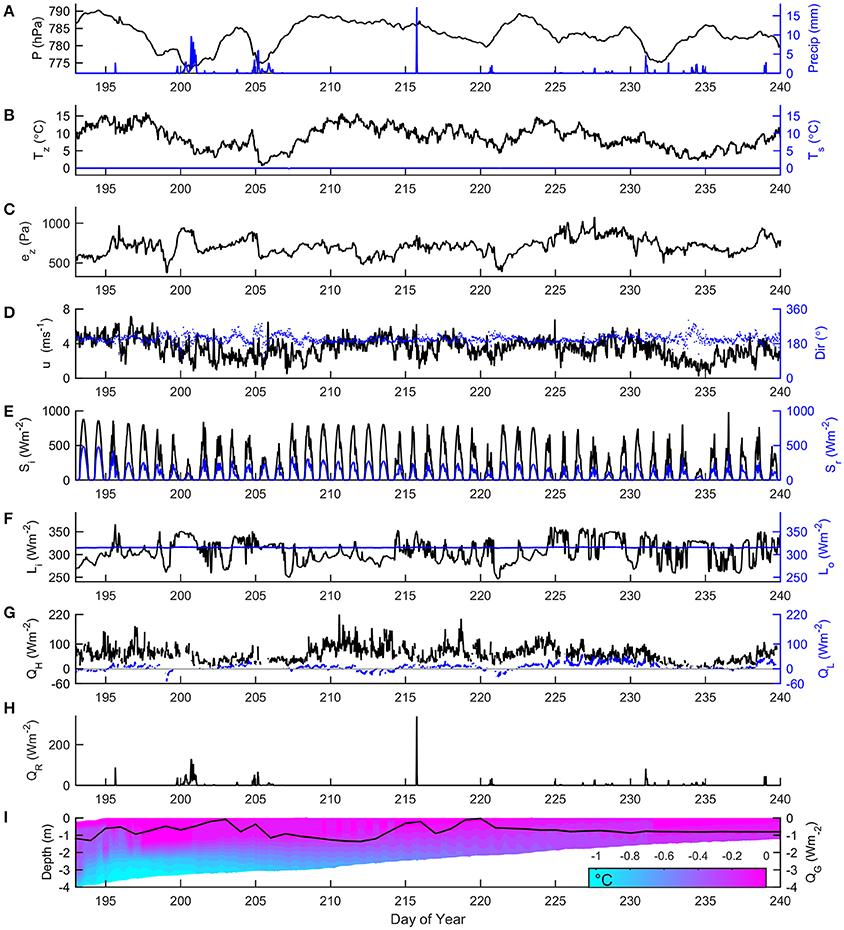
Figure 3. Thirty minute meteorological data and surface energy fluxes for July 12th–August 28th (DOY 193–240) 2014 on Nordic Glacier; (A) pressure and precipitation, (B) 2 m air and surface temperature, (C) 2 m vapor pressure, (D) wind speed and direction, (E) incoming and reflected shortwave, (F) incoming and outgoing longwave, (G) sensible and latent heat fluxes, (H) rain heat flux, and (I) ice temperature profile and ground heat flux.

Error analysis performed on each of the observed fluxes returned daily average error values substantially smaller than the fluxes themselves (Table 2). The obtained mean uncertainties for shortwave and longwave fluxes of 1.9 and 3.3% are in line with those estimated in previous studies using similar sensors (Van den Broeke et al., 2004). It should be noted that there remains unquantified uncertainty in S_i and Q_R due to the previously described empirical corrections applied to the data. The combined effect of the errors in each flux were propagated to obtain the error in Q_M (mean relative error: ±9.9%). The uncertainity in the surface height data due to the required smoothing was calculated to be ±0.001 m (±71.4%) and ±0.008 m (±13.8%) for mean 30 min and daily values, respectively.

TABLE 2

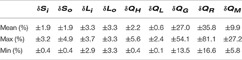
Table 2. Range of the daily average error values (% of mean fluxes) calculated for the eight observed fluxes and Q_M.

Ablation Modeling and Surface Energy Balance Partitioning

The ablation values obtained from the SEB model show good agreement with those recorded by the sonic ranger (Figure 4). Both modeled and observed data returned a net surface ablation of 2.74 m over the 47 days. Examining model performance in estimating 30 min changes in surface height, the model showed a correlation (r) of 0.75 with the ranger data, and a root-mean-square error (RMSE) of 0.001 m/30 min. On a daily time scale, model performance was considerably improved (r: 0.86; RMSE: 0.02 m/day). Net radiation (Q_N) was the largest contributor to the melt energy, providing 65.2% over the study period (Figure 5A), with the longwave fluxes effecting a net loss of energy from the surface (−7.6% of Q_N), as shown in Figure 5B. Q_H was the second largest contributor with 29.7%, followed by Q_L with 4.5%. Due to the low magnitude and frequency of negative Q_L fluxes, little sublimation was observed during the season (0.1% of total ablation), while total resublimation (during positive Q_L periods) was estimated at 0.014 m w.e. Providing just 0.9% of the total melt energy, Q_R was observed to be the smallest positive contributor over the season, while Q_G was found to be a small surface energy sink (−0.4%). The day with the greatest observed ablation (in terms of m w.e) was July 29th (DOY 210), with 0.1 m w.e. of loss. This corresponds with the day of maximum net energy received at the surface, with a mean flux value of 288.8 Wm⁻² observed (55% above the average daily value for the study).

FIGURE 4

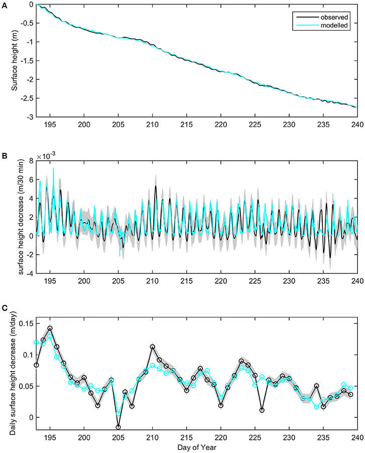
Figure 4. Observed (black) and modeled (cyan) surface height changes due to ablation/accumulation on Nordic Glacier, summer 2014; (A) surface height trend over the season, (B) 30 min rate of surface height change, and (C) daily rate of surface height change (midnight to midnight). The gray shading represents the uncertainty in the observed surface height values arising from the choice of moving average filter length when processing the sonic ranger data.

FIGURE 5

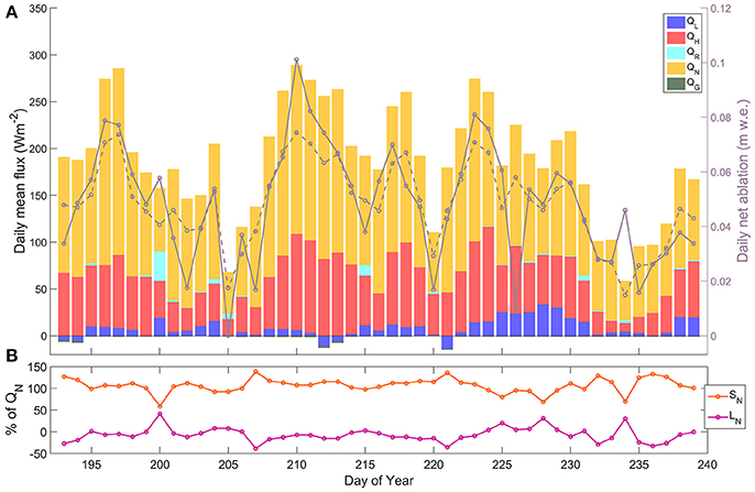
Figure 5. (A) Daily mean energy fluxes, and the daily net observed and modeled ablation (solid and dashed gray lines, respectively), and (B) percentage contribution of net shortwave and longwave radiation (S_N and L_N) to daily Q_N.

Roughness Length Values

As previously described (Equations 27–29), the EC data obtained on Nordic Glacier were used to calculate a dataset of site-specific roughness length values (ec_z). Atmospheric conditions were predominately stable over the glacier (89% of study, as determined by $\frac{z}{L_{ec}}$) with few periods of neutral stability. As a result, application of the stability filter (along with the other filters described in Section Roughness Lengths) returned 69, 56, and 11 30-min periods for z_0v, z_0t and z_0q, respectively, when the values were deemed representative of the study surface. The mean log values of the roughness lengths (± 1 standard deviation) for these periods were 10^{−2.3 ± 0.9} m, 10^{−4.6 ± 1.1} m, and 10^{−6.0 ± 0.8} m, respectively. In Figure 6, the ec_z values are compared with those estimated from the most commonly used roughness length schemes from existing glacier SEB studies: “equal” (z_0v = z_0t = z_0q); “1/100” (z_0v/100 = z_0t = z_0q); the Andreas (1987) surface renewal method for z_0t (mean: 10^−3.4 m) and z_0q (mean: 10^−3.2 m). For each of these three methods, z_0v is assumed to be 10⁻³ m for ice and 10⁻⁴ m for snow cover (as discussed in Section Roughness Lengths). Based on camera and albedo observations, the surface was assumed to transition from snow-covered to ice-covered after the first 4 days (DOY 197). Separating the EC-derived z_0v values into periods with a snow or ice surface produced mean values of 10^{−3.8 ± 1.7} m and 10^{−2.2 ± 0.7} m, respectively.

FIGURE 6

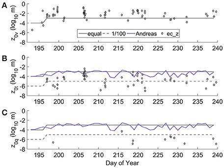
Figure 6. Thirty minute EC-derived roughness length values for (A) momentum, (B) temperature, and (C) water vapor, compared with commonly assumed roughness length schemes from the literature. For the assumed schemes, z_0v is 10⁻³ m for ice, and 10⁻⁴ m for snow (surface of the turbulence footprint area transitioned from snow to ice on DOY 197).

Bulk Method Evaluation

Three forms of the bulk transfer coefficient (Equations 18–26), and the previously discussed range of observed and assumed roughness length values, were implemented to obtain 12 sets of bulk-estimated turbulent heat fluxes (see Table 3 and Figure 7). Where the ec_z data were used, the means of the available roughness length values were implemented (separating z_0v for snow and ice). Evaluating the bulk estimates of the fluxes against the EC observations was only carried out for periods with ideal EC measurement conditions, namely those that passed the filters used when calculating the roughness lengths (Section Roughness Lengths), excluding the stability filter. Therefore, 691 and 380 periods (31 and 17% of study period) were useable for Q_H and Q_L comparisons, respectively. The flux values returned by each bulk method varied greatly depending on the paired roughness scheme. For the ec_z values, C_log and C_MO show significant correlation with the EC-observed fluxes, in particular, for Q_L (r = 0.89, p < 0.01). Weaker correlation exists between C_bR and the observed fluxes, particularly for Q_H, in addition to substantial underestimation of Q_H and Q_L (MBE: −29.1% and −25.5%). Conversely, C_log and C_MO, substantially overestimate both fluxes. For the range of assumed roughness schemes, C_log, when coupled with the 1/100 roughness scheme, produces flux values closest to those observed.

TABLE 3

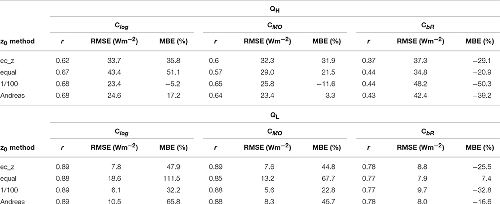
Table 3. Performance of the tested bulk methods in modeling the EC-observed turbulent fluxes of sensible and latent heat.

FIGURE 7

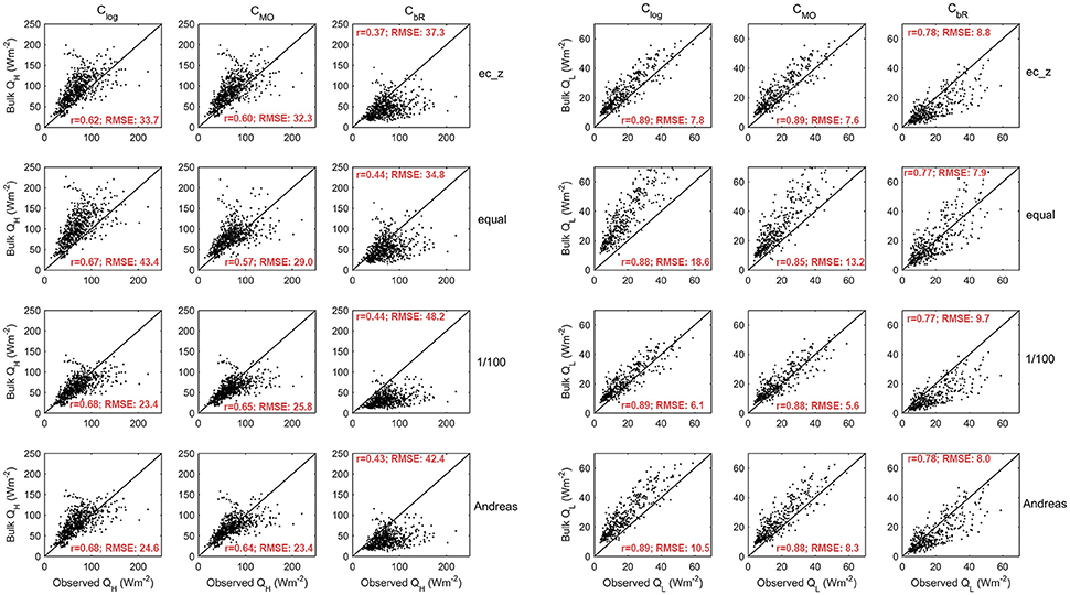
Figure 7. Performance of the tested bulk methods in modeling the EC-observed turbulent fluxes of sensible and latent heat.

Discussion

Energy Balance Observation and Closure

The strong performance of the model in replicating the recorded ablation rates gives a high level of confidence in the successful capture and closure of the SEB by the employed observation and correction methods. The trend of the modeled surface height over the 47 days (Figure 4A) shows no systematic bias to under or over-estimate when compared with the observed values, resulting in matching net values at the end of the study (−2.74 m). While good performance is also noted in the daily and 30 min ablation estimates, there are a number of pronounced periods where modeled values substantially differ from observations. Examining the daily timescale (Figure 4C), the days with the largest model differences are DOY 193 (+0.036 m), DOY 210 (−0.03 m), DOY 226 (+0.053 m), and DOY 234 (−0.034 m). In most cases, however, these differences can be attributed to observation error. Accidental compression of the snow underneath the sonic ranger during installation prior to DOY 193 resulted in a higher snow density and smaller observed height changes, while a review of camera imagery detected a clear tilting of the sonic ranger mast on both DOY 226 and 234, with the mast tilting forward and upslope on DOY 226 (sensor closer to the surface) and backward and downslope on DOY 234 (sensor further from the surface). DOY 210 was the day with the largest observed ablation and mean surface energy flux (288.8 Wm⁻²), but recorded 30% more ablation than DOY 197, which received just 1% less energy (285.5 Wm⁻²). Camera footage from DOY 210 may indicate the enhancement of a small meltwater stream within the footprint of the sonic ranger, which may have increased mass removal during this period, but the camera angle prevents definitive confirmation of this. Evaluating the SEB model performance with confirmed ranger error days removed (DOY 193, 226, 234) results in a marked improvement with r: 0.95 and RMSE: 0.01 m/day.

The SEB model offers good performance at 30 min resolution (r: 0.78; RMSE: 0.001 m/30 min, with aforementioned error days removed). The most prominent anomaly in the comparison between observed and modeled data at this timescale is the increase in surface height frequently observed by the ranger during night hours (negative values in Figure 4B). With only one period of trace snowfall during the study, accumulation does not account for these increases (mean increase of 0.003 m/night). A possible explanation for this behavior is the settling of the ranger mast into the warm surface ice; a signal that only becomes visible in the height data in the evening when surface ablation is reduced. With reduced heat and meltwater input into the borehole as the night progresses, this process slows, and at dawn, its signal is once again masked by ablation. This may also explain why the anomaly appears to be strongest in the later stages of the season (maximum increase of 0.03 m/night), when the base of the mast is closer to the surface, and more exposed to surface heat and under greater tilt leverage. An array of sonic rangers around the observation site would be a useful addition to future studies by providing additional data sources when sensor tilting or noise are obscuring the surface height signal from one. It would also help to constrain the likely range of ablation values at the glacier site where substantial variation in ablation can exist over small spatial scales.

In general, the partitioning of the observed SEB is in line with the values determined in existing studies on other mid-latitude glaciers (e.g., Hock and Holmgren, 1996; Greuell and Smeets, 2001). Q_N dominated melt energy, with its magnitude and variability primarily influenced by the net shortwave radiation (S_N), as shown in Figure 5B. Low cloud amount (reduced L_i fluxes) and a steadily melting surface (large magnitude L_o fluxes) resulted in a negative net longwave radiation flux (L_N), on average. The relatively large energy contribution provided by Q_H was maintained by the strong and consistently positive temperature gradients between the air and surface, and persistent downslope winds. Q_R provided a negligible contribution (<1%) to the total melt energy over the recorded period. However, over daily and sub-daily timescales, Q_R was observed to have a considerable influence on SEB and ablation during heavy rainfall. On July 19th (DOY 200), persistent heavy rain (daily total: 109.8 mm) resulted in a relatively large Q_R contribution of 20.1% to the daily energy flux (Figure 5A). There are previously mentioned uncertainties in the Q_R values arising from the observed rainfall rates, and the assumption made in Equation (13) that drop temperature is in equilibrium with air temperature. However, the general findings from this study show that, on daily and sub-daily timescales, Q_R has the potential to be a significant flux during extreme rain events; a phenomenon projected to become more frequent in a warmer climate (IPCC, 2013). Despite extensive cloud cover on DOY 200, daily ablation (0.058 m w.e.) was above the seasonal average (0.049 m w.e./day), with the non-radiative fluxes dominating Q_M (57.6%), highlighting the importance of accurate observation or estimation of non-radiative fluxes on glaciers (Fausto et al., 2016).

Bulk Method Evaluation

The initial step in evaluating the bulk method and its uncertainties was to compare roughness lengths calculated from the observed EC data with those commonly assumed for glacier surfaces. Despite extensive filtering, the scatter of the EC-derived roughness values was large over time (Figure 6) due to a dependence on a range of mean and turbulent variables in their calculation, as noted in previous studies (Andreas et al., 2010). The mean z_0v value from ec_z over the first 4 day period (10^−3.8 m) was found to be 1.6 orders of magnitude smaller than for the remaining 41 days (10^−2.2 m). The area upwind from the station (i.e., turbulent flux footprint area) was predominately snow covered during this initial period, and may have presented a smoother surface to the flow than the subsequent ice surface. This observed value for snow is similar to the assumed z_0v of 10⁻⁴ m, but there is close to an order of magnitude difference between the observed and assumed (10⁻³ m) values for the ice surface. A z_0v value of 10^−2.2 m is in the upper range of existing observations on glacier ice (Brock et al., 2006), and in line with measurements over rough, heavily gullied ice surfaces (Smeets et al., 1999). This relatively large roughness value may indicate the influence of the meltwater-enhanced channel network observed to develop on the surface of Nordic glacier during the study.

Rather than being equal to z_0v, the observed scalar roughness lengths were found to be several orders of magnitude smaller, as has been noted in previous studies (Beljaars and Holtslag, 1991; Smeets et al., 1998). The assumption that the scalar values are equal to each other was not observed at this site, with mean z_0q (10^{−6.0 ± 0.8} m) 1.4 orders of magnitude smaller than mean z_0t (10^{−4.6 ± 1.1} m). However, only 11 data points were available for z_0q after filtering, and there was substantial variability and overlapping of both sets of scalar values (Figure 8A). Substituting the ec_z values for z_0v into the tested roughness length schemes, the equal method overestimates both of the scalar roughness lengths, in some cases, by up to 4 orders of magnitude. The 1/100 method gives a reasonable mean value for z_0t while overestimating z_0q. The observed data for z_0t/z_0v show general agreement with the curve of the Andreas (1987) model (Figure 8B), but with a tendency for z_0t to be underestimated by the model (mean: 10^−5.3 m). The Andreas model was developed over snow and sea ice, which normally present a smoother surface to the flow than glacier ice. Smeets and van den Broeke (2008) proposed an adaption to this model for rougher ice surfaces (z_0v > 10⁻³ m). This scheme was also applied to the observed z_0v data, resulting in a calculated mean scalar roughness length value of 10^−3.2 m. Therefore, the observed z_0t values for this study lie mostly between both schemes. z_0q is overestimated by both methods, but shows best agreement with the Andreas model, with a modeled mean value of 10^−4.9 m (Figure 8C). Relations between mean meteorological variables (e.g., air temperature, relative humidity) and the scalar roughness lengths have been proposed in previous studies (Calanca, 2001; Park et al., 2010). However, such relationships were not evident in this data set. For the roughness length results in general, the limited number of data points available for analysis due to the persistent stable atmospheric conditions makes it difficult to draw definitive conclusions. An expanded study over more than one location, and with a greater number of measurements during neutral conditions, would be beneficial.

FIGURE 8

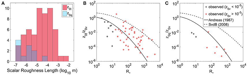
Figure 8. (A) Distribution of the EC-derived scalar roughness length values (overlapping regions in purple), and the relationships between the roughness Reynolds number and the (B) z_0t/z_0v and (C) z_0q/z_0v ratios, as proposed by Andreas (1987), and Smeets and van den Broeke (SvdB) (2008), and as observed in this study (during near-neutral conditions).

Assuming the ec_z values to be representative of the glacier surface, applying these roughness lengths to the three tested bulk transfer coefficients allows for an assessment of the performance of each stability scheme in returning flux values similar to those observed (Table 3). With no stability functions, C_log does not account for the suppression of turbulence that would theoretically be expected in the predominately stable surface layer at the site. The iterative scheme used to determine L for the C_MO method (Equation 22) was found to overestimate when compared with EC-derived values of L_ec (Figure 9B). As a result, stability is underestimated, and the suppression applied by the stability functions is insufficient. Similar overestimation of L has been observed in a recent comparison on a glacier surface by Radić et al. (2017). For daily mean fluxes (with only ideal EC measurement periods included), the performance of C_MO is significantly improved, with correlation values for Q_H and Q_L of 0.88 and 0.95, respectively (Figure 10). As mentioned, there was substantial observed variability around the mean ec_z values used in the bulk calculations. To test the sensitivity of the modeled fluxes to this variability, Monte Carlo analysis was applied to the utilized roughness lengths. For each 30 min C_MO flux calculation, 10,000 runs were performed where each of the three roughness lengths were selected at random from normally distributed populations with the means and standard deviations of the corresponding ec_z values. The standard deviation of the daily means from these runs are presented as error bars on the modeled flux values in Figure 10. Allowing for this sensitivity to roughness length input, periods of flux overestimation remain, being most pronounced during days with combined conditions of strong stability, large near-surface air temperature gradients, and relatively strong downslope winds, indicative of katabatic flow. Throughout the study period, the strengthening of the near-surface temperature gradient was observed to correspond with a strengthening of the downslope airflow that dominated the observed wind direction (Figure 9A). The possible development during very stable conditions of a low-level wind maximum near measurement height may have decoupled turbulence generation from the surface, and invalidated the assumptions of Monin-Obukhov similarity theory, such as a constant flux layer related to near surface gradients (Van der Avoird and Duynkerke, 1999; Denby and Greuell, 2000; Grisogono and Oerlemans, 2001; Parmhed et al., 2004). Simultaneous wind and momentum flux profile measurements at the study site would be required to confirm the presence and height of a low-level wind maximum, and to identify it as the cause of the error postulated above.

FIGURE 9

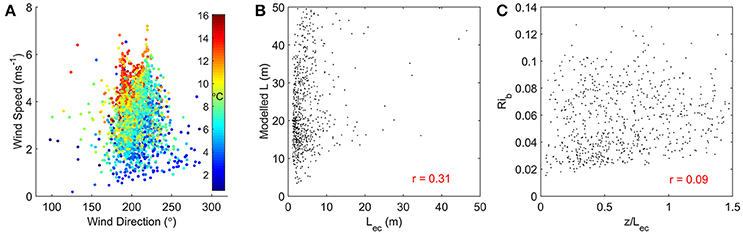
Figure 9. (A) Relationship between observed 30 min wind direction, wind speed, and 2 m air temperature, (B) observed vs. modeled Obukhov length values, and (C) observed stability parameter values vs. the calculated bulk Richardson number. Only values from periods with “ideal” EC conditions are displayed here.

FIGURE 10

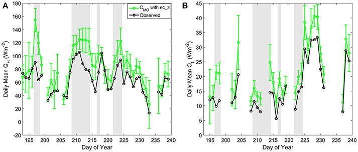
Figure 10. Daily means of observed turbulent heat fluxes (black) and C_MO modeled fluxes using ec_z roughness lengths (green), for (A) Q_H, and (B) Q_L. Periods with suspected low-level katabatic wind maximums are shaded gray. Daily means only include the 30 min periods which pass the filters for ideal EC measurement conditions. Error bars on the modeled fluxes represent the standard deviation of the daily means from the Monte Carlo sensitivity analysis.

As the majority of studies on glaciers do not have access to direct observations of turbulence or roughness lengths, the performances of the bulk methods were also evaluated using existing assumed roughness values and schemes. As noted, the combination of C_log and the 1/100 roughness scheme provides the best performing assumed bulk method. C_log may have been expected to overestimate the fluxes in the predominately stable atmospheric conditions during the study. However, implementing a roughness scheme with a mean z_0v substantially smaller than the actual value determined for the surface reduces the magnitude of the fluxes calculated by this method. The small underestimation of Q_H can be attributed to implementing a slightly smaller mean z_0t than was observed, and conversely for Q_L, with a slightly larger mean z_0q. C_bR displays the poorest performance of all bulk methods; its stability function excessively suppressing both fluxes, and yielding low correlation values, particularly for Q_H. Q_L is well modeled by C_bR when coupled with the equal roughness scheme; the excessive suppression being balanced by a large z_0q value. While showing general agreement that conditions were predominately stable (Figure 9C), the bulk Richardson number (mean = 0.06 ± 0.02) does not correlate with the observed stability parameter $\frac{z}{L_{ec}}$ from the EC data (r = 0.09). C_MO returns better performance than C_bR. Q_H is relatively well modeled when coupled with the Andreas roughness model; the small assumed z_0v compensated by an overestimated z_0t, and insufficient turbulence suppression by C_MO. A similar situation using the 1/100 method results in a well modeled Q_L by C_MO.

Effect of Parameterization on SEB Closure

The implementation of direct observations for all eight fluxes in the melt model returned results that effectively closed the SEB of the study site. However, as complete flux observations on glacier surfaces are rarely available, the effects of simplifying and parameterizing aspects of the SEB are also considered. Some of the most basic assumptions and values used in SEB studies, namely, negligible Q_R and Q_G, and constant T_s (0°C) and L_o (315.6 Wm⁻², with unity emissivity), were applied to the model, and found to have little effect on performance when applied individually or in combination (r = 0.94; RMSE = 0.01 m/day, for daily surface height change). This result is specific to this field study, and may differ significantly if applied to sites other than continental, temperate glaciers. It should also be noted that due to the discussed adjustments made to the L_o data, the assumption of constant T_s has already been partially applied to the model. The impact of parameterizing the turbulent heat fluxes was also assessed, and the choice of bulk method used was found to have a major influence on closure performance. Figure 11A displays the daily deviation from Q_M (obtained through the fully observed SEB) for simplified SEB models with a range of previously discussed bulk methods implemented (in addition to the basic assumptions above). The returned daily model values can vary by ±40%, depending on the scheme utilized, resulting in differences of up to ±0.5 m from the sonic ranger observed (or full SEB modeled) cumulative surface melt over the study period (Figure 11B).

FIGURE 11

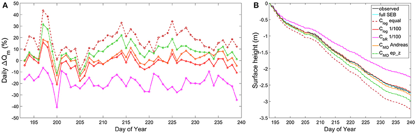
Figure 11. (A) Deviation from daily Q_M for a range of simplified SEB models with varying turbulence parameterizations (stability and roughness scheme identified), and (B) the cumulative effect of these deviations on modeled surface height over the study period. Each of the simplified models also assumes negligible Q_R and Q_G, and constant T_s and L_o.

Conclusions

A method to observe the complete surface energy balance of a glacier has been employed in this study to investigate the ablation characteristics of a mid-latitude, alpine glacier. Direct observations of S_i, S_r, L_i, L_o, Q_H, Q_L, Q_R, and Q_G were implemented in an SEB model to produce half-hourly estimates of surface ablation, which were then compared with the observed ablation values over a 47 day period. In addition, the Q_H and Q_L observations, obtained using eddy covariance measurements, were used to evaluate the performance of a range of bulk method parameterization techniques commonly used in glacier SEB studies, where direct measurement of the turbulent fluxes is rare.

In general, the modeled ablation values showed excellent agreement with the observed data, accurately estimating the total surface height loss over the period (2.74 m), and providing good performance at daily (r: 0.95; RMSE: 0.01 m/day) and 30 min (r: 0.78; RMSE: 0.001 m/30 min) timescales. The observation system effectively captured and closed the surface energy balance of the glacier, and maintained continuous operation throughout the study period, indicating it to be a useful system for investigating glacier-atmosphere interactions. The SEB partitioning of Nordic Glacier was found to be similar to other mid-latitude glaciers, with net radiation dominating Q_M (65.2%). Q_H was also observed to be an important contributor to melt energy (29.7%), underlining the need to accurately account for the turbulent heat fluxes. At daily and sub-daily timescales, Q_R was observed to be a substantial energy source during heavy rain events (up to 20% of daily melt energy).

EC-derived measurements of z_0v obtained for the study site showed general agreement with previously observed values on glaciers, with a distinct difference in mean z_0v between periods with a snow (10^{−3.8 ± 1.7} m) and ice (10^{−2.2 ± 0.7} m) covered surface. The z_0v value for ice is close to an order of magnitude larger than that commonly used in the literature for similar surfaces (10⁻³ m). This gives emphasis to the importance of site-specific values, particularly when the impact of roughness length selection on the magnitude of the calculated fluxes, as observed in this study, is considered. The observed mean scalar roughness length values of z_0t (10^{−4.6 ± 1.1} m) and z_0q (10^{−6.0 ± 0.8} m) differ by several orders of magnitude from z_0v, disagreeing with the common assumption of equal momentum and scalar roughness lengths. Values for z_0t showed reasonable agreement with the z_0v/100 ratio and the surface renewal models of Andreas (1987) and Smeets and van den Broeke (2008).

Three of the stability schemes most commonly used in the bulk method were evaluated in this study through comparison of the parameterized fluxes with the EC-observed values. When implemented with the roughness length values calculated for the study surface (ec_z), each of the tested methods either over- or underestimated the turbulent fluxes for the stable atmospheric conditions on the glacier. The C_MO method returned the strongest performance overall, showing significant correlation with the observed fluxes over daily time scales, but a tendency to underestimate stability and the required turbulence suppression. Flux overestimation was most pronounced during days with a suspected low-level wind maximum near measurement height, when the associated decoupling of turbulence generation from the surface may have invalidated Monin-Obukhov similarity theory. Utilizing a range of unobserved, assumed roughness length values with the above stability schemes led, in a few cases, to a balancing of errors; the inaccuracies in the roughness values counteracting the deficiencies in the stability functions. As a result, relatively good performance in modeling the turbulent fluxes was achieved using ice and snow z_0v values from the literature (10⁻³ m and 10⁻⁴ m), and a bulk method that assumes neutral conditions (C_log) and a 1/100 roughness length ratio. However, the above technique is not firmly based on the physical characteristics of the study surface and boundary layer, and its transferability to other glaciers and seasons remains uncertain. As observed in this study, the choice of bulk method can dramatically influence the performance of an SEB model (±40% of daily Q_M), and a systematic approach for selecting the most accurate method for given conditions on a glacier requires further development.

Author Contributions

NF performed the fieldwork, model development, and analysis for the study, and wrote the manuscript. VR supervised the study, provided financial and field support and contributed to manuscript preparation. BM provided logistical and minor financial support, and provided editorial suggestions on the manuscript.

Funding

Funding support for this study was provided through the Natural Sciences and Engineering Research Council of Canada [Discovery grants to VR and BM], the Canada Research Chairs Program, and the Columbia Basin Trust.

Conflict of Interest Statement

The authors declare that the research was conducted in the absence of any commercial or financial relationships that could be construed as a potential conflict of interest.

Acknowledgments

The authors wish to thank Steve Conger, Tannis Dakin, and Federico Ponce for logistical support, Zoran Nesic for assistance with station design and sensor calibration, Jörn Unger for his work on the quadpod construction, and Ben Pelto for provision of the LiDAR base map.

References

Anderson, B., Mackintosh, A., Stumm, D., and Fitzsimons, S. J. (2010). Climate sensitivity of a high-precipitation glacier in New Zealand. J. Glaciol. 56, 114–128. doi: 10.3189/002214310791190929

CrossRef Full Text | Google Scholar

Andreas, E. L. (1987). A theory for the scalar roughness and the scalar transfer coefficients over snow and sea ice. Boundary-Layer Meteorol. 38, 159–184. doi: 10.1007/BF00121562

CrossRef Full Text | Google Scholar

Andreas, E. L., Persson, P. O. G., Jordan, R. E., Horst, T. W., Guest, P. S., Grachev, A. A., et al. (2010). Parameterizing turbulent exchange over sea ice in winter. J. Hydrometeorol. 11, 87–104. doi: 10.1175/2009JHM1102.1

CrossRef Full Text | Google Scholar

Andreassen, L. M., Van Den Broeke, M. R., Giesen, R. H., and Oerlemans, J. (2008). A 5 year record of surface energy and mass balance from the ablation zone of Storbreen, Norway. J. Glaciol. 54, 245–258. doi: 10.3189/002214308784886199

CrossRef Full Text | Google Scholar

Arnold, N. S., Rees, W. G., Hodson, A. J., and Kohler, J. (2006). Topographic controls on the surface energy balance of a high Arctic valley glacier. J. Geophys. Res. 111:F02011. doi: 10.1029/2005JF000426

CrossRef Full Text | Google Scholar

Aubinet, M. (2008). Eddy covariance CO₂ flux measurements in nocturnal conditions: an analysis of the problem. Ecol. Appl. 18, 1368–1378. doi: 10.1890/06-1336.1

PubMed Abstract | CrossRef Full Text | Google Scholar

Aubinet, M., Vesala, T., and Papale, D. (2012). Eddy Covariance: A Practical Guide to Measurement and Data Analysis. Dordrecht: Springer. doi: 10.1007/978-94-007-2351-1

CrossRef Full Text | Google Scholar

Beljaars, A. C. M., and Holtslag, A. A. M. (1991). Flux parameterization over land surfaces for amospheric models. J. Appl. Meteorol. 30, 327–341. doi: 10.1175/1520-0450(1991)030<0327:FPOLSF>2.0.CO;2

CrossRef Full Text | Google Scholar

Brock, B. W., Mihalcea, C., Kirkbride, M. P., Diolaiuti, G., Cutler, M. E. J., and Smiraglia, C. (2010). Meteorology and surface energy balance fluxes in the 2005–2007 ablation seasons at the Miage debris-covered glacier, Mont Blanc Massif, Italian Alps. J.Geophys. Res. 115:D09106. doi: 10.1029/2009JD013224

CrossRef Full Text | Google Scholar

Brock, B. W., Willis, I. C., and Sharp, M. J. (2006). Measurement and parameterization of aerodynamic roughness length variations at Haut Glacier d'Arolla, Switzerland. J. Glaciol. 52, 281–297. doi: 10.3189/172756506781828746

CrossRef Full Text | Google Scholar

Burba, G. (2013). Eddy Covariance Method for Scientific, Industrial, Agricultural, and Regulatory Applications. Lincoln, NE: LI-COR Biosciences.

Google Scholar

Calanca, P. (2001). A note on the roughness length for temperature over melting snow and ice. Q. J. R. Meteorol. Soc. 127, 255–260. doi: 10.1002/qj.49712757114

CrossRef Full Text | Google Scholar

Campbell Scientific Inc. (2013). IRGASON Integrated C0₂/H₂0 Open-Path Gas Analyzer and 3D Sonic Anemometer Manual. Edmonton, AB: Campbell Scientific (Canada) Corp.

Campbell Scientific Inc. (2014). SR50A Sonic Ranging Sensor Instruction Manual. Edmonton, AB: Campbell Scientific (Canada) Corp.

Clarke, G. K. C., Jarosch, A. H., Anslow, F. S., Radić, V., and Menounos, B. (2015). Projected deglaciation of western Canada in the twenty-first century, Nat. Geosci. 8, 372–377. doi: 10.1038/ngeo2407

CrossRef Full Text | Google Scholar

Columbia Basin Trust (2017). The Basin. Available online at: http://www.cbt.org/The_Basin/

Conway, J. P., and Cullen, N. J. (2013). Constraining turbulent heat flux parameterization over a temperate maritime glacier in New Zealand. Annal. Glaciol. 54, 41–51. doi: 10.3189/2013AoG63A604

CrossRef Full Text | Google Scholar

Cullen, N. J., Mölg, T., Kaser, G., Steffen, K., and Hardy, D. R. (2007). Energy-balance model validation on the top of Kilimanjaro, Tanzania, using eddy covariance data. Annal. Glaciol. 46, 227–233. doi: 10.3189/172756407782871224

CrossRef Full Text | Google Scholar

Dadic, R., Mott, R., Lehning, M., Carenzo, M., Anderson, B., and Mackintosh, A. (2013). Sensitivity of turbulent fluxes to wind speed over snow surfaces in different climatic settings. Adv. Water Res. 55, 178–189. doi: 10.1016/j.advwatres.2012.06.010

CrossRef Full Text | Google Scholar

Denby, B., and Greuell, W. (2000). The use of bulk and profile methods for determining surface heat fluxes in the presence of glacier winds. J. Glaciol. 46, 445–452. doi: 10.3189/172756500781833124

CrossRef Full Text | Google Scholar

Devine, K. A., and Mekis, E. (2008). Field accuracy of Canadian rain measurements. Atmosphere-Ocean 46, 213–227. doi: 10.3137/ao.460202

CrossRef Full Text | Google Scholar

Duchon, C., and Biddle, C. J. (2010). Undercatch of tipping-bucket gauges in high rain rate events. Adv. Geosci. 25, 11–15. doi: 10.5194/adgeo-25-11-2010

CrossRef Full Text | Google Scholar

Dyer, A. J. (1974). A review of flux-profile relationships. Boundary-Layer Meteorol. 7, 363–372. doi: 10.1007/BF00240838

CrossRef Full Text | Google Scholar

Fausto, R. S., van As, D., Box, J. E., Colgan, W., Langen, P. L., and Mottram, R. H. (2016). The implication of nonradiative energy fluxes dominating Greenland ice sheet exceptional ablation area surface melt in 2012. Geophys. Res. Lett. 43, 2649–2658. doi: 10.1002/2016GL067720

CrossRef Full Text | Google Scholar

Finkelstein, P. L., and Sims, P. F. (2001). Sampling error in eddy correlation flux measurements. J. Geophys. Res. 106, 3503–3509. doi: 10.1029/2000JD900731

CrossRef Full Text | Google Scholar

Fitzpatrick, N. (2007). Uncertainty in Stevenson Screen Temperature Measurements [Master's Thesis], University of Reading (Reading), 73.

Foken, T. (2008). Micro-meteorology. Berlin: Springer.

Giesen, R. H., Andreassen, L. M., Oerlemans, J., and Van Den Broeke, M. R. (2014). Surface energy balance in the ablation zone of Langfjordjøkelen, an arctic, maritime glacier in northern Norway. J. Glaciol. 60, 57–70. doi: 10.3189/2014JoG13J063

CrossRef Full Text | Google Scholar

Gillet, S., and Cullen, N. J. (2011). Atmospheric controls on summer ablation over Brewster Glacier, New Zealand. Int. J. Climatol. 31, 2033–2048. doi: 10.1002/joc.2216

CrossRef Full Text | Google Scholar

Greuell, W., and Smeets, P. (2001). Variations with elevation in the surface energy balance on the Pasterze (Austria). J. Geophys. Res. 106, 31717–31727. doi: 10.1029/2001JD900127

CrossRef Full Text | Google Scholar

Grisogono, B., and Oerlemans, J. (2001). katabatic flow: analytic solution for gradually varying eddy diffusivities. J. Atmos. Sci. 58, 3349–3354. doi: 10.1175/1520-0469(2001)058<3349:KFASFG>2.0.CO;2

CrossRef Full Text | Google Scholar

Harrison, R. G. (2010). Natural ventilation effects on temperatures within Stevenson screens. Q. J. R. Meteorol. Soc. 136, 253–259. doi: 10.1002/qj.537

CrossRef Full Text | Google Scholar

Hay, J. E., and Fitzharris, B. B. (1988). A comparison of energy balance and bulk aerodynamic approaches for estimating glacier melt. J. Glaciol. 34, 145–153. doi: 10.1017/S0022143000032172

CrossRef Full Text | Google Scholar

Hock, R. (2005). Glacier melt: a review of processes and their modelling. Prog. Phys. Geogr. 29, 362–391. doi: 10.1191/0309133305pp453ra

CrossRef Full Text | Google Scholar

Hock, R., and Holmgren, B. (1996). Some aspects of energy balance and ablation of Storglaciären, northern Sweden. Geogr. Ann. 78, 121–131. doi: 10.2307/520974

CrossRef Full Text | Google Scholar

Hock, R., and Holmgren, B. (2005). A distributed surface energy-balance model for complex topography and its application to Storglaciären, Sweden. J. Glaciol. 51, 25–36. doi: 10.3189/172756505781829566

CrossRef Full Text | Google Scholar

Hock, R., and Schroff, K. (2004). “Difference between ventilated and unventilated temperature measurements over snow surfaces,” in Automatic Weather Stations on Glaciers – Lessons to be learned Extended abstracts, eds J. Oerlemans and C. H. Tijm-Reijmer (Utrecht: Institute for Marine and Atmospheric Research), 56–58.

Ibrom, A., Dellwik, E., Flyvbjerg, H., Jensen, N. O., and Pilegaard, K. (2007). Strong low-pass filtering effects on water vapor flux measurements with closed-path eddy correlation systems. Agric. For. Meteorol. 147, 140–156. doi: 10.1016/j.agrformet.2007.07.007

CrossRef Full Text | Google Scholar

IPCC (2013). “Summary for Policymakers,” in Climate Change 2013: The Physical Science Basis. Contribution of Working Group I to the Fourth Assessment Report of the Intergovernmental Panel on Climate Change, eds S. Solomon, D. Qin, M. Manning, Z. Chen, M. Marquis, K. B. Averyt, M. Tignor, and H. L. Miller (Cambridge, New York, NY: Cambridge University Press), 1–18.

Jonsell, U., Hock, R., and Holmgren, B. (2003). Spatial and temporal variations in albedo on Storglaciären, Sweden. J. Glaciol. 49, 59–68. doi: 10.3189/172756503781830980

CrossRef Full Text | Google Scholar

Jost, G., Moore, R. D., Menounos, B., and Wheate, R. (2012). Quantifying the contribution of glacier runoff to streamflow in the upper Columbia River Basin, Canada. Hydrol. Earth Syst. Sci. 16, 849–860. doi: 10.5194/hess-16-849-2012

CrossRef Full Text | Google Scholar

Kaimal, J. C., and Gaynor, J. E. (1991). Another look at sonic thermometry. Boundary-Layer Meteorol. 56, 401–410. doi: 10.1007/BF00119215

CrossRef Full Text | Google Scholar

Kipp and Zonen (2009). CNR 4 Net Radiometer Instruction Manual. Delft: Kipp & Zonen.

Konzelmann, T., and Braithwaite, R. J. (1995). Variations of ablation, albedo and energy balance at the margin of the Greenland ice sheet, Kronprins Christian Land, eastern north Greenland. J. Glaciol. 41, 174–182. doi: 10.1017/S002214300001786X

CrossRef Full Text | Google Scholar

Lee, X., Massman, W., and Law, B. (2004). Handbook of Micrometeorology: A Guide for Surface Flux Measurement and Analysis. Dordrecht: Kluwer Academic Publishers.

Google Scholar

Li, Z., Lyu, S., Zhao, L., Wen, L., Ao, Y., and Wang, S. (2016). Turbulent transfer coefficient and roughness length in a high-altitude lake, Tibetan Plateau. Theor. Appl. Climatol. 124, 723–735. doi: 10.1007/s00704-015-1440-z

CrossRef Full Text | Google Scholar

Litt, M., Sicart, J. E., Helgason, W. D., and Wagnon, P. (2015). Turbulence characteristics in the atmospheric surface layer for different wind regimes over the tropical zongo glacier (Bolivia, 16°S). Boundary-Layer Meteorol. 154, 471–495. doi: 10.1007/s10546-014-9975-6

CrossRef Full Text | Google Scholar

Mekonnen, G. B., Matula, S., and Doležal, F. (2015). Adjustment to rainfall measurement undercatch with a tipping-bucket rain gauge using ground-level manual gauges. Meteorol. Atmos. Phys. 127, 241–256. doi: 10.1007/s00703-014-0355-z

CrossRef Full Text | Google Scholar

Mölg, T., and Hardy, D. R. (2004). Ablation and associated energy balance of a horizontal glacier surface on Kilimanjaro, J. Geophys. Res. 109:D16104. doi: 10.1029/2003JD004338

CrossRef Full Text | Google Scholar

Moncrieff, J. B., Clement, R., Finnigan, J., and Meyers, T. (2004). “Averaging, detrending and filtering of eddy covariance time series,” in Handbook of Micrometeorology: A Guide For Surface Flux Measurements, eds X. Lee, W. Massman, and B. Law (Dordrecht: Kluwer Academic), 7–31.

Google Scholar

Monin, A. S., and Obukhov, A. M. (1954). Basic laws of turbulent mixing in the surface layer of the atmosphere. Tr. Akad. Nauk SSSR Geophiz. Inst. 24, 163–187.

Google Scholar

Munro, D. S. (1989). Surface roughness and bulk heat transfer on a glacier: comparison with Eddy correlation. J. Glaciol. 35, 343–348. doi: 10.1017/S0022143000009266

CrossRef Full Text | Google Scholar

Obleitner, F. (2004). “On the performance of unaspirated, plate-shielded thermometer screens,” in Automatic Weather Stations on Glaciers–Lessons to be Learned Extended Abstracts, eds J. Oerlemans and C. H. Tijm-Reijmer (Utrecht: Institute for Marine and Atmospheric Research), 76–82.

Google Scholar

Park, S. J., Park, S. U., and Ho, C. H. (2010). Roughness length of water vapor over land surfaces and its influence on latent heat flux. Terr. Atmos. Ocean. Sci. 21, 855–867. doi: 10.3319/TAO.2009.11.13.01(Hy)

CrossRef Full Text | Google Scholar

Parmhed, O., Oerlemans, J., and Grisogono, B. (2004). Describing surface fluxes in katabatic flow on Breidamerkurjökull, Iceland, Q. J. R. Meteorol. Soc. 130, 1137–1151. doi: 10.1256/qj.03.52

CrossRef Full Text | Google Scholar

Radić, V., Menounos, B., Shea, J., Fitzpatrick, N., Tessema, M. A., and Dery, S. J. (2017). Evaluation of different methods to model near-surface turbulent fluxes for an alpine glacier in the Cariboo Mountains, BC, Canada. Cryosphere Discuss. 1–39. doi: 10.5194/tc-2017-80

CrossRef Full Text | Google Scholar

Sicart, J. E., Wagon, P., and Ribstein, P. (2005). Atmospheric controls of the heat balance of Zongo Glacier (16°S, Bolivia), J. Geophys. Res. 110:D12106. doi: 10.1029/2004JD005732

CrossRef Full Text | Google Scholar

Smeets, C. J. P. P., Duynkerke, P. G., and Vugts, H. F. (1998). Turbulence characteristics of the stable boundary layer over a mid-latitude glacier. Part I: a combination of katabatic and large-scale forcing. Boundary-Layer Meteorol. 87, 117–145. doi: 10.1023/A:1000860406093

CrossRef Full Text | Google Scholar

Smeets, C. J. P. P., Duynkerke, P. G., and Vugts, H. F. (1999). Observed wind profiles and turbulence fluxes over an ice surface with changing surface roughness. Boundary-Layer Meteorol. 92, 99–121. doi: 10.1023/A:1001899015849

CrossRef Full Text | Google Scholar

Smeets, C. J. P. P., and van den Broeke, M. R. (2008). The parameterisation of scalar transfer over rough ice. Boundary-Layer Meteorol. 128, 339–355. doi: 10.1007/s10546-008-9292-z

CrossRef Full Text | Google Scholar

Stull, R. B. (1988). An Introduction to Boundary Layer Meteorology. Dordrecht: Kluwer Academic Publishers. doi: 10.1007/978-94-009-3027-8

CrossRef Full Text | Google Scholar

Van As, D. (2011). Warming, glacier melt and surface energy budget from weather station observations in the Melville Bay region of northwest Greenland. J. Glaciol. 57, 208–220. doi: 10.3189/002214311796405898

CrossRef Full Text | Google Scholar

Van den Broeke, M., Reijmer, C., van As, D., van de Wal, R., and Oerlemans, J. (2005). Seasonal cycles of Antarctic surface energy balance from automatic weather stations. Annals Glaciol. 41, 131–139. doi: 10.3189/172756405781813168

CrossRef Full Text | Google Scholar

Van den Broeke, M., van As, D., Reijmer, C., and van de Wal, R. (2004). Assessing and improving the quality of unattended radiation observations in Antarctica. J. Atmos. Oceanic Tech. 21, 1417–1431. doi: 10.1175/1520-0426(2004)021<1417:AAITQO>2.0.CO;2

CrossRef Full Text | Google Scholar

Van der Avoird, E., and Duynkerke, P. G. (1999). Turbulence in a katabatic flow. Boundary-Layer Meteorol. 92, 37–63. doi: 10.1023/A:1001744822857

CrossRef Full Text | Google Scholar

Webb, E. K. (1970). Profile relationships: the log-linear range, and extension to strong stability. Q. J. R. Meteorol. Soc. 96, 67–90. doi: 10.1002/qj.49709640708

CrossRef Full Text | Google Scholar

Webb, E. K., Pearman, G. I., and Leuning, R. (1980). Correction of flux measurements for density effects due to heat and water vapour transfer. Q. J. R. Meteorol. Soc. 106, 85–100. doi: 10.1002/qj.49710644707

CrossRef Full Text | Google Scholar

Wilczak, J. M., Oncley, S. P., and Stage, S. A. (2001). Sonic anemometer tilt correction algorithms. Boundary-Layer Meteorol. 99, 127–150. doi: 10.1023/A:1018966204465

CrossRef Full Text | Google Scholar

World Meteorological Organisation (WMO) (1983). Guide to Meteorological Instruments and Methods of Observation - WMO No.8. Geneva: World Meteorological Organisation.