The Polar WRF Downscaled Historical and Projected Twenty-First Century Climate for the Coast and Foothills of Arctic Alaska

Cai, Lei; Alexeev, Vladimir A.; Arp, Christopher D.; Jones, Benjamin M.; Liljedahl, Anna K.; Gädeke, Anne

doi:10.3389/feart.2017.00111

ORIGINAL RESEARCH article

Front. Earth Sci., 09 January 2018
Sec. Atmospheric Science
Volume 5 - 2017 | https://doi.org/10.3389/feart.2017.00111

The Polar WRF Downscaled Historical and Projected Twenty-First Century Climate for the Coast and Foothills of Arctic Alaska

Lei Cai¹^*

Benjamin M. Jones³

¹International Arctic Research Center, University of Alaska Fairbanks, Fairbanks, AK, United States
²Water and Environment Research Center, University of Alaska Fairbanks, Fairbanks, AK, United States
³U.S. Geological Survey, Alaska Science Center, Anchorage, AK, United States

Climate change is most pronounced in the northern high latitude region. Yet, climate observations are unable to fully capture regional-scale dynamics due to the sparse weather station coverage, which limits our ability to make reliable climate-based assessments. A set of simulated data products was therefore developed for the North Slope of Alaska through a dynamical downscaling approach. The polar-optimized Weather Research and Forecast (Polar WRF) model was forced by three sources: The ERA-interim reanalysis data (for 1979–2014), the Community Earth System Model 1.0 (CESM1.0) historical simulation (for 1950–2005), and the CESM1.0 projected (for 2006–2100) simulations in two Representative Concentration Pathways (RCP4.5 and RCP8.5) scenarios. Climatic variables were produced in a 10-km grid spacing and a 3-h interval. The ERA-interim forced WRF (ERA-WRF) proves the value of dynamical downscaling, which yields more realistic topographical-induced precipitation and air temperature, as well as corrects underestimations in observed precipitation. In summary, dry and cold biases to the north of the Brooks Range are presented in ERA-WRF, while CESM forced WRF (CESM-WRF) holds wet and warm biases in its historical period. A linear scaling method allowed for an adjustment of the biases, while keeping the majority of the variability and extreme values of modeled precipitation and air temperature. CESM-WRF under RCP 4.5 scenario projects smaller increase in precipitation and air temperature than observed in the historical CESM-WRF product, while the CESM-WRF under RCP 8.5 scenario shows larger changes. The fine spatial and temporal resolution, long temporal coverage, and multi-scenario projections jointly make the dataset appropriate to address a myriad of physical and biological changes occurring on the North Slope of Alaska.

Introduction

The air temperature is increasing and more so in the northern high latitude regions due to the polar amplification (Alexeev et al., 2005; Serreze and Francis, 2006; Barber et al., 2008). Annual mean surface air temperatures from observations and reanalysis datasets have increased more than 2.5°C poleward of 60°N since the 1970s, which is of over 1°C more warming than that in the mid-latitudes (30–60°N) (Johannessen et al., 2004). Arctic sea ice cover is declining more than 3 × 10⁵ km per decade (Serreze et al., 2007). The declining sea ice accounts for a positive surface albedo feedback, which acts as a contributing factor, though not the dominating one, to the polar amplification phenomenon (Serreze and Francis, 2006; Winton, 2006).

The exact mechanism of polar amplification is still under active discussion, but it is agreed that the rapidly increasing air temperature and the declining sea ice cover since the 1970s have led to substantial environmental changes to the pan-Arctic coastal regions. For example, the permafrost temperature in the western North American Arctic has warmed by 0.5–4°C since the 1970s (Romanovsky et al., 2010; Grosse et al., 2011), resulting in active layer thickening (Kane et al., 1991; Grosse et al., 2016) and permafrost degradation (Jorgenson et al., 2006; Lantz and Kokelj, 2008; Liljedahl et al., 2016). Other changes include, but are not limited to, thermokarst lake drainage (Plug et al., 2008; Jones et al., 2011; Jones and Arp, 2015; Lantz and Turner, 2015), thinner lake ice (Arp et al., 2012; Alexeev et al., 2016), longer unfrozen Arctic lake surface (Brown and Duguay, 2010), more lake surface evaporation (Hinzman and Kane, 1992; Arp et al., 2015), and extended growing season (Hinzman et al., 2005; Tape et al., 2006; Bhatt et al., 2008; Chapin et al., 2012). Post et al. (2009) pointed out that the amount and types of impacts are still underreported and the understanding of the underlying physical mechanisms are still lacking due to insufficient observations in the Arctic.

Climate monitoring in the Arctic have been restricted by the lack of observational sites that are sparsely distributed, and few of which are observing routinely (Shulski and Wendler, 2007). The observation accuracy is hard to maintain in such a harsh environment, especially for the solid precipitation observation that is usually underestimated by a factor of two or more (Groisman et al., 1991; Rasmussen et al., 2012; Liljedahl et al., 2017). Conventional snowfall measurements are underestimated for the reasons including high wind speeds and trace precipitation events (Black, 1954; Liston and Sturm, 2002; Rasmussen et al., 2012). Despite problems with cold season precipitation measurements, the observed long-term records of air temperature are reliable (Vose et al., 2007).

Numerical simulations complement the limited field observations in Alaska and other Arctic regions. The latest Earth System Models (ESMs) has improved significantly in retrieving climatic variables coupling the atmosphere, land, ocean, and ice models (de Boer et al., 2012; Mortin et al., 2013; Koenigk et al., 2014). Still, the typical one-degree grid spacing prevents ESMs from resolving more detailed weather like Mesoscale Convective Systems (MCSs) and topographical-induced precipitation. Dynamical downscaling using Regional Climate Models (RCMs) forced by reanalysis data and/or ESM output is one way to amplify the mesoscale features and to retrieve high-resolution climatic variables regionally (Wilby and Wigley, 1997). The North American Regional Climate Change Assessment Program (NARCCAP) is a dynamical downscaling program with the ensemble of GCM-RCM combinations that serves the high-resolution climate scenario needs for the North America (Mearns et al., 2013). The mesoscale framework in NARCCAP results in more extreme precipitation events compared to the GCMs, and becoming less deviated from observations (Gutowski et al., 2010; Wehner, 2013). Coordinated Regional climate Downscaling Experiment (CORDEX) is another project that employed dynamical downscaling over multiple regions of interest around the globe (Europe, South Africa, East Asia, etc.) (Giorgi et al., 2009). CORDEX addresses dynamical downscaling forced by the latest generation of GCMs that are archived in Coupled Model Intercomparison Project Phase 5 (CMIP5) instead of its earlier phase (CMIP3) is selected in NARCCAP (Giorgi et al., 2009; Taylor et al., 2012; Mearns et al., 2013).

Dynamically downscaled ERA-interim reanalysis data already exist for Alaska as a whole, with a grid spacing of 20 km using Weather Research and Forecast (WRF) model (Bieniek et al., 2016). Here, the modeling configuration is tuned to emphasize the general climate divisions of Alaska (e.g., interior Alaska vs. coastal regions) and the distribution/frequency of extreme events. Chukchi–Beaufort High-Resolution Atmospheric Reanalysis (CBHAR) is another WRF-based downscaling product that focuses on the Arctic Alaska and the adjacent oceanic area to its north with a 10-km grid spacing and 1-h output interval (Liu et al., 2014). By involving WRF-Data Assimilation (WRFDA) system that imports satellite data, CBHAR represents a refined wind field in the Chukchi and Beaufort Seas regions (Zhang et al., 2016). Yet, a downscaled high-resolution future projection dataset centering on the Arctic land of Alaska has, until now, been unavailable. Here our objectives are to produce and present fine temporal (3-hourly) and spatial (10 km) downscaled historical atmospheric data with multi-projections representing the differing scenarios (RCP4.5 and RCP8.5) of climate change in Arctic Alaska from 1950 up until 2099.

Methodology

Site Description

Our downscaled products center on the Arctic Coastal Plain of Alaska and the Northern foothills of the Brooks Range (Figure 1). We use the term “the North Slope of Alaska” to describe the part of Alaska approximately to the north of 69°N. The Brooks Range, which has quite a few mountain peaks higher than 2,000 meters in altitude acts as a barrier, preventing warm and wet air from the Bering Sea from reaching the North Slope of Alaska (Shulski and Wendler, 2007). The region has the lowest mean annual air temperatures (< −10°C) and annual precipitation (~150 mm) observed in Alaska, both of which decrease along a gradient from the Brooks Range foothill to the Northern coast of Alaska (Stafford et al., 2000; Bieniek et al., 2012). The polar days in summer and nights in winter reduce the diurnal variation of solar radiation down to a level <30% of that in the mid-latitudes (Maykut and Church, 1973). The weakened diurnal cycle excludes solar radiation from being the leading control of the diurnal cycle of air temperature. Instead, it is the cloud cover and low-level wind that primarily drive the diurnal cycle of air temperature during polar days and nights (Dai et al., 1999; Przybylak, 2000).

FIGURE 1

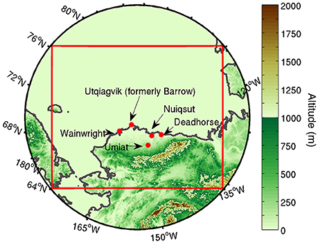
Figure 1. The WRF simulation domain (red box) with terrain heights (m). This downscaling product is specifically focused on the region of Arctic Coastal Plain and a small part of northern foothills of the Brooks Range with the domain enclosed by the red line.

Multiple observational and model-based studies have found that the Arctic sea ice has been declining since the 1970s. The sea-ice decline favors increased precipitation during the late fall and the early winter (Deser et al., 2010; Porter et al., 2012; Screen et al., 2013). Under the most extreme scenario in the Community Earth System Model (CESM) projection, the continuous Arctic sea ice decline eventually makes an ice-free September in the Arctic Ocean by the end of the 2040s (Wang and Overland, 2012). Projection under less extreme scenarios shows a declining rate of sea ice loss with sea ice minima remaining constant after the year 2070 (Bintanja and Van der Linden, 2013; Meehl et al., 2013). Such difference in sea ice extent may influence the seasonal cycles of air temperature and precipitation.

Polar Weather Research and Forecast Model

WRF is a flexible, state-of-the-art regional atmospheric modeling system (Skamarock et al., 2008). Previous modeling studies by polar MM5 (The Fifth-Generation Penn State/NCAR Mesoscale Model, with polar optimization) have emphasized the necessity of refining the parameters in surface background and physics schemes in terms of the Arctic regions (Cassano et al., 2001). We, therefore, employed the polar WRF (version 3.5.1), an Arctic-optimized WRF model plug-in, which was released by Polar Meteorology Group of the Byrd Polar and Climate Research Center at Ohio State University (Hines et al., 2009, 2011). Polar WRF model includes the upgraded physics schemes and revised land-use parameterizations specifically for both the terrestrial and oceanic Arctic (Hines et al., 2009; Wilson et al., 2011, 2012).

Forcing Datasets and Model Validation to Observations

ERA-interim reanalysis and Community Earth System Model version 1.0 (CESM1.0) output are used to force polar WRF in the period of 1979–2014. The historical WRF simulations (from 1950 to 2005) are forced by the CESM twentieth century all-forcing simulation output, while the future projections (the year 2006–2100) are informed by two scenarios of “Representative Concentration Pathways” (RCP4.5 and RCP8.5). Comparisons are conducted between the downscaled products (ERA-WRF), its forcing (ERA-interim), and the field observations (Global Historical Climatology Network Daily-summaries, GHCN-D). All products are bias-corrected based on the monthly climatology of ERA-interim.

ERA-Interim

ERA-interim, as the latest generation of reanalysis dataset by European Center for Medium-range Weather Forecast (ECMWF), serves atmospheric, land, and ocean elements in a T255 spectral resolution (roughly 80 km) globally (Dee et al., 2011). ERA-interim is made by models and data assimilation systems that ingest observations every 6–12 h (Dee et al., 2016). As an upgraded version of ERA-40, ERA-interim is empowered by Four-Dimensional Variational (4D-Var) data assimilation updated from the 3D-Var in ERA-40, making ERA-interim more observational-oriented (Lorenc and Rawlins, 2005; Whitaker et al., 2009). An improved representation of hydrological processes such as evaporation, condensation, and runoff has resulted in a refined accuracy of air temperature and moisture fields in ERA-interim (Dee et al., 2011). Most importantly, ERA-interim outperforms other reanalysis products in producing representative climatic variables over the high-latitudes (Jakobson et al., 2012; Lindsay et al., 2014).

Community Earth System Model 1.0

ESM-forced downscaling products are based on the CESM1.0 output. CESM is a group member of CMIP5 assembling the most advanced ESMs projecting the future global climate for the fifth Assessment Report (AR5) by International Panel on Climate Change (IPCC; Vertenstein et al., 2011; Taylor et al., 2012; Collins et al., 2013). One twentieth century all-forcing simulation (1950–2005) and two RCP scenarios (RCP4.5 and RCP8.5) for twenty-first-century projection (2006–2100) respectively forced Polar WRF. We chose the ensemble member of MOAR (“Mother of All Runs”). MOAR, represent the 12th member for the twentieth century, the 6th member for RCP4.5, and the 7th member for RCP8.5. MOAR is the only ensemble member that is with a 6-hourly output frequency, which is essential in building WRF boundary conditions. RCP projects a radiative forcing of 4.5 Wm⁻² for RCP4.5, and 8.5 Wm⁻² for RCP8.5 by prescribing the greenhouse gases emission increase in the twenty-first century. The RCP4.5 projects a mild global air temperature increase under stricter greenhouse gas control policies, while The RCP8.5 scenario prescribes uncontrolled greenhouse gas emissions and an extreme global warming (Moss et al., 2010; Riahi et al., 2011; Thomson et al., 2011). RCP8.5 helps to build the maximal global warming trend, while RCP4.5 fits closer to the observed global temperature change in the first decade of the twenty-first century, which has indicated a “braking” in global warming (Guemas et al., 2013).

Observation Data for Validation

North Slope of Alaska observation sites included in the GHCN-D observation data from National Climatic Data Center (NCDC) that are operating in the long-term mode are few. Five weather stations, Utqiagvik (formerly Barrow), Wainwright, Deadhorse, Nuiqsut, and Umiat, include daily precipitation and air temperature with <10% of missing data since 1980 (Figure 1). Here, we compared the GHCN-D monthly climatology of daily precipitation (PRCP), daily maximum temperature (TMAX), and daily minimum temperature (TMIN) to the ERA-interim dataset and ERA-WRF output, respectively. We present monthly climatology comparisons at Nuiqsut and Utqiagvik and are including other sites in the Supplemental Material. We bi-linearly interpolated ERA-interim variables and extracted WRF-outputs at the WRF grid point that was nearest to respective observation station. WRF's high resolution enables us to apply nearest neighbor interpolation method without generating unacceptable errors. In ERA-interim and WRF, the temperature record at 00:00 UTC (3 pm local time) in four (ERA-interim, 6-hourly) or eight (WRF, 3-hourly) records each day are defined as the TMAX, while the one at 12:00 UTC (3 am local time) as the TMIN. NCDC GHCN-D data records the maximum and minimum daily air temperature, while ERA-WRF and ERA-interim do not. Therefore, biases may inevitably arise during comparisons.

Model Initialization

The North Slope of Alaska is located in the center of the simulation domain, which covers part of the Beaufort Sea and the Chukchi Sea to the north, and Fairbanks to the south, forming a 180 × 150 gridded area with a 10 km horizontal grid spacing, that is, a 2.67 × 10⁶ km² of area (Figure 1). The temporal coverages are identical to the forcings, i.e., years 1979–2014 for ERA-WRF, 1950–2005 for the historical CESM-WRF, and 2006–2100 for the projected CESM-WRF. All runs started on July 1st in their first year of forcing. The first 6 months were the spin-up time and were excluded from the data analysis. We used the CESM output in a WRF intermediate file format downloaded from the Computational and Informational System Lab (CISL) Research Data Archive (ds316.0, no longer available online) to save computational time and expenses. Among the final downscaling products (Figure 2), CESM-WRF (historical and projected) offers climatic background based on the coarser-resolution GCM (CESM) output but with mesoscale dynamics and physics involved. On the other hand, the role of ERA-WRF is not only to offer a dynamically downscaled reanalysis dataset but also to validate the configuration of regional climate model (WRF in this case), as the climatic variables in it are directly comparable to observations. It is assumed that WRF simulates in the same manner forced by ERA-interim and CESM when with the same configuration (spatial/temporal resolution, time step of integration, parameterization of physics, etc.). Such workflow is commonly applied to dynamical downscaling projects, including NARCCAP and CORDEX (Giorgi et al., 2009; Mearns et al., 2013).

FIGURE 2

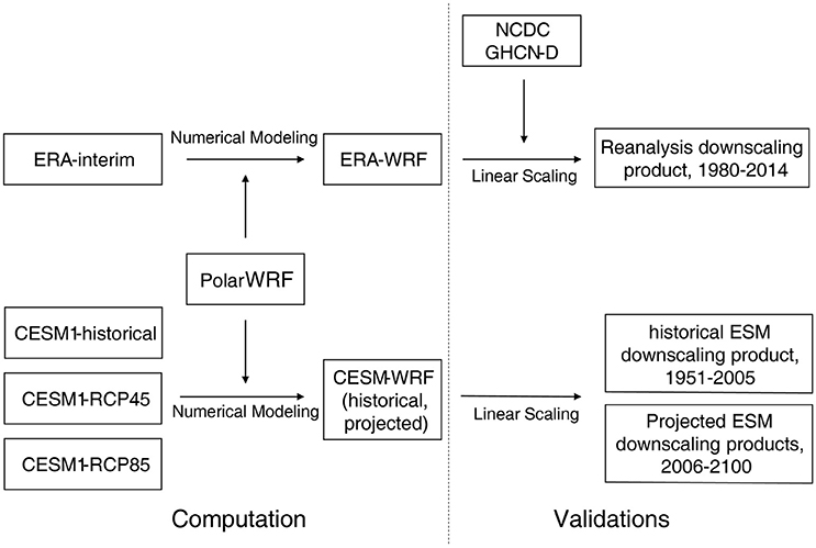
Figure 2. The flowchart indicating the steps involved in developing the three downscaling products.

Parameterization schemes were set to favor high-resolution, long-term runs. Multiple parameterization schemes were employed for various physical processes. For microphysics, WRF single-moment 5-class scheme (WSM5) was chosen (Hong et al., 1998). Rapid Radiation Transfer Model (RRTM) (Mlawer et al., 1997) and Dudhia scheme (Dudhia, 1996) were for parameterizing longwave and shortwave radiations, respectively. The Noah land surface scheme (Noilhan and Planton, 1989) was responsible for land surface processes, and the Yonsei University scheme (Hong and Dudhia, 2003) parameterized planetary boundary layer dynamics. Cumulus clouds were parameterized by the Kain-Fritsch convective scheme (Kain, 2004).

Multiple year-long test runs with different combinations of schemes were conducted before determining the combination of parameterization schemes. Double-moment microphysical parameterization schemes resulted in higher air temperature and precipitation biases in spring and early summer, which was caused by the overestimation of cloud formed, that reduced downward shortwave radiation at surface. We, therefore, turned to WSM5 scheme, a less advanced but more mature microphysical scheme that has shown more suitable for long-term modeling (Hong et al., 1998).

Nudging pulls values of key variables back to the forcing in a certain frequency in the entire simulation process, which helps to prevent model output deviating from the forcing (Glisan et al., 2013). However, while doing so, you also damage the physical correlation between the produced climatic variables, bringing higher uncertainty to the final product (Radu et al., 2008; Liu et al., 2012; Bullock et al., 2014). Data assimilation has the similar effect as it imports external data source into the modeling process (Fujita et al., 2007). We did not include any nudging or data assimilation during the computation in order to keep the full dynamical framework of WRF model intact and to allow the output variables to be physically correlated. Instead, to address any biases we adjusted model outputs by comparing results to observations after all computation was completed.

Bias Correction

The WRF simulation in this study inherits the biases from its forcings (i.e., ERA-interim and CESM outputs) as no nudging was involved in the downscaling process; therefore bias correction was applied to the WRF output. We utilized the linear scaling method for correcting the biases by rescaling the Probability Density Functions (PDFs), fitting the modeled monthly climatology to its reference (Lenderink et al., 2007; Teutschbein and Seibert, 2012). We employed a relatively simplistic bias correction approach in order to retain a majority of the sub-daily/daily variability in precipitation and air temperature while fitting the long-term climatology to the reference.

Two sets of bias-correction formulas resulted from two different PDFs distributions that precipitation and air temperature respectively hold. Climatologically, temperature PDFs generally obey normal distributions, while daily precipitation PDFs generally obey two-parameter gamma distributions (Harmel et al., 2002; Hanson and Vogel, 2008). The formulas for precipitation are represented by:

\begin{array}{rcl} P_{h i s}^{*} (d) = P_{h i s} (d) \frac{μ_{m} (P_{r e f} (d))}{μ_{m} (P_{h i s} (d))}, & (1) \end{array}

\begin{array}{rcl} P_{p r j}^{*} (d) = P_{p r j} (d) \frac{μ_{m} (P_{r e f} (d))}{μ_{m} (P_{h i s} (d))}, & (2) \end{array}

in which $P_{h i s}^{*} (d)$ and $P_{p r j}^{*} (d)$ are daily bias-corrected historical and projected precipitation, respectively, P_his(d) and P_prj(d) are the originals, and P_ref(d) is the daily reference precipitation. d is the notation standing for a certain day (data point), while μ_m stands for the function calculating the monthly climatology.

The formulas for air temperature follow as:

\begin{array}{rcl} T_{h i s}^{*} (d) = T_{h i s} (d) + μ_{m} (T_{r e f} (d)) - μ_{m} (T_{h i s} (d)), & (3) \end{array}

\begin{array}{rcl} T_{p r j}^{*} (d) = T_{p r j} (d) + μ_{m} (T_{r e f} (d)) - μ_{m} (T_{h i s} (d)), & (4) \end{array}

where the terms represent the air temperature and are otherwise the same as in the precipitation correction equations. References for linear scaling are ERA-interim monthly precipitation and temperature climatology. We also correct the biases in variables of snow water equivalent, dew point temperature, wind speed, and surface pressure and include them in the released dataset. Details of bias correcting other variables are presented in the Supplemental Material.

We are working under the assumption that the bias in the means calculated over the base period in the projected fields will stay the same with time. This is a commonly used approach (Teutschbein and Seibert, 2012; Bruyère et al., 2014). Note that we are not applying any targeted techniques to adjust variability in the modeled fields to the observed. We did not use the bias-corrected version of CESM output in the WRF intermediate file format (CISL ds316.1, Bruyère et al., 2014) for downscaling. As mentioned above, we are using raw CESM output in the WRF intermediate format instead, and apply bias correction to WRF fields after the simulation. As a cautionary note, bias correction procedure applied to precipitation will slightly modify the projected trends in the corrected fields.

Variables of model outputs mentioned in this manuscript, both before and after bias correction, are available through IARC data archive (http://data.iarc.uaf.edu/) and PANGAEA (https://doi.pangaea.de/10.1594/PANGAEA.863625). Other variables are also available upon request by contacting Lei Cai (lcai4@alaska.edu) or Vladimir Alexeev (valexeev@alaska.edu).

Results

ERA-WRF Evaluation

Our downscaling products are developed primarily for the North Slope of Alaska, while the area for evaluating them is extended until the South of the Brooks Range for a broader picture of performance. The downscaled ERA-WRF precipitation and air temperature climatology illustrate similar overall spatial distributions as its forcing, ERA-interim reanalysis data (Figure 3). However, the higher spatial resolution allows ERA-WRF to represent more detailed topographic features than ERA-interim. Differences include a higher amount of precipitation to the south and lower amount to the north in ERA-WRF compared to ERA-interim (Figures 3A,C). The ERA-WRF air temperature in the mountain regions is distributed following the topography, with colder areas coinciding with mountain peaks in the eastern Brooks Range where the altitude is higher than 1,500 m (Figure 3D). To the north of the Brooks Range, the ERA-WRF generally produces a drier (60–120 mm/year for precipitation) and a colder (2–3°C lower mean annual air temperature) climatology compared to ERA-interim. At the northernmost site (Utqiagvik), the annual air temperature bias reaches its maximum (up to 4°C colder in ERA-WRF compared to ERA-interim), while the precipitation bias reaches +60 mm/year. Warm biases (up to 2°C) are constrained to the mountain region mean annual air temperature (altitudes from 500 to 1,500 m). A section across the Brooks Range (red dashed line in Figure 3A) unveils a detailed view of the enhanced topographic effect to the more detailed terrain in WRF (Figures 3E–G). Precipitation and temperature in ERA-interim are monotonically decreasing toward North. ERA-WRF, however, presents double the annual precipitation amount of ERA-interim's (1,200 vs. 600 mm/year) on the south slope of the Brooks Range (Figure 3E). ERA-WRF also presents local minima of annual mean temperature on the mountain peaks (Figure 3F). An even higher variability of precipitation and temperature following the topography is presented by a 2-km resolution statistically downscaled dataset from Scenarios Network for Alaska and Arctic Planning (SNAP, 2017). However, there is no easy way to directly compare high resolution of SNAP dataset with observations or WRF-generated output. The mismatch between the real and model topography (or in this case SNAP topography) and lack of high-quality observations are the two main reasons why such comparisons should be done with a great deal of caution.

FIGURE 3

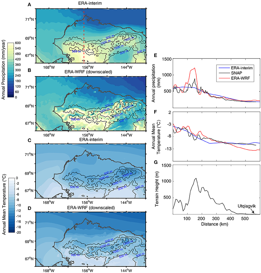
Figure 3. Original (ERA-interim) and downscaled (ERA-WRF) climatology 1980–2015 and elevation contour lines (black lines). Coarse resolution ERA-interim annual precipitation (A) and air temperature (C) compared to downscaled results from the ERA-WRF approach (B,D). Elevation contour lines in all figures are made from terrain height data in WRF. The annual precipitation (E) and mean temperature (F) distributions on the cross section (red dashed line in A) from ERA-interim (blue solid lines), SNAP (black solid lines), and ERA-WRF (red solid lines) show how a more detailed topography in ERA-WRF (G) affects the precipitation and temperature distributions.

Comparison to Observations

Monthly climatology comparisons to observations at Nuiqsut and Utqiagvik show that both modeled datasets (ERA-WRF and ERA-interim) present similar seasonal variability in precipitation, TMAX, and TMIN as the NCDC GHCN-D observations (Figure 4). However, modeled precipitation (ERA-WRF and ERA-interim products) consistently exceeds observations, while air temperature differences are more complex.

FIGURE 4

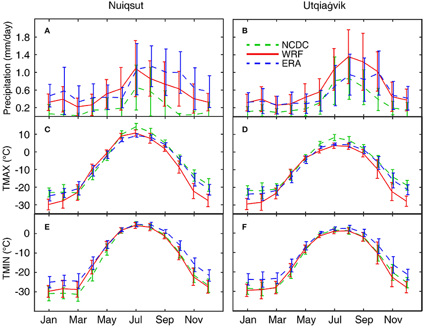
Figure 4. Monthly climatology comparisons between the NCDC GHCN-D observations (green dashed lines), downscaled ERA-WRF output (red solid lines), and ERA-interim reanalysis data (blue dashed lines) of average precipitation (mm/day), maximum and minimum air temperature (TMAX and TMIN, °C) for each month at the coastal towns of Nuiqsut (A,C,E) and Barrow (B,D,F). Average annual precipitation for these two stations is larger in the ERA-interim (215.4 mm) and the downscaled ERA-WRF (212.5 mm) than conventional observations (94.8 mm).

Dry biases occur mainly during October to February when ERA-WRF produces 30–50% less precipitation than ERA-interim at Nuiqsut (Figure 4A). The ERA-WRF wet bias compared to ERA-interim mostly results from higher April to October precipitation at Utqiagvik. The wet bias reaches +30% in the months of August and September. For the rest of the year, ERA-WRF and ERA-interim have nearly the same amount of monthly precipitation (Figure 4B). ERA-WRF and ERA-interim consistently produce 50–150% more precipitation than observations at Nuiqsut and Utqiagvik. Differences to observations are largest during the colder months (October to March) with 70 to 120 mm more precipitation than observed. As an example, total precipitation climatology (1980–2014) observed October to March was 7.8 and 32.1 mm (Nuiqsuit and, respectively), while ERA-WRF and ERA-Interim suggested 110.4 and 70.8 mm, as well as 132 and 84.3 mm for Nuiqsut and Utqiagvik respectively.

Correlation coefficients of monthly observed precipitation, TMAX, and TMIN are calculated in all five weather stations to both ERA-WRF and ERA-Interim after removing the seasonal cycles (Figure 5). The results indicate that the modeled time series of precipitation is correlated to observations. Correlation coefficients of both ERA-WRF and ERA-interim precipitation to observations are around 0.5 (>0.49 for 95% significance level) in most cases. Precipitation from ERA-WRF is more closely correlated to observations than ERA-interim at four out of five stations. Normalized standard deviations (SDs) of ERA-WRF and ERA-interim precipitation are larger than 1 in all cases except for ERA-interim precipitation at Wainwright. Such higher SDs indicate that the daily precipitation in both ERA-WRF and ERA-interim are with higher day-to-day variations than observation is, which typically the result of heavier rainfall events in ERA-WRF and ERA-Interim.

FIGURE 5

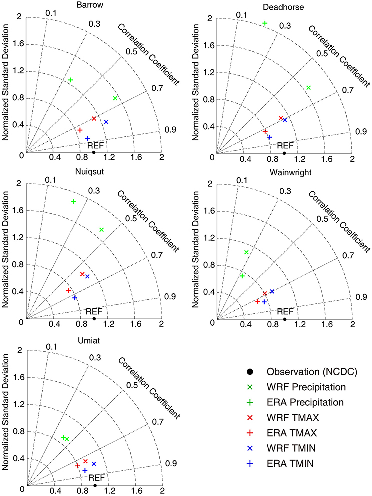
Figure 5. Taylor diagram with correlation coefficients and normalized standard deviations. The baseline values are NCDC GHCN-D observations (black reference dot). Shown are daily precipitation (green), daily maximum temperature (TMAX, red), and daily minimum temperature (TMIN, blue) in ERA-interim (ERA) and downscaled ERA-WRF (WRF) products. The annual cycles of each variable have been removed before calculating the correlation coefficients and standard deviations.

ERA-WRF simulates cooler TMAX than the observed in all months except for April and May at both Nuiqsut and Utqiagvik (Figures 4C,D). The TMAX difference averages up to 5°C in summer (July to August) and 8°C in winter (October to March). For TMIN, ERA-WRF produces a slightly warmer (<3°C) monthly TMIN than observation from January to May at Nuiqsut, while TMIN is almost identical for other months (Figure 4E). This is in contrast to the ERA-WRF TMIN results at Utqiagvik that are colder in winter than observations (<1°C in January to October and 2°C in November and December) (Figure 4F). The biases of ERA-WRF TMIN to observation at Utqiagvik are negligible in other months.

Diurnal temperature variations in both ERA-WRF and ERA-interim almost disappear in months from November to February. In these months, differences of TMAX and TMIN (TMAX minus TMIN) in ERA-WRF and ERA-interim are <1°C, while the GHCN-D observations show 5–8°C diurnal air temperature variation.

Daily TMAX and TMIN in ERA-WRF and ERA-interim are more correlated to observations than daily precipitation. Correlation coefficients for TMAX and TMIN are between 0.7 and 0.8 in all cases, which shows the significance of correlation and is 0.2–0.4 higher than the correlation coefficients for precipitation (Figure 5). Typically, TMIN in both ERA-WRF and ERA-interim are more correlated to observations than TMAX. In all stations except Wainwright, ERA-WRF produces TMAX and TMIN with higher variability than the observations (120% on SDs) and ERA-interim. ERA-interim produces TMAX and TMIN that are around 80% of SDs from observations at all five stations.

Statistics on Bias Correction

The cumulative probability functions of daily precipitation and mean air temperature in ERA-WRF and CESM-WRF historical products are changed after the bias correction (Figure 6). Compared to the model reference dataset (ERA-interim), the non-bias-adjusted ERA-WRF has more records (days) with no precipitation (<0.1 mm/day) or with light drizzles (<1 mm/day). On the contrary, the original CESM-WRF historical product shows a wet bias compared to ERA-interim. CESM-WRF has fewer days with no precipitation or light drizzles compared to ERA-interim, but more heavy precipitation events (>8 mm/day) (Figure 6A). The daily precipitation biases from ERA-WRF and CESM-WRF are adjusted via a 4.9% increase for ERA-WRF and a 30% decrease for CESM-WRF on respective long-term means based upon the climatology in ERA-interim. Both of the downscaling products also show decreased variances by 19% (ERA-WRF) and 47% (CESM-WRF) after correcting the biases. Showing on the cumulative probability curves, CESM-WRF precipitation closely fits the reference (ERA-interim) after the bias correction, while the biases in ERA-WRF precipitation are not corrected effectively on the drizzle side (<1 mm/day).

FIGURE 6

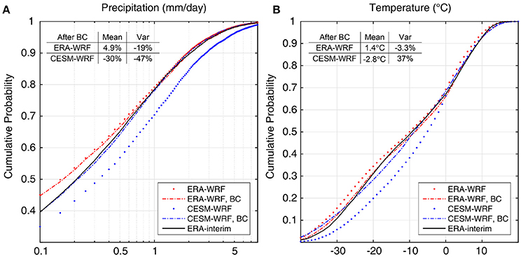
Figure 6. The comparisons of cumulative probabilities of (A) daily precipitation (mm/day) and (B) air temperature (°C) over coastal and foothill domain. Products are from the downscaled ERA-WRF (red dots), bias-adjusted downscaled ERA-WRF (red dash-dot lines), downscaled CESM-WRF historical product (blue dots), and bias-adjusted downscaled CESM-WRF historical product (blue dash-dot lines). The reference is represented by ERA-interim (black solid lines). Changes in the mean value and variance after bias adjustments are in percentage, except for mean air temperature that shows absolute changes in °C. Linear scaling adjusts biases more effectively in precipitation than in air temperature, and more so in CESM-WRF compared to ERA-WRF.

Generally, the linear scaling corrects precipitation more than air temperature. For daily air temperature, the cold bias in ERA-WRF and warm bias in CESM-WRF are corrected with a 1.4°C and a −2.8°C changes, respectively (Figure 6B). The historical CESM-WRF simulates a warm bias in air temperature, also it underestimates seasonal cycle. Applying monthly seasonal bias correction leads to a 37% increase in seasonal variability in CESM-WRF. A similar bias correction applied to ERA-WRF results in a slight decrease (−3.3%) in the seasonal cycle of air temperature.

CESM-WRF received larger bias-corrections on both daily precipitation and air temperature compared to ERA-WRF. The bias correction on CESM-WRF produces more days with light drizzles and cold air temperatures (temperature <0°C) due to its original warm and wet biases. The bias corrections on ERA-WRF addressed mostly its cold and dry biases.

CESM-WRF Projection

All estimates presented in this section are averages for the whole domain of the North Slope as defined in section Site Description. All three CESM-WRF products exhibit increasing trends in annual precipitation and air temperature (Figures 7A,B). Precipitation from CESM-WRF RCP8.5 has the largest increasing trend (nearly +1 mm/year), resulting in an annual precipitation of nearly 500 mm by the end of the twenty-first century compared to 400 mm at present. In comparison, the annual precipitation in the historical and the RCP4.5 products increase only 0.62 and 0.36 mm/year, respectively. The RCP8.5 projection has also the largest increasing trend of annual mean temperature. The RCP4.5 projection, on the other hand, presents an increasing trend of precipitation that is smaller than the historical simulation. By the end of twenty-first century, the North Slope of Alaska experiences a 5°C warmer annual mean air temperature in RCP8.5 compared to the RCP4.5 scenario (8.5° vs. 3.5°C, respectively). The historical simulation (from 1950 to 2005) shows a 3.1°C air temperature rise.

FIGURE 7

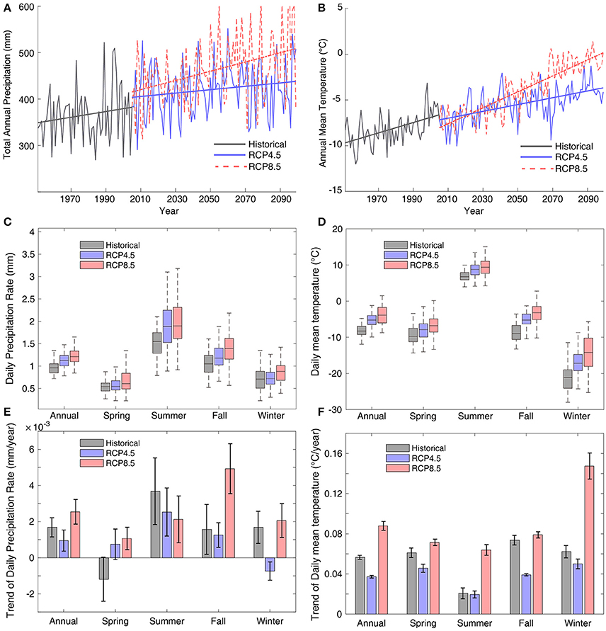
Figure 7. The time series of (A) total annual precipitation and (B) annual mean air temperature. Represented are the historical (gray), RCP4.5 (blue), and RCP8.5 (red) downscaling products. Box plots show the annual and seasonal (C) daily precipitation rate (mm) and (D) daily mean air temperature (°C) from the three downscaling products, annual and seasonal trends of (E) daily precipitation rate (mm/year), and (F) daily mean temperature (°C/year).

In order to compare the annual and the seasonal trends of precipitation, we calculated both the precipitation amounts and trends based on the daily precipitation rate (mm per day). All three products (CESM-WRF historical, RCP4.5, and RCP8.5) produced the most precipitation in summer (JJA, 1.5–2 mm/day on average) and least in winter (DJF, 0.6–0.8 mm/day on average) (Figure 7C). Higher annual and seasonal precipitation amounts are found in the twenty-first-century projections compared to the historical precipitation. The RCP8.5 projection has more precipitation than the RCP4.5. The summer (JJA) is also found with the largest increasing trends of precipitation in the historical (0.004 mm/day per year) and RCP4.5 products. For the RCP8.5, however, the largest increasing trend of daily precipitation rate is in fall (0.005 mm/day per year). In winter, RCP8.5 precipitation also increases rapidly (over 0.002 mm/day per year). Trends in winter precipitation in the historical and the RCP4.5 (0.002 and −0.001 mm/day per year) are substantially smaller than summer (0.004 and 0.003 mm/day per year).

Both the RCP4.5 and the RCP8.5 projections produce increases in air temperature in all four seasons. Increases in winter air temperature are largest (Figure 7D). RCP8.5 results in an air temperature increase of 0.15°C/year during winter, which is more than in any other season (from 0.06 to 0.08°C/year). Similar, albeit not as large, seasonal trends are found in the RCP4.5 scenario. The larger warming in winter than summer implies a reduced seasonal variation of air temperature in the twenty-first-century projections.

Discussion

Dynamical downscaling by the Polar WRF model presents refined climate products in regards to spatial and temporal distributions of precipitation and air temperature for the North Slope of Alaska. The coarse (roughly 80 km) grid spacing of ERA-interim is not sufficient to effectively represent the topographical effects in air temperature and precipitation. Such a coarse resolution underestimates the complexity of topography in Arctic Alaska; for example, the highest peak of the Brooks Range has the elevation of 1,836 meters in WRF while the same peak is only 1,070 meters in ERA-interim. Such enhancement of topography in WRF is important for our area of interest, the North Slope of Alaska, for which the Brooks Range plays an important role in its regional climate. The Brooks Range in WRF obstructs more of the warm and wet air from reaching the North Slope of Alaska than in ERA-interim. Although such enhancements due to the topographical effect cannot be precisely quantified from the ERA-WRF simulations, it is clear that the more detailed topography in ERA-WRF results in higher precipitation and temperature on the southwest side, while lower ones on the north side, of the Brooks Range, compared to ERA-interim (Figure 3). The warmer winter temperatures in the mountainous area of the Brooks Range at 500–1,500 meters altitude are likely to result from the enhanced vertical resolution in the atmosphere interacting with micro-topography in ERA-WRF that causes stronger modeled inversions in valleys.

Both ERA-WRF and ERA-interim produce more than double the amount of winter precipitation compared to available observations. Conventional snowfall observations are known to have issues with underestimation and accuracy in general (Groisman and Rankova, 2001; Bogdanova et al., 2002; Groisman et al., 2004), making quantitative analysis difficult. Differences between modeled and observed precipitation in this study are comparable (100~400 %) to the assessments done by Liljedahl et al. (2017), which compared conventional snowfall measurements to end-of-winter snow accumulation near Utqiagvik, Alaska. In summary, our downscaled annual mean precipitation is likely to be more realistic than that derived from ERA-interim or CESM.

Evaluation experiments by the Polar WRF group found a cold bias in winter on the North Slope starting with Polar WRF version 3.1.1 (Hines et al., 2009, 2011). As we found here, the winter cold bias remains in polar WRF version 3.5.1. ERA-WRF produces smaller biases in TMIN (−1 to −3°C) than in TMAX (−5 to −8°C) when compared to observation. Hines et al. (2011) discovered that polar WRF overestimates downwelling longwave radiation (cloudier days and nights) while underestimating wind speed from January to March in Barrow in the test simulations, with both factors contributing to the decrease in the wintertime diurnal temperature variation in Arctic Alaska. Tuning of cloud and longwave radiation schemes may help reduce such biases slightly, while further significant improvements in reproducing diurnal cycle of temperature in winter depending on the upgrades of polar WRF itself. The applications for which our downscaled products have been developed primarily utilize data in the type of daily/monthly means instead of diurnal extremes so that the impacts of such deficiencies have been minor. Improving the diurnal cycle in WRF in cold season should become one of the priorities that will help model the winter on the North Slope better.

The historical CESM-WRF generally simulates a wet bias in precipitation and a warm bias in air temperature compared to ERA-interim. Most biases in CESM-WRF resulted from biases in CESM. CESM1.0 historical product evaluation found warm biases on air temperature and wet biases on precipitation compared to ERA-interim over the Northern Alaska and the Beaufort and the Chukchi Seas to the North, and the maximum warm (+5°C) and wet biases (+100%) are both present in winter, similar to de Boer et al. (2012). CESM-WRF in this study retains at least part of such deficiencies of CESM, having higher precipitation and air temperature biases than ERA-WRF in the historical period. de Boer et al. (2012) also unveiled the deficiency of CESM1.0 in underestimating total cloud fraction all year round over the Arctic Alaska compared to observation. CESM-WRF in this study has improved performance in retrieving cloud cover over CESM due to higher spatial resolution and more complex physics schemes. Walston et al. (2014) found that CESM1.0 underestimates the seasonal cycle of air temperature over the Arctic through warmer winters and colder summers compared to reanalysis data. The similar seasonal variability is muted in our CESM-WRF simulations, which is partially improved by the bias-correction that imports the ERA-interim seasonal cycles.

Downscaled projections forced by RCP4.5 produced a lower increase in the annual total precipitation (+0.36 mm per year) than the historical product (+0.62 mm per year). RCP8.5– informed projections show the largest trend (+0.99 mm per year). Almost half of the precipitation increase in RCP8.5 occurs in October through December. The large increase in fall precipitation may be attributed to the rapid sea ice decline in the CESM RCP8.5 product (Alexeev et al., 2016). CESM-WRF historical product presents larger positive trends of precipitation and air temperature than the RCP4.5 projection. We attribute it to the choice of years we set as the historical period (1950–2005), which coincides with the strongest climate change during the whole historical simulation period of CMIP5 models (1850–2005). On the contrary, the RCP4.5 scenario features a stabilization of global warming, so that the global mean temperature increase slows down after 2060, which is reflected on all CMIP5 models (Collins et al., 2013). Since our projected trends are calculated for the period of 2006–2100, such “deceleration” of global warming after 2060 in RCP4.5 scenario lowers the overall increasing trend. Specifically for the Arctic Alaska, the sea ice decline in RCP4.5 scenario also slows down after 2050 to a rate that is lower than our historical period (1950–2005) (Stroeve et al., 2012). Such changes in sea ice also inhibit the increase of precipitation and air temperature, primarily in late fall and early winter (Stroeve et al., 2007).

We did not address comparisons between the projected CESM-WRF and the original low-resolution CESM RCP projections as such analysis is less informative because the applied bias correction procedure inevitably brings artifacts to climatic variables. While the boundary forcing for WRF can come from different products (ERA-Interim or CESM), the dynamics and physics in the interior of the domain (North Slope of Alaska in this case) are determined entirely by WRF. The downscaling of ERA-interim, CESM historical products, and CESM future projections is done in this study under an identical setting (spatial/temporal resolutions, integrating time step, physics schemes, etc.). Our ERA-WRF evaluation comparing with ERA-interim and observations have demonstrated the role of WRF and its configurations in improving the quality of fields by applying the dynamical downscaling over the North Slope of Alaska. We argue that our CESM-WRF products have more realistic mesoscale features and therefore are superior compared to the original CESM output (historical and projected) including the effects of enhanced topography and more extreme precipitation.

Our downscaling data products present high spatial grid spacing (10 km), long temporal coverage (1950–2100), high-frequency output (every 3 h) and are the only multi-scenario climate projections (RCP4.5 and RCP8.5) for the Arctic Alaska. Without any nudging or data assimilation, the ERA-WRF and CESM-WRF products for the historical period have higher biases compared to observations than the datasets developed by Bieniek et al. (2016) and Zhang et al. (2016). Here, we deal with these biases by applying linear scaling bias corrections, which resulted in biases being corrected toward the ERA-interim reanalysis dataset. The historical ERA-WRF and CESM-WRF climate products combined with future warming scenarios (RCP4.5 and 8.5) make our dataset particularly suitable for the regional climate change studies over the North Slope of Alaska.

Conclusions

This paper introduces a set of dynamical downscaling products forced by both ERA-interim reanalysis data and CESM model output. The model evaluation shows that the dynamical downscaling process resolves more detailed topographical effects on the regional climate of the North Slope of Alaska compared to its forcing datasets. The higher resolution surface topography in WRF (compared to the low-resolution topography in ERA-Interim and CESM) helps reproduce more reasonable climate background in Arctic Alaska that has a complex terrain. The modeled annual mean precipitation is 100–400% higher compared to observations, the reasons for which are highly debatable, including the lack of high quality observed precipitation datasets in the high Arctic. The WRF-modeled precipitation also increases seasonal variability compared to the original forcing products. We view the dynamical downscaling as a valid approach to producing not only more realistic long-term mean products, but also more extreme events that can only be represented in the mesoscale framework. The two downscaled products that project the twenty-first-century regional climate agree on a trend toward a warmer and wetter North Slope of Alaska. The RCP4.5 simulation exhibits a smaller increasing trend in precipitation and air temperature compared to the RCP8.5 products. The projected increases by RCP4.5 are even lower than that of the historical product. Trends are largest in fall and winter in the RCP8.5 projections. More detailed study on the CESM-modeled sea ice decline impacts may help to explain such differences. The downscaled data products of high-resolution, long temporal coverage and multi-scenario future projections have the potential to refine climate change studies over the North Slope of Alaska and ultimately resulting in more effective impact assessments for the people living in the region due to the finer spatial and temporal scales and improved representation of extreme events.

Author Contributions

LC: develop the dataset, do data analysis, and draft the manuscript. VA, CA, BJ, and AL: set the design of the work, give critical ideas and revision comments on data analysis and manuscript writing. AG: help on dataset development and data analysis, give critical revision comments.

Conflict of Interest Statement

The authors declare that the research was conducted in the absence of any commercial or financial relationships that could be construed as a potential conflict of interest.

Acknowledgments

Funding for this research is provided by National Science Foundation (ARC-1107481 and ARC-1417300) and the Arctic Landscape Conservation Cooperative. We thank Andrew Monaghan for converting and sharing CESM data in a WRF intermediate data format. We thank Benjamin Gaglioti for proofreading and helpful comments on polishing the language. Any use of trade, product, or firm names is for descriptive purposes only and does not imply endorsement by the U.S. Government.

Supplementary Material

The Supplementary Material for this article can be found online at: https://www.frontiersin.org/articles/10.3389/feart.2017.00111/full#supplementary-material

References

Alexeev, V. A., Arp, C. D., Jones, B. M., and Cai, L. (2016). Arctic sea ice decline contributes to thinning lake ice trend in northern Alaska. Environ. Res. Lett. 11:074022. doi: 10.1088/1748-9326/11/7/074022

ORIGINAL RESEARCH article

The Polar WRF Downscaled Historical and Projected Twenty-First Century Climate for the Coast and Foothills of Arctic Alaska

Introduction

Methodology

Site Description

Polar Weather Research and Forecast Model

Forcing Datasets and Model Validation to Observations

ERA-Interim

Community Earth System Model 1.0

Observation Data for Validation

Model Initialization

Bias Correction

Results

ERA-WRF Evaluation

Comparison to Observations

Statistics on Bias Correction

CESM-WRF Projection

Discussion

Conclusions

Author Contributions

Conflict of Interest Statement

Acknowledgments

Supplementary Material

References

People also looked at