Forecasting Summertime Surface Temperature and Precipitation in the Mexico City Metropolitan Area: Sensitivity of the WRF Model to Land Cover Changes

Introduction

Changes in frequency and intensity of extreme events of precipitation and heat waves (Jáuregui, 2000; Magaña et al., 2003; López-Bravo, 2012) have been accompanied by increases in the frequency and impact of weather-related disasters in Mexico City Metropolitan Area (MCMA) in recent decades. Although a weather forecasting system cannot prevent disasters, alert systems are vital for the authorities to take the necessary measures and thereby mitigate the effects of hydrometeorological extreme events. Therefore, accuracy in weather prediction is important if decision-makers are to protect life and property and improve socio-economic well-being and the environment.

Studies of temperature, humidity, wind, and precipitation in MCMA have investigated the dynamics of meteorological events such as heat waves, extreme precipitation, and storms (Aquino, 2012; López-Bravo, 2012). Since this is the most populated region of the country, with 20 million inhabitants (INEGI, 2010), the meteorological phenomena affect millions of people. Additionally, accelerated urban growth since the 1970s and changes in land cover have caused alterations in atmospheric conditions, giving arise to a heat-island climate (Jáuregui, 2000; López-Bravo, 2015). Urbanization has affected the small-scale atmospheric circulations that are induced by differential heating, thereby modifying the structure of the planetary boundary layer, forming convergence zones, and changing stability conditions with repercussions on air quality. These changed conditions act as forcings in the generation of severe weather, especially in the formation and increasing development of convective storms (Jáuregui and Romales, 1996; Jáuregui, 2000). During the last century, the frequency of rainfall events <30 mm in 24 h increased from 10 to 25 events per decade (Jáuregui and Romales, 1996), and extreme events of >20 mm/h (Figure 1) increased by an order of magnitude (Jáuregui, 2000).

FIGURE 1

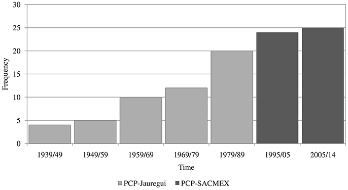
Figure 1. Frequency of intense precipitation events > 20 mm/h from July to September, during 1939–1989 (Jáuregui, 2000) and 1995–2014 SACMEX station.

Although many numerical forecasting systems have been implemented in Mexico, most of them have no verification schemes to generate trustworthy information for users. For example, there are sources of error in the local circulation associated with the orography or the interaction of the mean moist flow from the Gulf of Mexico with the mountain barriers near MCMA. The rainfall, 2 m, and surface temperature predictability depends on the flow and energy interaction between different scales of motion and it is sensitive to the amount of energy described in the initial condition (Slingo and Palmer, 2011). In mesoscale models, surface inhomogeneities resulting from a rough description of terrain and/or surface features (albedo, soil heat capacity, available moisture, etc.) generate dynamic processes that are inadequately represented (waves generated by interaction of flow with mountain barriers, convection, mountain-valley breezes, orographic precipitation, etc.; Mölders, 2011). Hence, it is necessary to describe adequately the surface forcing, making an appropriate choice of surface characteristic parameters and physical processes parametrizations to capture mesoscale phenomena in high-resolution models (Ray, 1986).

This study examines the causes of errors, associated to land cover changes and initial boundary condition, in the numerical forecasting for MCMA, specifically in the accumulated precipitation at 24 h to improve the predictability of the Weather Research and Forecasting Model (WRF).

Data and Methods

Gridded Observation Data Set

Hourly and daily gridded observation data sets were created from meteorological data across Mexico provided by the National Water Commission and the Watershed Organization (642 stations nationwide). Radiosonde observations (00:00 and 12:00 UTC) were obtained from the National Oceanic and Atmospheric Administration (NOAA). The North American Regional Reanalysis (NARR) (Mesinger et al., 2006) was used as the first-guess field to construct a regularly gridded data. After performing the quality control (Klein Tank et al., 2002) for climatological and automatic stations and rain gauges. The station data were carried out a statistical analysis with the objective of determining the quality of the information. Three standard deviations and threshold values of percentiles were used for the analysis of extreme values in order to assess the consistency and coherence of the information. The data were interpolated to regular meshes using an objective analysis scheme based on successive corrections (Cressman, 1959). The first step in this process is to combine the observations and a first-guess field. After a first pass is made through the domain, consecutive passes are made, modifying the field at each grid point based on the observations surrounding the grid point regarding a radius of influence. In all cases four iterations were made in each of the three developed databases. The radii of influence were: (a) for 4 × 4 km dataset (10, 8, 6, and 5 km); (b) for 5 × 5 km dataset (12, 10, 8, and 6 km) and; (c) for 10 × 10 km dataset (20, 15, 13, and 12 km). The weight factor was calculated with the inverse of the square of the distance. This radius of influence is usually set to decrease for each pass through the field so that it is corrected from larger scale features during the first iterations to smaller scale features during latter iterations. For the gridded precipitation set, two climatological databases were constructed at different spatial and temporal resolutions: (1) the hourly 4 × 4 km grid for the period 2003–2013 constructed from the rain gauge network of the Water System of MCMA, and CMORPH (NOAA CPC MORPHing Technique, Joyce et al., 2004) precipitation estimates as first-guess; and (2) a daily precipitation dataset using climatological stations of the National Meteorological Service (SMN), and as first-guess the combination of NARR reanalysis and CMORPH satellite estimates, with a horizontal resolution of 10 × 10 km for the period 1979–2010. For the maximum and minimum daily temperatures from SMN, and as first-guess NARR reanalysis, two datasets with horizontal resolutions of 5 × 5 km and 10 × 10 km were also produced for the period 1986–2010. A temperature–height adjustment was applied as follows:

$\begin{array}{ll}tm{p}_c=tm{p}_{NARR}-{\Gamma }_d\Delta z.& (1)\end{array}$

This adjustment considers the height difference Δz between the topography described in NARR and the Scripps topography (Smith and Sandwell, 1997). The height difference determined the rate of change to adjust the temperature value (Figure 2) at each mesh point considering the standard lapse rate (Γ_d) of 6.5 K/km (Minder et al., 2010). The adjustment is made to the first-guess before performing the first iteration. The purpose is to improve the quality of the first-guess. After making the correction with the Cressman scheme, the information was validated against observations to determine the ability of the database to capture phenomena and their evolution on spatial scales of the order of tens or a few kilometers and on time scales of hours and days.

FIGURE 2

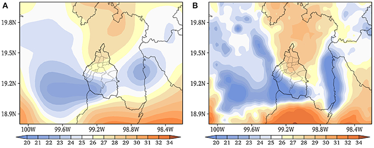
Figure 2. The 2 m temperature field (°C), Mexico City, from NARR (A), and calculated orographic adjustment (B).

Experiment Set-Up

The WRF model version 3.5 (Wang et al., 2014) was used in all experiments. Each run was initialized at 00:00, 06:00, and 12:00 UTC to 36-h simulation. The first 12 of 36 h forecast is left to the dynamic adjustment of the initial fields. A single domain with 12 km horizontal resolution and 36 vertical levels (with vertical levels stacked near the ground) was defined. The domain was centered on the southern state of Veracruz (Lat. 17.5°N, Lon. 95.0°W), covering a region ranging from 0 to 35°N and from 120 to 70°W (Figure 3). The initial and boundary conditions fields were obtained from the Global Forecast System (GFS) with a horizontal resolution of 0.5 × 0.5° and a temporal resolution of 3 h (National Centers for Environmental Prediction, National Weather Service, NOAA, 2015).

FIGURE 3

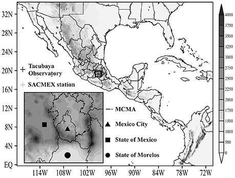
Figure 3. The domain used in WRF experiments. Topography in shaded (m).

The WRF Initialization

The regional modeling is a problem of initial and boundary conditions. After sensitivity tests in the design of domain and spatial resolution, the next step was to select the initialization method. The enhanced initial condition was obtained with the OBSGRID-WRF preprocessing module using the Cressman (1959) successive correction method for surface observations (Figures 4A,B) and radiosonde data (Figure 4C). The adjusted forecast variables were temperature, relative humidity, geopotential height, and the zonal and meridional winds. The capability of the scheme largely depends on the density of the data available for the region, the number of iterations, and the selected radius of influence. Two variants of empirical Four-Dimensional Data Assimilation (FDDA) were examined: the experimental observation nudging and analysis nudging (Stauffer et al., 1991; Stauffer and Seaman, 1994; Fast, 1995; Seaman et al., 1995; Liu et al., 2005). The initialization technique applies the FDDA cycling method to add observation data during the model spin-up period to examine the effect of dynamic initialization by applying large-scale analysis data. Observation-nudging assimilates all of the observation data from each hour in the adjustment period. The procedure used was a combining of grid-nudging and observation-nudging methods, called hybrid method (Yu et al., 2007).

FIGURE 4

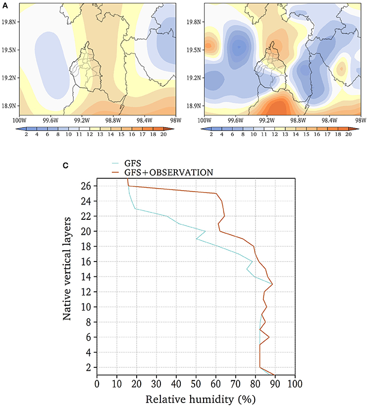
Figure 4. Comparison of the 2 m temperature field (°C) at 12:00 UTC 16 July 2014: (A) GFS model; (B) GFS model plus observations using Cressman objective analysis; and (C) the relative humidity profile (%) of the GFS model (blue line) and the GFS model plus radiosonde (brown line).

Results

Impact of Urban Area Extent

An analysis of the static model parameters is presented, owing to their importance in surface physics and their implications on the activation and feedback mechanisms involved in cloud formation and the microphysics of precipitation. The coverage and extension of the urban sprawl described in the geographic databases available in WRF does not quite agree with the actual urban sprawl areas in 2005 and 2010 as reported by INEGI (Figures 5A,B); consequently, the roughness, albedo, vegetation cover, and parameters related to the description of surface fluxes of moisture, heat, and momentum do not capture adequately the surface processes and the planetary boundary layer dynamics.

FIGURE 5

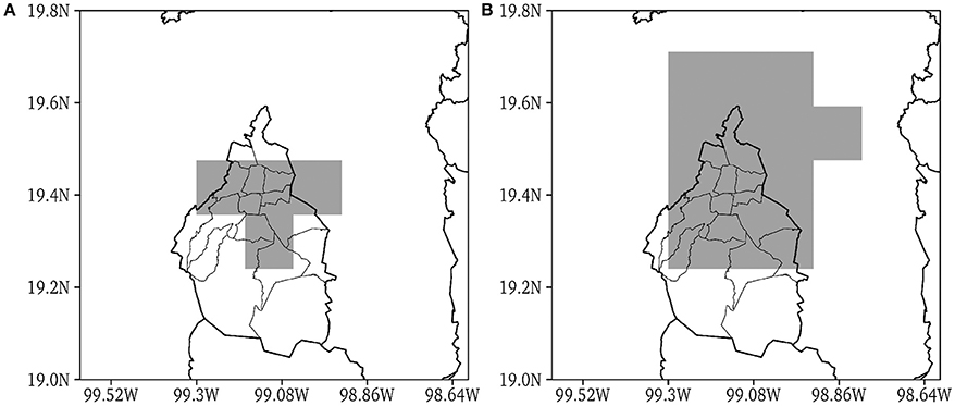
Figure 5. Spatial distribution of the urban area at 12 km horizontal resolution (A) from the WRF geographical database and (B) modified with INEGI data for 2005–2010.

Two experiments were performed over a period form 1 July to 31 July 2014 to quantify the impact of the land cover on the forecast: the first (control) experiment took land cover from the geographic data of the WPS Version 3.5.1, and the second experiment used an updated land cover and its associated parameters. Each experiment considered the Noah surface scheme (Chen et al., 1996; Chen and Dudhia, 2001; Ek et al., 2003) and the planetary boundary layer scheme developed by Yonsei University (Hong et al., 2006). The 2 m air temperature (tmp2m) and skin temperature were incorporated in the sensitivity analysis since they are associated with the energy transfer between the surface and the atmosphere. The experiments with different degrees of urbanization for a tmp2m forecast at 17:00 UTC showed average differences of 3°C over regions with significant land cover changes (north and east of MCMA, and the eastern part of the State of Mexico–Texcoco Lake). An inadequate description of the land cover generates spurious circulations, which are a source of errors in the estimates of the surface fluxes of heat, moisture, and momentum (Lee et al., 1989; Wolyn and McKee, 1989; Shafran et al., 2000; Cheng and Steenburgh, 2005) that affect the mechanisms of activation and development of mesoscale systems.

The WRF Skin Temperature

The simulation for 21 July 2014 reproduces quite well the skin temperature, compared with the observation derived from a Moderate Resolution Imaging Spectroradiometer (MODIS) with a spatial resolution of 1 × 1 km (Figure 6). The model has the ability to reproduce the spatial variation of skin temperature with respect to orography. However, it seems to overestimate the temperature over the urban sprawl by 2–4°C when compared with the MODIS estimates. This difference can be attributed to the WRF configuration used, where homogeneous urban cover considers only the mean values of albedo, emissivity, evapotranspiration, etc., and local heat and moisture sources and sinks. In some cases, there may be a factor inhibiting groundwater evaporation, or changes in temperature that could favor ventilation in the city (Mölders, 2011). Also, owing to the type of surface scheme used, strong thermal contrasts are established on the urban outskirts, changing the stability conditions of the region and causing artificial circulations that do not correspond to the observed patterns (this effect is discussed later). Over elevated regions, the vertical gradient tends to weaken compared to observation since the horizontal resolution (12 km) smoothes the complex topography. In general, the modified version tends to capture the distribution of the skin temperature in position and shape of the orographic component and the urban area, responding to urbanization as the main forcing.

FIGURE 6

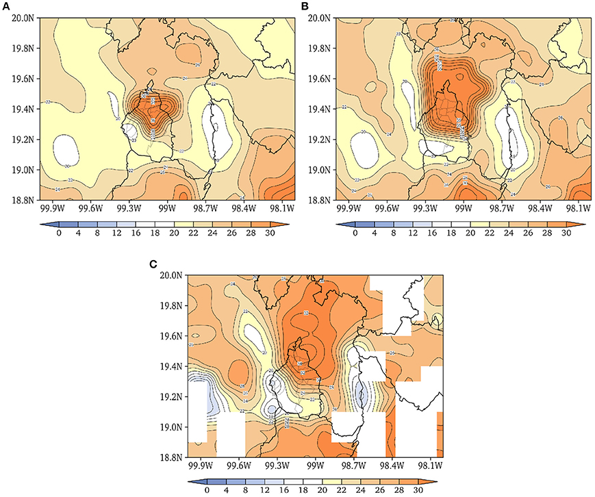
Figure 6. Comparison of skin temperature (°C) for 21 July 2014 between experiments: (A) Control experiment; (B) Experiment modifying land cover; and (C) MODIS satellite images.

Verification of 2 m Air Temperature

The error of tmp2m for July 2014 between the 24 h forecast and gridded observations is discussed below. The sites were selected for their characteristics (urban region, city outskirts, and sites where the orographic component is important).

According to the Taylor diagrams presented (Figure 7), the mean square error (RMS) in the temperature variable at 2 m presents a small improvement in the WRF-modified version, except in the case of the Madín dam. Through the scatterplot (Figure 7) the correspondence between the simulated field and the observed field is confirmed. Other inferences drawn from the Taylor diagrams can be confirmed in the scatterplot. For example, both versions of the control and modified model are correlated in a similar way with the observation (both with a value close to 0.8), although the control and the modified version are out phased respect to the perfect forecast line.

FIGURE 7

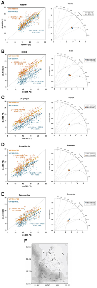
Figure 7. (Left) Hourly air temperature dispersion at 2 m (°C) in different regions of the MCMA (July 2014). Blue dots, WRF control; orange dots, modified WRF. Regression equations follow the same color scheme. (Right) The Taylor diagram (Taylor, 2001) (A) Tezontle, (B) ENCB, (C) Chapingo, (D) Presa Madín, (E) Ecoguardas, and (F) Location map for the analyzed points (A–E).

The Taylor diagrams provide much of the information presented in the scatterplot, but the sample in a way that allows to detect/show problems in a simplified way (Taylor, 2001).

Urban

The points selected within the urban sprawl contain the Tezontle and ENCB stations. The location of Tezontle (urban land cover) was considered as a reference site because in the control and the modified experiments the static parameters did not undergo significant changes (Figure 7A). In the case of the ENCB, it was possible to remove the systematic bias present in the control version. The modified version was nearly a perfect forecast where the predicted conditions approximated the observation. An increase in temperature of up to 4°C (Figure 7B) was attributable to the change in land cover.

Semi-urban

The Chapingo-Texcoco site is semi-urban; in recent years, accelerated urban development has affected temperature trends. In the results, the bias was removed, but the tilt of the scatterplot has changed, and there are problems in forecasting maximum values (Figure 7C). There is also a widening in the dispersion of the points toward high-temperature values. This error may have been induced by the resolution of the experiment, the new description of the land cover, and numerical effects associated with parametrization generated by solving the soil conditions with very contrasting properties, such as an urban region and an area with a different land cover type (Mölders, 2011; Sharma et al., 2017). In general, mesoscale models present systematic errors dependent on resolution and scale (very contrasting conditions at very small spatial scales) (Warner, 2010).

Orography

The temperature forecast at the Madín Dam at the foot of the Sierra de las Cruces (Figure 7D), and Ecoguardas on the slopes of the southern mountains of Mexico City (Figure 7E) show a significant improvement in simulation period (hourly) values, the bias was removed, and the modified version scatterplot was fitted to theoretical line of perfect forecast. Despite the improvement made, the ability to forecast extremes temperature is decreased. The reason might be that the mesoscale models have low prediction skill over complex terrain (Jiménez and Dudhia, 2013).

Valley-Mountain Circulation

The MCMA experiences two types of local circulations: those generated by mountain-slope winds and those generated by the local effect of the heat island. They are easier to identify when the large-scale flow is weak (Wang et al., 2015). The effect of urbanization on the thermal oscillation in the city has become smaller than in the non-urbanized regions (Oke, 1987). Diurnal variations in winds, temperature, and humidity also affect the efficiency of vertical mixing in the planetary boundary layer. The MCMA mixing layer is deeper than in neighboring regions, and this causes strong convergence at low levels over the city. Bearing in mind the importance of the diurnal cycle in modeling mesoscale systems (e.g., genesis and evolution of storms), the ability of WRF to simulate the mountain–valley circulation within Mexico City was assessed. On 31 July 2014, a weak synoptic condition was present, and a local forcing circulation was dominant over the region. The evolution of the diurnal cycle in the valley–mountain circulation was fairly well reproduced by WRF. During the first hours of the day a valley breeze upslope flow is established (Figure 8A), when the heat transfer processes between the city and the elevated zones become more efficient. The inversion of the wind direction occurs toward the evening hours (Figure 8B) when the dominant winds of the day begin to lose strength. The change of direction and magnitude of the wind is gradual, with a decrease in the temperature gradient resulting from mechanisms of horizontal advection of temperature and release of sensible heat. Once the inversion has occurred, the mountain valley winds flow downslope transporting more “cold” air to the city center. The configuration of the mountains surrounding Mexico City, especially to the west and the south (Figure 3), determine the circulation patterns. During the descending mountain flow, a surface convergence is generated in the middle of MCMA. The heating throughout the day is characterized by a thermal gradient between the city and the elevated region, reaching a maximum temperature between 17:00 and 22:00 UTC. The change of temperature toward the afternoon shows a low efficiency to emit the energy retained throughout the day, and this keeps the warm air near the surface. In contrast, the elevated region emits energy more efficiently, and the temperature decreases more quickly.

FIGURE 8

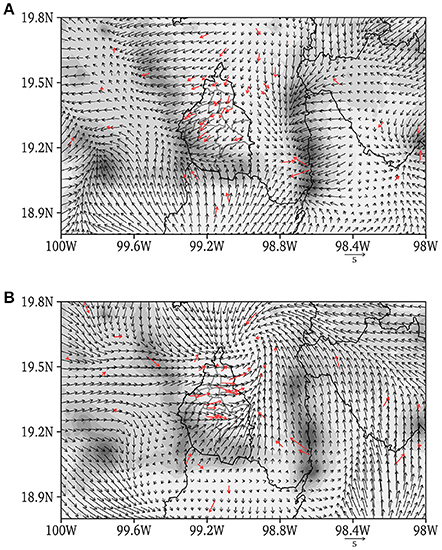
Figure 8. 10 m wind field (m/s) from the modified WRF version; vectors in red correspond to observations at surface stations: (A) 18:00 UTC 31 July 2014 morning valley mountain circulation; and (B) 02:00 UTC 1 August 2014 mountain–valley evening circulation.

WRF Summer Experiments

During the summer, the proper choice of the convection parameterization defines the forecasting ability to resolve the atmospheric characteristics of the MCMA. Unlike the winter conditions where the systems are more organized, summer precipitation is generated mostly by convective systems; these are characterized by small spatial scale and periods of life ranging from minutes to hours, and, consequently, the model predictability decreases owing to the characteristics of the weather systems and the incomplete description of the physical processes. To quantify the effect of the new WRF configuration, experiments were performed in forecast mode for the summer, specifically in July of 2014.

July 2014 Forecast of Temperature

The verification analysis for summer conditions (July 2014) was constructed with 24-h forecast experiments for gridded observations of daily surface temperature and precipitation. Changes in the local heating processes by surface sources led to adjustments in the atmosphere thickness and the temperature gradient, inducing variations in the circulation in the city (Figure 9). The effect of surface heating sources is reflected in the monthly-predicted tmp2m. The modified WRF version (Figure 10C) was better than the control version (Figure 10A) at simulating the monthly mean tmp2m. The simulated pattern is consistent with the observed field (Figure 10B), placing the maximum temperature on the urban sprawl and intensifying the horizontal gradient to the MCMA surroundings. However, in the northern part of the State of Mexico, the simulated temperature is colder than the observed. The extreme values show a spatial distribution similar to the expected patterns even though systematic errors in the forecast of maximum and minimum temperatures persist. The monthly mean maximum temperature (Figure 10F) confines the urban sprawl within a well-delimited area with a higher temperature than its surroundings. Nevertheless, control experiment doesn't have the skill to simulate the urban pattern (Figure 10D), whereas the observed pattern (Figure 10E) shows a weakening temperature gradient to the north of the MCMA. The spurious effect in the simulation is generated when there are two surfaces with very different properties, a situation that tends to intensify temperature and humidity gradients between the urban area and its surroundings. The field differences occur at a three-dimensional level and alter the vertical stability at a local scale and the formation and propagation of the storms. The simulated minimum temperature (Figure 10I) can describe the effect of the overnight warm air bubble remaining over the MCMA (Figure 10H), whereas in the control experiment (Figure 10G) it is confined to the city center only.

FIGURE 9

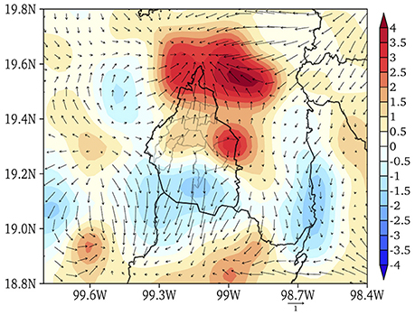
Figure 9. Sensitivity experiment with urban area of MCMA modified. 2 m air temperature (°C) difference for July 2014 between the control and the modified experiment at 17:00 UTC is shown in shading. The vectors show the 10 m wind differences (m/s).

FIGURE 10

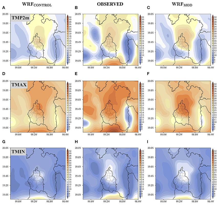
Figure 10. The 2 m temperature field (°C) simulated and observed for July 2014 (A) WRF control experiment (B) OBSERVED, and (C) WRF modified experiment. The maximum temperature field (°C) simulated and observed for July 2014 (D) WRF control experiment (E) OBSERVED, and (F) WRF modified experiment. The minimum temperature field (°C) simulated and observed for July 2014 (G) WRF control experiment (H) OBSERVED, and (I) WRF modified experiment.

Rainfall Forecasting of the 16 July 2014 Storm

Intense convective events occurred during 16 July 2014. The meteorological conditions were determined by an easterly tropical wave moving over the south and center of the country. By 00:00 UTC on 17 July 2014, a cyclonic circulation had become established over the MCMA.

The summer temperature, humidity, and atmospheric stability conditions activated the development of convective events at various points in the region. Two simulations (in forecast mode) were performed with the modified WRF version using the Kain-Fritsch (KF) (Kain, 2004) and the Betts-Miller-Janjic (BMJ) (Janjic, 1994, 2000) cumulus parameterization schemes and the WSM6 microphysics scheme (Hong and Lim, 2006) for both experiments. After a simulated 12 h, each experiment had captured the vertical temperature structure, but the KF scheme has a ~2°C negative bias near the surface (Figure 11A) and generates a saturated layer between 700 and 550 mb that is not shown in the observed profile. In the BMJ scheme, the negative bias in surface temperature is about 1°C and the moist vertical structure is similar to the observation. Although the observed profile shows saturation, the simulation profile shows a low dew point depression value at a certain level (Figure 11B). The simulated vertical distribution of moisture (Figure 11C) presents the changes, particularly near the surface (Pielke, 2002). In general, the BMJ scheme reproduces the horizontal and vertical field structures of temperature and humidity with high skill. However, it is not able to solve the shallow and deep convection adequately, and the center of convection activation are mislocated although the timing of precipitation is correctly reproduced (Figure 12).

FIGURE 11

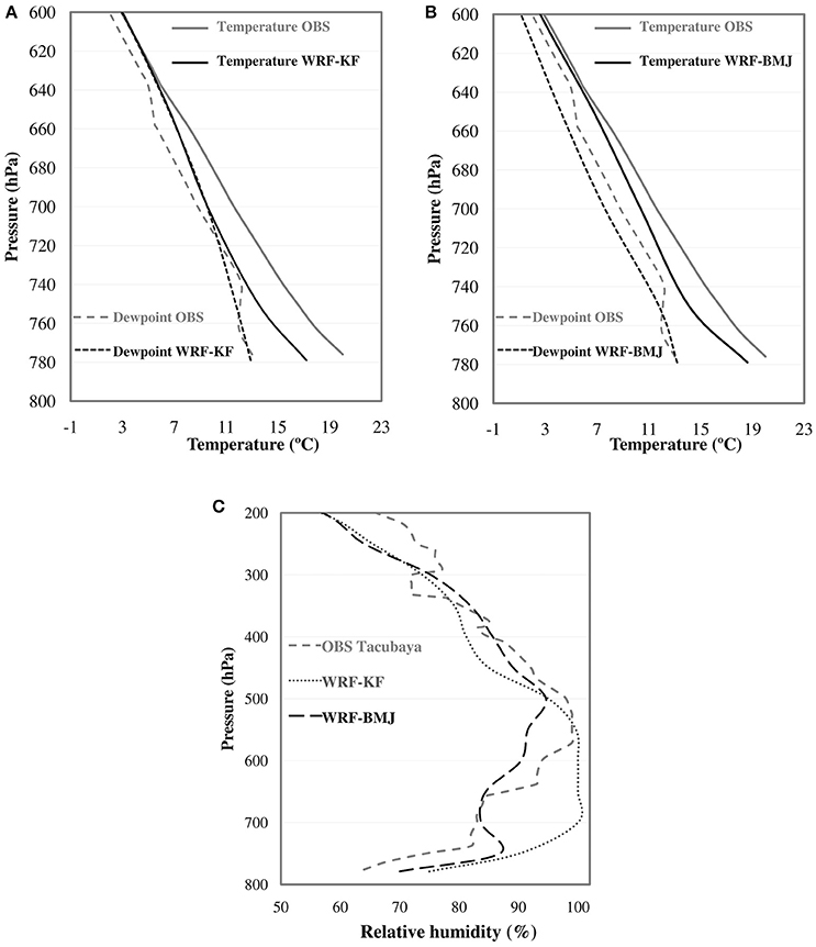
Figure 11. Vertical profiles at 00:00 UTC 17 July 2014; (A) Air temperature (°C) (solid line) and dew point temperature (°C) (dashed line). Tacubaya radiosonde (gray), WRF sounding using the KF convection scheme (black); (B) Tacubaya radiosonde, WRF sounding using the BMJ convection scheme (black); (C) Relative humidity profile (%). Tacubaya radiosondeo (gray dashed), WRF-BMJ scheme (black) and WRF-KF scheme (gray dots).

FIGURE 12

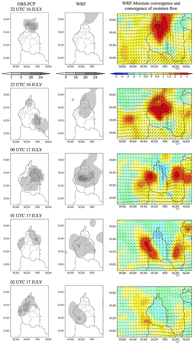
Figure 12. Hourly precipitation between 22:00 UTC 16 July and 02:00 UTC 17 July 2014: (left) observed; (center) forecast; (right) shaded area, moisture convergence (kg/kg/s) and surface to 650 mb convergence of moisture flow (kg/m/s).

The convective system began to develop around 22:00 UTC, generating precipitation at the north of MCMA. An analysis of humidity flux convergence from the surface to 650 mb level (near the storm steering level) shows a precipitation maximum at the northeast. By 23:00 UTC, the convergence center has moved south to the city center and moisture from the surrounding areas is transported to this region (Figure 12). At 00:00 UTC the convergence splits into two cores west of the city center and east of the State of Mexico (Figure 12). At this time the largest precipitation event occurs, and it is here that spatial differences between model and observation become evident. By 01:00 UTC the surface-650 mb moist convergence is established to the north of MCMA with the generation of convergence center over the mountain region and subsidence over the city center. The convection scheme BMJ fairly well reproduces the time evolution of the simulated precipitation for the period of 22:00 UTC 16 July to 02:00 UTC 17 July 2014. In general, the forecast tends to overestimate the precipitation (Figures 13A,B), with its 24 h accumulated precipitation reaching values near 60 mm in contrast to the observed accumulated precipitation of around 25 mm. Despite the difference in magnitudes, the most important result derived from these simulations is that the location and shape of the maximum precipitation predicted in the south-west of the MCMA are similar to the observed pattern (Magaña et al., 2003; Kozich, 2010; Aquino, 2012; Bravo-Carvajal et al., 2014; López-Bravo, 2015)

FIGURE 13

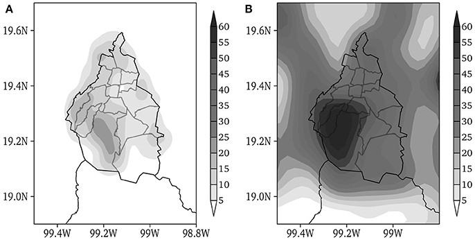
Figure 13. Accumulated precipitation between 12:00 UTC 16 July and 12:00 UTC 17 July 2014: (A) Observed (mm); (B) WRF predicted.

The changes in atmospheric stability are examined through a simulated temporal analysis of equivalent potential temperature (Θe) at Mexico City center (19.46°N, 99.10°W) for the two experiments. In both experiments, the convection schemes manage to simulate the unstable condition between 700 and 500 mb. However, the KF convective scheme shows the region of maximum instability at 22:00 UTC 16 July, 2 h earlier than the observed precipitation (Figure 14A). The conditions of relative humidity, vertical velocity, and convective available potential energy (CAPE) fall within the range required for the KF convection trigging (Kain, 2004) between 21:00 and 00:00 UTC. After the CAPE is completely consumed the scheme abruptly stops the convection development, and this leads to the stable saturated atmosphere at around 01:00 UTC, displacing the instability and moisture to 600–550 mb (blue line in Figure 14A). This post-convective state limits the development of new convective events, as was also found by Pielke (2002) and Stensrud et al. (2009).

FIGURE 14

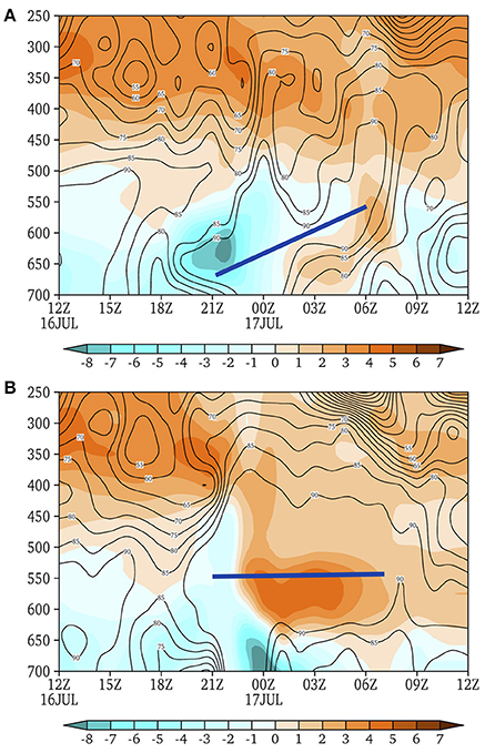
Figure 14. Atmospheric stability for Mexico City between 12:00 UTC 16 July and 12:00 UTC 17 July 2014: (A) KF parameterization; (B) BMJ parameterization. Shading: δΘe/δp (K/mb) Contours: relative humidity (%).

With the BMJ scheme, the maximum instability occurs at 00:00 UTC (Figure 14B). Although the development of convection has begun earlier, the scheme can achieve activation and position at the same place as the observation. In this scheme the instability is slowly removed, thereby modifying the moisture and temperature profiles, and keeping moist higher levels. Unlike the KF scheme, in the post-convective condition, the BMJ scheme maintains moisture for activation of subsequent convective events. However, the BMJ scheme has a little predictive skill in generating precipitation at the place and time observed (Kozich, 2010; López-Bravo, 2012).

The Orthogonal Empirical Functions (EOFs) technique (Wilks, 2011) was used to explain the difference between the precipitation values observed and the model, with the purpose of identifying the modes of variability in both cases. For July monthly precipitation data for the period 1979–2001 and the July 2014 WRF simulation, the first two modes of variability were extracted (only the first mode is presented). The first mode of variability (EOF1) of the observed precipitation explains 56% of the total variance (Figure 15A), and its pattern is associated with the occurrence of rainfall in the regions where the topographic elevation is considerable, showing the importance of orography in the distribution of precipitation over Mexico City. In this first mode, the west and south regions of the Mexico City present rain episodes more frequently compared to the central and eastern regions. The EOF1 pattern corresponds to the area where rains with greater frequency and intensity occur during summer months in Mexico City. The EOF 1 obtained from the modified WRF July 2014 simulation shows a total variance of 61% (Figure 15B). It captures the high dependence of the orographic component as shown by the first mode of precipitation obtained from the observations for the same period. This result indicates the positive impact of modifications introduced in the WRF model, which has improved the accuracy of the predicted meteorological variables and the derived fields (not observed in the unmodified WRF-not shown) to a spatial resolution of 12 km.

FIGURE 15

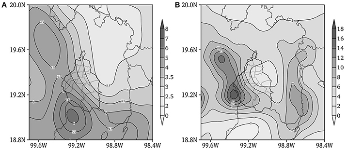
Figure 15. EOF analysis of the precipitation field for July 2014: (A) EOF constructed from surface observations; (B) EOF from the predicted precipitation field.

Discussion

The main aim of this work was to study the effect of land cover on the simulation and forecast of temperature and precipitation variables over MCMA Megacity during the summer season and in particular the month of July 2014. A new WRF model configuration is proposed. Firstly, an update of the MCMA urban land cover was carried out to improve the description of the surface processes in order to reproduce the convergence centers more adequately associated with storm development. Secondly, the hybrid nudging initialization method was examined to establish a spin up period to achieve a dynamic adjustment and thereby to obtain a coherent initial condition based on observations of surface stations and radiosonde integrated into cycles of 1 h and 00 and 12 UTC, respectively. Thirdly, sensitivity test studies were performed using KF and BMJ cumulus parametrization schemes. The BMJ scheme showed a better skill to describe the conditions of a tropical atmosphere in the summer season in the MCMA.

The results of this study show that the numerical weather prediction for MCMA is sensitive to resolution (12 km), weather systems, initialization (hybrid nudging), surface forcing, and model configuration. Although all these elements have been extensively explored in the literature, the characteristics of the MCMA are such that it was necessary to re-examine them to improve the quality of the forecasts generated by the WRF model for this particular region. A better initial condition and the implementation of a correction scheme (nudging) in the meteorological fields to get a dynamic adjustment have led to a simulation more closely resembling the conditions observed.

The forecasting and diagnostic accuracy of surface meteorological variables were improved through an adequate approximation of the land cover. The Noah land surface model reproduces the surface fluxes according to the spatial pattern and the temporal evolution of temperature, humidity, and winds observed and consequently reflect more reliably the changes in the dynamics and precipitation in the region. The WRF was able to capture the valley–mountain breeze, as well as the diurnal cycles of temperature and humidity. However, bias persists in the prognosis of extreme values (e.g., temperature). In the case of moisture variables, the model tends to remove moisture from low levels overnight, establishing a condition close to the surface that is drier than that observed.

The implementation of the adjustment period has also solved the generation of precipitation in the early hours of forecast and phasing the most intense events toward the afternoon hours, as it been characterized the diurnal cycle of precipitation observed for MCMA. Additionally, the problem of the inhomogeneous distribution of stations and errors due to the complex orography where changes in temperature and humidity are important in relatively small distances were avoided to some extent.

Conclusions

Summer weather predictability was examined using a new WRF model configuration and upgrade urban land cover (12 km). The results show that a more accurate short-range prediction for the MCMA can be attained, correcting the systematic spatial errors of the forecast and derivative variables. A better description of the temperature (an improvement ~ 30% over the urban area) requires that the effects of urbanization and Noah land surface scheme incorporated into the new WRF model configuration must be taken into account to improve the forecasting of extreme events. For the rainfall forecasting, the climatological pattern obtained shows a good adjustment to the orographic component, thereby reducing spatial uncertainty. However, a systematic bias of one order of magnitude persists in the precipitation magnitude.

The increase in temporal prediction skill was reflected with the implementation of the initial adjustment period (spin up time). Despite the forecasting improvements achieved, other systematic errors related to precipitation persist owing to the field of moisture distribution and the parameterization of moist convection. Concerning the correction of the initial condition, the current surface meteorological data and radiosondes are insufficient to describe the transport of moisture from the Gulf of Mexico adequately, a determining factor in the genesis of local storms in central Mexico. This could be improved with the assimilation of remote sensing products.

Author Contributions

CL-B: Mesoscale modeling, surface processes; EC: Tropical meteorology, ocean-atmosphere modeling; VM: Tropical meteorology, climate variability.

Conflict of Interest Statement

The authors declare that the research was conducted in the absence of any commercial or financial relationships that could be construed as a potential conflict of interest.

Acknowledgments

The National Council of Science and Technology (CONACYT) for the first author's MSc. scholarship 346260 and PAPIIT—UNAM IN106815.

References

Aquino, L. (2012). Impacto de la Urbanización Sobre la Dinámica de las Tormentas en el Valle de México. M.Sc dissertation, Posgrado en Ciencias de la Tierra UNAM, 85.

Bravo-Carvajal, I., Garnica-Peña R., López-Bravo C., and Alcántara-Ayala I. (2014). “Landslide susceptibility mapping using remote sensing and GIS: Nueva Colombia, Chiapas, Mexico,” in Landslide Science for a Safer Geoenvironment, eds K. Sassa, P. Canuti, and Y. Yin (Springer International), 405–411.

Google Scholar

Chen, F., and Dudhia, J. (2001). Coupling an advanced land surface–hydrology model with the Penn State–NCAR MM5 modeling system. Part I: model implementation and sensitivity. Mon. Weather Rev. 129, 569–585. doi: 10.1175/1520-0493(2001)129<0569:CAALSH>2.0.CO;2

CrossRef Full Text | Google Scholar

Chen, F., Mitchell, K., Schaake, J., Xue, Y., Pan, H-L., Koren, V., et al. (1996). Modeling of land surface evaporation by four schemes and comparison with FIFE observations. J. Geophys. Res. Atmos. 101, 7251–7268. doi: 10.1029/95JD02165

CrossRef Full Text | Google Scholar

Cheng, W. Y., and Steenburgh, W. J. (2005). Evaluation of surface sensible weather forecasts by the WRF and the Eta Models over the Western United States. Weather Forecast. 20, 812–821. doi: 10.1175/WAF885.1

CrossRef Full Text | Google Scholar

Cressman, G. P. (1959). An operational objective analysis system. Mon. Weather Rev. 87, 367–374. doi: 10.1175/1520-0493(1959)087<0367:AOOAS>2.0.CO;2

CrossRef Full Text | Google Scholar

Ek, M. B., Mitchell, Y., Lin, K. E., Rogers, E., Grunmann, P., Koren, V., et al. (2003). Implementation of Noah land surface model advances in the National Centers for Environmental Prediction operational mesoscale Eta model. J. Geophys. Res. Atmos. 108:8851. doi: 10.1029/2002JD003296

CrossRef Full Text | Google Scholar

Fast, J. (1995). Mesoscale modeling and four-dimensional data assimilation in areas of highly complex terrain. J. Appl. Meteorol. 34, 2762–2782. doi: 10.1175/1520-0450(1995)034<2762:MMAFDD>2.0.CO;2

CrossRef Full Text | Google Scholar

Hong, S.-Y., and Lim, O. J. (2006). The WRF single-moment 6-class microphysics scheme (WSM6). J. Korean Meteorol. Soc. 42, 129–151. doi: 10.1155/2010/707253

CrossRef Full Text | Google Scholar

Hong, S.-Y., Noh, Y., and Dudhia, J. (2006). A new vertical diffusion package with an explicit treatment of entrainment processes. Mon. Weather Rev. 134, 2318–2341. doi: 10.1175/MWR3199.1

CrossRef Full Text | Google Scholar

INEGI (2010). Conteo de Población y Vivienda 2010. Indicadores del censo general de Población y vivienda, INEGI, México.

Janjic, Z. I. (1994). The step-mountain eta coordinate model: further developments of the convection, viscous sublayer, and turbulence closure schemes. Mon. Weather Rev. 122, 927–945. doi: 10.1175/1520-0493(1994)122<0927:TSMECM>2.0.CO;2

CrossRef Full Text | Google Scholar

Janjic, Z. I. (2000). Comments on “Development and evaluation of a convection scheme for use in climate models”. J. Atmos. Sci. 57, 3686–3686. doi: 10.1175/1520-0469(2000)057<3686:CODAEO>2.0.CO;2

CrossRef Full Text | Google Scholar

Jáuregui, E. (2000). El Clima de la Ciudad de México, Vol. 1. Mexico: Plaza y Valdés. 131.

Jáuregui, E., and Romales, E. (1996). Urban effects on convective precipitation in Mexico City. Atmos. Environ. 30, 3383–3389. doi: 10.1016/1352-2310(96)00041-6

CrossRef Full Text | Google Scholar

Jiménez, P. A., and Dudhia, J. (2013). On the ability of the WRF model to reproduce the surface wind direction over complex terrain. J. Appl. Meteorol. Climatol. 52, 1610–1617. doi: 10.1175/JAMC-D-12-0266.1

CrossRef Full Text | Google Scholar

Joyce, R. J., Janowiak, J. E., Arkin, P. A., and Xie, P. (2004). CMORPH: a method that produces global precipitation estimates from passive microwave and infrared data at high spatial and temporal resolution. J. Hydrometeorol. 5, 487–503. doi: 10.1175/1525-7541(2004)005<0487:CAMTPG>2.0.CO;2

CrossRef Full Text | Google Scholar

Kain, J. S. (2004). The Kain-Fritsch convective parameterization: an update. J. Appl. Meteorol. 43, 170–181. doi: 10.1175/1520-0450(2004)043<0170:TKCPAU>2.0.CO;2

CrossRef Full Text | Google Scholar

Klein Tank, A. M. G., Wijngaard, J. B., Können, G. P., Böhm, R., Demarée, G., Heino, R., et al. (2002). Daily dataset of 20th-century surface air temperature and precipitation series for the European climate assessment. Int. J. Climatol. 22, 1441–1453. doi: 10.1002/joc.773

CrossRef Full Text | Google Scholar

Kozich, P. J. (2010). Overview of Mexico City Meteorological Conditions Using Observations and Numerical Simulations. Ph.D. dissertation, Saint Louis University, 191.

Lee, T., Pielke, R., Kessler, R., and Weaver, J. (1989). Influence of cold pools downstream of mountain barriers on downslope winds and flushing. Mon. Weather Rev. 117, 2041–2058. doi: 10.1175/1520-0493(1989)117<2041:IOCPDO>2.0.CO;2

CrossRef Full Text | Google Scholar

Liu, Y., Bourgeois, A., Warner, T., Swerdlin, S., and Hacker, J. (2005). “Implementation of observation-nudging based FDDA into WRF for supporting ATEC test operations,” in 2005 WRF Users Workshop (Boulder, CO).

Google Scholar

López-Bravo, L. (2012). Evaluación de la Calidad del Pronóstico Numérico del Tiempo en la Ciudad México. BE dissertation, Facultad de Ingeniería UNAM. 68.

López-Bravo, L. (2015). Evaluación de la Predictibilidad del Tiempo Atmosférico en el Valle de México. M.Sc dissertation, Posgrado en Ciencias de la Tierra UNAM. 109.

Magaña, V., Pérez, J., and Méndez, M. (2003). Diagnosis and prognosis of extreme precipitation events in the Mexico City basin. Geofís. Int. 42, 247–260. doi: 10.22201/igf.00167169p.2003.2.269

CrossRef Full Text

Mesinger, F., DiMego, G., Kalnay, E., Mitchell, K., Shafran, P. C., Ebisuzaki, W., et al. (2006). North American regional reanalysis. Bull. Am. Meteorol. Soc. 87, 343–360. doi: 10.1175/BAMS-87-3-343

CrossRef Full Text | Google Scholar

Minder, J. R., Mote, P. W., and Lundquist, J. D. (2010). Surface temperature lapse rates over complex terrain: lessons from the Cascade mountains. J. Geophys. Res. Atmos. 115, 1–13. doi: 10.1029/2009JD013493

CrossRef Full Text | Google Scholar

Mölders, N. (2011). Land-use and Land-Cover Changes: Impact on Climate and Air Quality. Vol. 44. Springer Science & Business Media, 187. doi: 10.1007/978-94-007-1527-1_3

CrossRef Full Text

National Centers for Environmental Prediction, National Weather Service, NOAA, U.S. Department of Commerce (2015). NCEP GFS 0.25 Degree Global Forecast Grids Historical Archive. Research Data Archive at the National Center for Atmospheric Research, Computational and Information Systems Laboratory, Boulder, CO.

Oke, T. R. (1987). Boundary Layer Climates 2nd Edn., London: Routledge, 423.

Pielke, R. A. Sr. (2002). Mesoscale Meteorological Modeling, 2nd Edn. San Diego, CA: Academic Press, 676.

Ray, P. (1986). Compilation. Mesoscale Meteorology and Forecasting. Boston, MA: American Meteorological Society. 785.

Seaman, N. L., Stauffer, D. R., and Lario-Gibbs, A. M. (1995). A multiscale four-dimensional data assimilation system applied in the San Joaquin Valley during SARMAP. Part I: modeling design and basic performance characteristics. J. Appl. Meteorol. 34, 1739–1761. doi: 10.1175/1520-0450(1995)034<1739:AMFDDA>2.0.CO;2

CrossRef Full Text | Google Scholar

Shafran, P. C., Seaman, N. L., and Gayno, G. A. (2000). Evaluation of numerical predictions of boundary layer structure during the Lake Michigan Ozone study. J. Appl. Meteorol. 39, 412–426. doi: 10.1175/1520-0450(2000)039<0412:EONPOB>2.0.CO;2

CrossRef Full Text | Google Scholar

Sharma, A., Fernando, H. J. S., Hamlet, A. F., Hellmann, J. J., Barlage, M., and Chen, F. (2017). Urban meteorological modeling using WRF: a sensitivity study. Int. J. Climatol. 37, 1885–1900. doi: 10.1002/joc.4819

CrossRef Full Text | Google Scholar

Slingo, J., and Palmer, T. (2011). Uncertainty in weather and climate prediction. Phil. Trans. R. Soc. A, 369, 4751–4767. doi: 10.1098/rsta.2011.0161

PubMed Abstract | CrossRef Full Text | Google Scholar

Smith, W. H., and Sandwell, D. T. (1997). Global sea floor topography from satellite altimetry and ship depth soundings. Science, 277, 1956–1962. doi: 10.1126/science.277.5334.1956

CrossRef Full Text | Google Scholar

Stauffer, D. R., and Seaman, N. L. (1994). Multiscale four-dimensional data assimilation. J. Appl. Meteorol. 33, 416–434. doi: 10.1175/1520-0450(1994)033<0416:MFDDA>2.0.CO;2

CrossRef Full Text | Google Scholar

Stauffer, D. R., Seaman, N. L., and Binkowski, F. S. (1991). Use of four-dimensional data assimilation in a limited-area mesoscale model Part II: effects of data assimilation within the planetary boundary layer. Mon. Weather Rev. 119, 734–754. doi: 10.1175/1520-0493(1991)119<0734:UOFDDA>2.0.CO;2

CrossRef Full Text | Google Scholar

Stensrud, D. J. et al. (2009). Convective-scale warn-on-forecast: A vision for 2020. Bull. Am. Meteorol. Soc. 90, 1487–1499. doi: 10.1175/2009BAMS2795.1

CrossRef Full Text | Google Scholar

Taylor, K. E. (2001). Summarizing multiple aspects of model performance in a single diagram. J. Geophys. Res. 106, 7183–7192. doi: 10.1029/2000JD900719

CrossRef Full Text | Google Scholar

Wang, D., Miao, J., and Zhang, D. L. (2015). Numerical simulations of local circulation and its response to land cover changes over the Yellow Mountains of China. J. Meteorol. Res. 29, 667–681. doi: 10.1007/s13351-015-4070-6

CrossRef Full Text | Google Scholar

Wang, W., Bruyère C Duda, M., Dudhia, J., Gill, D., Kavulich, M., et al. (2014). ARW Version 3 Modeling System User's Guide. Mesoscale & Microscale Meteorology Division; National Center for Atmospheric Research. Avaliable online at: http://www2.mmm.ucar.edu/wrf/users/docs/user_guide_V3/ARWUsersGuideV3.pdf

Warner, T. T. (2010). Numerical Weather and Climate Prediction. Cambridge: Cambridge University Press, 526. doi: 10.1017/CBO9780511763243

CrossRef Full Text | Google Scholar

Wilks, D. S. (2011). Statistical Methods in the Atmospheric Sciences. 3nd Edn. San Diego, CA: Academic Press. 704.

Wolyn, P. G., and McKee, T. B. (1989). Deep stable layers in the intermountain western United States. Mon. Weather Rev. 117, 461–472. doi: 10.1175/1520-0493(1989)117<0461:DSLITI>2.0.CO;2

CrossRef Full Text | Google Scholar

Yu, W., Liu, Y., and Warner, T. (2007). “An evaluation of 3DVAR, nudging based FDDA and a hybrid scheme for summer convection forecast using WRF-ARW model,” in 18th Conference on Numerical Weather Prediction (Boulder, CO), 25–29.