Representation of Ocean-Atmosphere Processes Associated with Extended Monsoon Episodes over South Asia in CFSv2

In the present study, we analyze 30-years output from free run solutions of Climate forecast system version 2 (CFSv2) coupled model to assess the model's representation of extended (>7 days) active and break monsoon episodes over south Asia. Process based diagnostics is applied to the individual and composite events to identify precursor signals in both ocean and atmospheric variables. Our examination suggests that CFSv2, like most coupled models, depicts systematic biases in variables important for ocean-atmosphere interactions. Nevertheless, model solutions capture many aspects of monsoon extended break and active episodes realistically, encouraging us to apply process-based diagnostics. Diagnostics reveal that sea surface temperature (SST) variations over the northern Bay of Bengal where the climatological mixed-layer is thin, lead the in-situ precipitation anomalies by about 8 (10) days during extended active (break) episodes, and the precipitation anomalies over central India by 10–14 days. Mixed-layer heat budget analysis indicates for a close correspondence between SST tendency and net surface heat flux (Q_net). MSE budgets indicate that horizontal moisture advection to be a coherent precursor signal (~10 days) during both extended break (dry advection) and active (moist advection) events. The lead timings in these precursor signals in CFSv2 solutions will be of potential use to monitor and predict extended monsoon episodes. Diagnostics, however, also indicate that for about 1/3 of the identified extended break and active episodes, inconsistencies in budget terms suggest precursor signals could lead to false alarms. Apart from false alarms, compared to observations, CFSv2 systematically simulates a greater number of extended monsoon active episodes.

Introduction

Rainfall during the Indian summer monsoon (ISM) season (June–September) fluctuates between active and break spells. In any given year, the occurrence of such spells for extended periods (≥ 7 days) impacts the seasonal-mean rainfall, with measurable socio-economic impacts. It is recognized that the monsoon and the tropical Indian Ocean are intrinsically a coupled system (e.g., Annamalai et al., 2017). In coupled models employed for operational prediction of the monsoons it is therefore imperative to examine if the leading precursor signals in ocean and atmospheric variables that influence these extended monsoon episodes are realistically represented. With that goal in mind, here we diagnose the representation of extended active and break monsoon episodes in the Climate Forecast System version 2 (CFSv2) integrations, and then assess whether the leading thermodynamical processes are faithfully represented in the solutions. Such a process-based diagnostic is necessary to appreciate the strengths and limitations in any model parameterization schemes. It should be mentioned here that under the auspices of the National Monsoon Mission initiated by the Government of India, CFSv2 is being employed for monsoon prediction over the Indian region.

Background

In climate models, a realistic simulation of the mean monsoon state is pre-requisite for assessing the representation of variability at any scales (e.g., Sperber and Palmer, 1994; Turner et al., 2005; Annamalai et al., 2007). Despite dedicated efforts by the modeling community, systematic errors in the simulation of monsoon precipitation and tropical Indian Ocean SST still exist, precluding any detailed assessment of monsoon variability. Specifically, compared to observed climatology, almost all models simulate a dry (wet) bias over continental India extending into the northern Bay of Bengal (western Arabian Sea), and cold SST bias over most parts of the tropical Indian Ocean (Levine et al., 2013; Sperber et al., 2013). Model errors exist throughout the annual cycle and not just pertinent for the summer (Annamalai et al., 2017).

Diagnosing CFSv2 integrations several studies have identified similar dry bias in seasonal mean precipitation climatology over continental India and cold SST bias over the tropical Indian Ocean (Goswami et al., 2014; Saha S. K. et al., 2014; Abhik et al., 2016; Shukla and Huang, 2016). Quantitatively, the model simulates a dry bias of −4 to −6 mm/day over the central and northern parts of India and a wet bias (>3 mm/day) along the windward side of the mountain regions along the Burmese coast. Regarding SST climatology, a cold bias (−0.2 to −1.0°C) in the western Indian Ocean and a warm bias (0.5–1.0°C) in the western Pacific (Shukla and Zhu, 2014) are noted. In summary, the climatological biases in CFSv2 are similar to those of many present-day coupled climate models. We recognize that such systematic errors in a time-mean sense arise due to errors in both ocean and atmospheric components of the coupled model (Annamalai et al., 2017), and could impact the simulated variance across all time scales.

Examining year wise statistics of observed extended monsoon episodes, Prasanna and Annamalai (2012) hypothesized that they arise due to interactions between tropical intraseasonal variability and boundary forcing such as SST anomalies during El Niño. While numerous studies have examined CFSv2 fidelity in representing El Niño (Kim et al., 2012; Chaudhari et al., 2013; Saha S. K. et al., 2014 and references there in), only few have diagnosed aspects of monsoon intraseasonal variability. During summer, the dominant observed intraseasonal variations in precipitation are associated with the northward-propagating convective events that originate over the equatorial Indian Ocean and imprint on the active and break phases of rainfall over continental India (Yasunari, 1979; Sikka and Gadgil, 1980). In the model, such poleward-migrating convective anomaly events do occur in the filtered (~20–100 days) precipitation data, but compared to observations, biases in amplitude, structure, and propagation speed are noted (Goswami et al., 2014; Saha S. K. et al., 2014; Shukla and Zhu, 2014). While the observed tilted rain band extending from northwest Indian to near-equatorial Pacific is reasonably represented in the model, the simulated intraseasonal variance (20–100 days) in precipitation is unrealistically large. Here, while diagnosing and interpreting the space-time evolution of model simulated intraseasonal variability these model limitations are borne in mind.

While the existence of northward propagating intraseasonal variability may be of atmospheric origin, their statistical properties such as amplitude, time scales etc are influenced by intraseasonal SST anomalies (Fu et al., 2003) implying the role of coupled ocean-atmosphere interactions during their life cycle. To understand the processes that shape intraseasonal SST variations, several studies emphasized the importance of air-sea fluxes, both in observations (Bhat et al., 2001; Sengupta and Ravichandran, 2001) and models (Fu et al., 2003). Furthermore, maximum amplitude of subseasonal SST variability occurs in regions where the mixed layer (ML) is thin (Duvel and Vialard, 2007; Vialard, 2012), a feature most climate models fail to capture over the tropical Indian Ocean (Nagura et al., 2017).

In summary, while past studies have examined model's ability in simulating poleward intraseasonal precipitation variability and also possible SST-precipitation association at this time scale (e.g., Sharmila et al., 2013; Saha S. K. et al., 2014), to the best of our knowledge no process-based diagnostics are applied to identify model's fidelity in representing processes, both atmospheric and oceanic, that determine the life cycle of extended monsoon episodes.

Present Study

Here, with a goal to assess model's representation of extended monsoon episodes and associated processes we diagnose a 30-years integration of CFSv2. It is expected such a detailed examination will identify physically based precursors to monitor the extended episodes, as well highlight model's strengths and limitations, and importantly identify false alarms, if any. To motivate our focus, Figures 1A,B show histograms of active and break events over central India from CFSv2 and 13 years of Tropical Rainfall Measuring Mission (TRMM) observations (definitions of active and break events are mentioned in section Model, Observations, and Methodology). Consistent with earlier reanalysis studies (Prasanna and Annamalai, 2012; Mohan and Annamalai, under review), CFSv2 frequency distributions for break events agree well with observations in that short (3 days) and extended (7 days or more) events occur more frequently. Analysis with IMD observations (Figure not shown) also exhibits similar frequency distribution of extended episodes, but with increase in number of events. In contrast, the model's ability to capture the distribution of active events is severely limited. Specifically, CFSv2 captures more frequent (less frequent) occurrences of extended (short) active conditions. It is well-known, that CFSv2 model basic state in precipitation is very dry (for ex., Goswami et al., 2014; Saha S. K. et al., 2014) and its standard deviation also smaller compared to observations, perhaps resulted in more number of extended active days. Thus, the frequency of extended events is outnumbered than the observations. Despite this limitation, in the context of the present study, we are interested in understanding how closely the processes identified in the model agree with those identified in reanalysis products (and not the number of events).

FIGURE 1

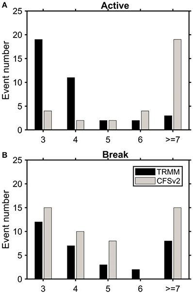
Figure 1. Histogram of (A) active (B) break days computed from TRMM rainfall observations (black bars) and CFSv2 simulations (gray bars) averaged over central India (15–25°N, 72–85°E). x-axis represents the number of days.

Prior to examining extended episodes, we assess the simulated climatological distributions in regional precipitation and SST and compare them with observations and highlight model systematic biases. Then, employing composite analysis as in Prasanna and Annamalai (2012) and Mohan and Annamalai, (under review), we study the space-time evolution of key variables that describe the life cycle of monsoon extended episodes. Here, we will isolate how typical extended episodes differ from traditional active-break cycles of monsoon. Then, for the constructed composites, we apply vertically integrated moist static energy (MSE) budget to identify atmospheric precursors. Finally, mixed-layer heat budget is applied to identify the oceanic precursor, particularly SST fluctuations over the Bay of Bengal. To understand how the atmospheric and oceanic processes in an individual extended episode are consistent with the composite evolution, we also examine individual events. By doing so, we identify incoherency among the model processes implying false alarms in the simulation that needs attention, because CFSv2 is employed for extended range prediction of monsoon rainfall over India.

Major results are the following. The SST anomalies over the northern Bay of Bengal lead in-situ precipitation anomalies by ~8–10 days, and they lead the precipitation anomalies over central India by ~12 days. On a similar note, vertically integrated, MSE budget analysis shows that dry (moist) air advection leads extended break (active) episodes over central India by ~8 days. Our results provide precursors, both in oceanic and atmospheric variables that could be exploited for monitoring and prediction of extended monsoon episodes over continental India.

The remaining part of the manuscript is organized as follows. section Model, Observations, and Methodology describes the CFSv2 model simulation and observations, and reanalysis products used for validation, and briefly discuss the MSE and ML budget methods. In section Basic State and Intraseasonal Variability, model's ability in representing seasonal mean climatologies of key variables and its fidelity in simulating the space-time evolution of precipitation during extended monsoon episodes are presented. In section Budget Diagnostics, we examine ML heat and MSE budgets. Summary of our findings and their implication are provided in section Summary and Discussion.

Model, Observations, and Methodology

In this section, we first provide an overview of our coupled model and the observational data we use to validate it. Then, we describe the MSE and ML heat budgets we use to identify model processes. Finally, we provide a precise definition of the extended active and break episodes that occur in our solution.

Coupled Model

For the present study, we use the latest version of NCEP's climate-forecast-system coupled model (CFSv2), run freely without data assimilation (Saha S. K. et al., 2014). Its atmospheric component is the NCEP Global Forecast System (GFS), with a horizontal resolution of T126 (~100 km) and 64 sigma-pressure hybrid layers from the surface to 0.26 hPa. The model includes a 3-layer interactive global sea-ice model, as well as a 4-level land-surface model with interactive vegetation (Ek et al., 2003). The oceanic component is the Geophysical Fluid Dynamics Laboratory (GFDL) Modular Ocean Model version 4 (MOM4; Griffies et al., 2004), with meridional and zonal resolutions of 0.25° and 0.5°, respectively, from 10°S to 10°N and uniform a horizontal resolution of 0.5° north of 30°N and 40 levels in the vertical. Initial conditions for the atmosphere and the ocean models are taken from NCEP Climate Forecast System Reanalysis (CFSR).

Model runs were carried out at the Center for Ocean-Land-Atmosphere studies (COLA). We analyze 30 years of daily output of three-dimensional (3-days) atmospheric and oceanic variables, as well as surface and top radiative fluxes for the atmosphere and mixed-layer thickness (MLT) for the ocean. All model data is interpolated onto a 0.5° × 0.5° grid.

Observations and Reanalysis Data

For validating the budget diagnostics from the CFSv2 model simulations, we use the CFSR reanalysis products (Saha et al., 2010), which cover the period 1981–2010 for both the atmosphere and ocean. Note that although, CFSR and CFSv2 came from same frame work, certain differences exist in terms of physical parameterizations and tuning parameters. For instance, (a) In new CFSv2 virtual temperature used as prognostic variable instead of enthalpy in CFSR, (b) Cloud-radiation interaction scheme in CFSR is (Rapid radiative transfer Model) RRTM, whereas in CFSv2, it is advanced cloud-radiation scheme applied to RRTM to address the unresolved variability of layered clouds. More details of the model can be found in Saha et al. (2010) and Saha S. K. et al., (2014). For validating precipitation and SST, we use the TRMM precipitation product 3B42 (also known as the TRMM Multi satellite Precipitation Analysis, TMPA) with spatial and temporal resolutions of 0.25° and 3 h, and TRMM Microwave imager (TMI) derived daily SST with a spatial resolution of 0.25° (Huffman et al., 2007). The satellite observations cover the period 1998–2014. Finally, Argo-derived monthly MLT monthly climatology is used for model validation. Available Argo profiles are screened for quality control (Holte and Talley, 2009) and interpolated onto a 1° × 1° grid, and various statistical techniques are applied to generate monthly MLT data for the period 2000–2015. More details of the MLT data can be found from http://mixedlayer.ucsd.edu.

Budget Diagnostics

Mixed-Layer Temperature Budget

To understand and quantify the upper-ocean processes that may govern ML temperature (or SST) variations, we use the temperature-tendency equation for the ML given by

$\begin{array}{ll}\frac{\partial T_{ml}}{\partial t}=\frac{Q_{net}-Q}{{\rho }_0{C}_{p}h}-V·\nabla T_{ml}-\frac{w_e\left(T_{ml}-T_d\right)}{h}+R.& (1)\end{array}$

In (1), T_ml is the mixed-layer temperature, T_d is the temperature at the bottom of the mixed layer, ρ₀ is a background value of sea-water density (1,026 kgm⁻³), C_p is the specific heat capacity of seawater (3,986 J kg⁻¹K⁻¹); h is the mixed layer thickness, Q_net is the net surface heat flux (Wm⁻²), Q is the shortwave radiation penetrating the mixed layer depth, w_e is the entrainment rate (ms⁻¹), and R is the residual term in the budget equation. The horizontal-advection term is $V·\nabla T_{ml}=u\frac{\partial T_{ml}}{\partial x}+v\frac{\partial T_{ml}}{\partial y},$ where u and v are zonal and meridional currents averaged within the mixed layer. More details can be found in Sengupta et al. (2001).

MSE Budget

Combining the temperature and moisture equations, convective heating and the moisture sink cancel when vertically integrated, and the balance is then among the net flux into the column and stability (Annamalai, 2010). Therefore, MSE budget becomes the leading thermodynamic constraint in deep convective regions (Neelin and Held, 1987; Neelin and Su, 2005). Several studies have utilized MSE budget as a diagnostic tool to study the tropical intraseasonal variability (e.g., Maloney, 2009; Annamalai, 2010; Prasanna and Annamalai, 2012). The approximate vertically integrated MSE budget can be given by

$\begin{array}{ll}\langle \frac{\partial m}{\partial t}\rangle =-\langle V·\nabla q\rangle -\langle V·\nabla T\rangle -\langle \omega \frac{\partial m}{\partial p}\rangle +LH+SH+F_{rad}+R& (2)\end{array}$

where m = s + q is known as MSE and s is dry static energy, q is specific humidity, T is temperature, SH and LH are sensible and latent heat fluxes, and F_rad is net radiative heating for the air column (i.e., the difference between the net fluxes across the bottom and top of the atmosphere). “R” in equation (2) indicates the residuals in budget terms. Angle brackets represent a mass-weighted, vertical integration over the column from 1,000 to 100 hPa. For both MSE and ML temperature budgets, we apply a 5-point running-mean filter to remove small-scale fluctuations, and no other temporal filtering is applied.

In order to identify the contributions of moisture and wind, we decompose the moisture-advection term into mean (superscript “o”) and perturbation (primed and double-primed) components as

$\begin{array}{ll}V·\nabla q=V^o·\nabla q^{\prime }+V^{\prime }·\nabla q^o+V·\nabla q+V^{″}·\nabla q^{″},& (3)\end{array}$

Where the primes indicate the anomalous moisture and the quantities containing primes are as follows; V^o·∇q′ is the advection associated with the climatological wind acting on the anomalous moisture gradients, V′·∇q^o is advection due to anomalous wind acting on climatological moisture gradients, and the last two terms are the anomalous wind acting on anomalous moisture gradients and turbulent fluctuations in the moisture fields or eddy variability respectively. An examination equation 3 shows that the contributions of V′·∇q^o during breaks, and V^o·∇q′ during active events dominate (section Budget Diagnostics).

Definition of Extended Episodes

An extended active (break) is considered to have happened if the area-averaged rainfall anomaly over central India (15–25°N, 72–85°E; termed region NCEN) is greater (less) than one standard deviation (σ) and persists for 7 continuous days or more. NCEN covers the region where there is a local maximum in modeled, daily rainfall variance (Figure 4). It is slightly different from averaging regions used in other studies (Prasanna and Annamalai, 2012; Mohan and Annamalai, under review), because in CFSv2 the simulated maximum variance over continental India is shifted southward compared to observations. The procedure yielded 17 (26) extended break (active) events. Similar procedure is then applied to CFSR precipitation data resulting in 25 (27) extended break (active) events.

Strong Monsoon Episodes

As mentioned in section Present Study, we will employ ML and MSE budget analysis on, (1) individual strong episodes and (2) composite of the events. Here, rainfall anomalies of the events, obtained by the procedure outlined in section Definition of Extended Episodes are analyzed from 30 days prior to 30 days later, with day 0 being the rainfall maximum over central India. We then constructed time series of the key variables of SST and precipitation for the identification of strong episode.

For all model identified extended break and active events, we examined the temporal evolution of precipitation (SST) anomalies averaged over central India (northern BoB), and identified those events that depicted “very high” values (~1.5 σ) at day 0 (−10 days) for precipitation (SST), and termed “strong episodes.” By applying these criteria, relatively strong episodes are obtained and then one such episode is analyzed for budget diagnostics, which will be discussed elaborately in section Budget Diagnostics.

Basic State and Intraseasonal Variability

In this section, we describe characteristics of the seasonal-mean (section Basic State) and sub-seasonal variability (section Subseasonal Properties) present in our solution.

Basic State

Figure 2 shows the seasonal-mean biases in precipitation (Figure 2A), SST (Figure 2B) and MLT (Figure 2C) over the south Asian region. We attempt to interpret the inter-linked biases among these variables that possibly suggest the intricate difficulties in simulating the monsoon basic state.

FIGURE 2

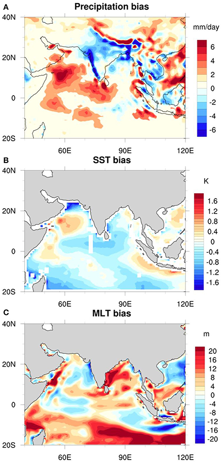
Figure 2. Seasonal-mean (June–September) climatological biases of: (A) rainfall in mm/day; (B) SST (°K) relative to observations; and (C) MLT referenced to CFSR values. Rainfall from TRMM observation (1998–2010); mean SST climatology from TMI observations.

Compared to observations, model simulates excess rainfall (4–5 mm/day) over the western Indian Ocean with a local maximum over the Arabian Sea. Wet bias is also noted over the near-equatorial Indian Ocean, and parts of the South China Sea. Model dry biases are prominent over most parts of the Indian subcontinent and in the far-northern BoB with a local maximum over northwest India, and along the Western Ghats and southern slopes of the Himalayas. The spatial distribution in precipitation bias in CFSv2 is akin to biases in present-day coupled models (e.g., Sperber et al., 2013). The model SST bias exhibits warmer SST (~2° K) over the central-western Arabian Sea, and the marginal seas of the Maritime Continent, which roughly coincides with regions of wet bias, as well as thin MLT biases, to a certain extent. Additionally, a one-to-one bias between cold SST and thicker MLT are noticeable in most parts of the tropical Indian Ocean, features that are not associated with negative precipitation bias. While the magnitude of precipitation or SST biases could differ based on the choice of observational products or higher-resolution (T382) CFSv2 simulations, the spatial patterns in biases are robust features (Saha S. K. et al., 2014; Abhik et al., 2016). In climate models, Annamalai et al. (2017) argued that errors in the representation of equatorial Indian Ocean processes cause dry (wet) bias over western Arabian Sea (continental India), a topic of ongoing research with CFSv2 solutions.

Apart from spatial patterns in basic-state, we also examined the model's ability in representing the annual cycle of the SST and precipitation over three oceanic regions and also over Indian land regions (Figure 3), regions that show substantial variance at subseasonal timescales (Figure 4). As regards SST, over both the BoB and Arabian Sea (AS), the observed semi-annual cycle is represented well by the model. In particular, during the monsoon season SST over the BoB remains above 28°C, and the model simulates peak rainfall during the months of July and August. In other seasons, however, model simulates a cold SST bias (~1°C) during the pre-monsoon season (March – May) and a warm bias (~0.5°C) during winter. In contrast to the BoB, the observed “rainy season” over the AS is much shorter (<2 months; Figure 3D), perhaps due to rapid cooling of SST caused by oceanic processes. In general, over AS winds blow from southwest in May and the ocean responds quickly along the coastal boundaries. The southwesterly winds gradually strengthen and as a result peak in observed rainfall annual cycle during June is seen, when monsoon starts over continental India. Further, southwest monsoon reaches its peak in July and in response low-level south westerly flow (or Somali current) over AS is also gets intensified. However, strong ocean upwelling due to Ekman convergence increases mixed layer thickness and rapid SST cooling resulting in subdued convection (McCreary et al., 1993). Here, during the pre-monsoon season, the rise in SST is slow and weak, and the maximum is phase shifted by a month with an imprint in the simulated rainfall annual cycle (Figure 3D). While the reasons for the simulated errors in SST are unclear, a possible candidate is the erroneous MLT over the AS throughout the annual cycle (not shown), a feature present in the CFSR products with which the model is initialized.

FIGURE 3

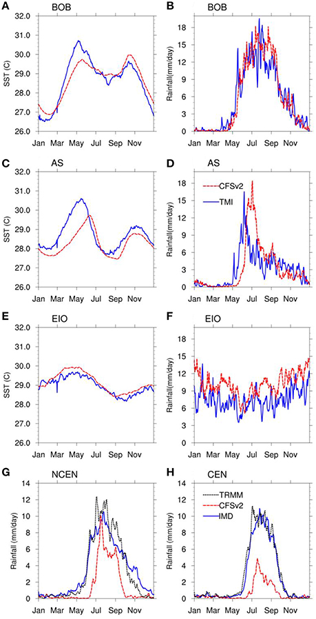
Figure 3. Annual cycle of SST (A,C, and E) from observations (blue solid line) and CFSv2 model simulations (red dashed line) over three oceanic regions (A) Bay of Bengal (BoB) (12°–20°N, 85°–100°E); (C) Arabian Sea (AS) (12°–20°N; 60–75°E), and (E) Equatorial Indian Ocean (EIO) (5°S–10°N, 85°–100°E) and rainfall (B,D, and F). Annual cycle of rainfall over Indian land regions, NCEN (15°–25°N, 72°–85°E) and CEN (21°–27°N, 72°–85°E) and in (G,H) observed annual cycle over land regions from TRMM is also included.

FIGURE 4

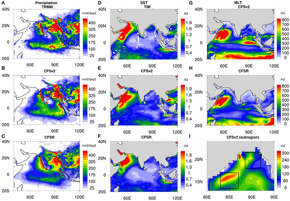
Figure 4. Spatial distribution of daily variances of precipitation (left panel) from (A) TRMM, (B) CFSv2, and (C) CFSR; SST (middle panel) from (D) TRMM, (E) CFSv2, and (F) CFSR. Contour interval is 0.5 (°K)2; MLT (G) CFSv2 and (H) CFSR. The spatial distribution of ML variances over BoB is shown in (I). Solid brown and black boxes in (B) represents the NCEN and BoB regions, and solid black boxes in (I) indicates the northern BoB (17–21°N 88–92°E; NBoB) and southern BoB (12–16°N, 84–87°E; SBoB). MSE budgets are performed over NCEN and BoB and ML budgets are performed over NBoB and SBoB, respectively.

In sharp contrast over the EIO (Figures 3E,F), the observed annual cycles of both SST and precipitation are rather weak. Here, SST is high throughout the annual cycle (>28°C) and considerable rainfall (>4 mm/day) is observed throughout the year with a maximum (>6–8 mm/day) during boreal winter (December–February). In Figures 3G,H, we show the annual cycle of precipitation over land regions and compared with IMD rain gauge and TRMM observations. It is noted that, except in the first week of July over NCEN (Figure 3G), simulated annual cycle exhibits a prominent dry bias over Indian land regions compared to both gauge and satellite observations. The dry bias more intense, when considered continental India (Figure 3H). From, Figure 3H, we also note that the peak in CFsv2 occurs in July and gradually rainfall ceases compared to observations. Duration of seasonal cycle over land regions exhibit, late monsoon “onset” and early “withdrawal in the model simulations. In crux, CFSv2 captures the annual cycle in SST but a wet bias throughout the annual cycle suggesting the sensitivity of model precipitation to surface instability (e.g., Annamalai et al., 2014). In CFSv2 simulations, while the annual cycle of precipitation over a larger monsoon domain (10–30°N, 70–100°E) may be well represented (Sabeerali et al., 2013), an examination of regions relevant to extended monsoon episodes implies model's strengths and weakness.

Subseasonal Properties

Figure 4 shows the spatial distribution of daily variances of precipitation (left panels), SST (middle panels) and MLT (right panels) during boreal summer. Figure 4I shows the MLT only over the BoB region to highlight the small-scale regional differences there (note the different scaling), and caution needs to be done while assessing MLT and SST variations (section Budget Diagnostics). Compared to observed precipitation variance, both in reanalysis and CFSv2 the simulated variance amplitude is weaker (about 18%) and diffused and less coherent along the EIO. Over continental India (NCEN) and BoB (black boxes in Figure 4B; regions where MSE budget diagnostics are performed) spatial coherency in variance pattern is reasonably represented in CFSv2. As regards to SST variance, in response to monsoon winds-induced coastal upwelling, amplitudes of ~2.5 (°K)² are seen along the African coast for both the observations and model simulations (Figures 4D,E) with lesser strength in CFSR (Figure 4F). However, model simulated variance is weaker in amplitude and incoherent in pattern over both the EIO and northern BoB, regions where precipitation variations at extended episodes are of relevance here. Since high temporal resolution MLT observations are still lacking, we compare model-simulated variance with CFSR products (Figures 4G,H). Localized high variances in MLT are collocated with SST variance along the East African coast but CFSv2 simulates erroneously high variance along the eastern EIO without any imprints on the simulated SST variance there (Figure 4E). Further, a careful examination of variance structure over BoB (Figure 4I) indicates large regional differences. i.e., southern BoB is ~280 m² compared to northern region, ~60 m² (thin climatological layer with lesser variance at subseasonal time scales). These differences can impact the SSTs differently and therefore the atmospheric convection at intraseasonal timescales. Next, we examine space-time evolution of variables during extended episodes.

With respect to extended episodes over India, we constructed composite space-time evolution of precipitation, SST and MLT anomalies (Figures 5, 6) and discussed the coherent relationship among them and attempted to identify precursor signals (if any) and validated with TRMM rainfall and TMI SST measurements (Figure not shown). Note, that the number of extended episodes used to prepare the space-time composites are relatively less compared to simulations. Due to lack of space, in the figures, each panel is a 10-day average about the indicated lag; for example, day “0” refers to an average between −5 and +5 days. Budget diagnostics presented later show daily evolution.

FIGURE 5

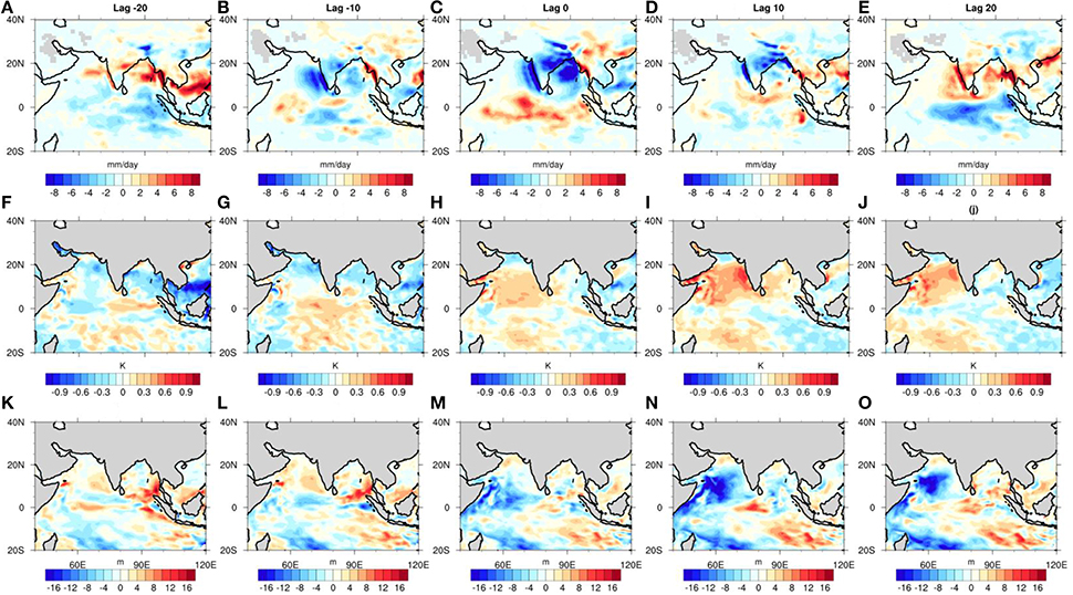
Figure 5. Space-time evolution of composite rainfall anomalies during extended break episodes from CFSv2 simulations. Composite map is shown with lags from −20 to +20 days, where lag “0” represents the peak break phase over the NCEN. The top panels (A–E) show the evolution of rainfall anomalies (mm), the middle panels (F–J) represent the SST (°K) evolution, and the bottom panels (K–O) show MLT (m) anomalies.

FIGURE 6

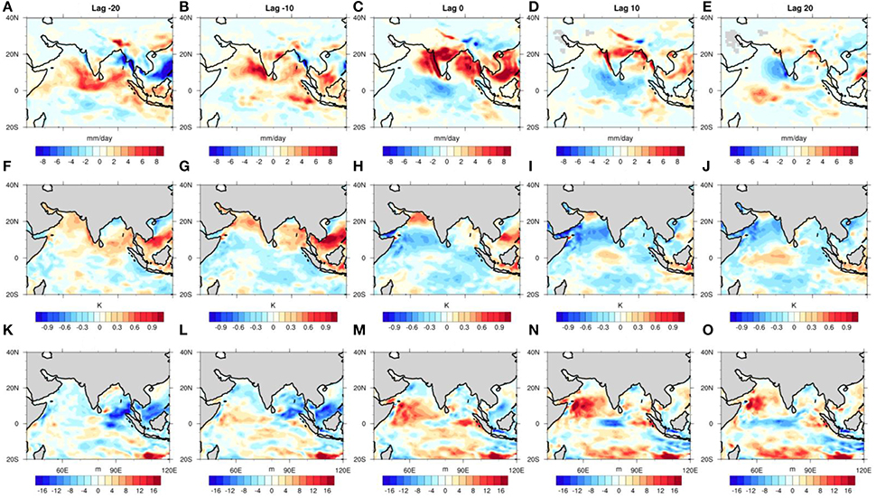
Figure 6. Same as Figure 5, but for extended active composites.

Observed space-time composite, during extended break, exhibits moderate rainfall (~-2 mm/day) anomalies over central Indian region during −20 to −10 days, corresponding SST anomalies exhibit warming (>1 K) over head BoB and northern AS regions. With successive lags negative enhanced rainfall anomalies (>-5 mm/day) extended and covered continental India and BoB. On a similar note, during extended active episodes, observations exhibit initiation of the convective anomalies over EIO at −20 days and progresses poleward in subsequent lags (−10 to 0 days). The enhanced positive rainfall anomalies (>5 mm/day) are seen all over the central India, BoB and extended up to maritime continent (MRC). Observed TMI SST evolution pattern during extended active episodes exhibits warm SST anomalies (>1.5 K) over northern AS and BoB (−20 to −10 days) and with time the anomalies extended spatially into south China Sea and in successive lags (days +10 to +20) SST anomaly pattern becomes negative (~-1.2 K). Overall, the simulated rainfall and SST patterns agrees well with the observations, albeit with certain discrepancies in amplitudes.

Figure 5 shows the composite rainfall evolution (Figures 5A–E), SST (Figures 5F–J), and MLT (Figures 5K–O) during extended break episodes. Rainfall evolution is marked with negative rainfall anomalies (−2 mm/day) over western Indian Ocean at lag −20 days and weak positive rainfall anomalies are over central India and BoB. During this period, negative (positive or deeper) SST (MLT) anomalies ~-0.5 K (>10 m) extend from the northern AS, central and southern BoB all the way to western Pacific (Figures 5F,K). During −10 to 0 days, negative rainfall anomalies amplify and extend diagonally from northwest India to the western Pacific. At −10 days, the negative SST anomalies amplify (~-0.7 K) over the northern BoB (Figure 5G) with signatures of deepened MLT eroding progressively. The composite evolutions indicate that prior to development of suppressed rainfall, oceanic precursor signals exist over the northern BoB. Subsequently, from +10 to +20 days, positive rainfall anomalies from equatorial region gradually move northward and by lag +20 most parts of the Indian landmass and BoB experience enhanced convective activity.

Similarly, in model simulations, during extended active episodes (Figure 6), positive (negative) rainfall anomalies over EIO at −20 days (central India) amplify and propagate poleward (−10 to 0 days) promoting enhanced convection over continental India. Prior to precipitation evolution, shallow MLT and warm SST anomalies cover most parts of northern Indian Ocean extending into South China Sea (−20 to −10 days). Once convection is amplified over south Asia (e.g., day 0), under the influence of strong upwelling-favorable winds, MLT deepens and SST anomalies drop over the AS. Along the EIO, coherent space-time relationship among anomalous precipitation, MLT and SST are less evident, a model limitation.

In summary, lag-lead composites from the model simulations exhibit coherent association among MLT, SST, and precipitation, particularly over the Arabian Sea and BoB. A possible interpretation is that reduced near-surface wind anomalies during extended breaks lead to shallow ML. Furthermore, reduced cloud cover allows more solar radiation to reach the surface, and in conjunction with thin ML warms the sea surface rather rapidly. Compared to observations (Prasanna and Annamalai, 2012) the model simulations switch from extended break (active) to active (break) monsoon episodes rather quickly. Despite these limitations, SST anomalies leading in-situ precipitation anomalies over northern BoB may provide a precursor signal, an issue studied with ML heat budget diagnostic (section Budget Diagnostics).

Although the amplitude of SST anomalies in composites is smaller than observations, certain individual events exhibit SST amplitudes exceeding 1.0° K over northern BoB. Furthermore, about 60–65% of the extended episodes exhibit poleward propagation of precipitation anomalies. On the other hand, an assessment of latitude-time plots for individual years (not shown) suggests that the number of poleward signals originating from the equatorial Indian Ocean and reaching central India is relatively less (1–2 events per year) compared to observations (3–4 events). Additionally, the northward propagation speed ranges from 0.4° to 1.1° day⁻¹, compared to ~1.4° day⁻¹ in observations. Furthermore, the spatial structures of convective anomalies are distorted and the poleward extensions from the equatorial regions are rather limited.

Since one of our goals is to obtain coherent precursor signals in ocean–atmospheric variables, Figure 7 shows the composite time evolution of SST and precipitation over BoB. Day “0” in Figure 7 is the time of maximum rainfall over central India (NCEN). During extended breaks (active) episodes, negative (positive) SST anomalies (red dashed curve) lead in-situ precipitation anomalies (gray solid curve) by 10 days. The model results are consistent with observations (Sengupta and Ravichandran, 2001). The temporal evolution of rainfall anomalies averaged over NCEN (black solid curve) depicts a coherent phase-delay (~5–7 days) with that over BoB during both extended episodes. Thus, monitoring SST, MLT, and precipitation anomalies over BoB may provide lead-time in the prediction of extended monsoon episodes over central India.

FIGURE 7

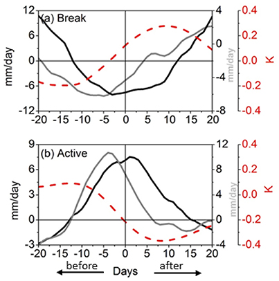
Figure 7. Time evolution of composite SST anomalies (red dashed line) and precipitation anomalies over NCEN (black solid line) and BoB (gray solid line) during extended break (a) and active (b) phases form CFSv2 model simulations. Y-axis with gray and red color denotes the precipitation anomalies and SST anomalies over BoB respectively. Day “0” in the figure represents maximum in precipitation anomalies over NCEN.

Budget Diagnostics

In this section, to identify precursor signals in coupled processes that influence the life cycle extended monsoon episodes, we discuss results of our ML heat and MSE budget analyses. We analyze each individual episode in our solution, as well as their composite. Regarding individual events, we present two cases (each for an extended break and active event, respectively), and highlight “false alarms” in the model simulations that need to be taken into account when looking for precursors. To validate model results, budgets are also performed on events identified with CFSR. First, we present results on ML heat (section ML Heat Budget) followed by MSE diagnostics (section MSE Budget). In the temporal evolution plots shown here (Figures 8–12), day “0” refer to maximum wet (for active) and dry (for break) conditions over the NCEN.

FIGURE 8

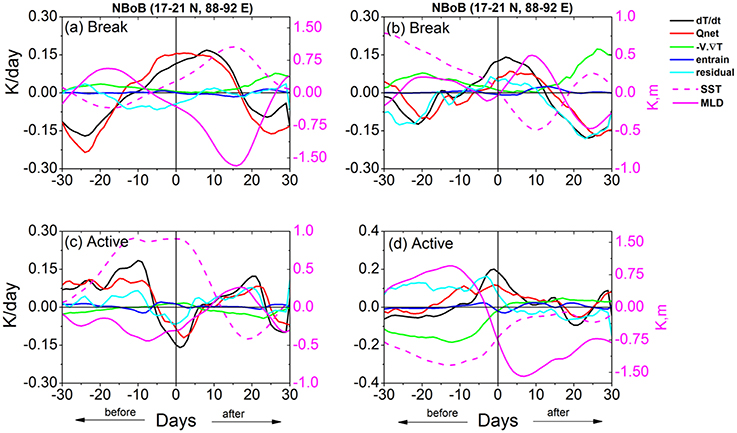
Figure 8. Temporal evolution of various ML heat budget terms, in CFSv2 model solutions, for a typical extended (a) break and (c) active event averaged over NBoB; (b,d) shows inconsistent ML heat budget evolution. For completeness of the budget we have superposed SST (solid magenta line; units in K) and MLT (dashed magenta line; units in m) anomalies. Note, that MLT anomalies scaled to match with SST amplitudes. All other units of the ML budget terms are (°K/day). X-axis represents the time evolution from −30 to +30 days.

ML Heat Budget

Here, our goal is to understand the importance of the terms in (1) in determining SST anomalies. Given that MLT has large regional differences within the BoB (Figure 5I), ML budgets are computed over two regions, namely: (i) the northern BoB (NBoB; 17–21°N, 88–92°E) and (ii) southern BoB (SBoB; 12–16°N, 84–87°E).

Individual Events

Figure 8 shows the temporal evolution of ML budget terms for two sets of individual cases in the NBoB: one set for break episodes (Figures 8a,b) and another for active ones (Figures 8c,d). For completeness, curves for SST and MLT anomalies are also shown. In both the break (Figure 8a) and active (Figure 8c) episodes, MLT and SST variations have an inverse association (compare solid and dashed magenta curves), and Q_net determines the ML heat (SST) tendency throughout the evolution (compare red and black curves). The contributions from advective and entrainment terms are indeed small for SST anomalies. Our interpretations are as follows: Prior to extended break episodes over central India, northern BoB receives moderate positive rainfall anomalies (Figure 5A), enhanced surface wind anomalies (not shown) leading to mixed layer thickening and SST cooling (Figures 5B, 8A). These local thermodynamical conditions are unfavorable to sustain convection, and subsequently precipitation over NBoB reduces (Figure 5B). Thus, reduced cloud cover and enhanced incoming solar radiation increases Q_net. The combination of these effects results in a decrease of MLT and further enhances warm SST anomalies. Under these favorable conditions, SST anomalies gradually become positive and attain maxima (~1° K/day) from 0 to 10 days.

Similarly, during extended active episodes tendency of SST anomalies are also largely influenced by Q_net. Important distinctions between these two cases, however, are the persistence of thin ML for an extended period resulting in the persistence of warm SST anomalies about 15–20 days in the active phase (Figure 8c). One plausible interpretation is that positive precipitation anomalies over NBoB (−10 days onwards, Figure 6B) induce near-surface salinity stratification thinning the ML. An examination of precipitation evolution of this particular event (not shown) indicates enhanced precipitation persistence over NBoB that could further feedback to stratification, thin the ML and warm the sea surface. The phase-lag between anomalous Q_net and SST implies the ocean response time to imposed surface heating or cooling.

In summary, $\frac{dSST}{dt}$ from model simulations are in good agreement with Q_net, indicating the role of air-sea heat fluxes on SST at subseasonal time scales, consistent with observational (e.g., Sengupta and Ravichandran, 2001) and modeling (Shenoi et al., 2002) studies, as well as CFSR results discussed later (Figure 10).

Figures 8b,d show ML heat budget terms from CFSv2 simulations for two individual events that differ markedly. The important distinction in these events is, the inverse relationship between MLT and SST variations is not obvious. For instance, during the break episode from −25 to −15 days, both MLT and SST anomalies are positive. Similarly, during the active episode, from −20 to −10 days, cool SST and deep ML anomalies are seen, rather than warm and thin ones. Note that the magnitudes of advective and residual fluxes are as large as Q_net. This difference suggests that there are individual events, in which the ML budget terms are inconsistent, and at certain times SST anomalies over NBoB could mislead leading to false alarms of extended episodes over central India. Specifically, the persistent negative SST anomalies (Figure 8d) would inform an ensuing extended break.

We must mention here that we examined the ML heat budget for all identified individual extended break and active events and found in break episodes ~60% and in active ones ~65% events depict ML budget evolution realistically.

Composite Budget Analysis

Figure 9 shows the composite evolution of break (top panels) and active (bottom panels) over northern (left panels) and southern (right panels) BoB, and Figure 10 shows the same curves from CFSR. Composites reveal a reasonably good, one-to-one correspondence between $\frac{dSST}{dt}$ and Q_net, and this agreement is more consistent over NBoB than SBoB; also, the contribution of Q_net is relatively large (~70–75%) compared to the other budget terms. Apart from magnitude, the major difference observed between individual events (Figures 8a,c) and composites over the NBoB is the SST-precipitation lead-lag timing. In the composites, SST anomalies leads the peak break (active) phase by ~8 (15) days (Figures 9a,c), whereas it is ~15 (13) days in the individual events (Figures 9a,c). The composite analysis over SBoB also exhibits persistent SST warming before the peak active phase.

FIGURE 9

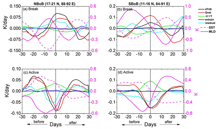
Figure 9. Same as Figure 8, but for composites over NBoB and SBoB.

FIGURE 10

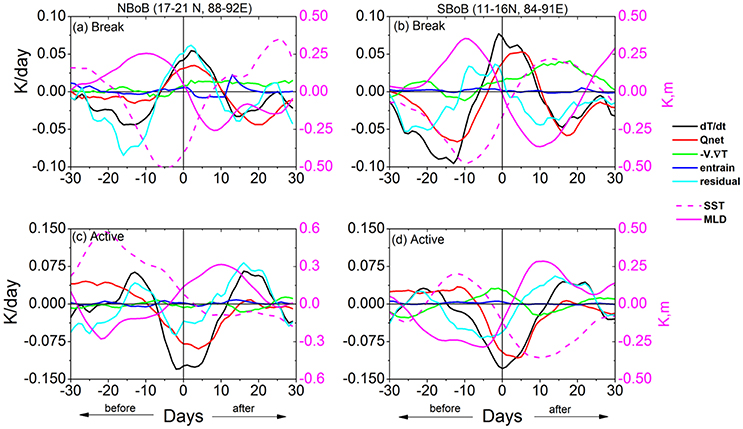
Figure 10. Same as Figure 8, but for ML budget from CFSR data.

Interestingly, residuals with considerable magnitude are found over both the regions contributing SST warming (cooling) during extended break (active) phases. They suggest that there are important terms missing from (1), for example, vertical turbulent mixing, horizontal heat diffusion, etc. Another noticeable feature in the SBoB is the large magnitude of horizontal temperature advection, suggesting that SST changes in the SBoB are also driven by advective fluxes. In the present study, we have not considered the role of ocean currents in the SBoB (e.g., East Indian Coastal Current, EICC) in temperature advection.

The analysis of the ML heat budget using CFSR data (Figure not shown) supports the model results. Specifically, the role of Q_net in priming temperature tendency over NBoB, and the lead-lag association between SST anomalies and monsoon extended events. Akin to CFSv2 diagnostics, the contributions from advective terms over SBoB, and residual terms in both regions are also noticeable in CFSR diagnostics.

MSE Budget

In pursuit of identifying precursor signals in atmospheric processes, as well as processes that are responsible for extended episodes, we performed an MSE budget analysis over the NCEN and BoB. We also expect that these diagnostics could suggest limitations in model physics. Similar to ML heat budgets, we obtain MSE budgets for all individual events and cross-examined them for robustness. Here over NCEN, four individual episodes (two breaks and two active events, Figure 11) and composites (Figure 12) from model solutions. To validate model results, MSE budget is applied to composites constructed from CFSR.

FIGURE 11

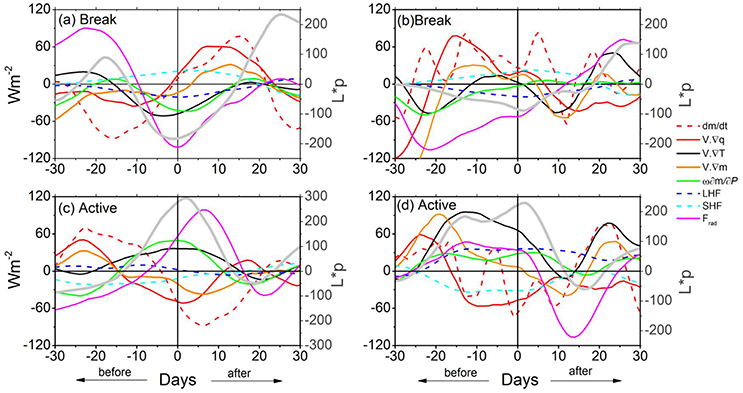
Figure 11. Temporal evolution of various MSE heat budget terms for a typical extended break and active case averaged over NCEN. (a,c) represents the extended break and active phase over NCEN; (b,d) over NCEN for different cases. For completeness of the budget we have superposed precipitation anomalies (L*p, thick solid gray line; units in Wm⁻²). The x-axis represents time evolution from −30 to +30 days.

FIGURE 12

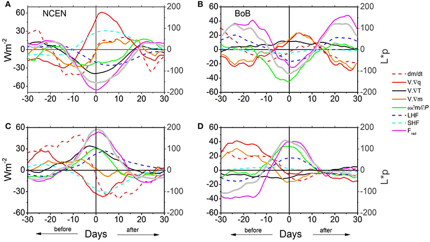
Figure 12. Same as Figure 11, but for the composites during extended monsoon episodes over NCEN and BoB.

Individual Events

Figures 11a,c show the evolution of column-integrated MSE budget terms during a break and active event over NCEN respectively. Analysis indicate, during break episode horizontal moisture advection (−V·∇q), through advecting dry air in the column, leads peak dryness (L*p) by ~12–15 days. Similarly, during an active event, −V·∇q leads the peak wetness (L*p) by about 20 days. Note that this term is the main contributor to the charging and discharging of MSE anomalies ($\frac{dm}{dt}$) during both episodes. Akin to persistence of warm SST anomalies over NBoB during extended active episodes (Figure 8c), column MSE charging shows persistence character (or slow rate of discharging from −25 to −10 days) with contributions from horizontal temperature advection (−V·∇T), and vertical advection of MSE ($\omega \frac{\partial m}{\partial p}$), respectively. As expected in tropics, L*p and $\omega \frac{\partial m}{\partial p}$ show coherent relationship during both episodes. The net radiative flux divergence (F_rad) along with contributions from −V·∇T promotes maintenance of extended episodes. Contributions from surface-flux anomalies are rather marginal. Note that F_rad is a consequence of convection, and appears to be an efficient feedback term in prolonging the active and break events over central India (cf. Prasanna and Annamalai, 2012).

To summarize, horizontal advection of moisture acts as the leading MSE term in drying (moistening) the atmosphere prior to extended break (active) phases, and column net radiative flux divergence is a key diabatic source term in maintaining them. One commonality between the two events is the substantial contribution from horizontal temperature advection. It could be due to model deficiency in capturing the physical processes associated with the physical parameterization schemes. Exploring the reasons for this aspect is deferred to a companion work (manuscript in preparation).

Figures 11b,d show the MSE budgets for another case of typical extended break and active events over NCEN. Comparing them to the left panels (Figures 11a,c), the precursor signals in −V·∇q, and the role of F_rad in maintenance of the episodes are not clear. Moreover, high-frequency variations of $\frac{dm}{dt}$ anomalies imply lack of gradual charging and discharging of MSE anomalies. Finally, contributions from −V·∇T, particularly during active episode are too large. Similar to errors leading to false alarms in ML heat terms discussed earlier, before a break (active) event horizontal advection of moist (dry) air in MSE budgets does raise a false alarm.

Composite Budget Analysis

Figure 12 shows the model composite budget evolution over NCEN (Figures 12A,C) and BoB (Figures 12B,D).

Broadly, our composite MSE budget results also exhibits the precursor signals in −V·∇q, and the role of F_rad and −V·∇T in maintenance of the extended episodes. Model results agree with those of CFSR (Figure not shown). However, compared to individual events contributions from surface fluxes (LHF and SHF) and −V·∇T are stronger in the model composite evolution. While one plausible attribute to this may come from “false alarm” events such as those presented in Figures 11B,D that also have similar contributions, large surface flux terms in budgets could be due to misrepresentations of model short and longwave radiation terms, boundary layer parameterization processes. On a similar note large temperature advection in (Figures 12A,C) shows the misrepresentations of model temperature and/or advection term (physics and dynamical core).

Given the fact that precipitation anomalies over the NBoB precede that over NCEN, and that anomalies SST over NBoB serve as a precursor (Figure 7), we also examined the MSE budget diagnostics over NBoB to assess the robustness to that over NCEN. Over the open oceans of the BoB (Figures 12B,D) break (active) event in the model is clearly preceded by an active (break) event (see also Figures 5, 6). Unlike in other plots, here “day 0” corresponds to peak dry or wet conditions over BoB. The dominance contributions of −V·∇q in initiating and F_rad in maintaining the extended events are robust features, with relatively long lead timings in −V·∇q in both the episodes. Unlike contributions from −V·∇T over NCEN, latent heat flux (LHF) anomalies provide additional column MSE in events maintenance over NBoB. However, model diagnostics differ considerably with CFSR results (Figure not shown), particularly in the lead timings of −V·∇q, and relative contributions from −V·∇T and $\omega \frac{\partial m}{\partial p}$ in the budget evolutions. These differences are perhaps due to the different physical parameterizations and tuning parameters in CFSR and CFSv2 model solutions. Broadly, processes based diagnostics applied here has direct linkages to model parameterization schemes. For example, vertically integrated moist static energy (MSE) budget provides information about vertical advection of moisture and MSE (vertical profile of vertical velocity depends on model cumulus parameterization), free troposphere moisture variations are associated with moisture-convection feedbacks, and net radiative flux divergence implies cloud-radiative feedbacks. Given that monsoon region is data sparse and model prejudices influence reanalysis thermodynamical variables, results from CFSR too need to be verified with sustained observations. Overall, our budget analysis, consistent with the earlier works (Prasanna and Annamalai, 2012; Hanf et al., 2017; Mohan and Annamalai, under review), provide robustness in precursor signals and false alarms in key ocean and atmospheric variables during the evolution of extended monsoon episodes.

Source of Dryness and Moistening

Earlier by diagnosing reanalysis products, Prasanna and Annamalai (2012) and Mohan and Annamalai, (under review), by decomposing the advection term (−V·∇q) into its mean and perturbation components (equation 3), identified that for extended breaks (active events) the source of dry (moist) air originates in West African desert regions (near-equatorial Indian Ocean) with the level of maximum dryness (wetness) centered near 600 hPa. A similar investigation on CFSv2 solutions suggests that anomalous winds advecting climatological moisture gradient (–V′·∇q^o) with origins over northern Arabian continent is the dominant source of dry air prior to extended breaks over NCEN, and that the climatological winds acting on anomalous moisture gradient (V^o·∇q′) with origin over western Arabian Sea is the source of moist air prior to extended active episodes over NCEN (figures not shown).

Summary and Discussion

Summary

In this study, we analyze 30 years of output from a freely coupled CFSv2 solution to assess model's capability to simulate extended (>7 days), active and break monsoon episodes during boreal summer over continental India. Since CFSv2 is employed for real-time prediction of monsoon over South Asia, for individual and composite events we apply process-based diagnostics such as vertically integrated MSE budget and ML heat budget to identify precursor signals in both ocean and atmospheric variables, and also to identify any false alarms. Keeping in mind that CFSv2 is employed for operational monsoon predictions, a detailed examination of processes carried out here provides not only robust precursor signals but also highlights model's strengths and weakness, and suggest pathways for future model development.

Our examination of model's fidelity in simulating the monsoon basic state (section Basic State and Intraseasonal Variability) suggests that CFSv2, like most coupled models, depict large systematic biases in variables important for ocean-atmosphere interactions. Nevertheless, one of the major strength is, model integrations capture many aspects of monsoon extended break and active episodes realistically encouraging us to apply process-based diagnostics.

While ML heat budgets for individual episodes as well as composites examined over the NBoB suggest that anomalous SST warming, and cooling are largely governed by Q_net. Specifically, mixed-layer temperature tendency term $\left(\frac{dSST}{dt}\right)$ from model simulations are in phase with Q_net, indicating the role of air-sea heat fluxes on SST at subseasonal time scales, consistent with earlier studies (e.g., Sengupta and Ravichandran, 2001; Shenoi et al., 2002), as well as in CFSR results. However, a major drawback in ML budgets is the inverse relationship between SST and MLT. As, seen from Figures 8b,d, at certain times SST anomalies over NBoB could mislead, leading to false alarms. These errors, in particular influence air-sea fluxes at sub-seasonal time scales could possibly affect mean state through feedback processes. Throughout the life cycle of extended episodes, cool (warm) SST anomalies associated with extended break (active) events precede in-situ precipitation anomalies by 10–14 days. A major difference between the two episodes is the persistence of warm SST anomalies prior to extended active events (Figures 8, 9).

While the composite analysis of the column-integrated MSE budgets show −V·∇q is the leading MSE term (~15 days) in initiating, net radiative flux divergence in maintaining, the extended monsoon episodes, with surface fluxes playing a secondary role, there are certain individual events, in which the leading MSE budget terms misrepresent the evolution and inconsistency between vertical advection of MSE and precipitation anomalies (L*p) exist (Figures 12C,D). Within the model caveat (in representing the extended active events, Figure 1A), both budget diagnostics provide model's capability in identifying the leading terms. However, extreme caution needs to be exercised while interpreting the model real-time forecasts for extended active monsoon conditions.

An investigation of individual terms of moisture advection (Equation 3) on CFSv2 solutions suggests that anomalous winds advecting climatological moisture gradient (–V′·∇q^o) with origins over northern Arabian continent is the dominant source of dry air prior to extended breaks over NCEN, and that the climatological winds acting on anomalous moisture gradient (V^o·∇q′) with origin over western Arabian Sea is the source of moist air prior to extended active episodes over NCEN (figures not shown). One model limitation is that in reanalysis diagnostics the horizontal advection of dry air could be traced back to the African desert regions (Mohan and Annamalai, under review).

The coupled nature of these precursors can be summarized as follows: Beginning from the precursory signal prior to extended breaks, the accumulation of dry air in mid-troposphere inhibits vertical growth of convection and results in enhanced radiative cooling that then maintains the break conditions. During the evolution of extended break, due to reduced near-surface winds ML thins, and in conjunction with clear-sky conditions, SST warms over the Arabian Sea first and then over the and Bay of Bengal. Subsequently, the atmosphere-to-ocean fluxes are increased, and warm SST anomalies persist and amplify, and subsequently favor convection and monsoon active phase is initiated over the Bay of Bengal. The active monsoon conditions then induce stronger near-surface winds that promote deepening of ML and emergence of cold SST anomalies. The development of cold SST anomalies is further anchored by reduced incoming solar radiation reaching the surface. This coupled ocean-atmosphere interaction then sets the conditions for the ensuing breaks. Model solutions clearly indicate that prior to extended breaks, prolonged active conditions prevail over the NBoB (Figure 12B).

In summary, SST variations over the NBoB suggest that SST anomalies lead precipitation anomalies by about 8 (10) days during active (break) episodes (Figure 7). From the atmospheric point of view, the MSE budgets reveal moisture advection to be a coherent precursor signal (~10 days). The lead times of the precursor signals (moisture and SST anomalies) obtained from the MSE and ML budget diagnostics will be of potential use for modeling community to monitor and prediction of these extended monsoon episodes.

Discussion

Over the past few decades, sustained research from observations, models, and theory have led to a consensus that monsoons arise due to complex interactions among ocean, atmosphere and land components of the climate system. As such, the amount of precipitation during the summer (June–September) monsoon has huge socio-economic impacts in the region, and accurate rainfall forecasts on time scales of days-to-seasons are of critical importance. Despite the recognition of the societal need, skill in monsoon prediction over South Asia by dynamical climate models remains low. The low skill is perhaps due to model errors or biases in simulating the annual cycle of the monsoon (Sperber et al., 2013). Results presented here and elsewhere clearly show the persistent systematic errors in CFSv2 basic state over the monsoon-tropical Indian Ocean climate systems, indicate considerable change in the air-sea interactions and resultant ocean and atmosphere budgets. In terms of atmospheric precursor signals identified here, anomalous winds advecting climatological moisture gradient (V′·∇q^o) with origins over northern Arabian continent is the dominant source of dry air prior to extended breaks over NCEN, and that the climatological winds acting on anomalous moisture gradient (V^o·∇q′) with origin over western Arabian Sea is the source of moist air prior to extended active episodes over NCEN (figures not shown), suggesting that forecast models must realistically represent the climatological distribution of moisture and circulation fields during the season for better prediction.

To what degree, model identified “false alarms” in extended monsoon episodes are due to these systematic errors? We showed that in certain individual events, both the ML heat and MSE budgets show incoherent relationships among budget terms. More importantly, results from Figure 8b indicate that during the break episode from −25 to −15 days, both MLT and SST anomalies are positive. Similarly, during the active episode (Figure 8d), from −20 to −10 days, cool SST and deep ML anomalies are seen, rather than warm and thin ones. While, the persistent SST warming or cooling in ML budgets is largely governed by net heat flux (Figures 8, 9), in “false alarm” events, the robust relationship between surface fluxes and SST variations are not represented well. Implies the flux terms (either heat flux or advective fluxes) does not account for any variations in either SST warming or cooling tendencies. Specifically, the persistent negative SST anomalies (Figure 8d) would inform an ensuing extended break. Thus, model SST anomalies over NBoB could mislead to false alarms of extended episodes over central India. An investigation into their causes is beyond the scope here but indicates that care must be taken while interpreting the budget diagnostics, since this model is employed for operational prediction. We also noted similar false alarms in the examination of MSE budgets for individual events (Figures 11b,d), which indicate the inconsistency in model's cumulus parameterization and free tropospheric moisture variations associated with moisture-convection feedback mechanisms. In summary, we note that for about 1/3 of the identified extended break and active episodes, inconsistencies in budget diagnostics suggest identified precursor signals could lead to false alarms. Apart from false alarms, compared to observations, CFSv2 systematically simulates a greater number of extended monsoon active episodes.

Future work will identify the source of model systematic errors in the coupled basic state of the monsoon-tropical Indian Ocean system and investigate possible reasons for budget inconsistencies in certain individual events. To constrain model physics, however, in-situ sustained observations over the monsoon regions are needed.

Author Contributions

MT-Contributed in analyzing the CFSv2 data, diagnostics and preparing the manuscript. HA-Contributed in interpretation of the results and preparing the manuscript. LM-Contributed in providing the comments and suggestions in the preparation of the manuscript. BH-Contributed in providing the comments and suggestions in the preparation of the manuscript. JK-Contributed in providing the comments and suggestions in the preparation of the manuscript.

Conflict of Interest Statement

The authors declare that the research was conducted in the absence of any commercial or financial relationships that could be construed as a potential conflict of interest.

Acknowledgments

HA and TM sincerely acknowledge the support from the Ministry of Earth Sciences (MoES), Government of India, as part of the Monsoon Mission Project to carry out this research. Dr. McCreary read the draft version of the manuscript and provided valuable comments and suggestions. The authors would like to thank the Editor and two reviewers for their valuable comments that have helped improve the manuscript.

References

Abhik, S., Mukhopadhyay, P., Krishna, R. P., Kiran Salunke, M., Ashish Dhakate, D., Suryachandra, R., et al. (2016). Diagnosis of boreal summer intraseasonal oscillation in high resolution NCEP climate forecast system. Clim. Dyn. 46, 3287. doi: 10.1007/s00382-015-2769-9

CrossRef Full Text | Google Scholar

Annamalai, H. (2010). Moist dynamical linkage between the equatorial Indian Ocean and the south Asian monsoon trough. J. Atmos. Sci. 67, 589–610. doi: 10.1175/2009JAS2991.1

CrossRef Full Text | Google Scholar

Annamalai, H., Hafner, J., Kumar, A., and Wang, H. (2014). A Framework for dynamical seasonal prediction of precipitation over the Pacific Islands. Climate J. 27, 3272–3297. doi: 10.1175/JCLI-D-13-00379.1

CrossRef Full Text | Google Scholar

Annamalai, H., Hamilton, K., and Sperber, K. R. (2007). South Asian summer Monsoon and its relationship with ENSO in the IPCC AR4 simulations. J. Climate 20, 1071–1092. doi: 10.1175/JCLI4035.1

CrossRef Full Text | Google Scholar

Annamalai, H., Taguchi, B., McCreary, J. P., Nagura, M., and Miyama, T. (2017). Systematic errors in South Asian monsoon simulation: importance of equatorial indian ocean processes. J. Climate 30, 8159–8178. doi: 10.1175/JCLI-D-16-0573.1

CrossRef Full Text | Google Scholar

Bhat, G., Gadgil, S., Hareesh Kumar, P. V., Kalsi, S. R., Madhusoodanan, P., Murty, V. S. N., et al. (2001). BOBMEX—The Bay Of Bengal Monsoon Experiment. Bull. Am. Meteorol. Soc. 82, 2217–2243. doi: 10.1175/1520-0477(2001)082<2217:BTBOBM>2.3.CO;2

CrossRef Full Text | Google Scholar

Chaudhari, H. S., Pokhrel, S., Mohanty, S., and Saha, S. K. (2013). Seasonal prediction of Indian summer monsoon in NCEP coupled and uncoupled model. Theo. Appl. Clim. 114, 459–477. doi: 10.1007/s00704-013-0854-8

CrossRef Full Text | Google Scholar

Duvel, J. P., and Vialard, J. (2007). Indo-Pacific sea surface temperature perturbations associated with intraseasonal oscillations of tropical convection. J. Clim. 20, 3056–3082. doi: 10.1175/JCLI4144.1

CrossRef Full Text | Google Scholar

Ek, M., Mitchell, K. E., Lin, Y., Rogers, E., Grunmann, P., Koren, V., et al. (2003). Implementation of Noah land-surface model advances in the NCEP operational mesoscale Eta model. J. Geophys. Res. 108:8851. doi: 10.1029/2002JD003296

CrossRef Full Text

Fu, X., Wang, B., Li, T., and McCreary, J. P. (2003). Coupling between northward-propagating intraseasonal oscillations and sea-surface temperature in the Indian Ocean. J. Atmos. Sci. 60, 1733–1753. doi: 10.1175/1520-0469(2003)060<1733:CBNIOA>2.0.CO;2

CrossRef Full Text | Google Scholar

Goswami, B. B., Deshpande, M., Mukhopadhyay, P., Subodh, K. S., Suryachandra Rao, A., Raghu, M., et al. (2014). Simulation of monsoon intraseasonal. variability in NCEP CFSv2 and its role on systematic bias. Clim. Dyn. 43, 2725–2745. doi: 10.1007/s00382-014-2089-5

CrossRef Full Text | Google Scholar

Griffies, S. M., Harrison, M. J., Pacanowski, R. C., and Rosati, A. (2004). A Technical Guide to MOM4. NOAA/Geophysical Fluid Dynamics Laboratory, 337.

Hanf, F. S., Annamalai, H., Rinke, A., and Dethloff, K. (2017). South Asian summer monsoon breaks: process-based diagnostics in HIRHAM5. J. Geophys. Res. Atmos. 122, 4880–4902. doi: 10.1002/2016JD025967

CrossRef Full Text | Google Scholar

Holte, J., and Talley, L. (2009). A new algorithm for finding mixed layer depths with applications to Argo data and subantarctic mode water formation. J. Atm. Oceanic Tech. 26, 1920–1939. doi: 10.1175/2009JTECHO543.1

CrossRef Full Text | Google Scholar

Huffman, G. J., Adler, R. F., Bolvin, D. T., Gu, G., Nelkin, E. J., Bowman, K. P., et al. (2007). The TRMM Multisatellite precipitation analysis: Quasi global, multi-year, combined sensor precipitation estimates at fine scale. J. Hydrometeor. 8, 38–55. doi: 10.1175/JHM560.1

CrossRef Full Text | Google Scholar

Kim, H.-M., Webster, P. J., and Curry, J. A. (2012). Seasonal prediction skill of ECMWF System 4 and NCEP CFSv2 retrospective forecast for the Northern Hemisphere Winter. Clim. Dyn. 39, 2957–2973. doi: 10.1007/s00382-012-1364-6

CrossRef Full Text | Google Scholar

Levine, R. C., Turner, A. G., Marathayil, D., and Martin, G. M. (2013). The role of northern Arabian Sea surface temperature biases in CMIP5 model simulations and future projections of Indian summer monsoon rainfall Clim. Dyn. 41, 155–172. doi: 10.1007/s00382-012-1656-x

CrossRef Full Text | Google Scholar

Maloney, E. D. (2009). The moist static energy budget of a composite tropical intraseasonal oscillation in a climate model. Climate J. 22, 711–729. doi: 10.1175/2008JCLI2542.1

CrossRef Full Text | Google Scholar

McCreary, J. P., Kundu, P. K., and Molinari, R. L. (1993). A numerical investigation of the dynamics, thermodynamics and mixed-layer processes in the Indian Ocean. Prog. Oceanogr. 31, 181–244. doi: 10.1016/0079-6611(93)90002-U

CrossRef Full Text | Google Scholar

Nagura, M., McCreary, J. P., and Annamalai, H. (2017). Origins of coupled-model biases in the Arabian-Sea climatological state. Climate J. doi: 10.1175/JCLI-D-17-0417.1

CrossRef Full Text | Google Scholar

Neelin, J. D., and Held, I. M. (1987). Modeling tropical convergence based on the moist static energy budget. Mon. Weather Rev. 115, 3–12. doi: 10.1175/1520-0493(1987)115<0003:MTCBOT>2.0.CO;2

CrossRef Full Text | Google Scholar

Neelin, J. D., and Su, H. (2005). Moist teleconnection mechanisms for the tropical South American and Atlantic sector. Climate J. 18, 3928–3950, doi: 10.1175/JCLI3517.1

CrossRef Full Text | Google Scholar

Prasanna, V., and Annamalai, H. (2012). Moist dynamics of extended monsoon breaks over south Asia. Climate J. 25, 3810–3831, doi: 10.1175/JCLI-D-11-00459.1

CrossRef Full Text | Google Scholar

Sabeerali, C. T., Ramu Dandi, A., Dhakate, A., Salunke, K., Mahapatra, S., and Rao, S. A. (2013). Simulation of boreal summer intraseasonal oscillations in the latest CMIP5 coupled GCMs. J. Geophys. Res. Atmos. 118, 4401–4420. doi: 10.1002/jgrd.50403

CrossRef Full Text | Google Scholar

Saha, S., Moorthi, S., Wu, X., Wang, J., Nadiga, S., Tripp, P., et al. (2014). The NCEP climate forecast system version 2. Clim. J. 27, 2185–2208. doi: 10.1175/JCLI-D-12-00823.1

CrossRef Full Text | Google Scholar

Saha, S. K., Pokhrel, S., Chaudhari, H. S., Dhakate, A., Shewale, S., Sabeerali, C. T., et al. (2014). Improved simulation of Indian summer monsoon in latest NCEP climate forecast system free run. Int. J. Climatol. 34, 1628–1641. doi: 10.1002/joc.3791

CrossRef Full Text | Google Scholar

Saha, S., Moorthi, S., Pan, H.-L., Wu, X., Wang, J., Nadiga, S., et al. (2010). The NCEP climate forecast system. J. Clim. 19, 3483–3517. doi: 10.1175/JCLI3812.1

CrossRef Full Text

Sengupta, D., Goswami, B. N., and Senan, R. (2001). Coherent intraseasonal oscillations of ocean and atmosphere during the Asian summer monsoon. Geo. phys. Res. Lett. 28, 4127–4130. doi: 10.1029/2001GL013587

CrossRef Full Text | Google Scholar

Sengupta, D., and Ravichandran, M. (2001). Oscillations of Bay of Bengal sea surface temperature during the 1998 summer monsoon. Geo. phys. Res. Lett. 28, 2033–2036. doi: 10.1029/2000GL012548

CrossRef Full Text | Google Scholar

Sharmila, S., Pillai, P. A., Joseph, S., Roxy, M., Krishna, R. P. M., Chattopadhyay, R., et al. (2013). Role of ocean-atmosphere interaction on northward propagation of Indian summer monsoon intra-seasonal oscillations (MISO). Clim. Dyn. 41, 1651–1669. doi: 10.1007/s00382-013-1854-1

CrossRef Full Text | Google Scholar

Shenoi, S. S. C., Shankar, D., and Shetye, S. R. (2002). Differences in heat budgets of the near-surface Arabian Sea and Bay of Bengal: implications for the summer monsoon. J. Geophys. Res. 107, 5-1–5-14. doi: 10.1029/2000JC000679

CrossRef Full Text | Google Scholar

Shukla, R. P., and Huang, B. (2016). Mean state and interannual variability of the Indian summer monsoon simulation by NCEP CFSv2. Clim. Dyn. 46:3845. doi: 10.1007/s00382-015-2808-6

CrossRef Full Text | Google Scholar

Shukla, R. P., and Zhu, J. (2014). Simulations of boreal summer intraseasonal Oscillations with the climate forecast system, version 2, over India and the Western Pacific: role of air–sea coupling. Atmosphere Ocean 52, 321–330. doi: 10.1080/07055900.2014.939575

CrossRef Full Text | Google Scholar

Sikka, D. R., and Gadgil, S. (1980). On the maximum cloud zone and the ITCZ over India longitude during the Southwest monsoon. Mon. Weather Rev. 108, 1840–1853. doi: 10.1175/1520-0493(1980)108<1840:OTMCZA>2.0.CO;2

CrossRef Full Text | Google Scholar

Sperber, K. R., Annamalai, H., Kang, I.-S., Kitoh, A., Moise, A., Turner, A., et al. (2013). The Asian summer monsoon: an intercomparison of CMIP5 vs. CMIP3 simulations of the late 20th century. Clim. Dyn. 41, 2711–2744. doi: 10.1007/s00382-012-1607-6

CrossRef Full Text | Google Scholar

Sperber, K. R., and Palmer, T. N. (1994). Interannual tropical rainfall variability in general circulation model simulations associated with the atmospheric model intercomparision project. J.Clim. 9, 2727–2750. doi: 10.1175/1520-0442(1996)009<2727:ITRVIG>2.0.CO;2

CrossRef Full Text

Turner, A. G., Inness, P. M., and Slingo, J. M. (2005). The role of the basic state in the ENSO-monsoon relationship and implications for predictability. Q. J. R. Meteorol. Soc. 131, 781–804. doi: 10.1256/qj.04.70

CrossRef Full Text | Google Scholar

Vialard, J. (2012). Ocean-Atmosphere Variability over the Indo-Pacific Basin. Ocean, Atmo-Sphere. Universit e Pierre et Marie Curie-Paris, VI, 2009.

Yasunari, T. (1979). Cloudiness fluctuations associated with the northern hemisphere summer monsoon. J. Meteor. Soc. Jap. 57, 227–242. doi: 10.2151/jmsj1965.57.3_227

CrossRef Full Text | Google Scholar