ROPES Reveals Past Land Cover and PPEs From Single Pollen Records

Objectives

The field of pollen analysis was established 100 years ago, following the presentation of first pollen diagrams by Swedish geologist Lennart von Post (von Post, 1918). Initially used for stratigraphic purposes, the power of pollen analysis to reconstruct past landcover was soon recognized—and it has remained the most powerful tool in that field until today. Reconstructing past landcover from the pollen record is far from simple, however. The most obvious limitations arise from the production bias and the dispersal bias: pollen productivity as well as pollen dispersal differ among plant taxa. Moreover, pollen deposition at each site is composed of pollen arriving from the vicinity of the sample site as well as of pollen arriving from farther away. Because nearby pollen sources contribute more pollen than distant ones, the pollen record represents the surrounding vegetation in a distance weighted manner.

Despite the long history of the field, quantitative methods to correct for these biases only came into regular use over the past decade. The most widespread approach is the REVEALS model (Regional Estimates of VEgetation Abundance from Large Sites, Sugita, 2007), which aims to translate pollen deposition from large lakes into regional vegetation composition. REVEALS is a correction factor approach; it employs pollen productivity estimates (PPEs) to correct for the production bias and models of pollen dispersal to correct for the dispersal bias in pollen data. PPEs so far derive from calibration studies that relate present day vegetation to modern pollen deposition across a series of sites. Calibration of such surface sample PPEs is cumbersome: it requires pollen data from multiple sites, plant abundances in the pollen source area of each site and a profound understanding of pollen dispersal and deposition. The surface sample PPEs are then applied in palaeo-reconstructions under the assumption that pollen productivity of plant taxa in the past equals present day productivity. This assumption may often be violated, however, because pollen productivity is influenced by climate (Hicks, 1999), stand structure (Matthias et al., 2012; Feeser and Dörfler, 2014) or land management (Theuerkauf et al., 2015). Furthermore, for pollen morphotypes that include numerous taxa, natural or human induced changes in actual species composition may alter overall pollen productivity. This effect is most obvious for grasses, because pollen productivity differs significantly between the various species (Prieto-Baena et al., 2003). The use of PPEs based on (modern) surface sample studies therefore introduces a yet unknown error in REVEALS applications. In addition, because REVEALS produces proportional abundances, error in the PPE of just one taxon will introduce error in the reconstructed cover of all taxa in the record.

Already von Post (1918) recognized that absolute pollen data, i.e. pollen accumulation rates (PAR), potentially provide an independent record for each taxon, devoid of such mutual disturbances. Yet, calculating PARs requires exact chronologies and so only became feasible with radiocarbon dating in the 1960s. Early applications showed that PAR values can be very noisy, however; even across a single lake they may differ by orders of magnitude due to sediment redeposition and focusing (Davis, 1967). These results raised much skepticism against the usability of PARs to quantify past abundances so that the field was largely abandoned, with the exception of treeline studies. Across treelines, changes in PAR values are large compared to the noise so that they have been proven a useful tool (Hicks, 2001; Seppä and Hicks, 2006; Theuerkauf and Joosten, 2012). Giesecke and Fontana (2008) have demonstrated that the noise in PAR data can be reduced with careful site selection. The question arises whether and how PAR values can be used in a sensible and robust way in quantitative vegetation reconstruction. We here suggest the ROPES approach (REVEALS withOut PpES), which combines PAR values with the REVEALS model in an optimization algorithm. The main underlying idea is that not the PAR values as such, but changes in the PAR values are meaningful and robust.

Validation

The Principle of ROPES

ROPES derives from two main assumptions: (i) the REVEALS model allows to translate pollen counts from large lakes into past regional plant abundances and (ii) for each taxon, absolute pollen deposition at a site is a linear representation of its distance weighted abundance (Prentice and Webb, 1986). Hence, changes in abundance result in similar changes in pollen deposition. For example, if the abundance of pine around a site has doubled at some time in the past, then also deposition of pine pollen at that site has doubled. Because of the production and dispersal bias in pollen data, such a linear relationship does not exist for proportional (percentage) pollen data. If the abundance of pine doubles, the change in percentage values can be very different, depending on overall vegetation composition. Correction with REVEALS would reconstruct a doubling in pine abundance in accordance with a doubling in pollen deposition. However, correction will only be accurate with appropriate parameters, including PPEs. We suggest that this relationship can be used to test the performance of REVEALS applications with PAR data: each change in abundances reconstructed with REVEALS should correspond to similar changes in PAR values. Moreover, we can use this relationship to apply REVEALS without predefined PPEs. To that end we suggest the ROPES approach.

We illustrate the approach using just two samples and two taxa, A and B (Table S1). For both samples, PAR and percentage values are known: the PAR value of A increases from 1,000 to 2,000 grains cm⁻² year⁻¹ from sample 2 to sample 1, the PAR value of B decreases from 800 to 600 grains cm⁻² year⁻¹. The pollen percentages of A increase from 55.8 to 76.9% while those of B decrease from 44.4 to 23.1%.

We do not know pollen productivity (or PPEs) of A and B—so we apparently cannot apply REVEALS to reconstruct the actual abundances. Still, from the PAR values we can infer that the abundance of A has doubled from sample 2 to sample 1, while the abundance of B declined by 25%. We now argue that a REVEALS reconstruction should show the same trends in both taxa: a doubling in A and a 25% decline in B. With that premise, we can try and find PPEs that produce this pattern. Let us use B as the reference taxon, i.e., the PPE of B = 1. For taxon A we apply REVEALS with different PPEs: 1, 2, 3,…, 10. Only with a PPE of A = 5, REVEALS produces the expected changes: a doubling in A and a 25% decline in B. Correspondingly, the ratio of PAR values to reconstructed abundance (PAR over REVEALS, or PoR ratio) is constant for both taxa, 50 for A and 10 for B, because reconstructed abundance is linearly represented in the PAR values. We now know that the PPE of A is 5 (with that of B set to 1), and that the abundance of taxon A increased from 20% to 40% while that of B declined from 80 to 60%.

To summarize, ROPES assumes that a REVEALS reconstruction is correct only if changes in the reconstructed abundance of each taxon are proportional to changes in the respective PAR values. To find PPEs that produce such a reconstruction, ROPES applies an optimization algorithm that minimizes variation in the PoR ratio between samples by adjusting initially random PPEs. After optimization, the PoR ratio will (in absence of noise) be constant along the record. In the end, ROPES simultaneously calculates mean plant abundances and PPEs.

Assumptions of ROPES

As the REVEALS model is an integral part of the ROPES approach, ROPES inherently assumes that the assumptions underlying the REVEALS model (Sugita, 2007) are valid. ROPES finds suitable PPEs and plant abundances by minimizing variation in the PoR ratio. However, this ratio is expected to be constant only under certain conditions, as we outline below. For each taxon i, the PoR ratio along a pollen record is calculated as the PAR value divided by the cover reconstructed with the REVEALS model:

$\begin{array}{rc}{PoR}_i=\frac{PA{R}_i}{Reconstructedabundanceofi}& (1)\end{array}$

It is a general assumption in palynology that in a basin pollen deposition of taxon i, here expressed as PAR values, is a function of absolute pollen productivity of i [P_i], the abundance of i as a function of distance z [X_i(z)] and the pollen dispersal and deposition function [g_i(z)] integrated over distance Z _max starting from the edge of the basin with radius R (cf. Sugita, 2007):

$\begin{array}{rc}PA{R}_i=P_i·{\displaystyle \underset{R}{\overset{Z_{max}}{\int }}}{X}_i(z)·g_i(z)·dz& (2)\end{array}$

Sugita (2007) argues that for large lakes in a homogeneous landscape, X_i(z) equals mean regional abundance $\overline{X}$ of taxon i:

$\begin{array}{rc}PA{R}_i=P_i·{\displaystyle \underset{R}{\overset{Z_{max}}{\int }}}{\overline{X}}_i·g_i(z)·dz& (3)\end{array}$

In the REVEALS model (Sugita, 2007) the integral over the dispersal and deposition function g_i(z) is expressed as the K factor:

$\begin{array}{rc}PA{R}_i=P_i·{\overline{X}}_i·K_i& (4)\end{array}$

REVEALS produces the reconstructed abundances as proportion of total regional abundances, or the total area A represented in the pollen record (i.e. the sum of all X_i):

$\begin{array}{rc}Reconstructedabundanceofi=\frac{{\overline{X}}_i}{A}& (5)\end{array}$

In result, the PoR ratio of taxon i is the absolute pollen productivity of taxon i multiplied with dispersal factor K_i and the total area A represented in the pollen record:

$\begin{array}{rc}Po{R}_i=P_i·K_i·A& (6)\end{array}$

The final equation shows that the PoR ratio is constant along a record if three conditions are fulfilled: (i) pollen productivity is constant over time, (ii) pollen dispersal and deposition processes remained unchanged, and (iii) the area represented in the pollen record is stable. We illustrate and discuss how changes in pollen productivity and in the total area affect the PoR ratio using a simple model (Figure 1). The model is based on a vegetation scenario with 3 taxa and 20 time steps. Taxon A is dominant in the younger, taxon C in the middle and taxon B in the older section. To create a pollen record, taxon abundances in each time step are translated into pollen deposition (= PAR) by multiplying with pollen productivity, by default 5 for A, 1 for B and 0.2 for C. Then pollen proportions are calculated and translated into reconstructed plant abundances using the REVEALS model. For REVEALS modeling we use PPEs that equal the default pollen productivities (A = 5, B = 1, C = 0.2), except for example 1. Dispersal factor K is assumed to be 1 for all taxa. Finally, PoR ratios are calculated by dividing PAR values of A, B, and C by the reconstructed abundances.

FIGURE 1

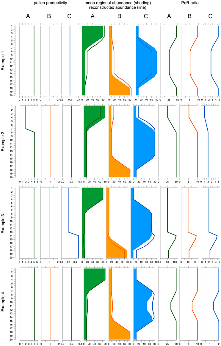
Figure 1. Behavior of the PAR over REVEALS (PoR) ratio when one PPE is wrong (example 1), under changing pollen productivity (example 2 and 3) and under changing total regional plant abundances (example 4). The model includes three taxa A, B, and C over 20 time steps (y-axis): Taxon A (green) is dominant in the top part, B (orange) in the lower part and C (blue) in the middle part of the record. Default pollen productivity is 5 for A, 1 for B and 0.2 for C. Line graphs to the left depict actual pollen productivity in each example. Graphs in the middle depict true abundances (shading) and abundances reconstructed with REVEALS (lines). Graphs to the right depict the PoR ratio. In example 1, the PPE of C used in the REVEALS reconstruction is set at 0.5 instead of 0.2. As a result, the cover of C is underestimated and consequently that of A and B overestimated. The PoR ratio is lower for all taxa where C is abundant. In example 2, pollen productivity of A is reduced from 5 to 2 in the upper 7 samples. REVEALS is still applied with a PPE of 5. Hence, the cover of A is underestimated and consequently that of B and C overestimated. The PoR ratio is reduced for all three taxa. In example 3, the pollen productivity of C is increased from 0.2 to 0.5 in the 7 lower samples, with opposite effects to example 2. In example 4, the sum of all abundances is reduced from 100 to 70% in samples 10-12. REVEALS does not reflect this change in total abundances. Hence the reconstructed cover of all three taxa is too high in the central part and PoR values are reduced correspondingly. Note that if the correct PPEs and total abundances are used, reconstructions fit true abundances and PoR ratios are always the same (samples 20-8 in example 2, 13-1 in example 3, and 20-15 plus 7-1 in example 3). As the K-factor is equal for all taxa the ratio between the PoR values equals the ratio between the PPEs.

A spreadsheet file containing raw data and calculations of all following examples is available as Supplementary Data.

The PoR Ratio With a Wrong PPE

The first experiment shows an error in one of the PPEs used in the reconstruction; this is the type of error ROPES is designed to remove. In the example, abundances are reconstructed with an incorrect PPE of 0.5 instead of the correct PPE of 0.2 for taxon C. With this one PPE set too high, REVEALS produces a too low cover for taxon C and consequently a too high cover for A and B. Because the PAR values remain unchanged, all PoR ratios are affected. For C, the ratio is higher than it should be because the REVEALS reconstructed cover is too low in all samples. The effect is high in the top and bottom sections—where C is rare—and lower in the middle section—where C is abundant. If C is rare, the wrong PPE introduces a small absolute but high relative error in the reconstruction: in the top and bottom section the true cover is 5%, whereas the REVEALS reconstructed cover is only 2%, i.e., 60% lower. If C is abundant, the wrong PPE introduces a large absolute but a smaller relative error: in the middle section, the true cover is 75% while the REVEALS reconstructed cover is 50%, i.e., only 33% lower. For A and B, the PoR ratios are too low because total REVEALS reconstructed abundance is 100% and if the reconstructed abundance of C is too low, that of the two other taxa is necessarily too high. The aberration in the PoR ratios of A and B is highest where C is abundant because the absolute error in reconstructed cover is highest here. So, the use of wrong PPEs introduces variations in the PoR ratios of all taxa and these variations always run parallel for all taxa.

Variations in Pollen Productivity P

In example 2 (Figure 1), pollen productivity of taxon A is lowered from 5 to 2 in the upper 7 samples, so that its PAR values are 2.5 times lower than before. REVEALS is still applied with a PPE of 5. Hence, in the upper 7 samples the actual pollen productivity of A is lower than the applied PPE, so that the reconstructed cover of A is too low and consequently that of B and C too high. Now we observe that the PoR ratio of all three taxa is lower in the upper 7 samples. For B and C the explanation is simple; the reconstructed abundance is higher while PARs remain unchanged. For A the explanation is less obvious as both PAR values and reconstructed abundances are lower. However, the strong decline in PAR values is much suppressed in pollen proportions, which always add up to 100%, so that the decline is underestimated in the reconstructed abundances.

In example 3, pollen productivity of taxon C is elevated from 0.2 to 0.5 in the lower 7 samples (13–20); REVEALS is still applied with the default PPE of 0.2. Hence, in sample 13–20 actual pollen productivity is higher than the applied PPE, so that the reconstructed abundance of C is too high and consequently that of A and B too low. We observe that the PoR ratio of all three taxa is higher in sample 13–20. Again, for A and B the ratio is elevated simply because their reconstructed abundance is lower while PARs remain unchanged. For C, the strong increase in PARs is suppressed in the pollen proportions, so that the increase is also underestimated in the reconstructed abundances. So, a temporarily lower pollen productivity of one taxon causes lower PoR ratios for all taxa and vice versa. These variations always run parallel for all taxa.

Variations in the Total Area A

The PoR ratio is expected to be constant only if the sum of all mean regional abundances (A in Equation 6) is constant. This sum may change for example when sea level rise reduces the area of pollen producing land or when humans create bareland. Furthermore, the sum of regional abundances only reflects taxa that are represented in the pollen record, i.e., it may change when plants that are not or poorly represented in the pollen record expand or decline, e.g. immature trees or potato. In our example 4, the total cover of the three taxa is 100% in the top and bottom section but only 70% in sample 10-12. The REVEALS reconstructed abundance necessarily sums up to 100% in all samples and does not reflect changes in total plant abundance in the middle section. PAR values do reflect the change and are lower, so that the PoR ratio of all taxa is lower as well. So, if the sum of regional abundances declines, the PoR ratio of all taxa will decline as well, and vice versa.

Variations in the Dispersal and Deposition Factor K

The PoR ratio will also be influenced by the processes of pollen dispersal and finally deposition in a lake as expressed by the K factor (cf. Equation 6). Whether and how atmospheric circulation has changed in the past, and how such changes may have altered pollen dispersal, is poorly understood. Pollen deposition in a large lake may change when lake size and morphometry change. ROPES is limitedly suited for records affected by such changes.

In addition to the above three modes of variation (in P, A, and K), error in the PAR values will introduce short-lived fluctuations in the PoR ratio around a mean value. Error in the PAR values is mainly related to dating uncertainties and error in exotic marker counts. In the following tests we will explore how error in the PAR values affects ROPES by adding noise to the PAR data in our tests.

Example Applications

Methods

Implementation of ROPES

We have implemented ROPES in the R environment for statistical computing (R Core Team, 2016). The core of ROPES is to minimize variation in the PoR ratio by adjusting initially random PPEs for each taxon. For optimization we use the “DEoptim” function (Ardia et al., 2011a,b, 2015; Mullen et al., 2011), an algorithm suited to find global optima. Before optimization, first the dispersal- and deposition factor K is calculated for each taxon. K is a distance-weighted representation of the amount of pollen arriving from beyond the basin radius. Mathematically, K is expressed as the pollen deposition of a taxon in a lake or peatland with a given diameter divided by deposition in a basin with zero diameter. K depends on the fall speed of a pollen taxon and on the dispersal model used for simulations. In ROPES, K is calculated with the “DispersalFaktorK” function from the DISQOVER package, which by default uses the state-of-the-art Lagrangian stochastic dispersal model (Theuerkauf et al., 2016).

Optimization starts with assigning a random PPE between 0.01 and 20 to each taxon. DEoptim then calls a target function, which in three steps calculates the single target value that is to be optimized. It first calculates vegetation composition for each pollen sample using the “REVEALSinR” function from the DISQOVER package, with the respective K factors and the initially random PPEs. It then calculates the PoR ratio for each taxon and sample by dividing PAR values by the reconstructed abundances. For each taxon, the PoR ratio is normalized through division by the average PoR ratio over all samples. Finally, the target function calculates and returns overall variance in the PoR ratios. Overall variance is expressed as the sum of variance over all taxa, calculated as standard deviation of the PoR ratio divided by the mean PoR ratio over all samples. The optimization algorithm iteratively optimizes PPEs to arrive at the lowest possible overall variance.

Synthetic Data

To test and illustrate the potentials of ROPES, we use synthetic datasets based on virtual landcover and associated pollen. For these synthetic datasets the true relationship between pollen and vegetation is known so that the performance of the ROPES reconstruction tool can be evaluated. We wanted to create realistic datasets that show similar pollen composition and changes as real pollen records. For that reason, time series of virtual landcover were not created randomly but constructed on the basis of real pollen datasets from three lakes in NE-Germany (Gadowsee GAD, Stinthorst STI and Tiefer See TSK). To that end, we translated these empiric pollen data into vegetation composition using the REVEALSinR function from the R package DISQOVER with standard settings for pollen dispersal and PPEs from the PPE.MV 2015 data set (PPEs derived from sites in NE Germany, Theuerkauf et al., 2016). For REVEALS modeling, only the 19 most common taxa were selected (Table 1). We adopted these reconstructions as the time series of virtual landcover.

TABLE 1

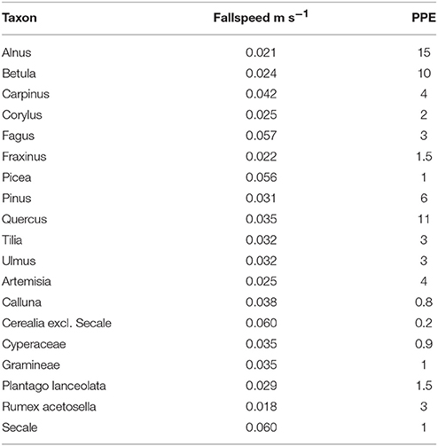
Table 1. PPEs and fall speed of pollen used to prepare synthetic pollen data sets.

In step two, these time series were used to derive synthetic pollen records. Pollen accumulation rates (PAR) were calculated by multiplying virtual abundance of each taxon by its respective (synthetic) PPE (Table 1), K factor and an arbitrary scaling factor of 100 so that the resulting values are of similar magnitude as empiric PARs. Based on these synthetic PAR data, pollen counts were calculated assuming a pollen sum of 1,000. These synthetic pollen counts deviate from the empiric counts they are based on, but do show similar trends and complexity. Both synthetic PARs and pollen counts were then used in the ROPES tests.

We created 3 synthetic data sets: GAD, STI, and TSK (Tables 1, 2). Experiments with these data sets focus on data complexity and error in pollen data. To explore the influence of sample size on ROPES, we use three versions of each data set with 60, 130, and 250 pollen samples, respectively. The original number of samples for the GAD record was 60, for STI 130 and for TSK 250. Additional versions of the three records were created by either deleting or adding samples in the original data sets. PAR values for new samples were calculated as the mean of the two adjoining samples. ROPES was thus tested on a total of 9 data sets (Table 2). To underline the hypothetical nature of our reconstructions, pollen and plant taxa are written in normal font throughout the manuscript.

TABLE 2

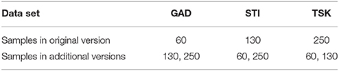
Table 2. Main parameters of the pollen data sets.

Error in Pollen Data

To mimic uncertainty in pollen data, noise was added in pollen counts and PARs. Noise in the counts is calculated by randomly drawing pollen samples with 1,000 pollen grains based on the composition of the synthetic pollen deposition. Samples were drawn with the R-function “rmultinom,” where probabilities “prob” equal pollen proportions in the synthetic data and sample “size” represents the pollen sum (= 1000). Noise in PARs is in addition related to uncertainty in the exotic marker counts and error in sample accumulation rates—both affect all taxa in a sample in a similar way. We thus added a random component to the PAR value of all taxa in a sample. This component is calculated as the actual PAR value times a random value drawn from a normal distribution, centered around 0, and divided by a fixed factor. For each data set we tested two variants, one with division factor 10 to mimic intermediate error and one with division factor 5 to mimic large error in PAR data. In this way, the noise is similar to noise observed in real pollen data sets, as illustrated by a comparison with data from the partly laminated Lake Tiefer See (Dräger et al., 2017, Figure 2). For this quick comparison, we calculated sample to sample variation in the pollen data sets as the absolute difference in PAR between two consecutive samples divided by the PAR of the first of those samples. It should be noted that this calculation actually conflates signal and noise and thus overestimates true noise.

FIGURE 2

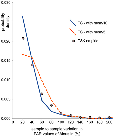
Figure 2. Comparison of sample-to-sample variation (as an indicator of noise) in empiric and synthetic PAR records. Sample-to-sample variation is calculated as the relative difference between two consecutive PAR values, here for Alnus. The values, plotted as probability density, show that noise in the empiric PAR record from Lake Tiefer See is somewhat larger than in the derived synthetic PAR record with intermediate error added (TSK with rnom/10) and somewhat smaller than in the derived PAR record with large error added (TSK with rnom/5).

Model Runs and Evaluation

We applied ROPES on the 9 synthetic data sets with 4 types of error in the pollen data, making a total of 36 experiments (Figure 3). For each experiment, 100 model runs were conducted with newly drawn random error added in each run. To guarantee that global optima are found, convergence parameters of DEoptim are set to high sensitivity: reltol to 0.00001 and steptol to 500 (see Ardia et al., 2015). To evaluate model performance we assess accuracy of the reconstructed plant cover as well as of the ROPES-based PPEs. To asses accuracy of reconstructed plant cover, first the absolute difference is calculated for each pair of the original (synthetic) and the reconstructed plant cover (i.e., 3 records times 19 taxa times 60, 130, and 250 pairs). To represent the proportion of the landscape for which the reconstruction is wrong for a given pollen sample, the difference is summed up over all taxa and divided by two. Division by 2 corrects for the fact that values are expressed as percentages and any error in the cover of one taxon is mirrored by an equally large opposite error in other taxa, resulting in a maximum possible absolute error of 200% (cf. Theuerkauf and Couwenberg, 2017). Finally, the mean error over all samples in a record is calculated to represent the inaccuracy of a given model run. To asses accuracy of the ROPES-based PPEs we compare the median PPE of the 100 model runs with the original PPEs of Table 1.

FIGURE 3

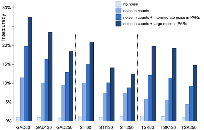
Figure 3. Inaccuracy of ROPES reconstructed landcover expressed as mean proportion of the landscape for which the reconstruction is wrong. Accuracy is assessed for 9 synthetic data sets representing 3 sites (GAD, STI, and TSK) each with 3 sizes (60, 130, and 250 samples). Four different types of error are applied (no error, error in pollen counts, error in counts plus intermediate noise in PAR values, and error in counts plus large noise in PAR values).

Real World Example

As a first real world example, we apply ROPES with original pollen data from Lake Tiefer See (cf. Dräger et al., 2017). Also here analysis is restricted to the 19 most common taxa. The range of potential PPEs is again set to 0.01–20. ROPES is applied with the same settings as before, no additional error was added to the pollen data.

Results and Interpretation

Reconstructed Landcover

With no error added in pollen data, ROPES produces near-perfect results in all 9 synthetic data sets. Error in the reconstructed landcover amounts to around 1%, i.e., the reconstruction is correct for 99% of the synthetic study area. With ideal data ROPES is evidently well able to reconstruct past landcover with short as well as long pollen records. With noise added to the pollen counts, error in the reconstructed landcover amounts to ~5% in the TSK data sets and to ~10% in the GAD and STI data sets. ROPES performs somewhat better with the longer records, but overall the number of samples has limited effect on the results if noise is added to the counts only.

Adding noise also in the PAR data further increases the error in the reconstruction. With intermediate noise, error in the reconstructed landcover increases to 9–19%. The error is smallest in the long STI and TSK records (STI130, STI250, TSK130, and TSK250), intermediate in STI60 and TSK60, and highest in GAD130 and GAD60. With large noise in the PAR data, error ranges from 12 to 29%. Again, performance is best with the long STI and TSK records whereas the largest error occurs with the short records GAD60 and GAD130. Still, also with large noise added, ROPES in most cases correctly reconstructs landcover for more than 75% of the landscape.

Pollen Productivities

Besides landcover, ROPES also reconstructs PPEs for the taxa involved. With no noise in the pollen data, the median PPE over 100 model runs is mostly close to the true PPE in the experiments with GAD and TSK records. Experiments with the STI record for some taxa produce too low (Plantago lanceolata, Secale) or too high PPEs (Artemisia, Cerealia, Figure 4). With noise in the pollen data, the median PPEs deviate more from true pollen productivity. The error remains lowest with the TSK records, where—with full noise added to the data—for most taxa (e.g., Carpinus, Fagus, Calluna, and Secale) the reconstructed PPEs deviate little (<20%) from true pollen productivity. The largest mismatch with TSK is for Fraxinus, for which PPEs with full noise are ~30% too low. Error tends to be higher with the GAD records, where with GAD60 and full noise the overall highest mismatch occurs for the PPE of Tilia (20 instead of 3). For Artemisia, Rumex and Ulmus, PPEs derived from noisy or short GAD records are less than half the original pollen productivity. In all other cases, PPEs are within 50–200% of the original value. With noise added to the data, STI produces PPEs that are outside this error range for Carpinus, Fagus Artemisia, Plantago lanceolata, Rumex, and Secale.

FIGURE 4

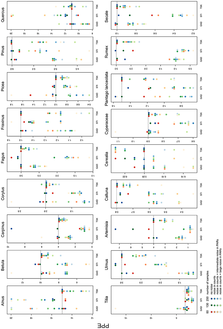
Figure 4. Median of PPEs produced in each of the 36 experiments. The colors represent the sample size, shades represent the noise added in the pollen data. Dotted lines show original pollen productivity of each taxon. Note the scaling of the y-axes. For full results see Supplementary Material.

With full noise in the data, a number of single ROPES runs for some taxa approximate PPEs at the pre-defined upper margin of 20 (see Supplementary Data). This mainly applies to Alnus, Betula and Quercus, i.e., the taxa with highest pollen productivity, and only rarely for other taxa.

We have outlined before that ROPES requires sufficient variation and number of samples in the pollen record. This raises the question whether taxa with little variation (including rare taxa) hamper the reconstruction of taxa with sufficient variation. To answer this question we explore how error in the PPE of a taxon relates to its range in pollen percentage values and number of samples (Figure 5). With no noise in the pollen data, error in the PPEs is mostly small (<10%), except for some taxa from the STI record which show very little variation along the record. With noise in pollen counts error in the PPEs is clearly higher, increasing slightly with intermediate and large noise added in the PAR data. As before, high errors (>40%) are restricted to taxa with little variation through the pollen record, i.e. taxa that are either always rare or occur with very stable values. Errors >40% rarely occur when total range in pollen values times number of samples in a record is larger than 2,000. We conclude that short, noisy data sets are still suited to produce suitable PPEs for taxa that cover a large range in pollen percentage data. As a tentative rule of thumb, PPEs tend to be reliable when the range in pollen values multiplied by the number of samples is larger than 2,000.

FIGURE 5

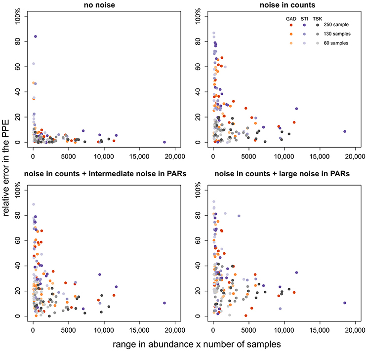
Figure 5. Relative PPE error (y-axis) plotted over the range of values of the respective taxon multiplied by the number of samples (x-axis). PPE error is calculated as the absolute difference between the median from 100 model runs and true pollen productivity divided by true pollen productivity (×100%). The colors denote the pollen record, shade its size.

Application of ROPES with pollen data from Lake Tiefer See produced a set of palaeo-PPEs, i.e., PPEs based on a long Holocene pollen record, which we compare with PPEs based on surface studies (Figure 6). Both data sets show high PPEs for most tree taxa, in particular Alnus, Betula, Corylus, and Quercus, and low PPEs for most herb taxa. Despite the overall similarities, we also observe some differences. For Alnus, Betula, Corylus, Artemisia and Rumex acetosella, PPEs produced with ROPES are clearly lower than those from the surface sample record, for Cerealia excl. Secale and Gramineae, PPEs produced with ROPES are clearly higher.

FIGURE 6

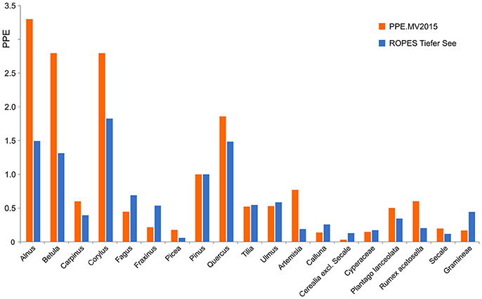
Figure 6. PPEs produced with ROPES from the Lake Tiefer See record (TSK, 250 samples) compared with the PPE.MV 2015 set of PPEs from Theuerkauf et al. (2016).

Advantages and Limitations

Our tests have shown that ROPES is indeed able to reconstruct landcover and PPEs. The performance differs among the 36 experiments, mainly in response to sample size, variance along the record and noise in the pollen data. ROPES performs near perfect in the experiments with no noise in the pollen data, which demonstrates the validity of the approach. Particularly noise in the PAR data introduces error in the reconstructions of landcover and PPEs. Error is larger the shorter and less diverse the record. Increasing sample size in almost all cases reduces error in the reconstruction both in terms of landcover and PPEs. It is likely that performance will further improve with records longer than those tested here. Still, also short records are suited to estimate the pollen productivity at least for taxa with a wide range of percentage values along the record.

Variation along the pollen record is essential for the functioning of ROPES: with no variation in the pollen record there is no variation in the PoR ratio with any set of PPEs so that ROPES cannot approach an optimal solution. In turn, the larger the variation in the pollen record, the better ROPES performs. We find that this relationship applies to each separate taxon in a record, i.e., ROPES performs better for the more variable taxa. The STI record is dominated by Pinus in all samples, leaving low proportional abundance and little variation for the other taxa. Correspondingly, ROPES performs well in reconstructing cover and pollen productivity of Pinus but not of the rare taxa. The TSK record is more diverse; most taxa are abundant at least in some sections of the record. ROPES therefore performs well in reconstructing PPEs and cover of most taxa. Still, the overall landcover reconstruction for STI is as good as or even better than that for TSK because of the good result for Pinus as the dominant taxon. So, if the aim is to produce pollen productivity of as many taxa as possible, diverse data sets with large variations in all taxa are needed. If the focus is on the landcover reconstructions itself, less diverse data sets dominated by one or few taxa are still suitable.

As a tentative rule of thumb we suggest that PPEs can be reconstructed for taxa for which the amplitude in the pollen percentage data multiplied by the number of samples is larger than 2,000. For an in depth evaluation of a data set we suggest to apply sensitivity tests similar to those presented here. Such an evaluation, in which synthetic data are tested that are based on an actual pollen record, can show the specific capabilities and limits of a particular data set.

Future Applications-Potentials and Limits

ROPES does not depend on pre-defined PPEs—it thus has the potential to expand quantitative landcover reconstruction into areas for which such calibration is not yet available or not feasible. For these areas, ROPES would then not only provide initial landcover reconstructions but also PPEs. Each successful ROPES application may thus trigger follow-up reconstructions with existing approaches, such as REVEALS, that employ percentage pollen data and PPEs.

Although often disregarded, application of quantitative reconstructions is so far limited to areas and periods for which the available correction factors are suited. PPEs for example are derived and only applicable in a specific space-time. Consequently, the common use of mean PPEs amalgamated across large areas that show considerable differences in land use, soil types, slope and climate (Broström et al., 2008; Mazier et al., 2012) implies additional error in the reconstruction. Moreover, PPEs derived from modern pollen-landcover relationships are applied to ancient situations, although pollen productivity has changed in the past (Waller et al., 2012; Feeser and Dörfler, 2014; Theuerkauf et al., 2015). ROPES may help reduce these limitations and provide targeted reconstructions for non-analog situations, e.g., of Lateglacial vegetation of Europe. In this way, ROPES may contribute to a better understanding of vegetation dynamics in times of climate change. It probably can help explore whether and how pollen productivity of plant taxa responds to changes in climate, species composition or land management. In ROPES, periods of changing pollen productivity are expressed as changes in the PoR ratio. To fully explore the actual changes in pollen productivity, ROPES has to be applied separately on those sections of the record that were identified as distinct in the first round. The limitation to this approach is that each section is required to retain sufficient variation, i.e., it has to have a minimum length. Approaches to optimize between section length and accuracy of the resulting PPEs still need to be developed. Changes in pollen productivity will likely be observable over millennial, rather than centennial time scales.

A problem so far neglected in quantitative vegetation reconstruction is the presence of non-pollen producing areas. Quantitative approaches such as REVEALS assume that the taxa involved cover a fixed proportion of the surrounding area (commonly assumed to be 100%). In reality, some proportion of this area may be barren, open water, or covered by taxa that are virtually not represented in the pollen record, e.g., crops such as potato or trees such as Acer. ROPES has the potential to detect such effects and actually reconstruct non-pollen producing areas. The tests presented in this paper do not address the effect, but first attempts at reconstructing non-pollen producing areas have shown promising results. Approaches to proper weighing between correcting for errors in pollen productivity and total land cover are currently under development.

Our tests show that ROPES requires pollen records with limited noise in the PAR data. We already identified a number of suitable records, and are optimistic that many more exist. With the option to use PAR data in ROPES, we encourage analysts to estimate PARs as precisely as possible. To arrive at accurate pollen concentrations, sample volumes should be well defined and a sufficient number of exotic marker grains should be added to each sample. As the exotic marker grains serve as the basis for all further calculations, counts should amount to at least several hundred exotic grains to reduce statistical noise in PAR values. To guarantee that such an amount of exotic markers is counted it may be necessary to add multiple marker tablets to each sample. Care should be taken to still count at least as many “pollensum”-pollen, so as not to burden the REVEALS reconstructions with too much noise.

The next step, from pollen concentrations to PARs, requires sediment accumulation rates. Annually laminated sediments allow for exact dating and therefore such records appear most suited for ROPES. In non-laminated records accumulation rates can only be approximated from age-depth models. Giesecke and Fontana (2008) have shown that PARs with little noise can indeed be estimated in non-laminated lakes. We assume that also large peatlands may be suited to produce robust PAR values. In any case, the pollen dispersal model underlying ROPES assumes atmospheric pollen deposition exclusively. As implemented, ROPES is therefore thus far only applicable to closed lake basins and peat deposits.

The first application of ROPES on the empiric pollen record from Lake Tiefer See shows an overall good match between surface sample PPEs and PPEs produced with ROPES, which supports the general validity of the ROPES approach. There may be various reasons for the observed differences in the PPEs.

For example, the ROPES PPE of Corylus is lower than its surface sample PPE. The surface sample PPE is likely too high because Corylus is underrepresented in the forest inventories underlying surface sample PPEs (Theuerkauf et al., 2013). Similarly, the cover of herbs such as Artemisia and Rumex has likely been underestimated in surface sample studies, again resulting in too high PPEs. A higher palaeo-PPE for Cerealia excl. Secale could be explained by a focus on different species or cultivars within this group in the past, which were better reflected in the pollen record. The surface sample PPE of grasses is likely too low because pollen production in grasses is suppressed under present-day land management (Theuerkauf et al., 2015). A comprehensive discussion on PPEs produced with ROPES requires a more in depth analysis of further data sets.

Concluding Remarks

Existing methods of quantitative vegetation reconstruction correct for the productivity bias in pollen data with correction factors such as PPEs that are calibrated in the present day cultural landscape. This approach is not only laborious and far from simple, it also introduces unknown error in the reconstruction of past vegetation because PPEs calibrated in the modern cultural landscape may not be representative for the past. ROPES corrects for the productivity bias using pollen data only and without calibration. We see three major benefits for future landcover reconstructions.

First, ROPES may provide a shortcut to landcover reconstructions in new study regions if at least one site with suitable PAR and percentage pollen data is available. ROPES can deliver a landcover reconstruction for that site, and the PPEs needed to produce landcover reconstructions from further records in the region that are not suited for ROPES using other quantitative methods.

Secondly, ROPES can help improve and sharpen landcover reconstructions. The ability to estimate PPEs from single sites may allow exploring spatial patterns in pollen productivity within and between regions, e.g., in relation to variations in climate, soils and species composition. A better understanding of these interactions will enable more detailed reconstructions.

Thirdly, ROPES allows for landcover reconstructions for periods with non-analog climate and landcover, like the Lateglacial. Landcover reconstructions have been problematic for such periods because PPEs calibrated in the modern world are obviously unsuited.

Overall, our first tests suggest that ROPES will help shift away from PPEs as static parameters toward PPEs that are reconstructed from the (palaeo-)pollen record. ROPES thus adds past pollen productivity as an observable variable to palaeo-ecology. The approach has the potential to significantly improve landcover reconstructions and broaden their application, while adding additional insights.

Author Contributions

MT und JC jointly developed the idea of ROPES and the theory behind it. Both created the tests and wrote the manuscript. MT analyzed pollen of the original GAD, STI, and TSK records and implemented ROPES in R for the DISQOVER package.

Funding

This study is a contribution to the Virtual Institute of Integrated Climate and Landscape Evolution Analysis—ICLEA—of the Helmholtz Association (VH-VI-415) and to BaltRap: The Baltic Sea and its southern Lowlands: proxy—environment interactions in times of Rapid change (SAW-2017-IOW2). The work of JC was funded by the European Social Fund (ESF) and the Ministry of Education, Science and Culture of Mecklenburg-Western Pomerania (project WETSCAPES, ESF/14-BM-A55-0030/16).

Conflict of Interest Statement

The authors declare that the research was conducted in the absence of any commercial or financial relationships that could be construed as a potential conflict of interest.

Acknowledgments

We thank Almut Mrotzek and Marie-José Gaillard for valuable comments on the manuscript. We gratefully acknowledge the friendly and constructive remarks of two reviewers.

Supplementary Material

The Supplementary Material for this article can be found online at: https://www.frontiersin.org/articles/10.3389/feart.2018.00014/full#supplementary-material

Table S1. Principle of the ROPES approach illustrated using a record with just two samples and two taxa A and B. For both samples, PAR values and pollen counts (shown as percentage values) are known (left part of the table). REVEALS is applied on the pollen counts with the PPE of taxon A set to 1,2,3, …,10. B is the reference taxon with a PPE of 1. The right part of the table shows relative abundance reconstructed in each of these 10 REVEALS applications and the PoR ratio, i.e., the ratio of PAR value over REVEALS reconstructed cover. Only if the PPE of A = 5, the change in the reconstructed abundance of A and B (expressed as the value of sample 1 divided by sample 2 × 100%) is the same as the change in PAR values. As a result the PoR ratio is the same for both samples.

The synthetic and empiric pollen data used in the ROPES example applications are available for download from https://doi.pangaea.de/10.1594/PANGAEA.886900.

The R-code for ROPES is available from https://github.com/MartinTheuerkauf/ROPES.

References

Ardia, D., Arango, J. O., and Gomez, N. G. (2011a). Jump-diffusion calibration using differential evolution. Wilmott Magazine 55, 76–79. doi: 10.1002/wilm.10034

CrossRef Full Text | Google Scholar

Ardia, D., Boudt, K., Carl, P., Mullen, K. M., and Peterson, B. G. (2011b). Differential evolution with DEoptim: an application to non-convex portfolio optimization. R J. 3, 27–34. Available online at: https://journal.r-project.org/archive/2011-1/RJournal_2011-1_Ardia et al.pdf

Google Scholar

Ardia, D., Mullen, K. M., Peterson, B., and G Ulrich, J. (2015). DEoptim: differential evolution in R. Available online at: https://cran.r-project.org/web/packages/DEoptim/index.html

Broström, A., Nielsen, A. B., Gaillard, M.-J., Hjelle, K. L., Mazier, F., Binney, H. A., et al. (2008). Pollen productivity estimates of key European plant taxa for quantitative reconstruction of past vegetation: a review. Veg. Hist. Archaeobot. 17, 461–478. doi: 10.1007/s00334-008-0148-8

CrossRef Full Text | Google Scholar

Davis, M. B. (1967). Pollen accumulation rates at Rogers Lake, Connecticut, during late-and postglacial time. Rev. Palaeobot. Palynol. 2, 219–230. doi: 10.1016/0034-6667(67)90150-9

CrossRef Full Text | Google Scholar

Dräger, N., Theuerkauf, M., Szeroczynska, K., Wulf, S., Tjallingii, R., Plessen, B., et al. (2017). Varve microfacies and varve preservation record of climate change and human impact for the last 6000 years at Lake Tiefer See (NE Germany). Holocene 27, 1–15. doi: 10.1177/0959683616660173

CrossRef Full Text

Feeser, I., and Dörfler, W. (2014). The glade effect: vegetation openness and structure and their influences on arboreal pollen production and the reconstruction of anthropogenic forest opening. Anthropocene 8, 92–100 doi: 10.1016/j.ancene.2015.02.002

CrossRef Full Text | Google Scholar

Giesecke, T., and Fontana, S. L. (2008). Revisiting pollen accumulation rates from Swedish lake sediments. Holocene 18, 293–305. doi: 10.1177/0959683607086767

CrossRef Full Text | Google Scholar

Hicks, S. (1999). The relationship between climate and annual pollen deposition at northern tree-lines. Chemos. Glob. Change Sci. 1, 403–416. doi: 10.1016/S1465-9972(99)00043-4

CrossRef Full Text | Google Scholar

Hicks, S. (2001). The use of annual arboreal pollen deposition values for delimiting tree-lines in the landscape and exploring models of pollen dispersal. Rev. Palaeobot. Palynol. 117, 1–29. doi: 10.1016/S0034-6667(01)00074-4

CrossRef Full Text | Google Scholar

Matthias, I., Nielsen, A. B., and Giesecke, T. (2012). Evaluating the effect of flowering age and forest structure on pollen productivity estimates. Veg. Hist. Archaeobot. 21, 471–484. doi: 10.1007/s00334-012-0373-z

CrossRef Full Text | Google Scholar

Mazier, F., Gaillard, M. J., Kuneš, P., Sugita, S., Trondman, A. K., and Broström, A. (2012). Testing the effect of site selection and parameter setting on REVEALS-model estimates of plant abundance using the Czech quaternary palynological database. Rev. Palaeobot. Palynol. 187, 38–49. doi: 10.1016/j.revpalbo.2012.07.017

CrossRef Full Text | Google Scholar

Mullen, K., Ardia, D., Gil, D., Windover, D., and Cline, J. (2011). DEoptim: an R package for global optimization by differential evolution. J. Stat. Softw. 40, 1–26. doi: 10.18637/jss.v040.i06

CrossRef Full Text | Google Scholar

Prentice, I. C., and Webb, T. (1986). Pollen percentages, tree abundances and the Fagerlind effect. J. quarter. Sci. 1, 35–43 doi: 10.1002/jqs.3390010105

CrossRef Full Text | Google Scholar

Prieto-Baena, J. C., Hidalgo, P. J., Domínguez, E., and Galán, C. (2003). Pollen production in the Poaceae family. Grana 42, 153–159. doi: 10.1080/00173130310011810

CrossRef Full Text | Google Scholar

R Core Team. (2016). R: A Language and Environment for Statistical Computing. Vienna: R Foundation for Statistical Computing.

Seppä, H., and Hicks, S. (2006). Integration of modern and past pollen accumulation rate (PAR) records across the arctic tree-line: a method for more precise vegetation reconstructions. Quarter. Sci. Rev. 25, 1501–1516. doi: 10.1016/j.quascirev.2005.12.002

CrossRef Full Text | Google Scholar

Sugita, S. (2007). Theory of quantitative reconstruction of vegetation I: pollen from large sites REVEALS regional vegetation composition. Holocene 17, 229–241. doi: 10.1177/0959683607075837

CrossRef Full Text | Google Scholar

Theuerkauf, M., and Couwenberg, J. (2017). The extended downscaling approach: a new R-tool for pollen-based reconstruction of vegetation patterns. Holocene 27, 1252–1258. doi: 10.1177/0959683616683256

CrossRef Full Text | Google Scholar

Theuerkauf, M., Couwenberg, J., Kuparinen, A., and Liebscher, V. (2016). A matter of dispersal: REVEALSinR introduces state-of-the-art dispersal models to quantitative vegetation reconstruction. Veget. Hist. Archaeobot. 25, 541–553. doi: 10.1007/s00334-016-0572-0

CrossRef Full Text | Google Scholar

Theuerkauf, M., Dräger, N., Kienel, U., Kuparinen, A., and Brauer, A. (2015). Effects of changes in land management practices on pollen productivity of open vegetation during the last century derived from varved lake sediments. Holocene 25, 733–744. doi: 10.1177/0959683614567881

CrossRef Full Text | Google Scholar

Theuerkauf, M., and Joosten, H. (2012). Younger Dryas cold stage vegetation patterns of central Europe - climate, soil and relief controls. Boreas 41, 391–407. doi: 10.1111/j.1502-3885.2011.00240.x

CrossRef Full Text | Google Scholar

Theuerkauf, M., Kuparinen, A., and Joosten, H. (2013). Pollen productivity estimates strongly depend on assumed pollen dispersal. Holocene 23, 14–24. doi: 10.1177/0959683612450194

CrossRef Full Text | Google Scholar

von Post, L. (1918). Skogsträdpollen i sydsvenska torvmosselagerföljder. Forhandlinger ved de 16. Skandinaviske Naturforsheresmøte 1916, 433–465.

Waller, M., Grant, M. J., and Bunting, M. J. (2012). Modern pollen studies from coppiced woodlands and their implications for the detection of woodland management in Holocene pollen records. Rev. Palaeobot. Palynol. 187, 11–28. doi: 10.1016/j.revpalbo.2012.08.008

CrossRef Full Text | Google Scholar