 Robert L. Wolpert
 Elaine T. Spiller
 Eliza S. Calder
- 1Department of Statistical Science, Duke University, Durham, NC, United States
- 2Department of Mathematics, Statistics, and Computer Science, Marquette University, Milwaukee, WI, United States
- 3School of Geosciences, University of Edinburgh, Edinburgh, United Kingdom
To mitigate volcanic hazards from pyroclastic density currents, volcanologists generate hazard maps that provide long-term forecasts of areas of potential impact. Several recent efforts in the field develop new statistical methods for application of flow models to generate fully probabilistic hazard maps that both account for, and quantify, uncertainty. However, a limitation to the use of most statistical hazard models, and a key source of uncertainty within them, is the time-averaged nature of the datasets by which the volcanic activity is statistically characterized. Where the level, or directionality, of volcanic activity frequently changes, e.g., during protracted eruptive episodes, or at volcanoes that are classified as persistently active, it is not appropriate to make short term forecasts based on longer time-averaged metrics of the activity. Thus, here we build, fit and explore dynamic statistical models for the generation of pyroclastic density currents from Soufrière Hills Volcano (SHV) on Montserrat including their respective collapse direction and flow volumes based on 1996–2008 flow datasets. The development of this approach allows for short-term behavioral changes to be taken into account in probabilistic volcanic hazard assessments. We show that collapses from the SHV lava dome follow a clear pattern, and that a series of smaller flows in a given direction often culminate in a larger collapse and thereafter directionality of the flows changes. Such models enable short term forecasting (weeks to months) that can reflect evolving conditions such as dome and crater morphology changes and non-stationary eruptive behavior such as extrusion rate variations. For example, the probability of inundation of the Belham Valley in the first 180 days of a forecast period is about twice as high for lava domes facing Northwest toward that valley as it is for domes pointing East toward the Tar River Valley. As rich multi-parametric volcano monitoring datasets become increasingly available, eruption forecasting is becoming an increasingly viable and important research field. We demonstrate an approach to utilize such data in order to appropriately tune probabilistic hazard assessments for pyroclastic flows. Our broader objective with development of this method is to help advance time-dependent volcanic hazard assessment, by bridging the gap between eruption forecasting based on monitoring time series data and development of cutting edge probabilistic volcanic hazard maps.
1. Introduction
The Soufrière Hills Volcano (SHV), Montserrat, has been extensively studied since it erupted on 18 July, 1995 for the first time in centuries.
The multi-parametric datasets coupled with detailed observations of the surface activity for the main eruptive period facilitates exploration of forecasting models. Thus, SHV provides an ideal setting to build and explore next-generation models for short-term (weeks to months) pyroclastic density current forecasting where eruptive precursors and current conditions such as dome growth and orientation may be brought to bear (see Section 3.1). Here we propose models for the frequency, volume, and initial directions of pyroclastic density currents (PDCs) at SHV, with the end goal of improving forecasts for these sometimes devastating events. Most efforts at modeling for PDC forecasts either focus on retrospective forecasting (e.g., Sulpizio et al., 2010; Charbonnier and Gertisser, 2012) or long-term forecasting (e.g., Bayarri et al., 2009, 2015; Connor et al., 2012; Sandri et al., 2014; Neri et al., 2015), based on the stationary assumption that behavior remains constant over time. Recently, non-stationary models have been developed for long-term PDC forecasting (Bevilacqua et al., 2017) and for very long-term hazard evolution modeling (Jaquet et al., 2017). Non-stationary models have also been developed for, and applied to, modeling the state of volcanic systems (onset, active, repose, etc.) (e.g., Carta et al., 1981; Bebbington, 2007, 2010, 2012) and for forecasting volcanic events ≥VE1 (Bebbington, 2012). Here we present the first approach to short-term probability-based PDC forecasting based on dynamic statistical models.
Earlier, Bayarri et al. (2009) modeled the times of PDC events as a stationary stochastic process, with distributions for their volumes and initial directions that did not change over time. While our results suggest that this is adequate for long-term forecasts and hazard assessment (but see Bebbington, 2010; Bevilacqua et al., 2017; Jaquet et al., 2017 for a contrasting view), we show that the frequency and directional distribution vary markedly over shorter time intervals. Both Aspinall et al. (2003) and Woo (2018) have also highlighted the need for short-term, dynamic forecasting that can take into account monitoring and precursor information. Although much work toward this end focuses on combining probabilities of individual processes using Bayesian Belief Networks or Bayesian Event Trees (e.g., Marzocchi et al., 2008; Sandri et al., 2009; Hinks et al., 2014; Woo and Aspinall, 2014), this work does not focus on probabilistically modeling the individual components. Here we build dynamic statistical models in which PDC frequency alternates between high-activity and low-activity states, and in which the directional distribution can change following dome-collapse events.
The dates, valleys affected, and estimated volumes of 845 PDCs of volume ≥0.15·106m3 (i.e., 0.15 million cubic meters) recorded at the Montserrat Volcano Observatory (MVO) through July 2008 are reported in Ogburn et al. (2012), one of the most complete PDC dataset ever assembled. PDCs and rockfalls with volumes <0.15·106m3 are not recorded here. All of the modeling and data analysis in this work is based on that dataset, and by “PDC event” we will mean a PDC at SHV of volume at least 0.15·106m3.
Figures 1A,B show the drainage and valley structure surrounding SHV. Figure 1C shows the volumes (on log scale, as radius, with a small amount of jitter to reveal multiplicity) and initial angles (as azimuth counter-clockwise from due East) of all recorded PDCs. Only PDCs' valleys are known, so interval-censored PDC angles {ϕj} are represented as arcs Φj.
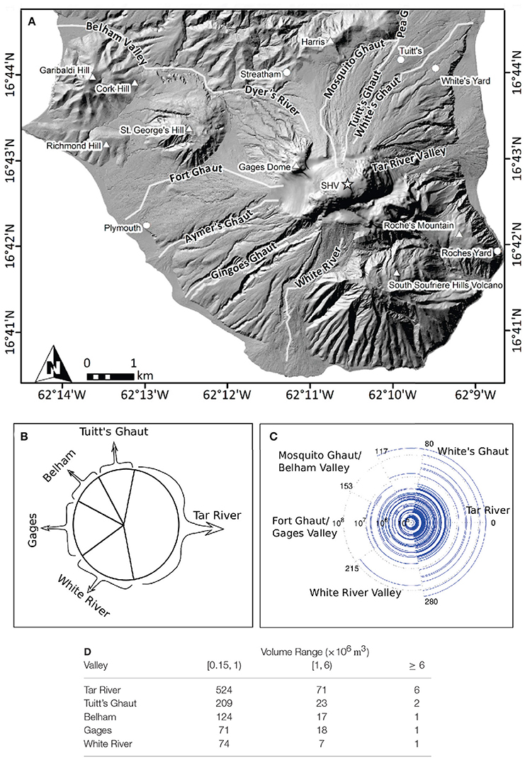
Figure 1. (A) Topographic map of southern Montserrat, showing SHV and valley contours. (B) Cartoon drawing illustrating major drainages (valley groups). (C) Empirical plot of PDC volumes Vj (as radius, on log scale) and initial directions ϕj (as angles counter-clockwise from due East, in degrees). (D) Tabulated counts of PDCs inundating the five major drainages, for each of three PDC volume ranges.
While there is some suggestion of heavier flow activity to the east, the evidence against independent uniform distributions is not strong. Further, the evidence against independence between uniformly distributed initiation angles {ϕj} and Pareto-distributed volumes {Vj} for significant flows is not strong (for flows exceeding 106m3, a chi-squared test of independence for categorized data with three levels of volume and five groups of valleys gave a value of χ2 = 13.3 on 8 degrees of freedom, for a p-value of 0.10 showing little evidence against independence).
While this stationary model may be reasonable for long-term forecasts (several years or more), there is evidence that it is not appropriate for short-term forecasts. The PDC frequency appears to vary over time, with alternating high-frequency and low-frequency periods; the angular distribution of initial flow angles appears non-uniform over short periods; and its distribution too may change over time.
Figure 2 shows directional tendencies for the periods between major PDCs (those whose volumes exceed 6·106m3), along with a red arc representing the valley inundated by the last major PDC of that period or epoch. Note the strong directional concentration within most of these periods, and the abrupt changes that often occur at the times of major PDCs at the end of each epoch. A Generalized Likelihood Ratio Test confirms that the angular distributions differ across epochs; see section (2.2.3) for details.
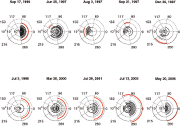
Figure 2. Volumes {Vj} and directions of flows {ϕj} during epochs (Te, Te+1] between major PDCs (those with volume V > 6·106m3). Thin black arcs indicate angular extent of direction of collapse of PDCs in this epoch; radii indicate volumes on logarithmic scale; thick red arcs show valley(s) of major flows at times {Te+1} (labeled above each subplot) ending each epoch.
Figure 3 presents the cumulative number of PDCs for the study period, just over 12 years following 1st January 1996. The slope of the line in this figure, measured in PDC events per year, is one measure of volcanic activity level. Evidently it is not constant over the decade shown and it is recognized that these changes relate, to first order, to the actual growth and pause periods of volcanic activity (Wadge et al., 2010).
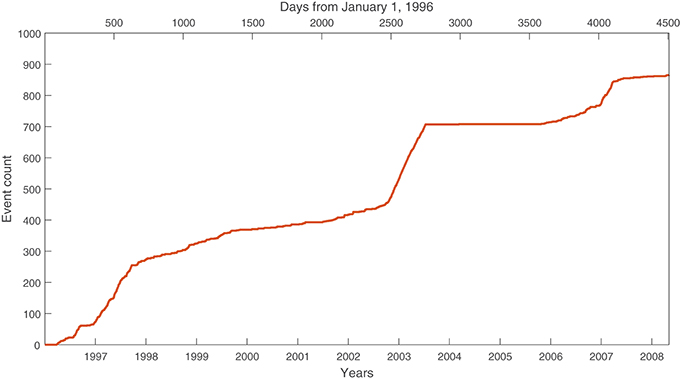
Figure 3. Cumulative count of PDC events, illustrating that PDC frequency varies over time. Note slope of curve is sometimes steep (in high-activity periods) and sometimes shallow (in low-activity periods or dome growth pauses).
Here we propose and support a new model for PDC generation whose frequency and whose initiation angle distributions are random stochastic processes. The PDC frequency jumps on occasion back and forth between two levels, one low and one high. The angular distribution is weighted toward some central direction toward which the lava dome grows; this direction will change to some randomly-chosen new direction following the generation of a major PDC and dome collapse event.
We employ the Objective Bayesian inferential paradigm (Berger et al., 2009) in order to reflect in our volcanic forecasts, both uncertainty about estimates of model parameters, as well as that arising from the natural uncertainty and variability of volcanic systems. In that paradigm, uncertainty about the model parameters of interest (e.g., slopes of cumulative PDC counts), here represented by a vector θ, is represented in the form of a posterior probability density function π(θ ∣ data), proportional (by “Bayes' Rule”) to the product of the likelihood function, f(data ∣ θ), and a prior density function π(θ) chosen to represent initial ignorance. We present and justify our choices of probability models (and hence the likelihood functions) and prior distributions, and then use Markov chain Monte Carlo (MCMC) numerical methods to generate both parameter estimates (with attendant measures of uncertainty) and model forecasts (also with uncertainty quantified), from their posterior distributions (Rosenthal, 2011).
With this model the conditional distribution of the time to the next PDC, and its magnitude and initial direction, may depend on known features of the data set, such as the directions and times of recent PDCs. In section (3.1) we illustrate how this can be used to improve short-term forecasts. It is worth noting that we do not model the (difficult to observe) magma ascent directly. That said, the timing of events (which we do model) and magma ascent share similar non-stationary patterns (Wadge et al., 2010), but only the event timing is readily observable here.
We present the model in two parts: first in section (2.1) we describe the model for the frequency of pyroclastic density currents, then in section (2.2) we describe the model for the volume and initial directions of those flows. In section (3.1) we illustrate and validate how this model can support short-term forecasting, by making model forecasts for a 3-year period following a specified date (we chose 1st January 2006), based only on data prior to that date, and comparing model forecasts to actual observations. Finally, in section (4) we present our conclusions and some directions for future development. Computational details and lists of hyperparameter values, probability distributions, mathematical notation, likelihood and posterior distributions are collected in an Appendix.
2. Methods
2.1. A Dynamic Model for Eruptive Activity
In this section we construct a model for the times of PDC events sufficiently large to be recorded at SHV, i.e., of volume 0.15·106m3 or more.
2.1.1. Modeling Variable PDC Frequency
Figure 3 illustrated that the volcanic frequency at Soufrière Hills does not appear to be uniform over time on a decade-long scale. To accommodate this we model the times {τj} of PDC events as an inhomogeneous Poisson point process with rate λ(t) that may vary with time. Thus, the numbers of events in disjoint time intervals (ai, bi] will have independent Poisson distributions with means given by
for an uncertain time-varying PDC frequency λ(t), measured in events/yr. The simplest choice for a function λ(t) that appears consistent with the data would be a two-state model in which λ(t) takes only two possible values 0 < λlo < λhi < ∞, switching from the low rate to the high rate and back at transition times {sm, tm} respectively, or
for 0 < s1 < t1 < s2 < …, beginning in the “low” state. Also introduce t0: = 0 to simplify formulas below (here the notation “a: = b” means that a is defined to be b). A simulation of such a function appears in Figure 4, with an observation period of [0, T] and a subsequent forecast period of (T, T′] with T = 10 year and T′ = 15 year. Note that the values of the rates λlo and λhi in the upper panel correspond to values of the slopes of the cumulative event counts in the lower panel.
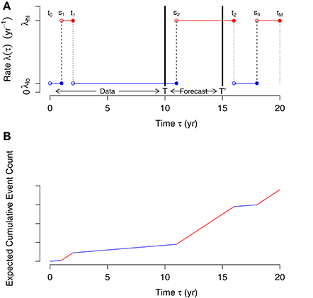
Figure 4. Simulated rate function λ(τ) of PDCs in top panel (A) and, in bottom panel (B), expected cumulative event count , plotted against time τ since eruption onset. Observation period [0, T] and forecast period (T, T′] are indicated, with T = 10 year and T′ = 15 year. Compare to observed cumulative event counts in Figure 3.
The likelihood function for the parameters and transition time vectors from such a realization will depend on the data vector of observed PDC event times in a specified observation period [0, T] only through two features of the data: the counts Nhi and Nlo of events that occur in periods of high and low activity, respectively, and the total amounts of time Thi and Tlo spent in those periods. These can be evaluated from the observed event times {τj} and modeled transition times {sm, tm} as follows:
Here the notation “(s, t]” denotes the interval of all those times τ for which s < τ ≤ t, with the inclusion of the right end-point indicated by a square bracket and the exclusion of the left end-point indicated by a round one. Such an interval is said to be “half open on the left”. The notation “s∧t” denotes the smaller of two real numbers s and t, while 1A(τ) for a set A and a real number τ is the “indicator function,” equal to one if τ ∈ A and otherwise zero. Thus, (2) gives a quick way of evaluating the numbers Nhi and Nlo of PDCs that occur during the unions ∪m(sm, tm] of all the intervals in which λ(t) = λhi takes its “high” values, and ∪m(tm−1, sm] in which λ(t) = λlo takes its “low” values, respectively. Similarly (3) gives a simple way of evaluating the total lengths of time within the study period [0, T] (see Figure 4) that the PDC frequency is at its high and low levels, respectively.
Under the model described in (1), for fixed event rates and transition times , the number Nhi of events in the high periods will have a Poisson probability distribution Nhi ~ Po(Thiλhi) with mean E[Nhi] = Thiλhi, the product of the total high-frequency duration Thi and the high event rate λhi (the symbol “~” means “is distributed as”). Similarly the number Nlo of events in the low periods will have the Poisson Nlo ~ Po(Tloλlo) distribution, with Nhi and Nlo independent. This leads to the Poisson likelihood function:
(the notation “f(·)∝g(·)” means that the function f is proportional to g, i.e., that f(x) = c·g(x) for some unspecified constant c > 0. Note that, unlike probability density functions, likelihood functions are only defined up to an arbitrary positive multiplicative factor). Note that all the {τj} lie in the interval [0, T], so only transition times {sm, tm} in that interval contribute to the sums in either Equations (2, 3), and hence only those appear in the likelihood function of Equation (4). We still model transition times subsequent to [0, T], though, for the purpose of making forecasts.
2.1.2. Prior Distributions for Eruptive Activity
Our initial efforts to model λ(t) with a two-state Markov chain (i.e., a renewal process with exponentially-distributed waiting times between transitions—see Chaps. 4, 5 of Karlin and Taylor, 1975) failed: under such a model, some high- and low-activity periods would last just days while others would last years. The observed durations of high-activity and low-activity periods are more regular than independent exponential distributions would allow. This led us to the following approach.
2.1.3. Prior Distribution for Transition Times
To reflect this regularity we introduce a renewal process with independent gamma distributions for the durations
of low-activity and high-activity intervals, respectively (here “iid” means the random variables are independent and identically distributed, and “Ga(α, β)” denotes the Gamma distribution— see Appendix). We take distinct unitless shape parameters αlo, αhi > 0 and a common rate parameter β > 0 (in yr−1). For shape parameters αlo, αhi exceeding one, these intervals will be more regular than exponentially-distributed ones would be (the unitless “coefficient of variation”, the standard deviation as a fraction of the mean, is unity for the exponential distribution and for the Ga(α, β) distribution, so for α > 1 these distributions are less variable than exponential distributions).
We model the transition times {sm, tm} explicitly for a fixed number M of intervals, chosen large enough to ensure that the range [0, tM] will include the entire study period [0, T′] (of observations and forecasts) with very high probability (this can be ensured by taking , since tM ~ Ga(M(αlo + αhi), β)). This leads to a prior probability density function (pdf) of the form
where flo(t) and fhi(t) are the pdfs for the low-activity and high-activity period lengths, respectively. For the Gamma distributions we employ, this prior pdf is
or log prior pdf (often easier to work with) given by
where Γ(z) denotes Euler's gamma function (Abramowitz and Stegun, 1964, section 6.1).
Values for the prior hyper-parameters (i.e., quantities governing the probability distributions of the parameters, like {sm} and {tm}, that in turn govern the probability distributions of observable quantities like the times and volumes of eruptions) αlo, αhi, β governing interval lengths are based on their elicited means αlo/β ≈ 3 year and αhi/β ≈ 1 year and coefficient of variation σ/μ ≈ 0.5 for full cycles (sm+1 − sm). Results were insensitive to these choices.
2.1.4. Prior Distribution for Levels of Activity
We model the rates 0 < λlo < λhi < ∞ of PDCs with volume V > ϵ with a joint prior distribution with density
for unitless shape parameters alo, ahi > 0 and repulsion parameter r > −1, with rate parameter b > 0 (in yr). Here the notation 1E for an event E denotes the indicator function taking the value one if the event E occurs and otherwise zero. For r = 0 this gives independent Gamma random variables conditioned to satisfy the order relation λlo < λhi, but taking r > 0 will encourage larger separation |λhi − λlo| between the high and low rates.
Values for the hyper-parameters alo, ahi, b, r governing high and low event rates are based on their elicited typical values for λlo and for λhi, and their coefficients of variation and correlation (note values must be converted from d to yr). This prior distribution is “conjugate” in the sense that the posterior distribution is of the same form, with new values for the hyper-parameters alo, ahi, b that will depend on the data.
2.1.5. Posterior Distribution for λ(τ)
Figure 5 illustrates posterior samples from the function λ(τ), showing moderate variability in the levels λlo, λhi (MLEs events/yr, 95% CI [27.4, 34.5]; events/yr, 95% CI [240.1, 283.9]) but little variability in the transition times {sm, tm} [standard deviations of durations (tm − sm) of high-level periods average 7.28d, those of durations (sm − tm−1) average 2.58d].
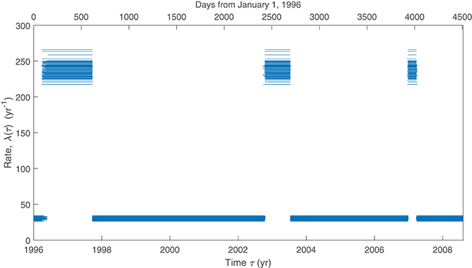
Figure 5. Posterior distribution samples of function λ(τ).
Figure 6 shows posterior modeled periods of high PDC frequency shaded slate blue, with transition times {sm, tm} shown as dark blue lines whose width indicates their uncertainty. Actual observed cumulative PDC event counts are shown as red curve. Interestingly, transition times {sm} from high to low activity appear more precisely determined by the data than those {tm} from low to high. This may, for example, impact decisions on the timing of enlarging no-entry zones when faced with indications of newly heightened activity levels.
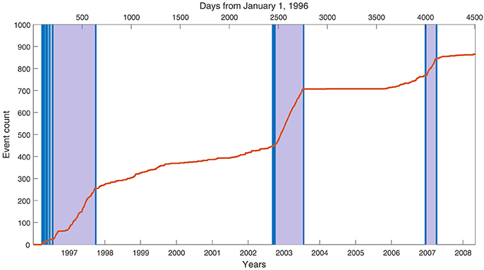
Figure 6. Cumulative event counts as red curve, with posterior high-activity periods indicated by slate blue shading and transition times between activity levels indicated by dark blue lines. Width of dark blue segments indicates posterior uncertainty about transition times. Line slopes correspond to heights in Figure 5.
2.2. A Dynamic Model for PDC Volume and Direction
Here we model the volumes V and initial directions ϕ of PDCs at SHV.
2.2.1. A Dynamic Model for PDC Volumes
Large flow volumes {vj} at Soufrière Hills Volcano are well fit by a power law or Pareto probability model in which the conditional probability that a PDC volume exceeds any value v, given that it exceeds a lower threshold v0, is approximately proportional to a negative power of v:
The near-linearity on the log-log scale plot of frequency-vs.-volume presented in Figure 7 suggests that this holds for α ≈ 1.10 and any (note that α is commonly referred to as the “shape parameter” of the Pareto distribution). Artifacts in the dataset (such as the clumping of reported values at round numbers of 5·106m3 and below) affect reported volumes for smaller flows, making it difficult to confirm or refute relation (7) for lower values of v0. We make the modeling assumption that Equation (7) continues to hold for values of v0 as small as the lower limit of flows reported in Ogburn et al. (2012), 0.15·106m3. We denote this lower limit by ϵ: = 0.15·106m3, and limit our modeling efforts to flows of volume V ≥ ϵ. This assumption makes very little difference in forecasts of flows large enough to be hazardous, e.g., those exceeding 106m3 (which we term “significant”). A generalized likelihood-ratio test gave a GLR of Λ = 3.6·10−30 for Log-Normal distributions compared to Pareto for all 145 recorded PDCs of volume exceeding ϵ and Λ = 4.3 × 10⁻⁷ for the 45 significant PDCs of volume exceeding 1·106m3, overwhelming evidence in favor of the Pareto. Note this contrasts with the results of Neri et al. (2015), who found the evidence about log-normal vs. Pareto inconclusive for a smaller data set and who expressed their own preference for the log-normal.
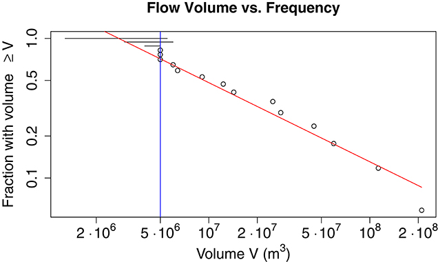
Figure 7. Plot of fraction of PDCs with volume exceeding V, vs. V, on log-log scale, for PDCs of volume V ≥ 5·106m3 (shown as vertical blue line). Near linearity suggests Pareto (power-law) distribution. Measurement artifacts distort entries below about 6·106m3: some small volumes are reported only as ranges, indicated here by horizontal lines, and some small volumes are rounded off, leading to apparent ties in the data.
The Pareto distribution has much heavier tails than do more commonly encountered distributions like the exponential, log-normal, or gamma, i.e., the probability of exceeding high thresholds for Paretos does not decrease as fast as it does for these other distributions. As a consequence, under this Pareto model one is much more likely to observe future volumes that far exceed those in the recent history. For example, if are independent with identical exponential distributions, the probability that a new observation V11 would be ten time higher than the largest max(V1, …, V10) of ten recent ones is about 5·10−6; for Pareto random variables (like ours) with α ≈ 1, it's about 10−2. The probability that V101 is ten times higher than the most recent 100 values max(V1, …, V100) for exponential random variables is about 2·10−14; it's far larger for Pareto random variables, about 10−3.
The evidence against stationarity of PDC volumes, like that against independence of initiation angles and PDC volumes described in section (1), is very weak. Thus, we model PDC volumes {Vj} exceeding threshold ϵ: = 0.15·106m3 as independent and identically-distributed Pa(α, ϵ) random variables, independent of the times {τj} and initiation angles {ϕj}. Note, this modeling choice is the only one shared between this work and our earlier modeling efforts (Bayarri et al., 2009), presenting a simpler stationary model.
2.2.2. Interval Censoring
Some PDC volumes vj are specified precisely in our data set; for others (typically smaller ones), we learn only that vj lies in a reported interval . Such data are said to be “interval censored”. Let J0 be the set of indices for the uncensored observations, let J1 be the index set for censored observations, and let J: = J0 ∪ J1 denote their union, the set indexing all observations. From (7), the likelihood and log likelihood for the Pareto shape parameter α, based on observed values {vj:j ∈ J0} of independent Pareto-distributed random variables representing the volumes of PDCs exceeding ϵ = 0.15·106m3, would be anything proportional to L0 and any constant plus ℓ0, respectively, for:
The precise volumes vj of some (particularly smaller) PDCs in our data, however, are not reported— instead, an interval is reported with the understanding that . Some of these are shown in Figure 7 as horizontal line segments indicating the range of possible values of vj. The likelihood and log likelihood for interval-censored data of this kind are
Combining (8a) (and setting ) for the uncensored volume observations {vj:j ∈ J0}, and (8b) for the censored ones , gives overall log likelihood
reflecting the evidence about α from both censored and uncensored observations. This reflects fully the uncertainty arising from imprecisely reported (i.e., interval censored) volumes.
2.2.3. A Dynamic Model for PDC Angles
Figure 2 suggests that, in the periods between major dome-collapse PDC events, initiation angles {ϕj} are not uniformly distributed on the circle— rather, within those epochs they appear to be concentrated in the vicinity of some central direction, which may change following PDC events large enough to change the dome morphology (often by dome collapse). We take flows exceeding a threshold volume of Ω: = 6·106m3 as surrogates for “dome collapse events”, and model initial flow angles in the epoch (Te, Te+1] between successive major flows of volume V > Ω with von Mises distributions:
(where “” indicates that the {ϕj} are independent with the specified distributions, here the indicated von Mises) for a common concentration parameter κϕ and epoch-specific centrality parameters {μe}. Note that we model the precise direction ϕj of initial dome collapse, but we observe only the valley(s) inundated by the resulting PDC. A Generalized Likelihood Ratio Test comparing the fit to data of a single von Mises distribution for all PDCs, compared to fitting separate von Mises distributions within epochs, generated a χ2 statistic of 214.5 on 20 degrees of freedom, for a p-value of 1.5·10−34, overwhelming evidence against uniformity of the angular distribution across epochs.
The von Mises distribution (von Mises, 1918; Mardia and Jupp, 1999, section 3.5.4) on the circle S1 of possible initiation angles ϕ is governed by two parameters: the central direction μ ∈ S1 and the concentration κ ≥ 0. A concentration of κ = 0 gives the uniform distribution on S1 with no concentration at all, while larger values of κ are more and more concentrated in a small range symmetrically distributed around μ. The probability density function for the vM(μ, κ) distribution (in degrees) with centrality parameter μ ∈ S1 and concentration parameter κ ≥ 0 is given in Equation (10b) (in which I0 denotes the modified Bessel function of order zero; see Abramowitz and Stegun, 1964, section 9.6.16), and is plotted for a few representative values of κ (all centered at μ = 135°) in Figure 8.
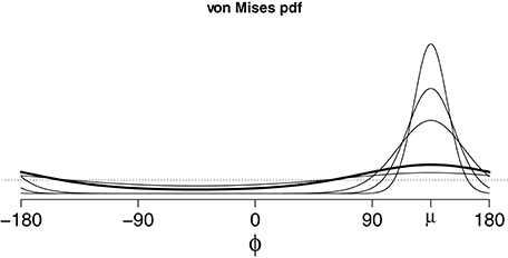
Figure 8. Periodic probability density functions for von Mises distributions centered at μ = 135° (due NW, toward the Belham Valley) with six possible concentration parameters κ ∈ {0, 0.5, 1, 5, 10, 20}. Distribution is more concentrated (with higher peaks at ϕ = μ) for larger κ. Thick line is κ = 1, dotted line is κ = 0 (uniform pdf on S1) for contrast.
Figure 2 suggests that the initial angles of PDC events seem to be centered within particular valleys between successive major events of volume V > Ω = 6·106m3. To explore this phenomenon, we fit a sequence of von Mises vM(μe(τ), κμ) distributions whose centrality parameter μe is a function of time τ.
In an attempt to guide our modeling efforts, we explore von Mises fits to data in intervals between major events. Figure 9, with time on the horizontal axis, shows red vertical bars representing the valleys inundated by major flows, the same valleys shown as red arcs in Figure 2. Angles in the range (−180°, +180°] counter-clockwise from due East (0°) are plotted on the vertical axis. The blue-gray vertical bars represent 95% credible intervals for the von Mises centrality parameters {μe}, fit using Maximum Likelihood estimates based only on the valley data in the time interval (Te, τ] from the previous major event Te up to the current time τ. This estimate is re-fit every time an additional PDC valley record is included as time evolves. Generally, as time progresses the fit to the centrality parameter gets tighter and often happens to coincide with the valley inundated by the next major flow. This agreement is highlighted by the black vertical bars, the 95% credible interval of the centrality parameter at the time Te+1 of the next major event (using all valley data between major PDCs, Te < τ ≤ Te+1), plotted along with (and often on top of) the red bars. The success of the von Mises fits within each epoch bracketed by major events motivates the following modeling choices.
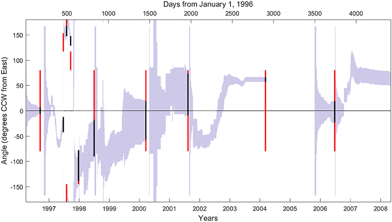
Figure 9. Ninety-five percent credible intervals for centrality parameter μe at each time τ during epoch (Te, Te+1], based only on data in interval (Te, τ]. Predictive distributions for flow directions {ϕj} (not shown) are much wider, reflecting additional uncertainty about how ϕj varies from the center μe of its distribution. Thick black lines indicate 95% intervals for μe at time Te+1 ending this epoch (and beginning the next), while thick red segments indicate valleys inundated by major flow at time Te+1 ending the epoch.
To reflect this phenomenon, we update the centrality parameter μe following the major PDC of volume Vj > Ω at time τj = Te+1 that ends the epoch (Te, Te+1], with a new one:
drawn from another von Mises distribution centered at the old direction μe with its own fixed concentration parameter κμ. The resulting posterior conditional density is:
where N is the number of PDC events {(Vj, ϕj, τj)} and where fPa(v ∣ α, ϵ) and fvM(ϕ ∣ μ, κ) denote the pdfs of the Pa(α, ϵ) and vM(μ, κ) distributions, respectively, evaluated at volume v and direction ϕ.
Here “ej” denotes the epoch e of the jth PDC, which occurs at a time τj satisfying Te < τj ≤ Te+1. The epoch boundaries {Te} and event epochs ej can be calculated from the data {(Vj, ϕj, τj)} by setting T0: = 0 and, for e ∈ ℕ: = {1, 2, 3, … } and j ∈ {1, 2, …, N},
In practice the times τj for all PDC events are observed with adequate precision, but some PDC volumes Vj and initial angles ϕj are not— for some we learn only a range for the volume, and for all we learn only which valley(s) a flow inundated, and not the specific initial angle ϕj, so the data are interval-censored. We accommodate the interval-censored volumes using the approach of section (2.2.2), and the interval-censored angles by integrating each term fvM(ϕj ∣ μej, κϕ) in (10d) with respect to ϕj over the appropriate intervals Φj representing river valley(s) for that flow. Note this approach fully reflects in model forecasts all uncertainty about the precise (but unreported) volumes and angles of flows. Our model for the times and angles of PDCs may be viewed as a self-exciting point process model (i.e., one in which uncertain point intensities are positively correlated at nearby times). Other authors (e.g., Bebbington and Cronin, 2011; Bevilacqua et al., 2016) have used self-exciting point processes to model event locations and times on geological time scales.
Figure 10 shows posterior histograms of PDC central directions {μe} for ten epochs (Te, Te+1]; compare with Figure 2, presenting raw data for the same ten epochs. Figure 11 shows the posterior predictive density function for angles {ϕj} within each epoch (Te, Te+1], as light blue curves, along with the valleys filled by the major PDCs ending those epochs, as shaded intervals.
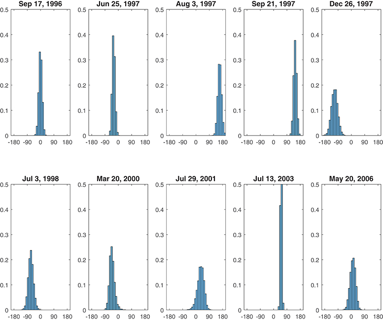
Figure 10. Posterior histograms of epoch-specific central directions {μe}. Each histogram is centered at 0°, due East. Note these are much narrower than prediction histograms for actual angles {ϕj} (cf. Figure 2).
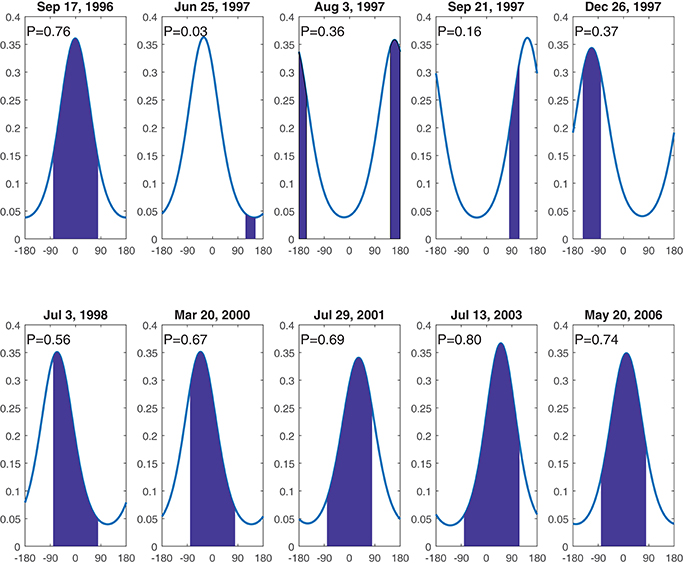
Figure 11. Epoch-specific posterior predictive density functions for PDC initial directions {ϕj}. Area of solid colored band represents the probability (also indicated in the top left of each subplot) for the azimuth range of the valley actually inundated by the next major (Vj > Ω) PDC at epoch-ending time Te+1. Each periodic plot is displayed centered at 0°, due East.
3. Results
3.1. Retrospective Short Term Forecasts
To illustrate how our methods may be used to make short-term forecasts, and to validate those forecasts, we select a specific time in our data set (1st January 2006, a decade into the eruption) and compare model forecasts for the next few years based only on data prior to that date with actual observations from those same years.
Figure 12 shows 100 forecasts of cumulative PDC volume from 1st January 2006 to 1st August 2008 (just over 2.5 years), all based on eruption data prior to 2006. Solid black symbols show the actual cumulative PDC volume then observed in that forecast interval, exhibiting eruption rates and jump sizes similar to those in model forecasts. This may be viewed as a validation of our forecast approach: forecasts of “future” collapse frequencies within the existing data set, based on prior data, are broadly consistent with observations of what actually occurred. For example, the central 90% predictive forecast interval for cumulative volumes after 180 days is 4–250·106m3, and the actual cumulative volume at that date was 120·106m3; the central 90% predictive interval for the highest-volume PDC (and so the biggest jump) in the first year is 2.2–350·106m3, while the largest observed PDC volume is 200·106m3.
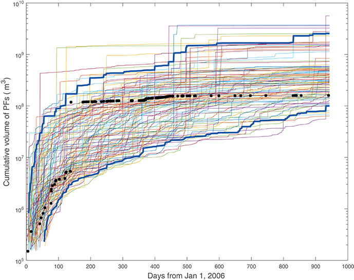
Figure 12. Forecast activity, with data overlaid. Shows 100 forecasts of cumulative PDC volume in the period from 1st January 2006 to 1st August 2008, forecast using prior data. Asterisk symbols “*” show realized cumulative volume. Thick blue lines show pointwise 90% prediction intervals.
Figure 13 shows the forecast activity levels λ(t), cumulative event counts, central directions {μe} (counter-clockwise from due East), and cumulative volumes in Figures 13A–D, respectively, from a single draw from the posterior predictive distribution of activity from 1st January 2006 through 1st August 2008. Note that during time intervals of high frequency λ(t) (as indicated in Figure 13A), PDC event frequencies in Figure 13B are higher (i.e., cumulative event count slope is steeper), and density of points is higher in Figures 13C,D. Also note that change times for centrality parameters μe in Figure 13C coincide with major jumps in cumulative volume Figure 13D), i.e., with large-volume PDCs.
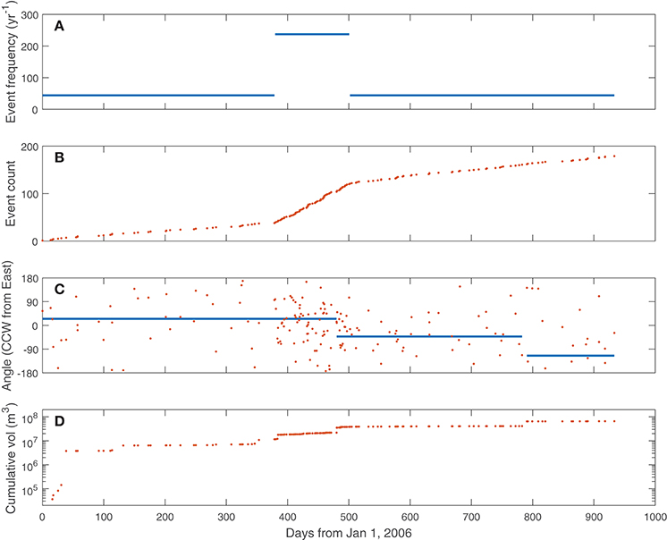
Figure 13. One posterior draw of simulated forecast PDC activity for the period from 1st January 2006 to 1st August 2008 (943 days), forecast using prior data. Top panel (A) shows expected frequency λ(t) of PDC events. Second panel (B) shows cumulative event counts. Third panel (C) shows forecast central directions {μe} as solid blue curve and individual PDC events as red dots. Bottom panel (D) shows cumulative volume.
Figure 14 offers another way of visualizing the same posterior predictive simulation presented in Figure 13. Time (in days) is represented radially on a linear scale. Central angles {μe} are represented as radial line segments that may change at the times (indicated by concentric circles) of dome-collapse PDCs, whose angles are indicated by filled colored circles. This draw featured two such major PDCs, and so two full epochs and part of a third, in that first approximately 2.5 years.
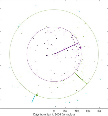
Figure 14. Same posterior draw of forecast PDC activity as in Figure 13, for the period of 1st January 2006 through 1st August 2008. Time in days since 1st January 2006 is shown radially on linear scale. Colored radial segments indicate central directions {μe}, which change at epoch-ending times τj = Te of events (indicated by concentric circles, with direction of major flows shown as filled circles). Individual PDC events are shown as colored dots.
Probability forecasts based on Monte Carlo simulations of PDCs (i.e., repeatedly sampling volumes Vj, times τj, and initiation angles ϕj as illustrated in Figures 12, 13), based on the posterior distributions described in this work, quantify both epistemic and aleatoric uncertainty—let us explain further. Note that in Figures 5, 10 that there is not one single “right” value of λlo, λhi, or {μe}, but for each of these parameters there is a distribution of possible values, some more likely than others. This is also true for the Pareto shape parameter α (the negative slope of the log-log volume distribution intended to model the data in Figure 1). In the Bayesian paradigm, such distributions of parameters reflect the epistemic uncertainty resulting from the fact that these models (and parameters) are fit using a limited quanity of imperfect data. Each thin colored curve in Figure 12 has its own sample values of λlo, λhi, and α, that specify the Poisson and Pareto distributions used to sample PDC event times and volumes. Each thin colored curve in the cumulative volume forecast is then calculated by summing up (sampled) PDC volumes at the (sampled) times they occur. This idea is perhaps easier to see in Figure 13. The solid blue lines in the panels represent samples from parameter probability distributions (frequencies in the top panel, central angles in the third panel). The orange dots are various PDC samples over time. Together the panels in Figure 13 represent one realization of a PDC forecast. A different realization would have both different parameter samples (blue curves) and PDC samples (orange dots).
Aleatoric uncertainty describes the natural randomness of a system, so modeling the system probabilistically is the first step to quantifying aleatoric uncertainty. Our modeling approach lets us take this one step further to incorporate information about the current state of the system. That is, we can begin a probability forecast in either a state of high or low PDC frequency, chosen to match the current (at the beginning of the forecast period) level of activity available from monitoring data. Likewise, we can begin a forecast where the central angle μ0 is set to reflect the current dome alignment. The later case leads to dramatic differences in short-term forecasts, as illustrated in Figure 15. In either case if we were to forecast over longer time horizons, say years, the effects of non-stationary modeling would wash out. That is, the system would naturally evolve away from its initial state (high or low frequency, initial dome alignment, etc.) making probability forecasts much less sensitive to assumptions about the initial state of the system. This illustrates the importance of both non-stationary probabilistic modeling and potential incorporation of monitoring data into short term forecasts.
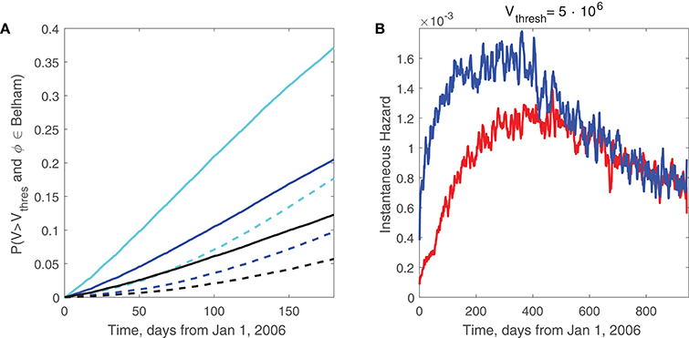
Figure 15. (A) forecast probability of a PDC inundating the Belham Valley with a volume exceeding threshold Vthresh in first t days following 1st January 2006, vs. t, for a dome facing the Tar valley (due East, , typical for SHV dome in 2000), as dashed curves; and for a dome facing the Belham Valley (Northwest, , typical for 2018), as solid curves. Threshold volume Vthresh is 2·106m3 for cyan curves, 5·106m3 for blue curves, and 10·106m3 for black curves. Forecasts are based only on data prior to 1st January 2006. (B) forecast daily hazard of Belham inundation by a flow exceeding 5·106m3 for a longer period, for a dome facing the Belham (), as upper blue curve, and for a dome facing due East (), as lower red curve. Note hazards differ strikingly for first 200 days but are indistinguishable after 600 days. Daily (or instantaneous) hazard is the probability of inundation on day t, conditional on having no earlier inundation.
Figure 15A shows the forecast probability of large flows (V > Vthresh for Vthresh = 2, 5, or 10·106m3) down the azimuth sector covered by the Belham valley in the first t days following 1st January 2006, based on data prior to 2006, for two possible dome orientations suggested by monitoring information: one facing due East toward the Tar valley, , typical for SHV in 2000 (the lower dashed curves); and one facing Northwest toward the Belham valley, , typical for SHV in 2018 (the upper solid curves). This illustrates how easily changing conditions can be reflected in model forecasts in this modeling approach, and how they affect forecasts.
Figure 15B shows daily hazard, the probability of Belham Valley inundation on the tth day after 1st January 2006 conditionally on no prior inundation. For , at t = 180d the probability is about 1.5·10−3/d if the initial dome faces the Belham valley (), notably higher than the value 1.0·10−3/d if the initial dome faces the Tar River valley (). By t = 600d there is no difference in hazard— it is approximately 1.1·10−3/d for both and . This illustrates how the present methodology is capable of supporting short-term forecasts that reflect current conditions, unlike models embodying stationary assumptions.
Although Figures 12, 15 both present forecasts, they are different in nature and it is worth contrasting them. The information presented in Figure 12 about cumulative volumes (model samples, confidence intervals, and data) provides a validation of sorts—the data (black asterisks) look much like a sample from our model (colored curves). In Figure 15 we present probability forecasts and instantaneous hazard curves conditioned on a current state of the volcano (dome growth direction) that could be informed by monitoring data. This kind of short-term forecasting, that can be readily updated as new data become available or as the system evolves, is how we imagine such modeling efforts will be utilized by volcanologists, observatories, and civil protection authorities.
4. Discussion and Conclusions
Statistical modeling assumptions based on stationarity are reasonable for long-time pyroclastic density current forecasting (5–10 years), but they are neither reasonable nor consistent with data over short time scales (days–months). In this work, we introduce models for frequency, volume, and initial direction of pyroclastic density currents that can capture non-stationary and heavy-tailed behavior consistent with the data at SHV. The data clearly contain periods of high and low frequency of flows associated with phases of dome growth and extrusion pauses. This is consistent with geological observations that as a given lava lobe extrudes, PDCs are generated around that locus of activity but after a significant dome collapse, subsequent new growth may occur on a different part of the dome (Calder et al., 2002).
Furthermore, the directional data show that sequential small flows tend to inundate the same or adjacent valleys and that they tend to precede a moderately large to large flow with a similar orientation, after which the dominant direction may change.
Our statistical modeling assumptions are simple and, importantly, are not tied to geological observations or explanations, yet are consistent with the behavior of the data. Our model allows the system to change from a high-to-low or low-to-high frequency at random times. It allows the directions (or valleys) of successive flows to vary randomly yet have a shared preference. It also allows this shared preference to be re-set after each major pyroclastic density current. In addition, our volume model indicates that we are in a heavy-tailed regime where larger-than-recorded events must be accounted for in forecasting. This is a key outcome, which is critically important for volcanic hazard assessment. We employ the Bayesian paradigm for inference and forecasting, which provides a coherent mechanism to account for uncertainty about both model fit (epistemic uncertainty, arising from our imprecise knowledge of model parameters and the imperfect fit of the model to nature) and forecasts (which must also reflect aleatoric uncertainty, or the natural variability of geophysical systems). Data constrain this model well, and retrospective forecasts are consistent with the data.
We believe that the power of this modeling framework lies in its ability to support updating short-term forecasts during periods of rapidly changing activity. (Note that this or a similar framework could be applied to other active volcanic systems, other volcanic hazard types, or to other natural hazards.) That is, we can condition forecasts on the knowledge that we are currently in a period of high-activity (or low-activity), but still account for the fact that there is a significant chance of transition between those levels during the forecast interval. Likewise, we can make short-term forecasts based on other readily observable traits of the system (e.g., dome growing toward east vs. dome growing toward northwest). The fact that our model also accounts for epistemic uncertainty is critical for hazard assessment as quantitative analysis of data is necessary for fully defensible decision making (Bretton and Aspinall, 2017).
Probabilistic volcanic hazard maps such as those developed in Connor et al. (2012); Volentik and Houghton (2015); Biass et al. (2016); Mead and Magill (2017) represent the state of the art in volcanic hazard assessment. Each of these works combines probabilistic scenario models and physical simulations of potentially hazardous volcanic processes (lava flows, lahars, and tephra fallouts, respectively). However, the computational expense of exercising a physical model at a large number of samples from a scenario model is often a limiting factor in constructing a probabilistic assessment. This typically has the result that a probabilistic hazard map needs to “settle” for a single scenario distribution.
Looking forward, modeling efforts like those presented here provide additional flexibility. In particular, they may be even more powerful when used in conjunction with complex geophysical models, and in simulations of pyroclastic density currents to make short-term probabilistic hazard maps. Probabilistic hazard maps for pyroclastic density currents display probabilities of inundation spatially in potentially vulnerable areas surrounding a volcano (Bayarri et al., 2009, 2015; Spiller et al., 2014). These works introduce an efficient approach to combine scenario and physical models that results in the rapid construction of probabilistic hazard maps that enable the exploration of various aleatoric scenarios. Short-term probabilistic hazard maps, constructed this way, would allow one to visualize the change in hazard threat as scenario models are updated.
Author Contributions
RW: did most of the model development, derived likelihood and posterior distributions, oversaw the continuing development of the model as it evolved, did some of the computer coding. ES: significant contributions to model development, most of the computer coding and figure generation, significant contributions to model evolution. EC: motivated entire project; supplied the needed expertise in geology and volcanology, supplied the data, helped ensure the model's consistency with geophysical processes.
Conflict of Interest Statement
The authors declare that the research was conducted in the absence of any commercial or financial relationships that could be construed as a potential conflict of interest.
Acknowledgments
The authors would like to thank Sarah E. Ogburn, lead developer of the DomeHaz database (Ogburn et al., 2012), for help in acquiring and interpreting the data used in this study, and Pablo Tierz Lopez for helpful conversations. This work was supported by U.S. National Science Foundation grants EAR-0809543, DMS-1741377, DMS-1741291, DMS-1622403, DMS-1621853, and SES-1521855. Any opinions, findings, and conclusions or recommendations expressed in this material are those of the authors and do not necessarily reflect the views of the NSF.
References
Abramowitz, M., and Stegun, I. A. (eds.). (1964). Handbook of Mathematical Functions With Formulas, Graphs, and Mathematical Tables, Vol 55 of Applied Mathematics Series. Washington, DC: National Bureau of Standards.
Aspinall, W. P., Woo, G., Voight, B., and Baxter, P. J. (2003). Evidence-based volcanology: application to eruption crises. J. Volcanol. Geoth. Res. 128, 273–285. doi: 10.1016/S0377-0273(03)00260-9
Bayarri, M. J., Berger, J. O., Calder, E. S., Dalbey, K., Lunagómez, S., Patra, A. K., et al. (2009). Using statistical and computer models to quantify volcanic hazards. Technometrics 51, 402–413. doi: 10.1198/TECH.2009.08018
Bayarri, M. J., Berger, J. O., Calder, E. S., Patra, A. K., Pitman, E. B., Spiller, E. T., et al. (2015). Probabilistic quantification of hazards: A methodology using small ensembles of physics based simulations and statistical surrogates. Int. J. Uncertain. Quantif. 5, 297–339. doi: 10.1615/Int.J.UncertaintyQuantification.2015011451
Bebbington, M. S. (2007). Identifying volcanic regimes using Hidden Markov Models. Geophys. J. Int. 171, 921–942. doi: 10.1111/j.1365-246X.2007.03559.x
Bebbington, M. S. (2010). Trends and clustering in the onsets of volcanic eruptions. J. Geophys. Res. 115, 1–13. doi: 10.1029/2009JB006581
Bebbington, M. S. (2012). Models for temporal volcanic hazard. Stat. Volcanol. 1, 1–24. doi: 10.5038/2163-338X.1.1
Bebbington, M. S., and Cronin, S. J. (2011). Spatio-temporal hazard estimation in the Auckland Volcanic Field, New Zealand, with a new vent-order model. Bull. Volcanol. 73, 55–72. doi: 10.1007/s00445-010-0403-6
Berger, J. O., Bernardo, J. M., and Sun, D. (2009). The formal definition of reference priors. Ann. Statist. 37, 905–938. doi: 10.1214/07-AOS587
Bevilacqua, A., Flandoli, F., Neri, A., Isaia, R., and Vitale, S. (2016). Temporal models for the episodic volcanism of Campi Flegrei caldera (Italy) with uncertainty quantification. J. Geophys. Res. 121, 7821–7845. doi: 10.1002/2016JB013171
Bevilacqua, A., Neri, A., Bisson, M., Ongaro, T. E., Flandoli, F., Isaia, R., et al. (2017). The effects of vent location, event scale, and time forecasts on pyroclastic density current hazard maps at Campi Flegrei caldera (Italy). Front. Earth Sci. 5:72. doi: 10.3389/feart.2017.00072
Biass, S., Bonadonna, C., Connor, L., and Connor, C. (2016). TephraProb: a Matlab package for probabilistic hazard assessments of tephra fallout. J. Appl. Volcanol. 5, 1–16. doi: 10.1186/s13617-016-0050-5
Bretton, R., and Aspinall, W. (2017). Natural hazards: risk assessments face legal scrutiny. Nature 550, 188–188. doi: 10.1038/550188b
Calder, E. S., Luckett, R., Sparks, S. J., and Voight, B. (2002). “Mechanisms of lava dome instability and generation of rockfalls and pyroclastic flows at Soufrière Hills Volcano, Montserrat,” in The Eruption of Soufrière Hills Volcano, Montserrat from 1995 to 1999, Number 21 in Geological Society Memoirs, eds T. H. Druitt and B. P. Kokelaar (London, UK: London Geological Society), 173–190.
Carta, S., Figari, R., Sartoris, G., Sassi, E., and Scandone, R. (1981). A statistical model for vesuvius and its volcanological implications. Bull. Volcanol. 44, 129–151. doi: 10.1007/BF02597700
Charbonnier, S. J., and Gertisser, R. (2012). Evaluation of geophysical mass flow models using the 2006 block-and-ash flows of Merapi Volcano, Java, Indonesia: towards a short-term hazard assessment tool. J. Volcanol. Geother. Res. 231–232, 87–108. doi: 10.1016/j.jvolgeores.2012.02.015
Connor, L. J., Connor, C. B., Meliksetian, K., and Savov, I. (2012). Probabilistic approach to modeling lava flow inundation: a lava flow hazard assessment for a nuclear facility in Armenia. J. Appl. Volcanol. 1, 1–19. doi: 10.1186/2191-5040-1-3
Hinks, T. K., Komorowski, J.-C., Sparks, R. S. J., and Aspinall, W. P. (2014). Retrospective analysis of uncertain eruption precursors at La Soufrière volcano, Guadeloupe, 1975–77: volcanic hazard assessment using a Bayesian Belief Network approach. J. Appl. Volcanol. 3, 1–26. doi: 10.1186/2191-5040-3-3
Jaquet, O., Lantuejoul, C., and Goto, J. (2017). Probabilistic estimation of long-term volcanic hazard under evolving tectonic conditions in 1 Ma timeframe. J. Volcanol. Geoth. Res. 345, 58–66. doi: 10.1016/j.jvolgeores.2017.07.010
Karlin, S., and Taylor, H. M. (1975). A First Course in Stochastic Processes. New York, NY: Academic Press.
Marzocchi, W., Sandri, L., and Selva, J. (2008). BET_EF: a probabilistic tool for a long- and short-term eruption forecasting. Bull. Volcanol. 70, 623–632. doi: 10.1007/s00445-007-0157-y
Mead, S. R., and Magill, C. R. (2017). Probabilistic hazard modelling of rain-triggered lahars. J. Appl. Volcanol. 6, 1–7. doi: 10.1186/s13617-017-0060-y
Neri, A., Bevilacqua, A., Ongaro, T. E., Isaia, R., Aspinall, W. P., Bisson, M., et al. (2015). Quantifying volcanic hazard at Campi Flegrei caldera (Italy) with uncertainty assessment: 2. Pyroclastic density current invasion maps. J. Geophys. Res. 120, 2330–2349. doi: 10.1002/2014JB011776
Ogburn, S. E., Loughlin, S. C., and Calder, E. S. (2012). DomeHaz: Dome-Forming Eruptions Database. Available online at https://vhub.org/groups/domedatabase
Rosenthal, J. S. (2011). “Optimal proposal distributions and adaptive MCMC,” in Handbook of Markov Chain Monte Carlo, eds S. Brooks, A. Gelman, G. L. Jones, and X.-L. Meng (Boca Raton, FL: Chapman and Hall), 93–112.
Sandri, L., Guidoboni, E., Marzocchi, W., and Selva, J. (2009). Bayesian event tree for eruption forecasting (BET_EF) at Vesuvius, Italy: a retrospective forward application to the 1631 eruption. Bull. Volcanol. 71, 729–745. doi: 10.1007/s00445-008-0261-7
Sandri, L., Thouret, J.-C., Constantinescu, R., Biass, S., and Tonini, R. (2014). Long-term multi-hazard assessment for El Misti volcano (Peru). Bull. Volcanol. 76, 1–26. doi: 10.1007/s00445-013-0771-9
Spiller, E. T., Bayarri, M. J., Berger, J. O., Calder, E. S., Patra, A. K., et al. (2014). Automating emulator construction for geophysical hazard maps. J. Uncertain. Quantif. 2, 126–152. doi: 10.1137/120899285
Sulpizio, R., Capra, L., Sarocchi, D., Saucedo, R., Gavilanes-Ruiz, J. C., and Varley, N. R. (2010). Predicting the block-and-ash flow inundation areas at Volcáne Colima (Colima, Mexico) based on the present day (February 2010) status. J. Volcanol. Geother. Res. 193, 49–66. doi: 10.1016/j.jvolgeores.2010.03.007
Volentik, A. C. M., and Houghton, B. F. (2015). Tephra fallout hazards at Quito International Airport (Ecuador). Bull. Volcanol. 77, 1–14. doi: 10.1007/s00445-015-0923-1
von Mises, R. (1918). Über die “Ganzzahligkeit” der Atomgewicht und verwandte Fragen. Physikalische Z. 19, 490–500.
Wadge, G., Herd, R. A., Ryan, G., Calder, E. S., and Komorowski, J.-C. (2010). Lava production at Soufrière Hills Volcano, Montserrat: 1995–2009. Geophys. Res. Lett. 37:L00E03. doi: 10.1029/2009GL041466
Woo, G. (2018). Stochastic modeling of past volcanic crises. Front. Earth Sci. 6:1. doi: 10.3389/feart.2018.00001
Keywords: dynamic, forecast, objective Bayesian, Pareto, von Mises, probabilistic, pyroclastic
Citation: Wolpert RL, Spiller ET and Calder ES (2018) Dynamic Statistical Models for Pyroclastic Density Current Generation at Soufrière Hills Volcano. Front. Earth Sci. 6:55. doi: 10.3389/feart.2018.00055
Received: 26 December 2017; Accepted: 24 April 2018;
Published: 23 May 2018.
Edited by:
Victoria Miller, The University of the West Indies St. Augustine, Trinidad and TobagoReviewed by:
Andrea Bevilacqua, University at Buffalo, United StatesMicol Todesco, Istituto Nazionale di Geofisica e Vulcanologia, Italy
Copyright © 2018 Wolpert, Spiller and Calder. This is an open-access article distributed under the terms of the Creative Commons Attribution License (CC BY). The use, distribution or reproduction in other forums is permitted, provided the original author(s) and the copyright owner are credited and that the original publication in this journal is cited, in accordance with accepted academic practice. No use, distribution or reproduction is permitted which does not comply with these terms.
*Correspondence: Robert L. Wolpert, cmx3QGR1a2UuZWR1