Differing Climatic Mass Balance Evolution Across Svalbard Glacier Regions Over 1900–2010

Möller, Marco; Kohler, Jack

doi:10.3389/feart.2018.00128

ORIGINAL RESEARCH article

Front. Earth Sci., 06 September 2018
Sec. Cryospheric Sciences
Volume 6 - 2018 | https://doi.org/10.3389/feart.2018.00128

Differing Climatic Mass Balance Evolution Across Svalbard Glacier Regions Over 1900–2010

Marco Möller^1,2,3^*

Jack Kohler⁴

¹Institute of Geography, University of Bremen, Bremen, Germany
²Geography Department, Humboldt Universität zu Berlin, Berlin, Germany
³Department of Geography, RWTH Aachen University, Aachen, Germany
⁴Norwegian Polar Institute, Tromsø, Norway

Relatively little is known about the glacier mass balance of Svalbard in the first half of the twentieth century. Here, we present the first century-long climatic mass balance time series for the Svalbard archipelago. We use a parameterized mass balance model forced by statistically downscaled ERA-20C data to model climatic mass balance for all glacierized areas on Svalbard with a 250 m resolution for the period 1900–2010. Results are presented for the archipelago as a whole and separately for nine different subregions. We analyze the extent to which climatic mass balance in the different subregions mirror the temporal evolution of the climate warming signal, especially during the early twentieth century Arctic warming episode. The spatially averaged mean annual climatic mass balance for all Svalbard is balanced at −0.002 m w.e. with an associated mean equilibrium line altitude of 425 m a.s.l. When also taking calving fluxes into account, this status leads to an archipelago-wide cumulative mass balance of −16.9 m w.e. over the study period, equaling a sea level equivalent of ~1.6 mm. The long-term evolution of climatic mass balance is largely governed by ablation variability. Refreezing contributes 34% to the archipelago-wide mass gain on average. Considerable variability is evident across Svalbard, with predominantly positive climatic mass balances in the northeastern parts of the archipelago and mostly negative ones in the western and southern parts. The archipelago-wide climatic mass balance shows a statistically significant trend of −0.021 m w.e. per decade and the associated equilibrium line altitude rises with a likewise significant trend of +3.0 m a.s.l. per decade. Spatial variability of the equilibrium line is such that the lowest altitudes are reached across the eastern islands of the archipelago and the highest ones in the central parts of Spitsbergen.

Introduction

Global air temperatures have been continuously increasing over the twentieth century and beyond (Parker, 2011). Due to the Arctic amplification (Serreze and Barry, 2011), this increase is particularly pronounced in the northern polar regions, with significant overall increases over the entirety of the last century (Polyakov et al., 2003) and especially in recent decades (Przybylak, 2007). Only during ~1940–1960 was the process of Arctic warming briefly interrupted by a period of decreasing air temperatures. This, however, followed a major climate anomaly known as the early twentieth century Arctic warming (~1920–1940; Wood and Overland, 2010; Yamanouchi, 2011), during which Arctic air temperatures increased by about 1.7°C on average (Bengtsson et al., 2004).

Glacier retreat on a global scale, in response to the temperature increase, is well-documented (Leclercq et al., 2014). Glaciers and ice caps around the world have experienced increasingly negative mass balance over the second half of the twentieth century (Kaser et al., 2006; Marzeion et al., 2012). However, studies on glacier evolution over the entire twentieth century are scarce and mostly limited to individual glaciers (Möller and Schneider, 2008; Huss et al., 2010; Fettweis et al., 2017).

In the Arctic, the region experiencing the strongest air temperature increases, past glacier evolution has mostly only been described and analyzed since the middle of the twentieth century (Dowdeswell et al., 1997). Even for the Svalbard archipelago (Figure 1), which is among the most intensively studied parts of the Arctic realm, only one century-long mass balance reconstruction [for Werenskiöldbreen by Grabiec et al. (2012)] exists so far. Apart from that, several shorter modeled mass-balance time series exist for individual glaciers on the archipelago (e.g., Rasmussen and Kohler, 2007; Rye et al., 2010; Van Pelt et al., 2012; Möller et al., 2013) as well as for entire Svalbard (Lang et al., 2015; Aas et al., 2016; Möller et al., 2016b; Østby et al., 2017). In situ mass balance measurements on selected glaciers exist for more than four decades, e.g., on Austre Brøggerbreen since 1967 (Bruland and Hagen, 2002). Reflecting the recent air temperature development (Figure 2), all these studies draw a consistent picture of negative mass balance trends across the archipelago and predominantly negative annual balances at most of the modeled and observed glaciers in recent years. This is in accordance with remote sensing-based observations over recent decades, which likewise show glacier retreat and mass losses (Kohler et al., 2007; Moholdt et al., 2010a,b; Nuth et al., 2010, 2013; Jacob et al., 2012; James et al., 2012) over most of Svalbard. Detailed knowledge about glacier evolution from the first half of the twentieth century is, nevertheless, scarce. Mapping of the Vestfonna ice cap (cf. Figure 1) in the early 1930s suggests significant retreat has been ongoing over the entire century. While Ahlmann (1933) documented a surface extent of ~2,810 km² for the ice cap, it shrank to ~2,340 km² in recent years (Braun et al., 2011). Glaciers in southern Svalbard have experienced strong frontal retreat and surface lowering over much of the twentieth century (Pälli et al., 2003).

FIGURE 1

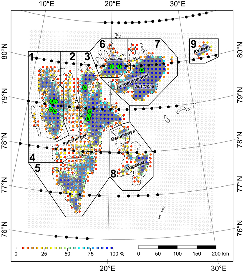
Figure 1. Overview map of Svalbard and its glaciers (shown in gray). The nine different subregions of the archipelago are delineated by thick black lines and numbered by Arabic numerals. Regularly gridded circles indicate locations of RCM grid points, which also form the model domain grid. Glacier grid points are shown with a color code indicating the percentage of glacier coverage in a 10 × 10 km area around each grid point. ERA-20C grid points are indicated by black dots. Only grid points that are used during downscaling are shown. Locations of firn cores used for model validation are indicated by lowercase letters in green circles, corresponding to the names used in Table 1. Names of the main islands of the archipelago are given in bold italics and those of individual glaciers and ice caps mentioned in the text in regular italics.

FIGURE 2

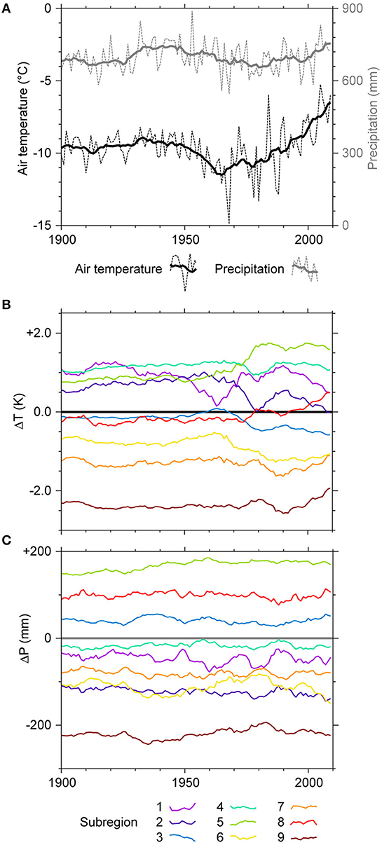
Figure 2. Annual mean air temperature and total precipitation across the Svalbard archipelago over the mass-balance years 1900/1901–2009/2010. (A) Archipelago wide values (thin dashed lines) are shown along with running decadal means (thick lines). Running decadal means for (B) air temperature and (C) precipitation within the nine different subregions (color code) are shown as deviations to the archipelago wide mean (thick black/gray line). The time series are based on downscaled ERA-20C data, averaged over all glacier relevant grid points of the model domain within the respective subregion (cf. Figure 1).

In this paper a degree-day based mass balance model is forced by spatially-distributed, statistically downscaled data from the ECMWF twentieth century reanalysis (ERA-20C; Poli et al., 2016) to obtain the first mass balance time series for all glacierized areas of the Svalbard archipelago for the entire twentieth century. The aim of this paper is to analyze to which extent glacier mass balance evolution within nine different subregions of Svalbard (cf. Figure 1; Table 1) follows the climate warming over the century, to see whether spatial or temporal differences in glacier mass balance evolution exist. Finally, a trend analysis is performed to investigate if the mass balance evolution across the archipelago and in the subregions is homogeneous.

TABLE 1

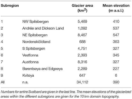
Table 1. Key numbers of the nine subregions of Svalbard (cf. Figure 1).

Study Area

The European Arctic archipelago Svalbard (Figure 1) is covered by 33,775 km² of glaciers (Nuth et al., 2013). These ice masses comprise the large ice caps on Nordauslandet and Kvitøya and extensive ice fields in most parts of the archipelago's main island, Spitsbergen, and on Barentsøya and Edgeøya. Only the central parts of Spitsbergen are dominated by small cirque and valley glaciers. Most of the drainage from the larger ice caps and ice fields occurs through tidewater glaciers, a considerable number of which are surge type (Błaszczyk et al., 2009).

The archipelago is situated north of the European mainland halfway to the North Pole between the northern Atlantic Ocean to the south and the Arctic Ocean to the north. Marked temperature differences between the various influencing ocean currents and air masses thus shape the climate of Svalbard. While the western part of the archipelago is mostly influenced by the warm West Spitsbergen Current (Walczowski and Piechura, 2011), distinctly cooler waters from the Arctic Ocean reach the eastern part (Loeng, 1991). Also the dominant air masses are either relatively warm and humid Atlantic air or cold and dry Arctic air (Svendsen et al., 2002).

Annual air temperature on Svalbard has a positive trend over most of the twentieth century (Nordli et al., 2014), apart from the cold ~1940–1970 period. However, trends are only statistically significant since the 1970s with a strong climate warming of ~1°C per decade (Førland et al., 2011). Similarly to air temperature, precipitation also shows a significantly positive trend of ~2% per decade over the twentieth century (Førland et al., 2011).

Data and Methods

General Approach

To model twentieth century glacier mass balance we use a degree-day based climatic mass balance (CMB) model. Climatic mass balance is the sum of ablation, accumulation and all refreezing (Cogley et al., 2011). The CMB model is forced by downscaled air temperature and precipitation reanalysis data and delivers output on daily time steps over a study period covering the mass balance years 1900/1901–2009/2010, i.e., the period from 1 September 1900 to 31 August 2010. This output is used to calculate reference-surface mass balances (Elsberg et al., 2001), i.e., mass balances based on a time-invariant glacier extent; here we use the 2001–2010 geometry given in the Glacier Area Outlines-Svalbard inventory (Nuth et al., 2013). Spatial distribution during modeling across all glacierized areas of the Svalbard archipelago (Figure 1) is realized on a 250 m resolution model domain. The 250 m topography is derived by resampling the 50 m resolution digital elevation model Terrengmodell Svalbard (S0 Terrengmodell) provided by the Norwegian Polar Institute (2014).

Climate-Data Downscaling

Overall Basics

To generate the input climate data, synoptic-scale reanalysis data are adjusted to local conditions across Svalbard using a two step procedure (Figure 3). The synoptic scale is represented by air temperature and precipitation data from the ECMWF twentieth century reanalysis (ERA-20C; Poli et al., 2016), which are given on a 1.0° resolution (Figure 1). We do not rely on the Twentieth Century Reanalysis Project [20CR; Compo et al. (2011)], as initial tests showed that this dataset does not adequately reproduce the observed positive precipitation trend on Svalbard over the twentieth century (cf. section Study Area).

FIGURE 3

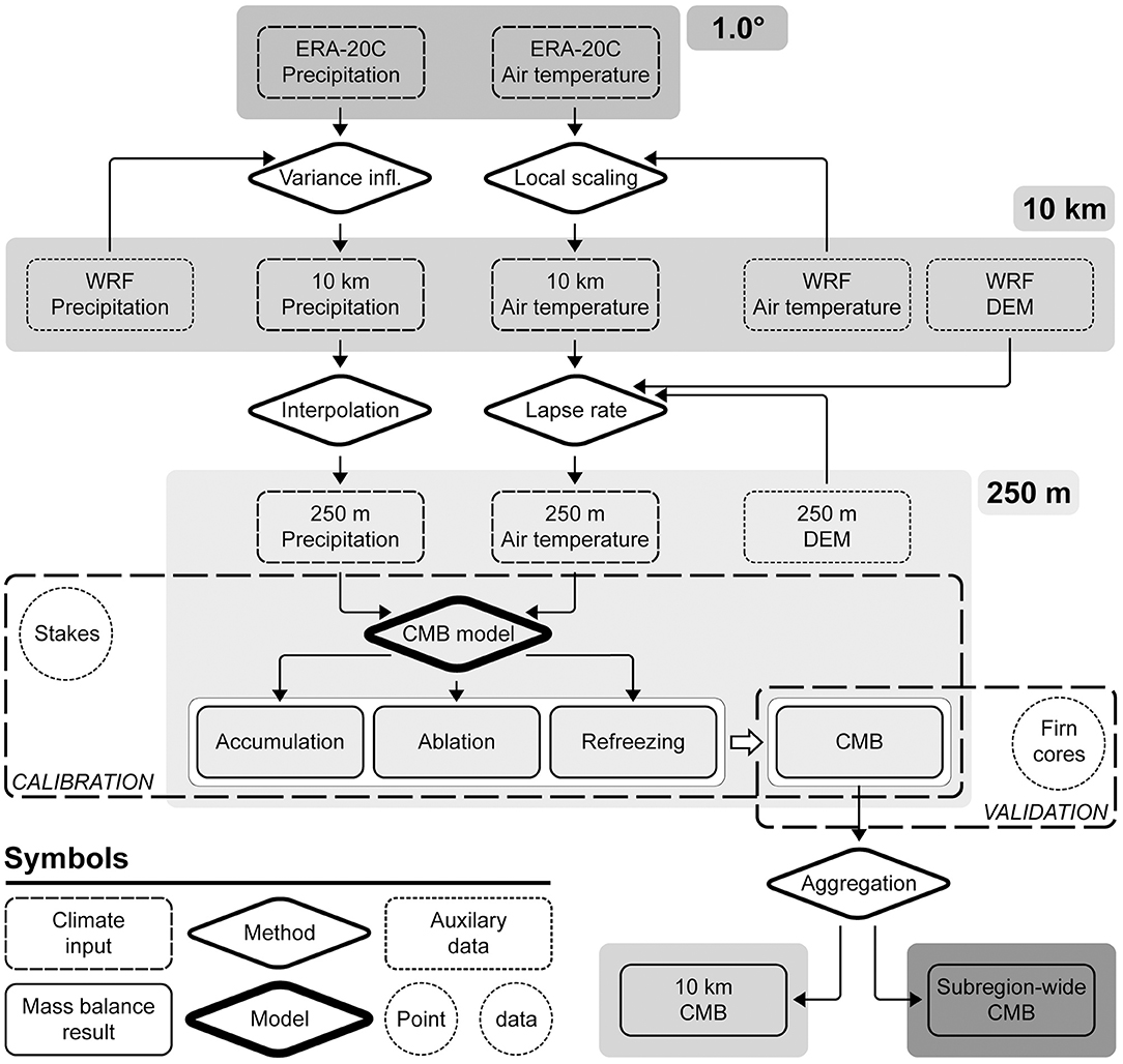
Figure 3. Workflow during climate data downscaling and climatic mass balance (CMB) modeling. Different levels of spatial resolution are indicated by gray shading in the background. Details on climate input data or any auxiliary data are given in section Climate-Data Downscaling. Details on calibration of the CMB model and validation of the results are given in section Mass-Balance Modeling. The aggregation of the daily CMB fields produced by the CMB model to 10 km resolution fields is done in preparation for Figure 10, while the aggregation to subregion-wide CMB is done for all other tables and figures which report on the results.

The first step of downscaling leads to an intermediate scale domain with a 10 km resolution. The second step of downscaling leads to the final model domain with a 250 m resolution. Both of these steps are carried out separately for each individual, glacier-relevant grid point of the 10 km domain. In total, 694 10 km grid points contain glacierized areas within the area they represent and are thus considered as glacier relevant (cf. Figure 1).

As in situ reference for the downscaling we consider 10 km scale output from the Polar Weather Research and Forecast (WRF) model (version 3.1.1; cf., Hines and Bromwich, 2008). This reference is given in the form of daily air temperature and precipitation fields (Finkelnburg, 2013; Figure 1), which have already been successfully applied in glaciological modeling on Svalbard (Sauter et al., 2013; Möller et al., 2016a,b). Along with the climate data, the WRF dataset provides elevation information for each grid point which resembles the median elevation of the 50 m Norwegian Polar Institute (2014) DEM within a 10 × 10 km area centered at the respective WRF grid point. However, on the island Kvitøya the WRF elevations are far lower which suggests them to be erroneous.

In the first step of downscaling, time series of the four ERA-20C grid points directly surrounding the respective 10 km domain grid point are included. A comparable approach has already been used in downscaling global circulation model air temperature and precipitation data (Möller et al., 2016a). By following this approach, the spatial variability of climate conditions across the archipelago, which is well-represented in the WRF fields, is implicitly transferred to the downscaled ERA-20C air temperature and precipitation fields. Compared to purely statistical downscaling, this hybrid approach is able to reproduce spatial variability resulting from dynamic effects like e.g., orographic precipitation. The years in which the WRF fields and ERA-20C data overlap (2000–2010) were used as a reference period for downscaling.

The second step of downscaling leads from the 10 km domain down to the 250 m domain. This step does not make use of any additional in situ reference data. It only distributes the air temperature and precipitation data of each 10 km grid point across the part of the 250 m grid of the model domain which lies inside the related 100 km² area. In this distribution data from the respective 10 km grid point are involved together with data from all eight neighboring 10 km grid points. Figure 2 gives an overview of the downscaled climate data, including its variability across the archipelago over the study period.

Air Temperature

The ERA-20C air temperatures are downscaled to the 10 km domain with a two-step approach combining multiple linear regression and variance inflation (Huth, 1999; Möller et al., 2013), which adjusts both the annual air temperature cycle and the daily air temperature variance. As the latter varies considerably over the year in the WRF reference fields (Finkelnburg, 2013), the downscaling is performed separately for each month m. In the first step, the daily air temperatures T_ERA,g,m of the four ERA-20C grid points g surrounding any arbitrary grid point p of the 10 km domain are consolidated to one time series ${\hat{T}}_{p, m}$ to yield an annual air temperature cycle which closely matches that of the WRF reference fields:

\begin{array}{l} {\hat{T}}_{p, m} = a_{p, m} + \sum_{g} (b_{p, g, m} \cdot T_{E R A, g, m}) & (1) \end{array}

The empirical parameters a_p,m and b_p,1−4,m are derived separately for each grid point p of the 10 km domain by multiple linear regression, using the daily WRF air temperature time series of the grid point (T_WRF,p,m) as reference. In the second step, the daily variance of the already annual cycle-adjusted ${\hat{T}}_{p, m}$ is scaled to the daily variance of T_WRF,p,m:

\begin{array}{l} T_{p, m} = \sqrt{\frac{var (T_{W R F, p, m})}{var ({\hat{T}}_{p, m})}} \cdot ({\hat{T}}_{p, m} - \bar{{\hat{T}}_{p, m}}) + \bar{{\hat{T}}_{p, m}} & (2) \end{array}

We subtract the monthly means of the annual cycle-adjusted ERA-20C air temperatures ( $\bar{{\hat{T}}_{p, m}}$ ) before the variance inflation and then add them in again afterwards to avoid the introduction of artificial biases in the final T_p,m time series (Möller et al., 2013).

From the 10 km domain air temperature is further downscaled to the final 250 m domain according to elevation using a lapse rate based approach comparable to the procedure used by Noël et al. (2016) for downscaling of air temperature-dependent ablation. This procedure is repeated on a daily basis for each grid point p of the 10 km domain. First, a lapse rate is calculated as the slope of a linear regression between air temperature and elevation of the grid point p and all eight surrounding 10 km grid points. Second, the 10 km air temperature is distributed over the 250 m topography inside the related 100 km² area using this lapse rate. For grid points on Kvitøya the mean archipelago-wide lapse rate of the respective day is used for distribution of air temperature because of the erroneous elevation information which is present in this area of the 10 km domain.

The 10 km WRF air temperature fields used as in situ reference during the first step of downscaling show a cold bias of 0.8°C for inland, on-glacier locations on Nordaustlandet (Finkelnburg, 2013). A comparison of our final 250 m resolution air temperatures to on-glacier measurements documented by Karner et al. (2013) for Kongsvegen (2001–2010) and Schuler et al. (2014) for Austfonna (2004–2010) reveals a cold bias of ~1.0°C. Hence, we adjust all our final 250 m air temperature fields by +1.0°C. We account for the larger bias because of the longer periods of overlap to our data and because of the fact that a comparison to in situ measurements is more accurate for 250 m resolution data than for 10 km resolution data.

Precipitation

ERA-20C precipitation is downscaled to the 10 km domain with a two-step approach, combining local scaling and multiple linear regression (Widmann et al., 2003; Möller et al., 2013). Precipitation downscaling is also done separately for each month m in order to adjust the annual precipitation cycle. In the first step, the daily precipitation sums P_ERA,g,m of the four ERA-20C grid points g, surrounding any arbitrary grid point p of the model domain are scaled separately according to the relation between the respective mean monthly ERA-20C precipitation sums ( $\bar{P_{E R A, g, m}}$ ) and the mean monthly WRF precipitation sums ( $\bar{P_{W R F, p, m}}$ ):

\begin{array}{l} {\hat{P}}_{p, g, m} = P_{E R A, g, m} \cdot (\bar{P_{W R F, p, m}} / \bar{P_{E R A, g, m}}) & (3) \end{array}

In the second step, the annual cycle-adjusted daily precipitation sums ${\hat{P}}_{p, g, m}$ of the four ERA-20C grid points g, surrounding grid point p of the 10 km domain are consolidated to one single, final time series (P_p,m):

\begin{array}{l} P_{p, m} = c_{p, m} + \sum_{g} (d_{p, g, m} \cdot {\hat{P}}_{p, g, m}) & (4) \end{array}

As with Equation (1), the empirical parameters of Equation (4; c_p,m and d_p,1−4,m) are obtained separately for each grid point p of the 10 km domain by applying multiple linear regression analysis and by using the daily WRF precipitation time series of the grid points as in situ references.

From the 10 km domain precipitation is further downscaled to the final 250 m domain by bilinear interpolation as done by Noël et al. (2016) for downscaling of precipitation-dependent accumulation. The procedure is repeated on a daily basis for each grid point p of the 10 km domain.

Accuracy

The resulting downscaled ERA-20C air temperature and precipitation data show good agreement with the WRF data, representing the in situ reference (Figure 4). For air temperature, the distributions in both datasets are almost equal, especially during the ablation-season months June, July and August (Figure 4A), which are most relevant for CMB modeling. During the accumulation season, a tendency toward slightly narrower air-temperature range is observed, with interquartile ranges consistently smaller in the downscaled ERA-20C data compared to the WRF data. In contrast, the distribution of precipitation shows a strong contrast in dispersion, with the WRF data being distinctly more variable than the downscaled ERA-20C data (Figures 4C,D). Moreover, the entire interquartile ranges of the downscaled ERA-20C data consistently lie above the medians of the WRF precipitation data. Still, the means of both distributions are similar, which is, however, inherent for the applied downscaling method. This means that even if small daily precipitation amounts are not reproduced adequately by the downscaling method, the overall monthly sums are captured reasonably well.

FIGURE 4

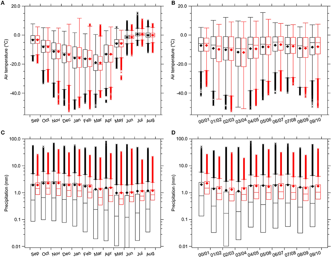
Figure 4. Comparison of the distributions of air temperature (A,B) and precipitation (C,D) in the WRF dataset (black) and the downscaled ERA-20C dataset (red). For both climate variables, intra-annual (A,C) and inter-annual variability (B,D) are shown. The box plots are based on data from the mass-balance years 2000/2001–2009/2010 and include values from all glacier relevant grid points across the Svalbard archipelago (cf. Figure 1). Means are indicated by filled diamonds, and outliers as individual symbols beyond the whisker ranges.

Climate data across Kvitøya we consider with special care because of the erroneous WRF elevations in this area (cf. section Overall Basics). The far too flat terrain presumably affected the reliability of the WRF precipitation and air temperature data used as reference during the first step of downscaling. We assume WRF precipitation across the island to be too low due to missing orographic uplift and WRF air temperatures to be too high. Hence, we also assume the interpolated precipitation of the final 250 m domain as too low. Air temperatures of the final 250 m domain are less affected as the applied lapse rates imply an adjustment to the reliable 250 m topography. However, even for air temperatures negative effects on their accuracy across Kvitøya cannot be ruled out completely due to the usage of archipelago-wide mean lapse rates instead of local lapse rates during the second step of downscaling. As a result of this, we do not explicitly report on mass balances of Kvitøya (subregion 9), but rather include data from this subregion only in archipelago-wide integrations.

Mass-Balance Modeling

Model Description

To calculate CMB, accumulation, ablation and refreezing at each single day are summed up. Hereby, ablation is included as a negative quantity. Differentiation of the archipelago-wide CMB fields into subregions (cf. Figure 1) is done across the grid points of the 10 km intermediate domain. Afterwards, an integration over the respective associated grid points yields the subregion- or archipelago-wide CMB.

Accumulation is assumed to be equal to the solid portion of precipitation. Discrimination between liquid and solid precipitation is done according to a hyperbolic function (Möller et al., 2007). The solid portion of precipitation (P_s) is calculated depending on air temperature (T) and ranges between 100% (−1°C) and 0% (+3°C) of total precipitation (P):

\begin{array}{l} P_{s} = 0.5 \cdot P \cdot (-tanh [1.1 \cdot (T - 1.0)] + 1.0) & (5) \end{array}

The threshold air temperatures for full attribution to either solid or liquid precipitation are chosen to resemble characteristic conditions on Svalbard as described by Førland and Hanssen-Bauer (2003).

Ablation is calculated from positive air temperatures by applying degree-day factors of 11.2 mm w.e. K⁻¹ d⁻¹ for snow surfaces and 14.1 mm w.e. K⁻¹ d⁻¹ for ice surfaces. These factors have been calibrated using in situ mass balance measurements (cf. section Calibration). To discriminate between the two surface types a bookkeeping of snow depth is done over the modeling period.

Refreezing is calculated from model meltwater and rain, which are assumed to completely refreeze inside the snowpack until a predefined amount is reached. This maximum amount of refreezing (R_max) is updated on an annual basis and is calculated following Wright et al. (2007):

\begin{array}{l} R_{m a x} = \frac{c_{i c e} \cdot d}{2.0 \cdot L_{f}} \cdot [(1.0 - \frac{π}{2.0}) \cdot \bar{T_{a}} - \bar{T_{w}}] & (6) \end{array}

In Equation (6), c_ice is the specific heat capacity of ice (2,097 J kg⁻¹ °C⁻¹), d is the assumed penetration depth of the annual temperature cycle (5.0 m), L_f is the latent heat of fusion of ice (3.334 10⁵ J kg⁻¹), $\bar{T_{a}}$ is the mean annual and $\bar{T_{w}}$ the mean winter air temperature. As soon as R_max is reached in the course of an ablation season, any excess meltwater or rain turns directly into runoff.

Calibration

The mass balance model is calibrated to fit regional conditions on Svalbard by adjusting the degree-day factors for snow and ice and by scaling the precipitation amounts. The in situ reference for adjustments and scaling is given by 160 seasonal mass balance measurements at ten mass balance stakes on Kongsvegen glacier (Figure 1). The stakes are installed across the elevation interval 160–720 m a.s.l.; seasonal measurements are from the period 2000–2008.

During the calibration procedure the three tuning parameters are varied simultaneously within reasonable ranges until the root mean square (RMS) error between modeled and measured CMB is minimized. For degree-day factors of 11.2 mm w.e. K⁻¹ d⁻¹ for snow surfaces and 14.1 mm w.e. K⁻¹ d⁻¹ for ice surfaces and a precipitation scaling factor of 1.2 the RMS error reaches its global minimum (0.54 m w.e.). For this combination of parameters modeled CMB shows no systematic bias compared to measured values; R² is 0.70.

For Svalbard a considerable variability of degree-day factors for snow has been documented. Killingtveit and Sælthun (1995) reported on a range of 3.0 to 6.0 mm K⁻¹ d⁻¹ while Bruland et al. (2001) give a value of 7.0 mm K⁻¹ day⁻¹. Degree-day factors which are assumed for Svalbard glaciers in global modeling studies also resemble this magnitude [e.g., 7.2 mm K⁻¹ day⁻¹; Radić and Hock (2011)]. However, Sand (1990) even describes snow melt rates between 0.0 and 6.0 mm h⁻¹ measured within a period not warmer than +6°C. Assuming that the highest melt rates occurred at the highest air temperatures this would yield a maximum degree-day factor of 24 mm K⁻¹ day⁻¹. Hence, our calibration result of 11.2 mm w.e. K⁻¹ d⁻¹ for snow surfaces is reasonable.

Studies presenting Svalbard-specific degree-day factors for ice are less numerous. In the global modeling study of Radić and Hock (2011) a value of 9.0 mm K⁻¹ day⁻¹ is assumed. In contrast, Schytt (1964) reported a degree-day factor for ice of 13.8 mm K⁻¹ day⁻¹ which was measured on Vestfonna. Hence, our calibration result of 14.1 mm K⁻¹ day⁻¹ for ice surfaces is indeed rather high but still reasonable.

Validation

Modeled CMB is validated against point mass balance data based on firn coring results presented in two earlier studies (Table 2). Pinglot et al. (1999) report mean mass balances over periods of 5 to 33 years for 10 different locations on glaciers in subregions 1, 3, 6, and 7 (Figure 1). Beaudon et al. (2011) report additional mean mass balances from a firn coring site in subregion 6. For each of the eleven validation locations, the core-based mean mass balances are compared to corresponding mean modeled CMB. Modeled CMB is also compared to glacier-wide CMB available for four glaciers from in situ measurements or glacier-specific modeling (Figure 5). Measured balances are available since the late 1960s for the small valley glaciers Austre Brøggerbreen and Midtre Lovénbreen, as well as since the mid 1980s for the larger valley glacier Kongsvegen, all three of them are located close to the western coast of Spitsbergen. Modeled CMB for a three-decade period, supported by extensive field data, are available for the large ice cap Vestfonna (Möller et al., 2013).

TABLE 2

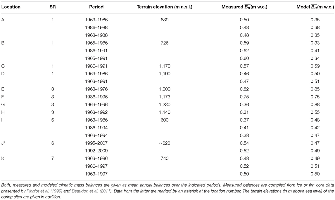
Table 2. Comparison between modeled and measured climatic mass balance (in m water equivalent) at eleven different locations (cf. Figure 1).

FIGURE 5

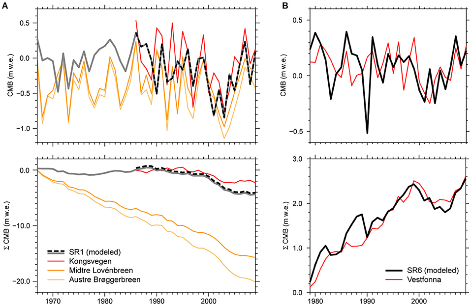
Figure 5. Multi-decadal comparison of modeled subregion-wide climatic mass balances to glacier-wide balances of Kongsvegen, Austre Brøggerbreen and Midtre Lovénbreen (A) which are derived from regular in situ measurements, and to ice cap-wide balances of Vestfonna (B) which are obtained from more sophisticated modeling (Möller et al., 2013). Upper panels show annual balances, while lower panels give the cumulative view. Note that measured balances for Kongsvegen have a later start date, leading to a differing cumulative balance over the respective shorter measurement period (dashed line).

The point mass balance comparison reveals no systematic bias between modeled CMB and in situ measurements (Table 2); the mean discrepancy is just −0.004 ± 0.17 m w.e. (mean ± one sigma). However, the relatively large standard deviation (0.17 m w.e.) of the CMB discrepancies and the root mean square (RMS) error of ±0.16 m w.e. between measured and modeled CMB suggest considerable variability between the different locations.

The by far largest discrepancy (+0.52 m w.e.) is found at the most high-lying coring location G in subregion 3 (Table 2). Measured balances amounts to +0.36 m w.e., while model CMB is distinctly higher at +0.88 m w.e. Comparably high overestimations also occur in the recent 1957–2014 modeling study of Østby et al. (2017). Moreover, a snow-radar study presented in Pälli et al. (2002) shows highly variable snow accumulation rates along an altitudinal profile in the area of three of the respective coring locations. Over a distance of ~11.5 km measured annual accumulation rates roughly vary between 0.4 and 1.0 m w.e. a⁻¹, with changes from one extreme to the other repeatedly occurring over sub-kilometer distances. This suggests that the high estimates might partly be a result of coring locations situated at locally limited low-accumulation sites. This interpretation is also supported by the fact that coring location G is situated on a wind-exposed hilltop where accumulation can be assumed to be substantially reduced by snow drift losses.

The comparison of glacier-wide mass balances reveals a good reproduction of inter-annual variability at all four reference glaciers (Figure 5). With few exceptions, periods of more or less negative balance years are matched and the timing of singular peaks in one or the other direction is met quite often. For the ice cap Vestfonna, i.e., subregion 6 in this study, also the cumulative balance over 32 years which has been reliably calculated by Möller et al. (2013) using a spatially distributed temperature-net shortwave radiation index model in combination with site-specific albedo modeling is reproduced almost perfectly. However, it has to be borne in mind that a comparison with the results of a previous modeling study can only indicate similarity but not necessarily provides evidence of accuracy. Also the measured cumulative balance of the valley glacier Kongsvegen, located in subregion 1, is reproduced almost perfectly by the cumulative balance of the subregion modeled in this study. For the two valley glaciers Austre Brøggerbreen and Midtre Lovénbreen, which are also located in subregion 1, measured cumulative balances are, in contrast, by far smaller than the modeled subregion-wide cumulative balance. However, this is in large part explainable by the scale and hypsometry differences between the small valley glaciers with their rather limited accumulation areas and the extensive ice fields, forming most of subregion 1, with their large and high-lying accumulation areas. The latter implies distinctly less negative balances. Taken together, the comparisons to independent mass balance data or studies support the CMB modeled in this study to a very reasonable degree.

Model Sensitivity

The sensitivity of modeled CMB is assessed for the two model input variables and three model parameters (Figure 6). We test the sensitivity of the CMB model to perturbations or deviations of these quantities rather than performing a detailed uncertainty assessment, as the latter would require reliable uncertainty estimates for each of those quantities, which cannot be derived though.

FIGURE 6

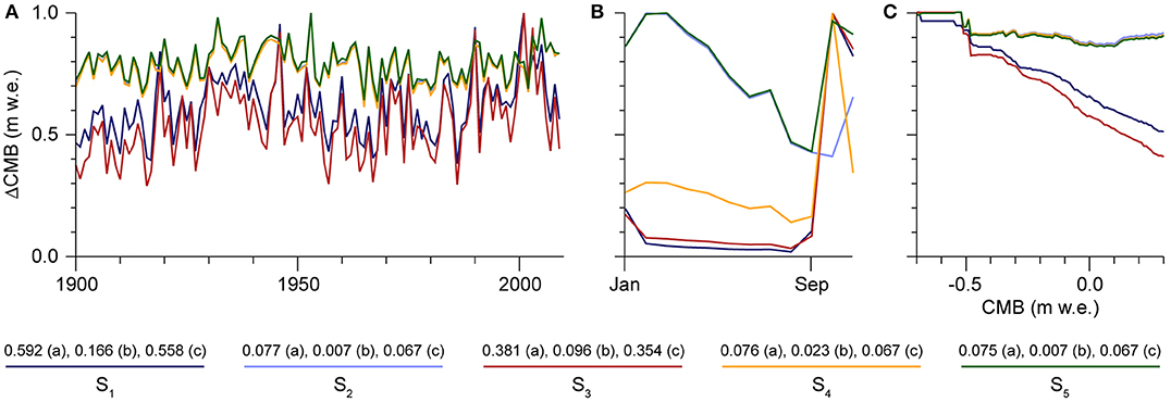
Figure 6. Sensitivities of the modeled climatic mass balances to perturbations in model input variables and model parameters. Sensitivities are given as annual values over 1900–2010 (A), as monthly values in mean inter-annual courses (B) and in relation to annual climatic mass balance itself (C). The numbers are normalized by dividing by the respective maximum value of the dataset. All maximum values are given in the figure legend. The different sensitivities S₁ to S₅ are described in section Model Sensitivity.

The sensitivities of the model to perturbations in air temperature and precipitation inputs (S₁ and S₂) are assessed by performing additional model runs either with air temperatures shifted by ±1.0°C or with precipitation scaled by ±10%.

The sensitivities of the model to deviations in the selected degree-day factors in the ablation calculation for snow and for ice (S₃) are quantified by altering these factors within a range of ±20%. Hence, additional model runs are performed using degree-day factors of 14.1 ± 2.8 mm w.e. K⁻¹d⁻¹ for ice surfaces and 11.2 ± 2.2 mm w.e. K⁻¹d⁻¹ for snow surfaces.

The sensitivity of the model to deviations in the assumed penetration depth of the annual air temperature cycle (S₄) into the glacier, which is relevant during refreezing calculation (cf. Equation 6) is quantified by altering the depth within a range of ±20%. The related additional model runs are performed using penetration depths of 5.0 ± 0.5 m.

The sensitivity of the model to deviations in the selected transition range between solid and liquid precipitation (S₅), which is realized between −1.0 and +3.0°C according to detailed in situ data reported by Førland and Hanssen-Bauer (2003), is quantified by shifting the centre of this range (+1.0°C) by ±0.5°C. The additional model runs are thus performed with transition ranges either between −1.5 and +2.5°C or between −0.5 and +3.5°C.

Model sensitivities cluster in two different groups in several respects. First is magnitude (Figure 6A), where S₁ and S₃ are one order larger than S₂, S₄ and S₅. Second is evolution over the study period (Figure 6A), where S₁ and S₃ differ markedly from S₂, S₄ and S₅ in their inter-annual course and show a significantly positive (95% level) trend over time which S₂, S₄ and S₅ do not. Third is the mean intra-annual course (Figure 6B), where S₂ and S₅ dominate over the accumulation season while S₁, S₃ and S₄ do so over the ablation season. Fourth is the pattern of the dependency on annual CMB (Figure 6C), where S₁ and S₃ decrease markedly with increasing CMB while S₂, S₄ and S₅ do not. As the groupings in second and fourth match perfectly, it can be assumed that the significant trend in S₁ and S₃ over time is a result of decreasing annual CMB over the study period and not a model feature.

Results

The CMB across all glacierized areas of the Svalbard archipelago over the period 1900–2010 is quasi balanced at −0.002 ± 0.24 m w.e. a⁻¹ with an associated equilibrium line altitude (ELA) of 425 m a.s.l. (Table 3; Figure 7). This is because the mass gains during the winter seasons of the study period show a mean rate of +0.49 ± 0.11 m w.e. a⁻¹ and thus compensate for the concurrent mass losses during the summer seasons, which have a mean of −0.49 ± 0.20 m w.e. a⁻¹ (Table 3).

TABLE 3

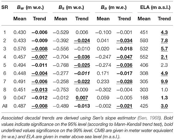
Table 3. Mean winter (B_w), summer (B_s) and annual (B_a) glacier-wide climatic mass balances (CMB) and equilibrium line altitudes (ELA) for all Svalbard and its nine different subregions (cf. Figure 1) over the mass-balance years 1900/1901–2009/2010.

FIGURE 7

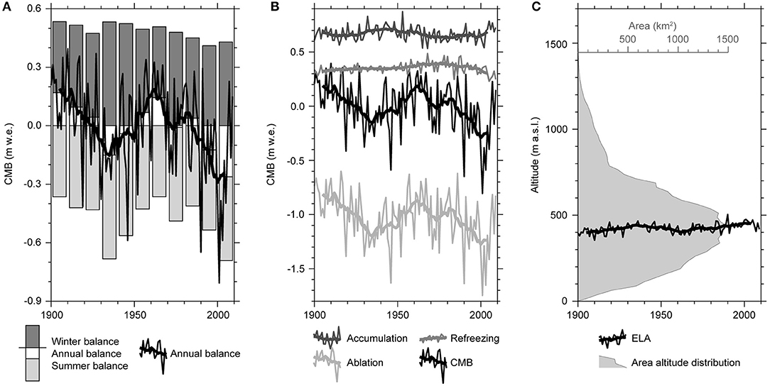
Figure 7. Modeled archipelago-wide climatic mass balances (CMB) and equilibrium line altitudes (ELA) over the mass-balance years 1900/1901–2009/2010. (A) Mean decadal winter, summer and annual balances are given as bar chart, the annual balances (thin line) together with a running decadal mean (thick line) as line graph. (B) Annual CMB components (thin lines) are shown together with running decadal means (thick lines). (C) Annual ELAs (thin line) and the running decadal means (thick line) are shown together with the area altitude distribution (gray shading) of all glacierized areas of Svalbard. The area altitude distribution is calculated in 25 m bins.

This general picture shows substantial variability over time, with some cyclicity (Figure 7A). Decreasing balances characterize the first four decades of the twentieth century, followed by increasing ones until the early 1960s. Afterwards, the cycles become shorter. Balances decrease until the early 1970s and increase again until the early 1980s. Finally, a decrease of balances until around 2000 is replaced by an increase over the first decade of the twenty-first century. This temporal pattern is clearly induced by ablation variability which shows similar cyclicity as CMB (Figure 7B). Accumulation and refreezing remain rather constant in comparison, but nevertheless show characteristic pattern even though at lower amplitudes (Figure 7B). Accumulation seems to follow an ~60 years cycle with lowest values in the 1910s and 1970s and highest values in the 1930s. Refreezing increases continuously until the 1970s and afterwards decreases likewise continuously (even though at higher rates) to values below those at the begin of the study period. It contributes 34% to the archipelago wide mass gain on average (Figure 8). Across the individual subregions this contribution ranges between 29% (subregion 5) and 39% (subregion 6).

FIGURE 8

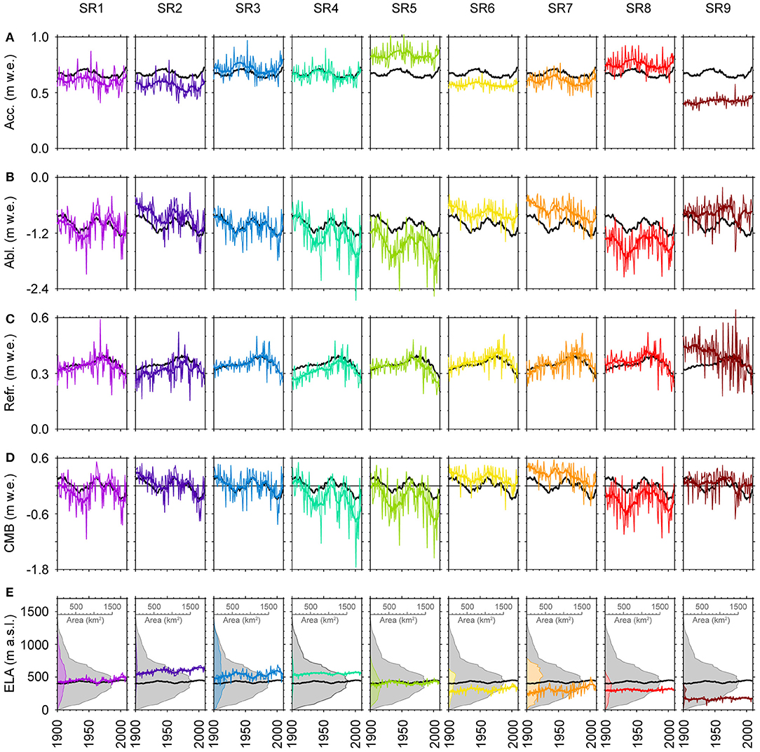
Figure 8. Annual climatic mass balance (CMB) components and equilibrium line altitudes (ELA) for the nine different subregions (cf. Figure 1; Table 1) over the mass-balance years 1900/1901–2009/2010: (A) accumulation, (B) ablation, (C) refreezing, (D) CMB, (E) ELA. Annual values (thin color-coded lines) are given along with running decadal means (thick color-coded lines). The archipelago-wide running decadal means (thick black lines) are shown for comparison. The ELAs are shown together with the area altitude distribution (color-coded shading) of the glacierized area in the respective subregion. The area altitude distribution of all glacierized areas of Svalbard (gray shading) is shown for comparison. All area altitude distributions are calculated in 25 m bins.

The cyclicity of CMB is superimposed over a highly significant (99% level according to Mann-Kendall trend test) trend of −0.021 m w.e. per decade over the study period (Table 3), providing evidence for a development toward a more negative archipelago-wide CMB. The latter is induced by both, a highly significant (99% level) decrease of winter balances along a trend of −0.008 m w.e. per decade and a significant (95% level) decrease of summer balances along a trend of −0.013 m w.e. per decade. Accordingly, positive balances clearly prevail during ~1900–1980, while toward the end of the twentieth century negative balances become more frequent. Fitting to this pattern, also the ELA shows a highly significant (99% level) trend of +3.0 m a.s.l. per decade over the study period (Table 3; Figure 7C).

A marked exception from this pattern is evident in the 1930s. Annual balances are negative over the entire decade except for 1932/1933 (Figure 7A). From 1933/1934 until the early 1940s nine consecutive mass balance years show negative archipelago-wide balances. This is unprecedented over the entire 110 years study period. This exceptional situation in the 1930s can be ascribed to the highest ablation sums in all of the twentieth century; only in 2000–2010 was ablation more pronounced (Figure 7B). Accordingly, the 1930s are the most negative decade in the twentieth century (−0.15 m w.e.), even exceeding the 1990s (−0.12 m w.e.). This is in spite of winter balances being distinctly more positive in the 1930s than in the 1990s (Figure 7A), a fact that highlights the exceptional strength of the ablation seasons in the 1930s. Both decades are, however, clearly exceeded by the first decade of the 21st century, which shows the most negative balance in the overall study period (−0.26 m w.e.).

Year 2001/2002 appears to be the most negative mass balance year (−0.81 m w.e.), followed by 1990/1991 (−0.65 m w.e.) and 1946/1947 or 2003/2004 (−0.59 m w.e.; Figure 7A). Conversely, 1910/1911 is the most positive mass balance year (+0.39 m w.e.), followed by 1927/1928 (+0.37 m w.e.) and 1917/1918 (+0.36 m w.e.).

In addition to the temporal variability of CMB, substantial spatial variability is evident. While the northeastern parts of the archipelago show predominantly positive CMB, the western and southern parts are characterized by rather negative balances (Figure 8D; Table 3). The ELAs are lowest in the eastern parts (subregions 8, 7, and 6) and highest in the central parts of the archipelago (subregions 2, 4, and 3; Figure 8E). This latitudinal and zonal variability is overlain by an elevational variability. Glacierized areas on higher terrains show more positive balances than glaciers on lower terrains (Figure 9). Throughout the highest (subregions 1 and 3) and most interior (subregions 6 and 7) parts of the archipelago even the summer balances show distinctly positive means over the 110 years of the study period. Hence, the more high-lying subregions on Spitsbergen show positive mean balances over the study period while the more low-lying show negative ones (Figure 8; Table 3). All subregions show statistically significant, negative winter balance trends and thus mirror the overall, archipelago-wide development (Table 3; Figure 9A). The picture is variable when it comes to summer balances (Table 3); in five out of nine subregions significantly negative trends are evident, indicating a development toward more strongly negative ablation seasons. However, in three subregions tendencies toward less negative summer balances were found. The fact that these subregions do not show significantly positive overall trends is caused by a spatial limitation of the positive trends to certain parts of the respective subregions (Figure 9B). Extensive coherent areas with significantly positive trends are observable in the interior of subregion 1 north of Isfjorden (1,839 km², showing a mean trend of +0.086 m w.e. per decade) and across the eastern part of Edgeøya in subregion 8 (1,270 km², showing a mean trend of +0.035 m w.e. per decade). Overall, the limited spatial extent of these areas with positive summer balances still allows for a significantly negative trend in archipelago-wide summer balances (Table 3).

FIGURE 9

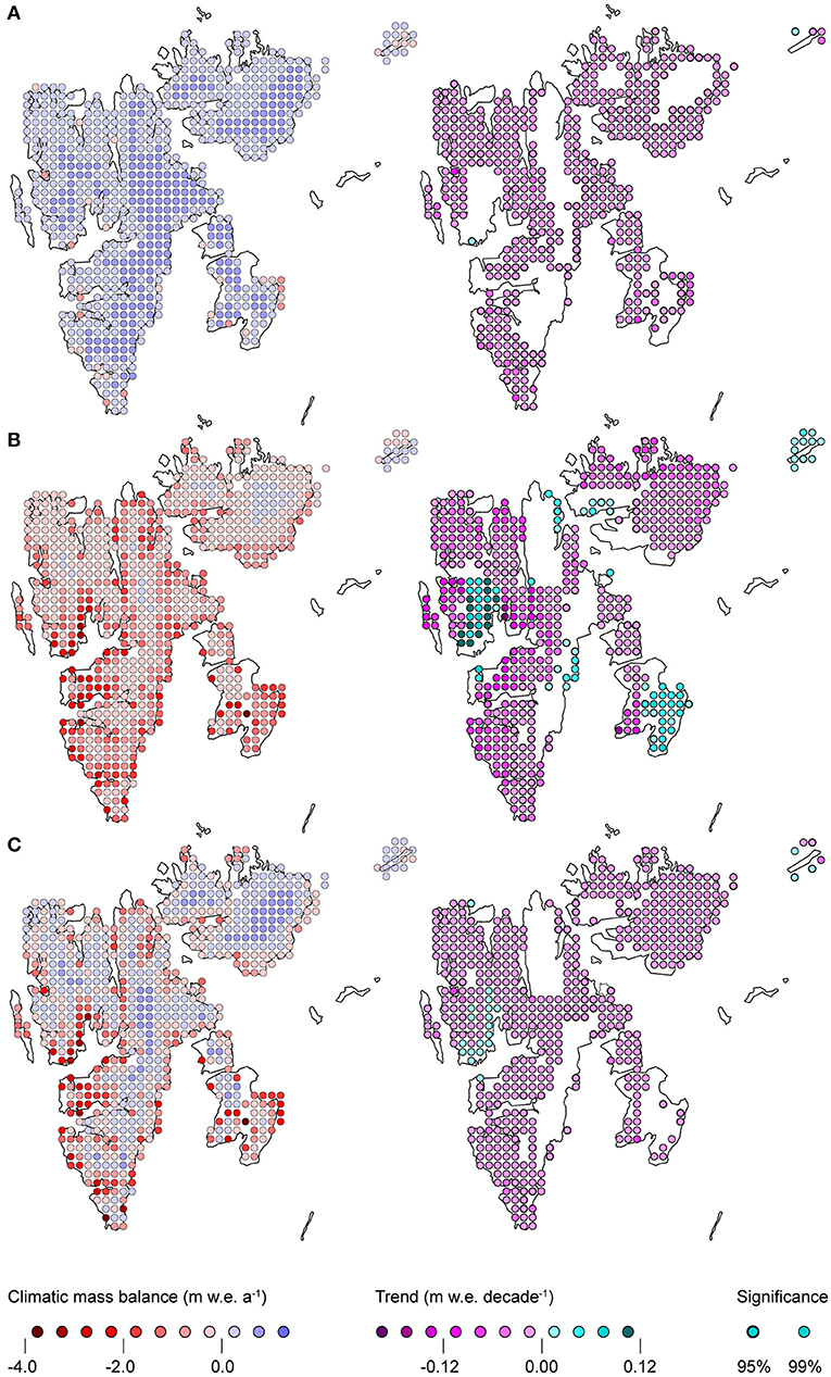
Figure 9. Mean modeled climatic mass balance fields for Svalbard over the mass-balance years 1900/1901–2009/2010 and associated decadal trends. (A) Mean winter balance is shown together with (B) mean summer balance and (C) mean annual balance. The three trend fields only show grid points for which the climatic mass balance trend has a statistical significance of at least 95% according to the Mann-Kendall trend test. The slopes of the trends are derived using Sen's slope estimator (Sen, 1968).

Austfonna (subregion 7) shows by far the most positive subregion-wide balances in all over Svalbard (Figure 8). Exclusively, this holds true only until the mid 1960s. From then on Vestfonna (subregion 6) shows an equally positive state of CMB. The mean annual balance of subregion 7 amounts to +0.23 ± 0.21 m w.e.; the associated ELA is 305 ± 71 m a.s.l. (Table 3). This situation of exceptionally positive balances is due to the lowest ablation on the archipelago (Figure 8B; Table 3). It leads to very low ELAs which, in combination with the distinctly top-heavy area altitude distributions, leads to strongly positive balances even though subregion 7 is characterized by rather low accumulation sums (Figure 8). As typical for the entire archipelago Austfonna shows a highly significant trend toward less positive annual balances (−0.028 m w.e. per decade). Despite showing the least negative 110 year mean summer balance of all subregions, subregion 7 also shows a highly significant, strongly negative trend in summer balance (−0.022 m w.e. per decade), which is equal to that in the high-ablation subregion 5.

The subregion with the most negative CMB cannot be identified as clearly (Figure 8; Table 3). Subregion 8 in fact shows the most negative mean annual balance over the 110 years study period (−0.30 ± 0.32 m w.e. a⁻¹) but with a high variance over individual years and without any significant trend. Subregions 5 and 4, in contrast, are only slightly less negative (−0.27 ± 0.39 m w.e. a⁻¹ and −0.25 ± 0.39 m w.e. a⁻¹) but show even higher variances (Figure 8D) and significant trends toward even more negative annual balances (Table 3). Correspondingly, subregion 8 is the most negative only over the first four decades of the study period. From the mid 1980s onwards, subregions 4 and 5 take over at similar annual rates (Figure 8D). In between, no clear ranking between the three subregions is possible. Overall, the distinctly negative balances in these three subregions are a result of the by far highest ablation sums (Figure 8B) and most strongly negative summer balances across the archipelago (Table 3). Accumulation sums have no influence here; subregions 5 and 8 even feature the by far highest accumulation across the archipelago (Figure 8A). Subregion 8 even shows the lowest mean ELA of all subregions (303 m a.s.l.) that does, moreover and in contrast to the rest of the archipelago, not show any significant trend toward higher elevations (Table 3). The seeming contradiction between most negative balance and lowest ELA in subregion 8 can, however, be explained by the fact that the large and contiguous ice bodies of this subregion are limited to distinctly lower elevations than it is the case for the rest of the archipelago (Table 1; Figure 8E).

A striking difference in temporal CMB evolution is evident across the three subregions (1, 2, and 3) covering the northern half of Spitsbergen. The annual balance of subregion 3 develops along the archipelago-wide average despite a distinctly above-average accumulation (Figure 8). Subregions 1 and 2, in contrast, show opposed evolutions in this respect. Over the second half of the study period both of them develop along the archipelago-wide average as also subregion 3 does. However, over the first half, subregion 1 shows distinctly more negative but subregion 2 distinctly more positive annual balances (Figure 8D). This pattern is induced by distinct differences in the trends in ablation and summer balance. While subregion 1 does not show any significant trends in this respect, a significant trend toward more negative summer balances is evident across subregion 2 (Table 3).

Discussion

Our archipelago-wide CMB values are widely in accordance with those obtained in previous studies. However, on a subregional scale, noticeable differences appear. The temporal variability of the CMB values mirrors the overall warming trend observed over the twentieth century and also the early twentieth century Arctic warming episode is clearly identifiable in the modeled CMB time series.

Three modeled CMB time series have been presented for Svalbard so far and their results are similar to ours. In the longest term, Østby et al. (2017) obtained a mean annual CMB of +0.08 m w.e. for entire Svalbard over 1957–2014. Our results show a value of −0.03 m w.e. over 1957–2010. Lang et al. (2015) obtained a mean annual CMB of −0.05 m w.e. for Svalbard excluding Kvitøya (subregion 9) over the period 1979–2013, while our modeling yields a similar value of −0.11 m w.e. over the slightly shorter period 1979–2010. A comparison to the results of the sophisticated modeling study of Aas et al. (2016), who calculated the CMB of Svalbard (excluding Kvitøya) for 2003–2013, also reveals similar results. Over the period 2003–2008 our study yields −0.21 m w.e. while Aas et al. (2016) obtained −0.18 m w.e.

This consistency is further supported by satellite-based observations, i.e., gravity measurements and laser altimetry. Interpretations of GRACE (Gravity Recovery and Climate Experiment) data over Svalbard revealed ice mass losses equivalent to mass balance values between −0.09 ± 0.05 for 2003–2010 (Jacob et al., 2012) and −0.27 ± 0.12 to −0.46 ± 0.07 m w.e. for 2003–2009 (Mémin et al., 2011). Our CMB modeling yields −0.15 and −0.19 m w.e., respectively, over these periods. Given the observed mean annual ice mass loss of −0.20 m w.e. across Svalbard due to calving fluxes and calving front retreats (Błaszczyk et al., 2009), which are not included in our CMB values, the two different types of mass balance estimates match each other. A comparison to laser altimetry derived geodetic mass balances in recent years, however, reveals a contrasting picture. Moholdt et al. (2010b) found a mean annual value of −0.12 ± 0.04 m w.e. over all Svalbard in 2003–2008, neglecting effects of calving front retreats. This yields a mass balance equivalent of +0.02 m w.e., when considering the mean annual calving flux (but excluding calving front retreats), estimated to be −0.14 m w.e. over recent years (Błaszczyk et al., 2009). Our modeled mean annual CMB over this period is more negative at −0.20 m w.e.

When looking at individual subregions over longer time scales the comparison to observed geodetic balances partly improves. From the mid 1960s until 2005 northwest Spitsbergen (subregions 1 and 2) and northeast Spitsbergen (subregion 3) showed distinctly negative balances of −0.41 and −0.25 m w.e. (Nuth et al., 2010). Our modeled CMB for this period (−0.09 and −0.05 m w.e.) shows only slight overestimations as soon as mass losses from calving fluxes and calving front retreats are taken into account, both of which are included in the geodetic balances of Nuth et al. (2010). For central and southern Spitsbergen (subregions 4 and 5) and for Barentsøya and Edgeøya (subregion 8) the balances derived by Nuth et al. (2010) for the period 1990–2005 (−0.55 and −0.50 m w.e.) are more positive than our modeled balances (−0.64 and −0.48 m w.e.), when calving fluxes and calving front retreats are taken into account. For Vestfonna (subregion 6) our modeling yields a mean annual CMB of +0.01 m w.e. during 1990–2005, while Nuth et al. (2010) derived a mean annual geodetic balance of +0.05 m w.e., including mass losses due to calving fluxes and calving front retreats. This suggests an underestimation of CMB by our model in subregion 6. Over a shorter time period (2003–2008) the subregional picture becomes even more diverse (Table 4). Comparing our study to the observed geodetic balances of Moholdt et al. (2010b) reveals overestimations across northwestern Spitsbergen (subregions 1 and 2), matching estimates on Vestfonna (subregion 6) and underestimations across northestern, central and southern Spitsbergen (subregions 3, 4, and 5), on Austfonna (subregion 7) and across Barentsøya and Edgeøya (subregion 8).

TABLE 4

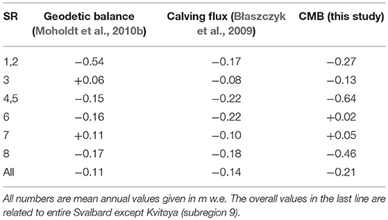
Table 4. Comparison of our modeled climatic mass balances to observed geodetic balances for different parts of Svalbard over the period 2003–2008.

Taken together, the comparisons with the different observational and modeling studies reveal a spatially continuous pattern. Our model overestimates the CMB across the northwestern parts of Spitsbergen (subregions 1 and 2). It underestimates the CMB across southern Spitsbergen (subregions 4 and 5), Austfonna (subregion 7) and Barentsøya and Edgeøya (subregion 8). An uncertain relation of our modeling results to observed balances is evident across northeast Spitsbergen and Vestfonna (subregions 3 and 6). This suggests a NW-SE gradient from too high to too low CMB for our model results.

The coincidence of this pattern with the elevation distribution across the different subregions (Table 1; Figure 8E) suggests a generally too large mass balance gradient. Across the more high-lying subregions of Svalbard this would imply excess accumulation while across the more low-lying subregions excess ablation would be the result. For subregion 3, which holds both, extensive high-lying and low-lying glacierized areas (Figure 8E), the picture is unclear. When interpreting this spatial pattern of over- and underestimations further, it has to be borne in mind that all geodetic balances considered as observation-based references are also too negative as they not account for any mass conservation by refreezing processes, which happen independently of surface elevation changes. However, since refreezing processes contribute substantially to the CMB of Svalbard glaciers (e.g., Wright et al., 2007; Østby et al., 2013; Möller and Schneider, 2015), it is reasonable to assume that the overestimation of CMB might actually be smaller than inferred here, but that the underestimation, in turn, is even larger. However, a quantification of this effect is not possible.

A generally striking feature of the modeled archipelago-wide CMB time series is the temporary negative record of CMB during the 1930s (Figure 8D), which coincides with the peak of the early twentieth century Arctic warming. As such a pattern has also been modeled for the mass balance of the Greenland ice sheet (Fettweis et al., 2017), it is reasonable to assume that the drop in CMB on Svalbard over these years is not an isolated, regional pattern, but reflects an overall Arctic warming episode. Nevertheless, the development toward negative CMB varies substantially across the archipelago. In the north half of the archipelago (subregions 1, 2, 3, 6, and 7) the drop toward the temporal CMB minimum already starts in the early 1900s. In the northeastern parts (subregions 3, 6, and 7) the minimum is reached in the mid 1930s, while in the northwestern parts (subergions 1 and 2) the development is slower and the temporal CMB minimum is not reached until the late 1930s. In the southern half of the archipelago (subregions 4, 5, and 8) the temporal CMB minimum is already reached in the early 1930s, but the drop toward these values does not start before the early 1910s (Figure 8D).

The bottom line of this pattern of temporal differences matches in parts with the pattern of over and underestimations described earlier. Across northwestern Spitsbergen CMB was suggested to be overestimated due to excess accumulation induced by a too large CMB gradient. This excess accumulation in the model might have initially buffered the drop of CMB toward its temporal minimum during the early twentieth century Arctic warming episode, leading to a later culmination. The one-decade difference between northern and southern half of Svalbard regarding the onset of the development toward negative CMB, however, cannot be explained by model features.

Our modeling results suggest statistically significant negative trends of CMB across most of Svalbard in combination with mostly significant positive trends in ELA (Figures 7, 8; Table 3). This is exactly what one would expect when looking at a recent, century-long CMB time series for an Arctic region, as the influences of climate warming have been most pronounced across the northernmost parts of the globe. Also a recent study of glacier surface albedo variability, which is clearly related to ELA differences, revealed significantly negative trends in albedo across Svalbard (Möller and Möller, 2017), indicating a rising ELA. However, two regions stick out from this overall pattern; the eastern part of Edgeøya (in subregion 8) and the southern part of subregion 1. The significantly positive summer balance trends in these regions are not explainable by any climate-related reasons.

One possible explanation would be a topography-related feedback in a way that ongoing glacier retreat over the century eliminated large parts of a low-lying ablation area, leaving the respective glacier mainly with a high-lying accumulation area, thus leading to distinctly more positive, glacier-wide CMB values after the loss of the ablation area, and with it to a positive CMB trend. However, this possibility has to be discarded, as our model calculates reference-surface balances, i.e., balances that, unlike conventional balances, are based on a fixed surface topography and a fixed glacier extent. This fact, in turn, introduces a likely, alternative and method-inherent explanation.

Schäfer et al. (2015) showed that reference-surface balances distinctly overestimate the conventional balance in century-long CMB calculations toward the end of the run due to missing consideration of lateral mass loss and surface lowering. This implies a less negative trend in the reference-surface balance than in the conventional balance. This feature is equally present no matter if CMB is calculated on the basis of glacier topography and extent from the beginning or the end of the modeling period.

The large ice field on Edgeøya showed the largest retreat rates of all Svalbard glaciers over the last decades (Nuth et al., 2013). Hence, it is likely that the positive trend of CMB on Edgeøya is not characteristic of this area, but merely a result of the increasing underestimation of the real (conventional) CMB compared to the modeled (reference-surface) CMB, when going back toward the beginning of the twentieth century. The same could also hold for the area of positive reference-surface CMB trends in the southern part of subregion 1. This area is part of the major drainage basin showing the second largest area losses on Svalbard after Edgeøya (Nuth et al., 2013). Indeed, one could argue that a similar effect should appear across the entire archipelago, as glaciers are retreating everywhere in Svalbard (Nuth et al., 2013). However, retreat rates across the rest of Svalbard are smaller than those observed on Edgeøya and around Isfjorden (Nuth et al., 2013) and the above described effect might thus be not as pronounced, leaving the signs of the CMB trends untouched. Notwithstanding this reasonable explanation, it cannot be ruled out that the regionally limited features of significantly positive CMB trends are also an indirect expression of general modeling uncertainty.

When looking at our modeled CMB as cumulative values over the entire 110 years modeling period (Figure 10), the four northeastern-most subregions (2, 3, 6, and 7) emerge as net-positive, while the four western and southern most subregions (1, 4, 5, and 8) as net-negative. However, this picture is misleading in terms of the overall mass balance. Additional mass loss due to calving fluxes makes up for a huge total over the twentieth century. When adding the mean annual calving flux estimates of Błaszczyk et al. (2009) for each of the subregions the pattern of positive and negative areas on the archipelago changes considerably (Figure 10C). Only subregions 2 and 7, out of which the former has no tidewater glaciers and thus no calving losses, remain in the net-positive area. For all other subregions the cumulative mass balance over 1900–2010 is negative. This also tears the archipelago-wide average into the net-negative sector. After the 110 years of our modeling period the overall mass balance of entire Svalbard is −16.9 m w.e., which equals a sea level rise contribution of ~1.6 mm when assuming the total ocean area of Cogley (2012) (362.5 Mm²).

FIGURE 10

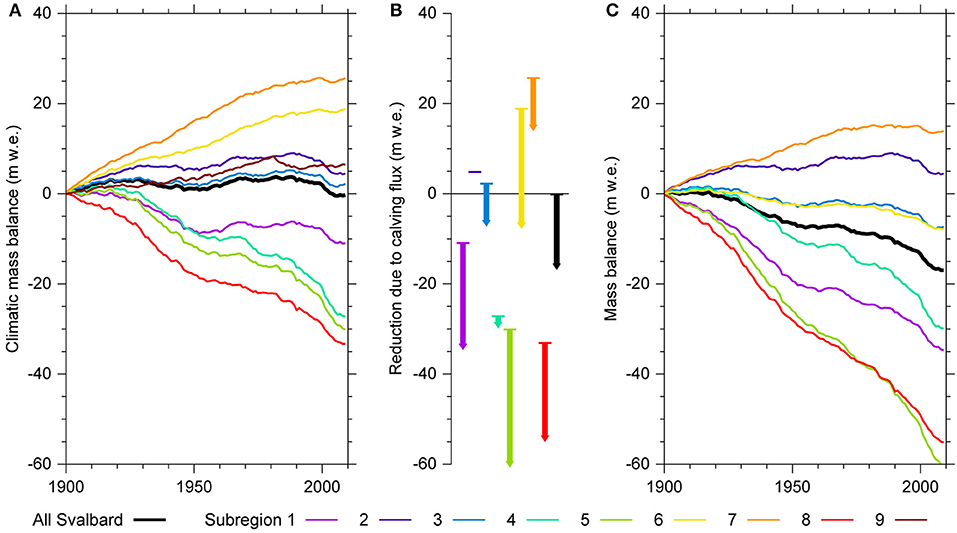
Figure 10. Cumulative mass balance evolution for Svalbard and its nine different subregions over the mass-balance years 1900/1901–2009/2010: (A) Climatic mass balance (CMB), (B) reduction due to calving flux, (C) Mass balance, i.e., CMB with calving flux added. The calving fluxes are given as bar charts representing 110-years totals according to mean annual values presented by Błaszczyk et al. (2009). Individual bars start with the thin horizontal line at the level of the final cumulative CMB of the respective subregion (cf. panel A) and end at the level of the respective final cumulative mass balance (cf. panel C). For creation of the cumulative mass balance time series in panel (C) constant annual calving fluxes are added to the cumulative CMB shown in panel (A). Note that no tidewater glaciers exist in subregion 2. As no information on calving is available for subregion 9 it is not included in panel (C).

Conclusion

The climatic mass balance of all glacierized areas across the Arctic archipelago Svalbard was modeled for the period 1900–2010. Daily calculations were done on a regular 10 km grid using a degree day method-based model. Model forcing was provided by statistically downscaled ERA-20C reanalysis data. Results were analyzed as archipelago-wide means and subdivided into nine different subregions.

Results indicate an area-averaged, quasi balanced mean annual climatic mass balance of −0.002 m w.e. for all Svalbard over 1900–2010. Over this period the achipelago-wide annual balances show a slightly negative trend of −0.021 m w.e. per decade, which was found to be statistically significant on the 99% level. The decadal variability of climatic mass balance is predominantly governed by decadal variability in ablation. Variability in accumulation and refreezing also exists, but is distinctly smaller by one order of magnitude. The long-term trend in annual balances is, however, based on a likewise statistically significant, negative trend in winter balances (−0.008 m w.e. per decade). Summer balances, in contrast, do not show a significant trend, but only a tendency toward more negative values (−0.013 m w.e. per decade), nevertheless.

Decreasing archipelago-wide balances were found in the beginning of the twentieth century until the peak of the early twentieth century Arctic warming episode. After the 1930s and until ~1960, balances show a substantial increase over time followed by an overall negative trend until the 2000s. The rather continuous development over this latter period is, however, interrupted by a short peak of more positive balances during the early 1980s. From 2000 onwards, the archipelago-wide climatic mass balance shows a positive trend again. Over the 110 years of the study period, the periods when Svalbard reaches negative states of climatic mass balances over several years in row were limited to the 1930s, i.e., during the peak of the early twentieth century Arctic warming episode and to the years around the turn of the century.

Climatic mass balances tend to show a SW-NE gradient from rather negative to rather positive mean annual values. The ice caps Austfonna and Vestfonna on Nordaustlandet were identified as most positive subregions of the Svalbard archipelago. The glaciers and ice caps on Barentsøya and Edgeøya, in contrast, show the most negative balances together with the vast ice fields of southern Spitsbergen and the comparably small glaciers of Nordenskiöldland in central Spitsbergen. The extremely positive states are mostly due to low amounts of summer ablation over the extensive ice caps, fostered by low equilibrium line altitudes. The extremely negative states are also equilibrium line altitude related. However, this relation is not via the absolute equilibrium line altitude, but via a considerable portion of the glacierized area of the respective subregions lying below it. Concurrent with the air temperature trend of the twentieth century, the annual balances in central Spitsbergen also show the most negative trend (−0.047 m w.e. per decade) of all nine subregions of the archipelago. When considering this SW-NE gradient of climatic mass balance, it has to be borne in mind that the model results tend to overestimate mass balances in the northwestern parts of Spitsbergen, while mass balances across the southern parts as well as on Barentsøya and Edgeøya are underestimated.

Two smaller areas stuck out markedly from the overall development across Svalbard. While negative climatic mass balance trends prevail across most parts of the archipelago, significantly positive trends in summer balance are evident across ~1,839 km² of glacierized area north of Isfjorden in central Spitsbergen and across ~1,270 km² in eastern Edgeøya. The oddity of summer balance trends north of Isfjorden is even strong enough to influence annual balances, which also show a significantly positive, area-averaged trend of +0.005 m w.e. per decade in this area. It is likely that these positive trends are due to the fact that we calculate reference-surface instead of conventional climatic mass balances, which led to a method-inherent underestimation of the real climatic mass balance toward the beginning of the modeling period and thus to less negative trends over time.

Taken together it can be stated that, when judging from climate forcing only, the evolution of the ice masses on Svalbard is balanced. This is clearly indicated by the balanced CMB over the modeling period. The sensitivity of our model to potential uncertainties in the input variables and model parameters, however, already draws this balanced state into question, as deviations in both directions are possible in response to any of those uncertainties. When finally also doing the step from CMB to overall mass balance, it becomes clear that the glaciers and ice caps of Svalbard have been almost continuously loosing mass over the twentieth century, leading to a cumulative mass balance of ~ −17 m w.e., equaling a sea level rise contribution of ~1.6 mm. This value includes CMB and calving fluxes. Influences by calving front retreats are not accounted for as we calculated reference-surface balances here.

Author Contributions

MM initiated and designed the overall study as well as the methodology. MM did all modeling and calculations and wrote the manuscript. JK contributed to the discussions and to the writing of the manuscript.

Funding

This study was financed through grants no. MO2653/1-1 and MO2653/1-2 of the German Research Foundation (DFG).

Conflict of Interest Statement

The authors declare that the research was conducted in the absence of any commercial or financial relationships that could be construed as a potential conflict of interest.

Acknowledgments

Roman Finkelnburg is acknowledged for providing the WRF output. Data related to and used in this study are available from the first author on request.

References

Aas, K. S., Dunse, T., Collier, E., Schuler, T. V., Berntsen, T. K., Kohler, J., and Luks, B. (2016). The climatic mass balance of Svalbard glaciers: a 10-year simulation with a coupled atmosphere-glacier mass balance model. Cryosphere 10, 1089–1104. doi: 10.5194/tc-10-1089-2016

ORIGINAL RESEARCH article

Differing Climatic Mass Balance Evolution Across Svalbard Glacier Regions Over 1900–2010

Introduction

Study Area

Data and Methods

General Approach

Climate-Data Downscaling

Overall Basics

Air Temperature

Precipitation

Accuracy

Mass-Balance Modeling

Model Description

Calibration

Validation

Model Sensitivity

Results

Discussion

Conclusion

Author Contributions

Funding

Conflict of Interest Statement

Acknowledgments

References

People also looked at