The Numerics of Physical Parametrization in the ECMWF Model

1. Introduction

Sub-grid processes play an important role in numerical weather prediction and climate models and parametrization development has been a major research activity for many years (see e.g., ECMWF, 2008, 2015). Numerics of parametrization is perhaps less developed as it is neither pure numerics nor parametrization. Traditionally the numerics of parametrization is handled by parametrization experts and they focus on the formulation of the equations. Solving them is often considered to be a secondary issue. Recently, the topic has received more attention (e.g., Staniforth et al. 2002; Termonia and Hamdi 2007; Mishra and Sahany 2011; Williamson 2013; Wan et al. 2015; see also the comprehensive review by (Gross et al., 2016a,b) and references therein), as it is realized that parametrization assumptions can be completely overwhelmed by errors in the numerical approximation. In other words the physics of the numerical solution may be different from the parametrized equations due to numerical errors. In that case the choice of numerical scheme and its optimization has become part of the parametrization assumptions which is undesirable. From the model development point of view, a more attractive approach is to have a numerical scheme that solves the parametrized equations with an accuracy that is better than the uncertainty of the parametrization. In this way, parametrization questions can be separated from numerical issues.

In designing a parametrization code for a large scale model, there are a number of considerations. Parametrization packages have separate modules for different processes. Such modularity is desirable from the model development and code maintenance point of view, but may be in conflict with numerical issues. A highly modular system in which e.g., the radiation, cloud and turbulence schemes are completely independent during a single time step, is very practical because the two schemes can be modified and improved independently and the code does not need to interact (except through the main model variables). On the other hand, e.g., for stratocumulus clouds, radiation and turbulent diffusion have to be in equilibrium and with long time steps it may be necessary to enforce a balance between processes during the time integration. Therefore, from the parametrization and modularity point of view, explicit schemes are the preferred option. However, fast processes with stiff equations, in which fast and slow time scales co-exist, require implicit solutions for stability and accuracy.

While the use of sufficiently small time steps may be acceptable in the context of idealized process studies, long time steps are essential in operational large scale production models for efficiency. It is obvious that the numerics of the parametrized processes has to be compatible with the dynamics of the model.

In this paper, we report on the choices and practical experience at the European Centre for Medium-range Weather Forecasts (ECMWF) with different numerical aspects of parametrization schemes. This work was strongly inspired by the requirement that the IFS (ECMWF's Integrated Forecasting System) runs operationally at different resolutions and time steps, in data assimilation, high resolution medium range forecasts, ensemble forecasts and seasonal prediction. Therefore, the accuracy of the time integration needs to be as much as possible independent of time step.

The ECMWF model uses a 2 time level scheme for time integration and a non-staggered grid in the vertical. Time steps are used ranging from 10 min for the deterministic Tco1279 forecasts (triangular truncation 1,279 in spectral space with a cubic octahedral grid of ≈ 9 km resolution in physical space) to 30 min for the seasonal forecasts at Tl255 (triangular truncation 255 in spectral space with a linear reduced Gaussian grid of ≈ 80 km resolution). The accuracy of the numerical approximation of the parametrized equations is often ignored and parametrizations are sometimes optimized for a given resolution and time step. This is obviously undesirable for the IFS, because it is operationally used at different resolutions and time steps.

Also vertical resolution is an issue because it is often not sufficient to resolve the relevant physical processes (Molod, 2009). An example is the longwave radiative flux divergence near the top of an optically thick cloud. In reality this flux divergence is concentrated in a layer of the order of 10 m, whereas most models have layer thicknesses that are an order of magnitude thicker at levels where such clouds occur.

It is by no means simple to find an optimal solution with conflicting requirements. In this paper a number of numerical aspects related to parametrization are presented in the context of the ECMWF model. Time stepping is a major topic and will be discussed in the following section. In the later sections, process specific issues will be discussed using the ECMWF model as an example. It is argued that it is important to understand the nature of the physical process in order to make a proper numerical approximation.

2. Time Stepping

In an operational environment where a forecast or an ensemble of forecasts has to be completed within a given time slot, the time step is often pushed to the limit. Long time steps are also desirable for the parametrized processes because their computational burden tends to be substantial (dependent on resolution and radiation configuration, typically about 50% of the total costs in the ECMWF model). In order to be suitable for long time steps, the time stepping scheme has to fulfill a number of requirements. First of all, stability is an obvious and absolute requirement. The most common strategy is to use explicit time integration for the slow processes (e.g., radiation) and implicit schemes for rapid processes if necessary for stability (e.g., vertical diffusion). The relevant time scale of a process is determined by how strong the process tendency depends on the model variable, i.e., in the simple dynamic Equation dΨ/dt = P(Ψ) with model variable Ψ and process tendency P dependent on Ψ, the time scale to consider is τ = (dP/dΨ)⁻¹. As will be demonstrated, for long time steps, compared to the time scale τ of the involved processes, it is important to assure balance between these processes during the time stepping. It requires coupling between processes and can be in conflict with the wish to keep the model code modular. However, for code maintenance and to facilitate parametrization development it is highly desirable to keep the code as modular as possible. Therefore, parametrization is in most cases split from the dynamical part of the model and sometimes the parametrized tendencies from different processes are even computed independently and then added together to obtain the total increment from all subgrid processes (Bénard et al., 2010). However, this is not always possible as processes may require interaction (e.g., convection and clouds; Tiedtke, 1993) and it may be necessary to enforce a balance (e.g., between dynamics and boundary layer diffusion; Beljaars, 1991).

Accuracy of the numerics is of course important although it is difficult to specify explicitly what level of accuracy is needed. It does not make sense to insist on an accuracy that is a lot better than the uncertainty in the parametrization if such an accuracy comes at a high price. On the other hand it is undesirable to have numerical errors resulting from individual schemes or splitting errors that overwhelm the effect of parametrization. Although often difficult to quantify, from the parametrization development point of view, it is best to have a time stepping and an overall coupling to the dynamical part of the model that is consistent with other right hand side terms and that does not “change” the parametrization significantly. However, unlike time integration in the dynamics, most time stepping procedures for parametrized processes are first order only. Steps have been made toward a more consistent incorporation of the physical parameterizations to the dynamical part of the model and toward 2nd order accuracy (e.g., Wedi, 1999; Cullen and Salmond, 2002). A major issue is how to combine the processes and how to couple them to the dynamics. The accurate time integration of multiple time scale systems is a continuing challenge in computational physics (Knoll et al., 2003). A prototype of a stiff system is given by reaction-diffusion equations, the numerical accuracy of which has been assessed in Sportisse (2000) and in Ropp et al. (2004), comparing the accuracy of different implicit or operator-split methods. The problem of multiple time scales is inherent in meteorology and has been investigated by Beljaars (1991); Browning and Kreiss (1994); Caya et al. (1998); McDonald (1998); Wedi (1999); Williamson (2002); Knoll et al. (2003); Dubal et al. (2004, 2006) demonstrated that splitting can result in accuracy degradation when the computational time step is larger than the competing (fast) time scales employed. Therefore, implicitly balanced methods (where dynamics and parametrized processes are discretized together) are advocated for multiple time scale problems. Although efficient solvers have been developed (Smolarkiewicz and Margolin, 1994; Knoll and Keyes, 2004), this approach has been avoided so far because of its mathematical and algorithmic complexity. Also because of the desired modularity of physics packages, splitting has been the method of choice.

Here we will discuss two basic splitting techniques: parallel splitting and sequential splitting. Splitting is a standard technique in large scale models as it allows a modular code design (e.g., Caya et al., 1998; Williamson, 2002). Here, a simple example for multiple time scales in meteorology (Browning and Kreiss, 1994; Dubal et al., 2004) is used, where a rate equation is given for Ψ with a dynamics tendency D and a physics tendency P = −P′(Ψ)Ψ.

$\begin{array}{ll}\frac{d\text{Ψ}}{dt}=D(\text{Ψ})-P^{\prime }(\text{Ψ})\text{Ψ}.& (1)\end{array}$

The idea is to illustrate the situation of a slow dynamic forcing with a fast responding physics term. The steady state solution is Ψ = D/P′. Ideally this should be the solution for time steps that are long compared to the time scale of the fast process. In the following we consider different ways of integrating the sub-grid processes but we assume that the dynamics tendency to evolve from time level n to time level n + 1 is already known, i.e., the dynamics is computed before the physics. The dynamics is assumed constant over the time step and is identified by D or D(Ψⁿ) although some of the dynamics is treated implicitly.

2.1. Parallel Splitting

Parallel splitting, also called process splitting, is the technique where all processes are integrated separately forward in time without communication of tendencies between the processes (see Figure 1A). The time stepping of Equation (1) is represented by a tendency from the dynamics and a tendency from the physics:

$\begin{array}{ll}\frac{{\text{Ψ}}_D^{n+1}-{\text{Ψ}}^n}{\Delta t}=D({\text{Ψ}}^n),& (2)\end{array}$

$\begin{array}{l}\frac{{\text{Ψ}}_P^{n+1}-{\text{Ψ}}^n}{\Delta t}=-P^{\prime }({\text{Ψ}}^n){\text{Ψ}}_P^{n+1}\\ \Rightarrow \frac{{\text{Ψ}}_P^{n+1}-{\text{Ψ}}^n}{\Delta t}=\frac{-P^{\prime }({\text{Ψ}}^n){\text{Ψ}}^n}{1+\Delta t{P}^{\prime }({\text{Ψ}}^n)}.& (3)\end{array}$

The total tendency is:

$\begin{array}{l}\frac{{\text{Ψ}}^{n+1}-{\text{Ψ}}^n}{\Delta t}=\frac{{\text{Ψ}}_D^{n+1}-{\text{Ψ}}^n}{\Delta t}+\frac{{\text{Ψ}}_P^{n+1}-{\text{Ψ}}^n}{\Delta t}\\ =D({\text{Ψ}}^n)-\frac{P^{\prime }({\text{Ψ}}^n){\text{Ψ}}^n}{1+\Delta t{P}^{\prime }({\text{Ψ}}^n)},& (4)\end{array}$

with a steady state solution:

$\begin{array}{ll}{\text{Ψ}}^n={\text{Ψ}}^{n+1}=\frac{D({\text{Ψ}}^n)[1+\Delta t{P}^{\prime }({\text{Ψ}}^n)]}{P^{\prime }({\text{Ψ}}^n)}.& (5)\end{array}$

This steady state solution is only independent of the time step if ΔtP′(Ψⁿ) < < 1, in other words if the time step is shorter than the time scale of the physical process. However, there is a clear advantage with parallel splitting because it allows for a modular code design with minimum interaction between the code for different processes.

FIGURE 1

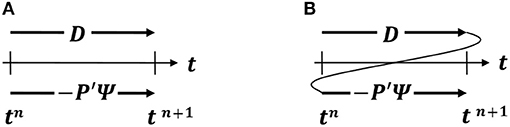
Figure 1. Parallel time splitting (A) and sequential time splitting (B). D represents the dynamics tendency and −P′Ψ represents the physics tendency.

2.2. Sequential Splitting

Sequential splitting, also called time splitting or fractional stepping, is the method where processes are integrated one after the other, but the tendencies from the previous processes are used in the next process (see Figure 1B). For the simple Equation (1), sequential splitting leads to the following finite difference equations:

$\begin{array}{ll}\frac{{\text{Ψ}}^{*}-{\text{Ψ}}^n}{\Delta t}=D({\text{Ψ}}^n),& (6)\end{array}$

$\begin{array}{l}\frac{{\text{Ψ}}^{n+1}-{\text{Ψ}}^{*}}{\Delta t}=-P^{\prime }({\text{Ψ}}^n){\text{Ψ}}^{n+1}\\ or\frac{{\text{Ψ}}^{n+1}-{\text{Ψ}}^n}{\Delta t}=D({\text{Ψ}}^n)-P^{\prime }({\text{Ψ}}^n){\text{Ψ}}^{n+1}.& (7)\end{array}$

The total tendency is:

$\begin{array}{ll}\frac{{\text{Ψ}}^{n+1}-{\text{Ψ}}^n}{\Delta t}=\frac{D({\text{Ψ}}^n)-P^{\prime }({\text{Ψ}}^n){\text{Ψ}}^n}{1+\Delta t{P}^{\prime }({\text{Ψ}}^n)},& (8)\end{array}$

with the steady state solution:

$\begin{array}{ll}{\text{Ψ}}^{n+1}={\text{Ψ}}^n=\frac{D({\text{Ψ}}^n)}{P^{\prime }({\text{Ψ}}^n)}.& (9)\end{array}$

This steady state solution is correct and independent of the time step. The reason is that the implicit process is called last and therefore can achieve a balance with the other process because it “knows” about the tendency of the other process.

Equation (7) can be interpreted in two different ways: (i) Variable Ψ*, updated by the dynamics D(Ψⁿ) is used as starting point of the integration with the physics −P′(Ψⁿ)Ψⁿ, or (ii) D(Ψⁿ) is used as source term in the time integration of the physics. The latter interpretation has the preference, because the first suggests that the physics takes Ψ* as input, which is not entirely correct. If P′ at the right hand side of Equation (7) is evaluated with Ψ*, the steady state solution contains Ψ* rather than Ψⁿ, which leads to a time step dependence. In other words, P′ has to be evaluated at a full time level and not at the “in between” time level between processes. In the case of vertical diffusion P′(Ψⁿ) represents the computation of the diffusion coefficients and they need to be evaluated with full time level profiles.

An interesting and well-known example in meteorology is the process of condensation. Supersaturation with respect to water does not exist in the atmosphere because condensation is so fast that any excess water vapor is instantly converted into water. However, the process of condensation (and evaporation of cloud water) is seldom integrated in time as a short time scale process; instead an iterative procedure is applied to restore saturation at the end of the time step. In fact, this is compatible with sequential splitting. Say dynamics lifts a volume of air above saturation, then an adjustment is made to temperature and moisture in order to reach saturation. The latter is implicit because it is an iterative procedure in which the saturation is evaluated at the new time level, but the tendency of the dynamics has been included in order to have the correct balance.

Time truncation errors can be evaluated by using a short time step integration as a reference. Here we consider the 24 h forecast of wind speed at the lowest model level (10 m) of the ECMWF model with a 60 min time step and compare with a 5 min time step integration. At the lowest model level (in this example) the dominant terms are the pressure gradient (dynamics), the Coriolis term (dynamics) and the turbulent stress divergence. The latter is the fast process that is handled by an implicit computation. Three different schemes are used for the vertical diffusion scheme: (i) parallel splitting, (ii) sequential splitting in which the dynamics tendency is used as source term during the implicit integration of turbulent diffusion, and (iii) sequential splitting as in (ii) but the diffusion coefficients are not computed from time level n, but after the profiles have been incremented with the dynamics. It has been verified that the short time step integrations with all schemes are very similar so they can be used as “truth.” The time truncation errors of the 3 schemes are illustrated in Figure 2 for a T159 integration with a 60 min time step. The errors with parallel splitting (Figure 2A) are systematically positive and large (with a global mean of 0.76 m/s). The reason is that the diffusion scheme decelerates the flow less than it should because through its implicit nature it “sees” a lower velocity at the end of the diffusion time step. Sequential splitting (Figure 2B) is much better and has mixed errors, because the implicit vertical diffusion computation includes the dynamics tendency and therefore achieves a better balance. Sequential splitting with the diffusion coefficient computed after the dynamics increment has been added, has systematic negative errors although the global mean error is not really smaller than with sequential splitting (−0.11 m/s vs. 0.11 m/s). The reason for the reduction in wind speed is that the diffusion coefficients and particularly the transfer coefficients at the lowest model level see a higher wind speed due to dynamics increment (dynamics accelerates the flow and diffusion decelerates it) and due to the higher transfer coefficient, the wind at the lowest model level is reduced more by turbulent diffusion.

FIGURE 2

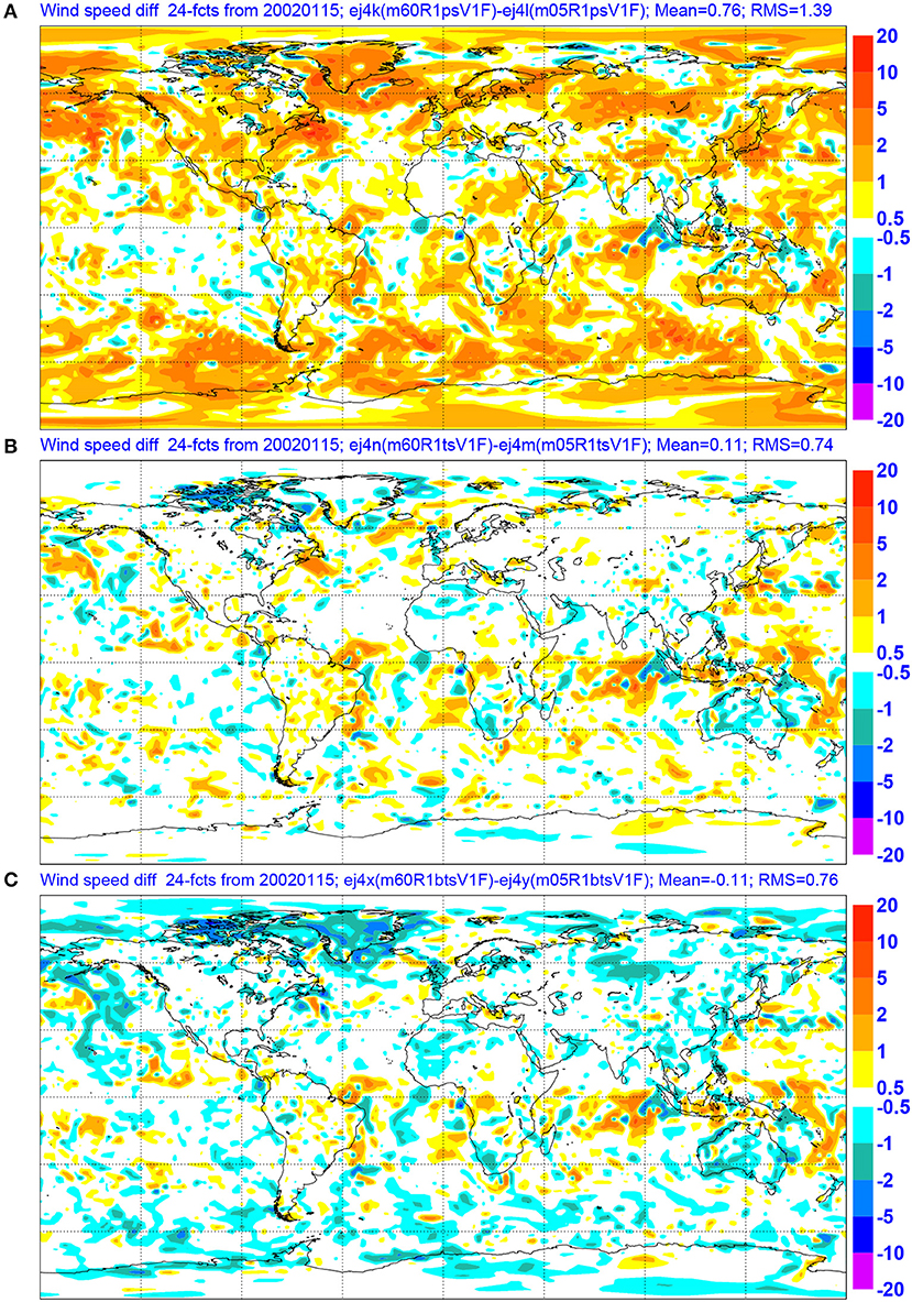
Figure 2. Wind speed (10 m) time truncation errors of a 24 h forecasts with a 60 min time step with different time stepping procedures for the vertical diffusion scheme: (A) parallel splitting (B) sequential splitting and (C) sequential splitting but the diffusion coefficients are computed after the dynamics increments have been added. An integration with a 5 min time step is used as reference (differences between schemes with 5 min time steps are small).

The conclusion to be drawn from these simple examples is that sequential splitting is the preferred option in multiple time scale problems, which is consistent with the more general literature on this topic (e.g., Sportisse, 2000; Williamson, 2002; Dubal et al., 2004; Ropp et al., 2004). Sequential splitting is effective and straightforward in a problem with a single fast (implicit) process. In problems with more than one fast process it would be necessary to combine all fast processes in a single implicit solver to obtain balance within the time step which is in agreement with the findings of Knoll et al. (2003).

2.3. Toward 2nd Order Accuracy in the ECMWF Model

Most models with parametrized physics do time integration of the physics with 1st order splitting methods e.g., explicit forward or implicit backward, and process by process. It is possible to achieve higher order accuracy (e.g., Wicker and Skamarock, 1998; Cullen and Salmond, 2002) but it may be difficult to justify the additional computational costs given the uncertainty in the parametrization. In 1999 a new time stepping scheme has been implemented in the ECMWF model in which an attempt is made to improve the consistency with the dynamical part of the model while enhancing the accuracy of the time stepping, but without increasing the computational burden (Wedi, 1999). The method is called Semi-Lagrangian Averaging of Physical Parametrizations (SLAVEPP). To illustrate the basic principles of SLAVEPP, the following simple equation can be formulated in Lagrangian form

$\begin{array}{ll}\frac{d\text{Ψ}}{dt}=D+P,& (10)\end{array}$

where dΨ/dt denotes the total derivative, D denotes the right hand side of the equations attributed to the dynamical part of the model and P is physics. In the physics we distinguish 5 processes, namely radiation, convection, clouds, vertical diffusion, and subgrid orography. On a discrete mesh, the transported quantity Ψ, which arrives at a gridpoint, and part of D are consistently re-mapped to the departure points of the flow trajectory using a semi-Lagrangian advection algorithm. Here the main focus is now on the evaluation of P which itself depends on Ψ.

The basic idea of SLAVEPP is to approximate P in accord with the dynamical part D, using a second-order trapezoidal rule approximation, where P is evaluated in part at the departure point at time level n and in part at the end of the time step (n + 1) at the arrival point, hence averaging the two tendencies “along” the flow trajectory (see Figure 3). Superscripts d and a are used to indicate departure and arrival points; superscripts n and n + 1 refer to the old and the new time level, and in the semi-Lagrangian sense they should correspond to departure and arrival point, respectively. Because the physics tendency at the arrival point can be interpolated to the departure point for the next time step, the physics needs to be evaluated only once per time step, so there is no extra computational cost and only a moderate increase in storage requirements compared to a simple first-order forward time stepping. The time integration can be represented in the following way:

$\begin{array}{l}\frac{{\text{Ψ}}^{a,n+1}-{\text{Ψ}}^{d,n}}{\Delta t}=D+\frac{1}{2}{P}_{rad+cnv+cld}^{d,n}+\frac{1}{2}{P}_{rad+cnv+cld}^{a,n+1}\\ +P_{vdf+sgo}^{a,n+1},& (11)\end{array}$

where the subscripts rad, cnv, cld, vdf, and sgo refer to the processes radiation, convection, clouds, vertical diffusion and subgrid orography, respectively. Vertical diffusion and subgrid orography are fast processes, so they are evaluated at the new time level (implicit time integration). Wedi (1999) experimented with averaging of vdf + sgo but found large time truncation errors in surface wind over mountainous areas as a result. This suggests that near the surface at locations with high surface stress, the balance between dynamic processes and turbulent friction is more important than the time integration aspect.

FIGURE 3

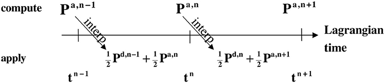
Figure 3. Schematic of Semi-Lagrangian Averaging of Physical Parametrizations (SLAVEPP). P represents the physics tendency.

The accuracy of the resulting scheme depends critically on the ability to evaluate physics tendencies at time level n + 1. Equation (11) suggests that the time integration is implicit in all physical processes which is not feasible with the existing physics codes. Instead, an estimate Ψ* is made of Ψ^{a, n + 1} at the new time level n + 1. The estimate is made by using all the tendencies as far as they have been computed already, and to use the previous time level tendencies for the processes that have not yet been computed. One possible scenario would lead to the following sequence of computations (for simplicity the explicit processes rad/cnv/cld and the implicit processes vdf/sgo have been grouped). First $P_{rad+cnv+cld}^{a,n+1}({\text{Ψ}}^{*})$ is evaluated using

$\begin{array}{ll}{\text{Ψ}}^{*}={\text{Ψ}}^{a,n}+\Delta t\left[D+P_{rad+cnv+cld}^{d,n}+P_{vdf+sgo}^{d,n}\right],& (12)\end{array}$

and then Equation (11) is applied to compute implicitly the tendencies from vdf + sgo.

For a number of reasons, SLAVEPP could not be implemented in the ECMWF model in the way described above: (i) the vertical diffusion (vdf) has to be called before convection (cnv) because surface fluxes are needed by the convection scheme for closure; (ii) to avoid unrealistic boundary layers, vdf + sgo does not use a guess from cld + cnv; and (iii) the basic scheme reduced convective activity in an unacceptable way, so only half of the cnv + cld tendency is applied in Ψ*. The configuration of SLAVEPP that has been implemented, computes tendencies at time level n + 1 sequentially for different processes in the following way

$\begin{array}{ll}{P}_{rad}^{a,n+1}=P_{rad}({\text{Ψ}}^{(1)})with{\text{Ψ}}^{(1)}={\text{Ψ}}^{a,n},& (13)\end{array}$

$\begin{array}{l}{P}_{vdf+sgo}^{a,n+1}=P_{vdf+sgo}({\text{Ψ}}^{(2)})with\\ {\text{Ψ}}^{(2)}={\text{Ψ}}^{a,n}+\Delta t[D+P_{rad}^{a,n+1}+P_{vdf+sgo}({\text{Ψ}}^{(2)})],& (14)\end{array}$

$\begin{array}{l}{P}_{cnv+cld}^{a,n+1}=P_{cnv+cld}({\Psi }^{(3)})with\\ {\Psi }^{(3)}={\Psi }^{a,n}+\Delta t[D+\frac{1}{2}{P}_{rad}^{d,n}+\frac{1}{2}{P}_{rad}^{a,n+1}\\ +P_{vdf+sgo}^{a,n+1}+\frac{1}{2}{P}_{cnv+cld}^{d,n}].& (15)\end{array}$

The total tendency from the physics package is the sum of the result of Equations (13–15). In spite of the compromises in the implementation of SLAVEPP, the scheme is beneficial in the ECMWF model. Wedi (1999) reports a typical reduction of time truncation errors in physics tendencies of up to 25% by comparing long and short time step integrations. This improvement is also seen in the wind speed at the lowest model level (10 m) as shown in Figure 4. The global mean bias is reduced from 0.17 to 0.10 m/s, and the global RMS error is reduced from 0.74 to 0.65 m/s.

FIGURE 4

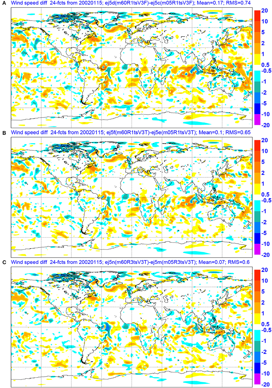
Figure 4. Wind speed (10 m) time truncation errors of 24 h forecasts with a 60 min time step with (A) standard time stepping (B) first implementation of SLAVEPP and (C) revised SLAVEPP with an additional call to the cloud scheme before convection. An integration with a 5 min time step is used as the reference.

2.4. Toward 2nd Order Accuracy in the ECMWF Model: Revised Version

Detailed diagnostics in the EPS (Ensemble Prediction System) which ran at the time of implementation at T255 resolution with a 45 min time step showed a reduction of activity in the convection scheme (leading to more unrealistic gridpoint storms) and a deterioration of scores related to the long time steps. In order to improve, various options in SLAVEPP were explored. As a result, the following configuration of SLAVEPP has been implemented as part of a new model version (CY28R3 implemented 28 September 2004):

$\begin{array}{ll}{P}_{rad}^{a,n+1}=P_{rad}({\text{Ψ}}^{(1)})with{\text{Ψ}}^{(1)}={\text{Ψ}}^{a,n},& (16)\end{array}$

$\begin{array}{l}{P}_{vdf+sgo}^{a,n+1}=P_{vdf+sgo}({\text{Ψ}}^{(2)})with\\ {\text{Ψ}}^{(2)}={\text{Ψ}}^{a,n}+\Delta t[D+P_{rad}^{a,n+1}+P_{vdf+sgo}({\text{Ψ}}^{(2)})],& (17)\end{array}$

$\begin{array}{l}{P}_{cldguess}^{a,n+1}=P_{cld}({\text{Ψ}}^{(3)})with\\ {\text{Ψ}}^{(3)}={\text{Ψ}}^{a,n}+\Delta t[D+P_{rad}^{a,n+1}+P_{vdf+sgo}^{a,n+1}],& (18)\end{array}$

$\begin{array}{l}{P}_{cnv}^{a,n+1}=P_{cnv}({\text{Ψ}}^{(4)})with\\ {\text{Ψ}}^{(4)}={\text{Ψ}}^{a,n}+\Delta t[D+P_{rad}^{a,n+1}+P_{vdf+sgo}^{a,n+1}+\frac{1}{2}{P}_{cldguess}^{a,n+1}],& (19)\end{array}$

$\begin{array}{l}{P}_{cld}^{a,n+1}=P_{cld}({\Psi }^{(5)})with\\ {\Psi }^{(5)}={\Psi }^{a,n}+\Delta t[D+P_{rad}^{a,n+1}+P_{vdf+sgo}^{a,n+1}\\ +P_{cnv}^{a,n+1}+\frac{1}{2}{P}_{cldguess}^{a,n+1}].& (20)\end{array}$

The difference with respect to CY28R1 (compare Equations 19–20 to 15), is in the guess that is made of Ψ at time level n + 1 for the different processes. The revised version does not use the previous time level convection tendency, but has half of the guess of the cloud scheme tendency before entering convection and then it uses the full new convection tendency before computing the tendency from the cloud scheme. The consequence is that the cloud scheme has to be called twice, once to provide a guess for convection and once after convection. The full cloud scheme cannot be called before convection because the cloud scheme needs detrainment from the convection scheme as source term for the cloud variables (Tiedtke, 1993). More recently, it has been realized that in the first call to the cloud scheme, only one element is crucial namely the part where an adjustment to saturation (with respect to water) is applied. Supersaturation or subsaturation in clouds can occur due to tendencies from dynamics or other processes.

Again, the specific configuration of the revised SLAVEPP is inspired by the results, and the benefit can be seen in a variety of diagnostics. Figure 4 shows that the time truncation errors in the surface wind have been reduced (compare Figures 4B,C). This is particularly noticeable in convective areas in the tropics, which suggests that the convective tendencies are handled favorably. Also the tropical winds have improved and the precipitation distribution has become less time step dependent (see Figure 5). The results imply that implicitness is important but inclusion of tendencies (earlier in time or space) from the same parameterized process that is to be simulated (as in Equation 15) appears less beneficial.

FIGURE 5

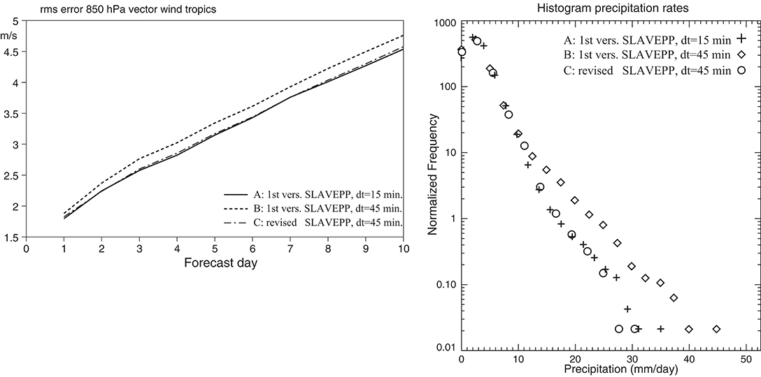
Figure 5. Tropical 850 hPa wind scores (left) and precipitation histogram (right) at T255 resolution with (A) the first version of SLAVEPP and 15-min time step (solid/+), (B) as (A) with a 45-min time step (dotted/◇), and (C) the revised version of SLAVEPP with a 45-min time step (dash-dot/o).

In general it can be concluded that SLAVEPP is beneficial, in spite of the scheme being far from mathematically rigorous. Why the selected configuration in terms of order of processes and selection of estimates of model variables at the arrival point, is better than with Equation (11), is not clear. The distinction between fast and slow processes is probably crucial, and both the convection and cloud schemes combine slow and fast variables. More research is obviously needed, but a way forward may be to separate in the cloud scheme the fast condensation part from the slower processes (e.g., ice deposition). In that way, condensation can be handled at the end of the time step, whereas the slower processes can be averaged over departure and arrival points of the model trajectory. Another positive aspect of 2nd order physics may come from a reduction of noise in the tendencies due to averaging over the trajectory.

3. Process Specific Issues

Subgrid processes all have their specific numerical problems. In this section, numerical issues of the various processes will be discussed in the context of the ECMWF model. Although some of the issues are model specific, many numerical problems are rather general.

3.1. Radiation

Radiation is probably the simplest of all processes from the numerics point of view. In the ECMWF model, temperature, moisture, cloud water/ice and cloud cover are the dynamic fields that are used as input; aerosols, absorbing gases etc. are specified as climatological fields or as constants. The process is fairly slow, so explicit time integration is stable. The fluxes F are computed on half levels based on the profiles at time level n and time integration is performed by computing the flux divergence at every model level j (counted from the top of the model)

$\begin{array}{ll}\frac{dT}{dt}=\frac{g}{C_p}\frac{dF}{dp},& (21)\end{array}$

$\begin{array}{ll}{(T_j^{n+1}-T_j^n)}_{rad}=\Delta t\frac{g}{C_p}\frac{F_{j+1/2}^n-F_{j-1/2}^n}{p_{j+1/2}-p_{j-1/2}},& (22)\end{array}$

with C_p for heat capacity at constant pressure, g for the gravitation constant and p for pressure (which is used as vertical coordinate at half or flux levels).

However, radiation computations are expensive, so in order to save computer time, the computations are done on a coarse grid and interpolated to the full resolution of the model (Morcrette et al., 2008). Furthermore, the full radiation code is not called every time step but every hour in the high-resolution deterministic model configuration, and every 3 h in all other configurations (the medium-range ensemble, monthly and seasonal forecasting, and reanalysis). To obtain tendencies at every time step, some corrections are applied to the broadband flux profiles. In the shortwave, the fluxes computed by full radiation scheme are normalized by incoming solar radiation at top-of-atmosphere. Then at each time step, they are multiplied by incoming solar radiation in order to account for the change in solar zenith angle between calls to the full radiation scheme, leading to a more realistic diurnal cycle. Furthermore, the scheme of Manners et al. (2009) is used to approximately account for the effect on surface fluxes of the change in the path length of direct solar radiation through the atmosphere between calls to the full radiation scheme. In the longwave, the fluxes are modified every time step to account for variation in the skin temperature using the longwave method of Hogan and Bozzo (2015). Before this scheme was introduced, the surface net longwave flux was kept constant between radiation calls, which meant that its response to changing skin temperature was lagged, and in turn the 2-m temperature tended to fall too rapidly during the night in clear-sky conditions.

The use of a coarse radiation grid has in the past led to 2-m temperature errors of up to 10 K at coastlines where there are strong horizontal gradients in skin temperature and surface albedo. These problems were largely solved by the introduction of the Hogan and Bozzo (2015) scheme that performs cheap, approximate updates to the fluxes on the full model grid to account for the high-resolution albedo information in the shortwave, and the high-resolution skin temperature information in the longwave.

The effect of spatial and temporal sampling on forecast skill, after incorporating approximate radiation updates to account for changes in surface properties, was described by Hogan et al. (2017). They reported that reducing the radiation time step from 3 h to 1 h could reduce the root-mean-squared 2-m temperature error by up to 3–4%. This is due to the radiative fluxes responding more rapidly to the change in clouds. By contrast, when the use of a coarse radiation grid was replaced by calling the radiation scheme every model grid point (with 6.25 times more grid points globally, as in the operational ensemble configuration), 2-m temperature errors were improved by only 0.5–1% and even then only up to 2 days into the forecast. This highlights that the model does not predict the location of the clouds more accurately than a few grid spacings, so coarse-graining the clouds by a factor of 2.5 in each horizontal direction in the radiation scheme has a very small impact on forecasts.

With increasing vertical resolution, new radiation related issues arise. A clear example is the radiative flux divergence near a cloud edge. At the top of a thick stratocumulus deck, the main longwave cooling is over a depth of about 10 m. Large scale models have vertical resolution at cloud top of say 200 m so the divergence is spread over one layer only. The typical flux divergence across a stratocumulus top is 80 W/m² leading to a tendency of 35 K/day for a 20 hPa layer. Doubling the resolution will double the tendency in the top cloud layer. The physics of this problem is that radiation cools the cloud top and that turbulent diffusion redistributes this cooling over the entire cloud depth and often the subcloud layer. With long time steps and future high vertical resolution it will probably be necessary to enforce balance between radiation and turbulent diffusion during the time integration. Using sequential splitting may be sufficient, but it might even be necessary to introduce some implicitness in the radiation code for stability.

3.2. Vertical Diffusion

Vertical diffusion describes the effect of vertical transport including the coupling to the surface through turbulence. A popular way of representing turbulent transport is by prescribing eddy diffusion coefficients e.g., as a function of shear and stability (as in the ECMWF model) or with help of a turbulent kinetic energy equation. The equation for model variable Ψ (wind components, dry static energy and specific humidity) reads:

$\begin{array}{ll}\frac{d\text{Ψ}}{dt}=g\frac{dF}{dp},F_{\text{Ψ}}=K_{\text{Ψ}}\rho \frac{d\text{Ψ}}{dz},& (23)\end{array}$

with K_Ψ for the eddy diffusion coefficient which typically depends on Ψ, ρ for density, p for pressure (used for flux levels) and z for height above the surface (used for full levels). Since the time scale of the diffusion process is small near the surface (of the order of 10 s at a height of 10 m), it is necessary to have implicit time stepping for stability. The discretized equations are implicit in the linear part of the equation and explicit in the diffusion coefficient:

$\begin{array}{l}{\text{Ψ}}_j^{*}-{\text{Ψ}}_j^n=\frac{\Delta tg}{\Delta p_j}\left(K_{j+1/2}^n\frac{{\widehat{\text{Ψ}}}_{j+1}-{\widehat{\text{Ψ}}}_j}{z_{j+1}-z_j}-K_{j-1/2}^n\frac{{\widehat{\text{Ψ}}}_j-{\widehat{\text{Ψ}}}_{j-1}}{z_j-z_{j-1}}\right)\\ +{(\Delta \text{Ψ})}_{dyn}+{(\Delta \text{Ψ})}_{rad},& (24)\end{array}$

$\begin{array}{ll}with\widehat{\text{Ψ}}=\alpha {\text{Ψ}}^{*}+(1-\alpha ){\text{Ψ}}^n,with\alpha =1.5.& (25)\end{array}$

The dynamics and radiation tendencies are used as source term in the time integration of vertical diffusion. As shown in section Time Stepping, this is essential to achieve balance between processes. The balance between pressure gradient, Coriolis term and vertical diffusion ensures bias free surface winds for long time steps and the balance between radiative cooling and turbulent transport in cloud layers is essential to have time step independent solutions near cloud tops.

Another major issue in relation to vertical diffusion is numerical stability. Although fully implicit time integration (i.e., α = 1 in Equation 25), ensures absolute stability in a linear system, non-linear instabilities can still occur in case the diffusion coefficients (which are computed explicitly) depend strongly on the model variables. This is indeed the case in the atmosphere; the diffusion coefficients are a strong function of shear and stability. Particularly the transition from stable to unstable is very pronounced, with diffusion being weak in stable situations and strong in unstable situations. The classic paper by Kalnay and Kanamitsu (1988) discusses the problem extensively using a simple ordinary non-linear differential equation as an example. They analyze stability of a number of schemes e.g., predictor corrector, over-implicit and fully implicit based on linearized diffusion coefficients. The latter is absolutely stable but difficult to implement. Predictor-corrector appears attractive, but does not always give the correct result (see also McDonald, 1998). An over-implicit scheme (e.g., with α = 1.5) seems to be a good compromise between simplicity and effectiveness. Girard and Delage (1990) use the implicitness factor in a dynamic way by selecting a value that depends on a local stability criterion. More complicated schemes can be beneficial, but usually add to the costs (Hammarstrand, 1997; Wood et al., 2007).

The problem of non-linear instability does not only manifest itself as fatal blow-ups, but can also be seen sometimes as finite amplitude noise. Different authors report noise in atmospheric models and claim advantages of one scheme over the other (e.g., Beljaars, 1991; Janssen and Doyle, 1997). However, noise due to the non-linear vertical diffusion equation is quite common but erratic. Improvements may be seen in one situation whereas more noise may occur in another case.

In order to get a more global perspective in the ECMWF system, the RMS of dU/dt (zonal wind) is computed as a global field over the first 24 h of a forecast. In Figures 6A,B parallel and sequential splitting are compared and it is clear that parallel splitting is very noisy, particularly in the storm tracks of the Northern and Southern Hemisphere. Figure 6C clearly shows the finite amplitude 2Δt noise, which is typical for the non-linear instability. The point where the diffusion coefficient is computed (e.g., after the dynamics tendency has been added) has little impact in contrast with earlier suggestions (Hammarstrand, 1997). Whether these results are universal is difficult to say, because the interaction of the non-linear instability with the splitting scheme is not well understood and may depend on various details of numerics and dynamics.

FIGURE 6

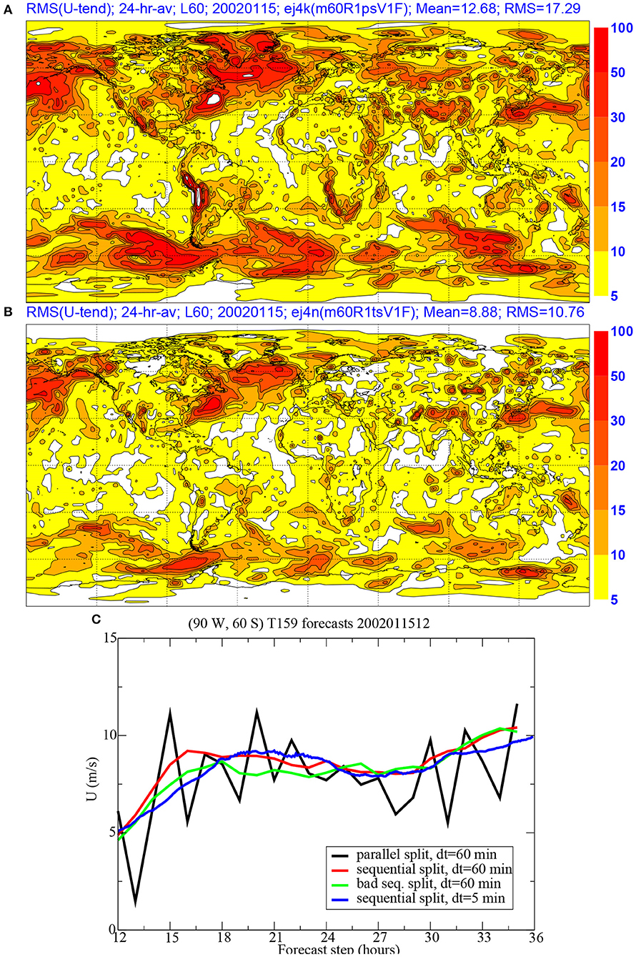
Figure 6. RMS of the zonal wind speed tendency [RMS(dU/dt)] at the 10 m level with (A) parallel splitting for vertical diffusion, and (B) sequential splitting. The units are ms⁻¹day⁻¹. The RMS is obtained by averaging over the first 24 h of a T159 forecast with a 60 min time step. (C) represents time series of zonal wind (every time step) at 60^oS/90^oW with parallel splitting (black) sequential splitting (red), sequential splitting with diffusion coefficient after dynamics has been added (green), and sequential splitting with a 5 min. time step (blue).

Another numerical issue related to vertical diffusion is vertical resolution. One would expect strong sensitivity to resolution in the stable boundary layer because the stable boundary layer has a lot of structure in a shallow layer (typically 200 m deep). Surprisingly, resolution has little impact on the simulation of the stable boundary layer. The numerical handling of the surface layer is probably an important aspect, because the finite differencing in the surface layer uses similarity profiles (instead of the linear finite differencing above the surface layer) which is exact in the constant flux layer. The lack of sensitivity of the stable boundary to resolution was found by Beljaars (1991) and confirmed by Cuxart et al. (2004) in an inter-comparison study.

On the other hand, resolution does have impact on inversion structure. Figure 7 shows a simulation with the ECMWF single column model at operational resolution (typically 200 m at inversion level) and at 10 m resolution. This is a stratocumulus case with a very steep inversion; steps of 10 K in temperature and 10 g/kg in specific humidity are typical. As expected, resolution affects the sharpness of the inversion and the details of the time evolution of its height. As explained in section Radiation, radiative cooling at cloud top and vertical diffusion balance each other. Such a balance is achieved by having the radiative tendency at the right hand side of Equation (24) as a source term.

FIGURE 7

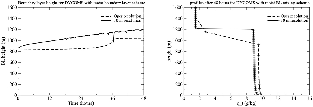
Figure 7. Time evolution of inversion height (Left) and vertical profile of specific humidity (Right) from single column simulations with the ECMWF model of a stratocumulus case with operational resolution (typically 200 m at inversion height, dashed) and 10 m resolution (solid).

Resolution is not the only cause for numerical errors at sharp inversions. With the inversion resolved as a transition between two levels, numerical diffusion can overwhelm the physics in the parametrization as reported by Lenderink and Holtslag (2000). These inversions tend to be rather stationary and are the result of a balance between downward large scale motion (typical subsidence rates are 0.5 cm/s) and entrainment by turbulence moving the inversion up with the same speed as the large scale subsidence. Since the inversion is strong, entrainment corresponds to a small diffusion coefficient, so numerical diffusion can easily dominate the entrainment. Lenderink and Holtslag (2000) showed that standard numerical methods have a tendency to “lock in” on the grid where entrainment always equals vertical velocity independent of the parametrization assumption. In order to obtain a realistic inversion evolution, Lock (2001) and Grenier and Bretherton (2001) developed special methods to represent the inversion dynamics. Lock (2001) makes an estimate of the numerical errors in vertical advection and adjusts the parametrized entrainment accordingly. Alternatively, Suarez et al. (1983) use a mixed-layer approach with the boundary layer (BL) top being a coordinate surface. This has the advantage of a simple treatment of the BL top entrainment as well as its interaction with convection. It has been recently extended to relax the mixed-layer assumption while introducing multiple layers within the BL.

3.3. Subgrid Orography

The subgrid orography scheme in the ECMWF model developed by Lott and Miller (1997), consists of two parts: (i) the low level blocking part and (ii) the gravity wave part. The low level blocking part provides strong surface drag with momentum extracted from the low level flow. The gravity wave part also leads to surface drag but the momentum exchange is with higher levels through gravity wave breaking. The surface stress associated with this scheme can be very large in mountainous areas (up to 10 N/m²). These very high numbers often occur at isolated points which may lead to unrealistic effects in adjacent points through numerical smoothing of the fields.

Because of the strong tendencies at the lowest model levels, the scheme has to be implicit to ensure numerical stability. Numerically, the same procedure is adopted as for the vertical diffusion solver: the drag coefficients are prescribed explicitly and the linear part is treated implicitly. Initially, vertical diffusion and subgrid orography were integrated separately, but it resulted in a time step dependence because the two processes both have short time scale near the surface and by having them separately, they cannot reach a balance. To avoid this, vertical diffusion and subgrid orography are integrated together now in the same tridiagonal solver. It ensures balance between the fast processes and the dynamics (Orr, 2007).

3.4. Convection

The convection scheme in the ECMWF model uses a bulk mass flux approach (derived from Tiedtke, 1989) for up- and down-drafts. Here we consider only the updraught in the convection tendency for variable Ψ:

$\begin{array}{ll}\frac{d\text{Ψ}}{dt}=g\frac{d}{dp}\left[M_u({\text{Ψ}}_u-\text{Ψ})\right]+S,& (26)\end{array}$

where M_u is the updraught mass flux, Ψ_u the updraught property, and S a possible source term for e.g., latent heat release due to condensation. Although ECMWF solves for wind, tracers, dry static energy and specific humidity, from the numerical point of view, variable Ψ can be thought of as a moist conserved variable i.e., moist static energy and total water. The conversion expressions are ignored here for simplicity. The properties of the updraught Ψ_u are computed by an additional ordinary differential equation. A parcel with initial perturbations proportional to surface fluxes is followed on its way upwards by considering buoyancy, entrainment, and condensation. Entrainment and detrainment determine the mass flux profile and cloud base mass flux is scaled with the amount of instability for deep convection (CAPE) and with subcloud moist static energy convergence for shallow convection (Bechtold et al., 2008). These parametrization assumptions require a link with the vertical diffusion scheme for the surface fluxes. The latter is the motivation to call the vertical diffusion scheme before the convection scheme. The mass flux closure for deep convection is designed in such a way that it decreases CAPE over a prescribed time scale. The time scale depends on model resolution and is typically 1 h at low resolution (say 100 km) and 15 min at high resolution (say 10 km). This time scale is of the order of the time step which makes it difficult from the numerical point of view to classify the process as fast or slow. Although Equation (26) is valid below cloud base, it is not used there, but instead the fluxes are prescribed by linear interpolation between cloud base and the surface.

With prescribed Ψ_u and M_u profiles, Equation (26) is solved with an upwind differencing scheme:

$\begin{array}{l}{\left({\Psi }_j^{n+1}-{\Psi }_j^n\right)}_{cnv}=\frac{\Delta tg}{\Delta p_j}[{(M_u{\Psi }_u)}_{j+1/2}-{(M_u{\Psi }_u)}_{j-1/2}\\ -{(M_u)}_{j+1/2}{\Psi }_j+{(M_u)}_{j-1/2}{\Psi }_{j-1}]+\Delta t{S}_j.& (27)\end{array}$

The numerical solution of this advection equation is only stable if the mass flux (equivalent to an advection velocity) is sufficiently small in order not to violate the CFL criterion (M_u < Δp/gΔt). Such a limit is explicity imposed in the mass flux closure. However, the limit alters the parametrization at high vertical resolution and long time steps, which is undesirable. In Figure 8 zonal mean mass flux profiles are shown for time steps of 15 and 45 min. It indicates that the mass flux limiter is very active, resulting in much smaller mass fluxes with 45-min time steps than with 15 min. Mass fluxes in the lower troposphere tend to be high due to shallow convection and are limited by the CFL criterion.

FIGURE 8

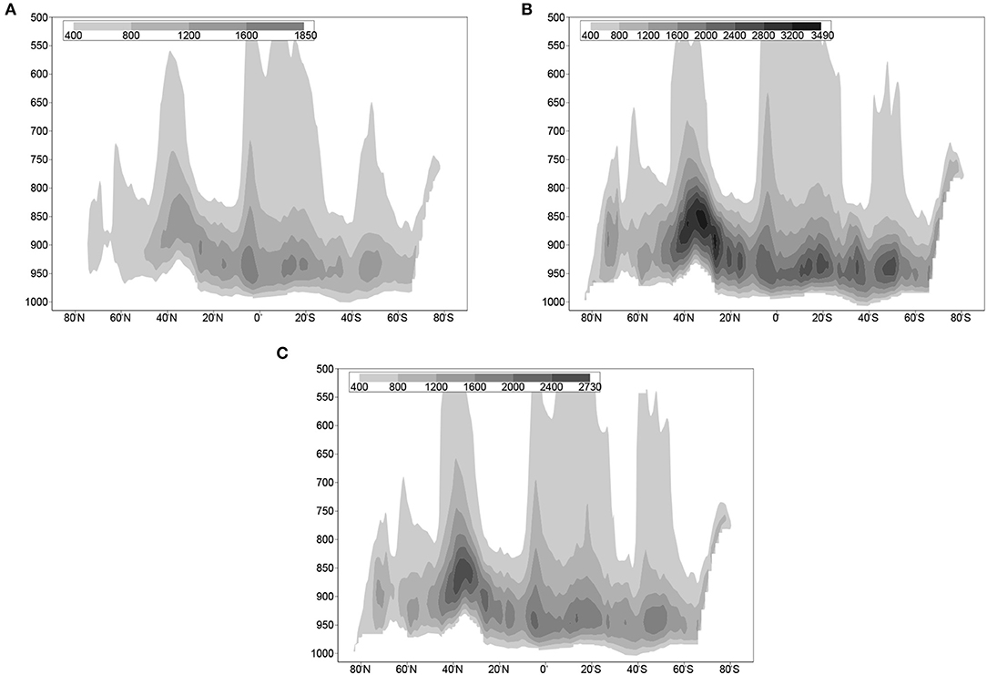
Figure 8. Zonally averaged mass fluxes as a function of pressure from a T255 forecast with a 45 min time step (A), a 15 min time step (B), and with a modification in which the mass flux limit has been relaxed (possible through the implicit formulaton) by a factor 3 for shallow convection and a 45 min time step (C). The units are kgm⁻²day⁻¹.

With increasing vertical resolution and more emphasis on the parametrization of boundary layer clouds it is not possible any more to have explicit time integration for convection. Therefore, in the ECMWF model, the explicit formulation of Equation (27) has been replaced by a formulation where Ψ at the right hand side is treated implicitly (Bechtold et al., 2008). Updraught properties and mass fluxes are still precomputed and prescribed explicitly. Although rather simple in principle, complications do arise from the fact that Ψ_u is itself a non-linear function of Ψ. Therefore, the implicit formulation is not absolutely stable. In practice, the CFL limit could be relaxed by about a factor 3 in the ECMWF model. Figure 8C shows that this reduces the activity of the CFL limiter and therefore the time step dependence. An implicit mass flux term was also successfully implemented in a new boundary layer scheme for dry boundary layers and stratocumulus mixing processes (Tompkins et al., 2004).

3.5. Clouds

The cloud scheme in the 2004 version of the ECMWF model had two prognostic variables, namely the combined cloud water/ice variable ℓ and cloud cover a (Tiedtke, 1993). The scheme uses source and sink terms from dynamics, radiation, convection, vertical diffusion and adds processes like precipitation and cloud erosion. Cloud processes are notoriously difficult to integrate in time because of the short time scales of some of the processes particularly the microphysics. To obtain a stable scheme, the prognostic equations are written in the following form

$\begin{array}{ll}\frac{d{l}}{dt}=C-D{l},& (28)\end{array}$

$\begin{array}{ll}\frac{da}{dt}=A-Ba,& (29)\end{array}$

where the different processes contribute to the coefficients A, B, C, and D. These equations are integrated analytically over a time step which leads to an exponential solution. Tompkins et al. (2004) discuss in more detail the numerics of the cloud scheme and its sensitivity to some upgrades. The ice fallout formulation is particularly sensitive and therefore we will discuss it here. A typical situation is an ice source term from convective detrainment and a sink term due to ice settling. The balance between the two processes controls the ice water content which is relevant for the radiation computation. The rate equation for ℓ in this situation reads

$\begin{array}{ll}\frac{d{l}}{dt}=\frac{1}{\rho }{D}_{up}({{l}}_u-{l})-\rho g{w}_{ice}\frac{d{l}}{dp},w_{ice}=c_1{{l}}^{c_2}.& (30)\end{array}$

The first term is the source term from the detrainment of the convection updraught with ℓ_u for updraught ice water, and D_up the mass detrainment rate. The second term is the ice settling term, with the ice vertical velocity w_ice parametrized as a non-linear function of ℓ. The coefficients C and D for level j are defined as follows

$\begin{array}{ll}C=\frac{1}{\rho }{D}_{up,j}({{l}}_{u,j}-{{l}}_j)-{\rho }_{j-1}g{w}_{ice,j-1}\frac{{{l}}_{j-1}}{\Delta p_{j-1}},& (31)\end{array}$

$\begin{array}{ll}D=-{\rho }_{j}g{w}_{ice,j}\frac{1}{\Delta p_j}.& (32)\end{array}$

This numerical formulation is by no means obvious and is inspired by practical considerations and the requirement of conservation. The convection detrainment term has been evaluated already in the convection scheme so it is taken as an explicit source. The ice settling velocity is a non-linear function of ℓ and is evaluated from ℓ at the old time level. The ice settling term is evaluated from top to bottom, i.e., what is falling out of a layer is computed implicitly and this amount is used as an explicit source term in the layer below. This has the advantage that conservation is always guaranteed. To obtain a proper equilibrium between the convective source term, the ice falling into the layer from above and the ice settling toward lower layers, it is essential to have all the source terms in the implicit calculation. Whether the layer by layer formulation is optimal is subject of further research.

In 2010, a major upgrade of the parametrization of stratiform clouds and precipitation was made in the operational system (Forbes et al., 2011). Three additional prognostic variables were introduced to enable a more physically based representation of mixed-phase clouds (liquid/ice) and precipitation (liquid/solid). A fully implicit method is employed to solve the network of microphysics pathways stably for long timesteps. This involves the inversion of a 5 × 5 matrix for each model level corresponding to the variables for water vapor, cloud liquid water, cloud ice, rain and snow.

3.6. Land Surface Scheme

Land surface schemes are used to provide a boundary condition for temperature and moisture over land. In contrast to the ocean where the sea surface temperature has a small diurnal cycle, over land the boundary condition is a combination between fluxes and temperature. During daytime the boundary condition has the character of a flux condition controlled by radiation and Bowen ratio, the latter depending on soil moisture.

Typically land surface schemes, calculate the energy and water balance in the soil by solving for diffusion type equations for temperature and soil moisture. These equations are non-linear because the diffusion coefficients and hydraulic properties depend on soil moisture. An example is the TESSEL scheme (Tiled ECMWF Scheme for Surface Exchanges over Land; Van den Hurk et al., 2000), which has 4 soil layers, tiles for a simple description of surface heterogeneity, a snow module (Dutra et al., 2010), an interception reservoir for fast evaporation of water on top of the vegetation and bare soil and a skin layer without heat capacity for instantaneous temperature response to the forcing by radiation and other components of the surface energy balance.

For the numerical aspects it is important to realize that soil and vegetation properties are highly uncertain and variable even within a grid box. It is therefore difficult to justify very accurate and potentially expensive numerical methods. The emphasis is on stability, conservation of water and energy, a representation of time scales from hours to a year, and on a crude representation of the soil profiles. Therefore, the vertical structure is simulated with a few layers only. Figure 9 illustrates the phase and amplitude errors due to the finite vertical resolution in the TESSEL scheme with 4 layers (7, 21, 72, and 189 cm) as a function of frequency for sinusoidal forcing (Viterbo, 1996). The layer depths have been optimized to keep errors under control over a wide range of time scales within the constraint of a very limited number of layers. Further features of the TESSEL numerics are the implicit solver for the diffusion equations for soil moisture and temperature and an implicit coupling of the skin temperature with the vertical diffusion tridiagonal solver.

FIGURE 9

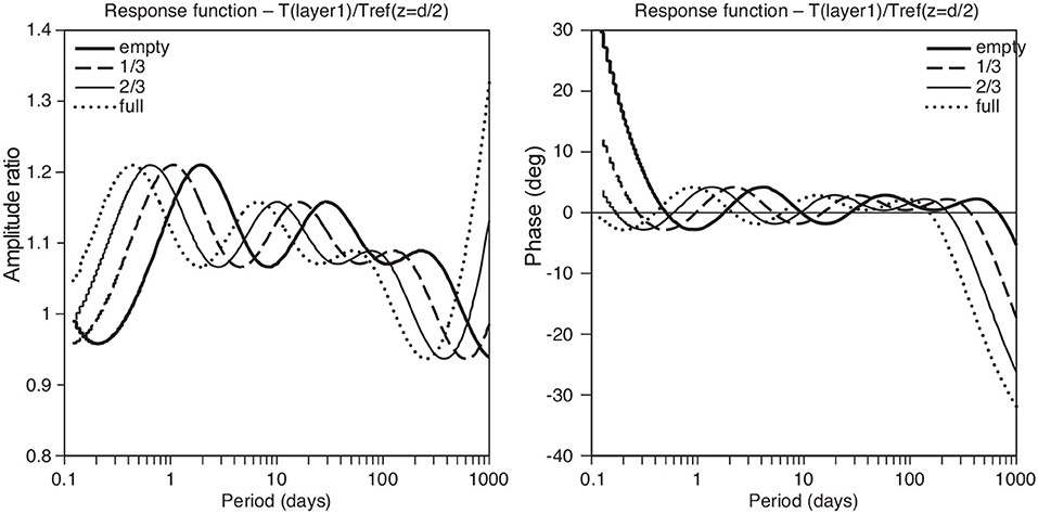
Figure 9. Amplitude ratio and phase error (degrees) of the layer-1 solution of the discretized soil temperature equations with layer depths of 7, 21, 72, and 189 cm for sinusoidal forcing with different frequencies. The errors are with respect to the analytical reference solution of the non-discretized diffusion problem (ratio 1 and a phase error of 0° indicate the exact solution). Four different constant diffusion coefficients are used corresponding to the soil moisture range from permanent wilting point (empty soil reservoir) to field capacity (full reservoir).

3.7. Atmosphere Land Coupling

Coupling between the vertical diffusion and land surface schemes deserves particular attention, because processes in the boundary layer as well as near the surface in the land surface scheme have short times scales and therefore require implicit numerics. In the TESSEL scheme, the surface skin temperature has fully implicit coupling with the vertical diffusion scheme. This is achieved by solving for the surface energy balance between the downward elimination sweep of the vertical diffusion tri-diagonal matrix and the upward back substitution. The tile scheme raises additional difficulties which are solved in TESSEL by computing a skin temperature for each tile from its surface energy balance as if the tile occupies the entire grid box. Then, the skin temperatures are kept fixed and tile averaged fluxes are computed. This procedure is only implicit for the dominant tiles and not for the tiles that occupy small fractions.

More recently, a revised coupler has been introduced as proposed by Best et al. (2004). It has the advantage of being fully implicit on all tiles and it allows for a “universal” way of coupling land surface schemes with atmospheric models. The latter aspect is important, because it provides a framework in which land surface schemes can be exchanged between models without too much difficulty. Because of its practical importance, we give a brief description here (see (Best et al., 2004) for more details).

We start with the description of the surface energy balance for each tile. The turbulent fluxes are expressed in terms of differences between the lowest model level dry static energy $\widehat{S_l}$ (S = C_pT + gz) and specific humidity $\widehat{q_l}$ and their corresponding skin values

$\begin{array}{ll}H=\rho C_H^n\left|{\overrightarrow{U}}_l^n\right|\left[{\widehat{S}}_l-{\widehat{S}}_{sk}\right],& (33)\end{array}$

$\begin{array}{ll}E=\rho C_Q^n\left|{\overrightarrow{U}}_l^n\right|{\beta }_s\left[{\widehat{q}}_l-{\alpha }_s{\widehat{q}}_{sat}({\widehat{T}}_{sk})\right],& (34)\end{array}$

where $C_H^n$ and $C_Q^n$ are the transfer coefficients for heat and moisture, $\left|{\overrightarrow{U}}_l^n\right|$ is the absolute wind speed at the lowest model level and α_s, β_s are the coefficients that control the moisture availability at the surface through parametric relations with e.g., soil moisture. Note that the implicit variables of the vertical diffusion scheme have been used. They can be fully implicit or extrapolated in time (over-implicit) dependent on coefficient α (see Equation 25). If the variables are extrapolated in time, the consequence is that the surface skin temperature will also be extrapolated in time. The surface energy balance reads:

$\begin{array}{ll}H+LE+R_{SW}+R_{LW}=\Lambda ({\widehat{T}}_{sk}-T_s^n).& (35)\end{array}$

Parameter L is the latent heat of evaporation, R_SW and R_LW are the net shortwave and longwave radiative fluxes, and the right hand side of Equation (35) represents the ground heat flux through the skin layer conductivity Λ and the difference of the skin temperature with the first soil layer $T_s^n$ (taken from the old time level). Although this formulation looks rather specific for TESSEL, it can be generalized quite easily by e.g., including an inertia term dT_sk/dt.

The next step is to linearize $q_{sat}({\widehat{T}}_{sk})$ with respect to the previous time level skin temperature $T_{sk}^n$ and to eliminate ${\widehat{T}}_{sk}$ from Equations (33, 34) using (35). This results in two equations expressing the relation between turbulent fluxes and lowest model level variables in the following form:

$\begin{array}{ll}H=D_{H1}{\widehat{S}}_l+D_{H2}{\widehat{q}}_l+D_{H3},& (36)\end{array}$

$\begin{array}{ll}E=D_{E1}{\widehat{S}}_l+D_{E2}{\widehat{q}}_l+D_{E3},& (37)\end{array}$

with coefficients D that can be computed explicitly from the old time level variables. The averaging over tiles reduces to an averaging over coefficients because the lowest model level variables are assumed to be independent of the tiles. The grid box averaged fluxes read

$\begin{array}{ll}\overline{H}={\widehat{S}}_l{\displaystyle \sum _i}{\nu }^i{D}_{H1}^i+{\widehat{q}}_l{\displaystyle \sum _i}{\nu }^i{D}_{H2}^i+{\displaystyle \sum _i}{\nu }^i{D}_{H3},& (38)\end{array}$

$\begin{array}{ll}\overline{E}={\widehat{S}}_l{\displaystyle \sum _i}{\nu }^i{D}_{E1}^i+{\widehat{q}}_l{\displaystyle \sum _i}{\nu }^i{D}_{E2}^i+{\displaystyle \sum _i}{\nu }^i{D}_{E3},& (39)\end{array}$

with superscript i indicating the tile index and νⁱ representing the tile fraction assuming that ${\Sigma }_i{\nu }^i=1$. Equations (38, 39) can be combined with the result of the downward elimination sweep of the vertical diffusion tridiagonal matrix which is also a relation between lowest model level variables and surface fluxes:

$\begin{array}{ll}{\widehat{S}}_l=A_s\overline{H}+B_s,& (40)\end{array}$

$\begin{array}{ll}{\widehat{q}}_l=A_q\overline{E}+B_q.& (41)\end{array}$

Equations (38, 39 and 40, 41) can now be solved for $\bar{H}$, Ē, Ŝ_l, and ${\widehat{q}}_l$, after which the solution of the tri-diagonal matrix can be completed by an upward back substitution. In this procedure the vertical diffusion solver straddles the surface scheme.

In spite of the complicated coupling, the procedure outlined above, leads to a clean coupling strategy between atmospheric and land surface models. As suggested by Best et al. (2004), the atmospheric model provides the A and B coefficients from Equations (40, 41) to the land surface model and the land surface model returns fluxes (see Figure 10). In this coupling, the atmosphere and land are separated at the lowest model level and the atmospheric surface layer is considered to be part of the land surface scheme. Also the complications of surface heterogeneity as reflected by the tile structure are only seen by the land surface model. The implicit tile coupling as described above has been implemented in the ECMWF model with model cycle 28R3 (introduced 28 Sep 2004). The scheme reduces noise for tiles with small fractions as illustrated in Figure 11.

FIGURE 10

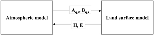
Figure 10. Exchange of parameters between atmospheric models and land surface schemes for universal coupling (Best et al., 2004).

FIGURE 11

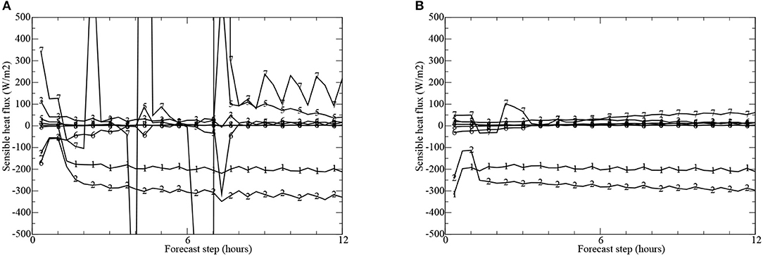
Figure 11. Time series of sensible heat flux (Wm⁻²) for the 8 TESSEL tiles from a 12 h forecast in NE Siberia with implicit coupling for the dominant tile only (A) and the fully implicit coupling on all tiles according to Best et al. (2004) (B). The fractional cover of the tiles for this point is: 1. water: 0.0; 2. ice: 0.0; 3. wet interception: 0.53; 4. low vegetation: 0.04; 5. exposed snow: 0.00; 6. high vegetation: 0.37; 7. snow under high vegetation: 0.00; 8. bare oil: 0.06. Note that fluxes are also computed for tiles that are not relevant or active at a particular time (i.e., have fractional cover 0).

The coupling between the skin layer and the underlying soil or snow layer is treated with explicit flux coupling, i.e., the heat flux between the skin and the soil/snow is computed from the soil/snow temperatures at the previous time level whereas the skin temperature is from the new time level. This explicit coupling can lead to an instability of the first soil/snow layer if the latter is very thin. Most of the time it is not a problem, except in case of very thin snow (after first snow fall or during snow melt). This problem can be solved by including the first soil or snow layer as part of the implicit solution process. However, it has the disadvantage that codes become highly coupled and less modular. As a compromise, a scheme has been developed by Beljaars et al. (2017) where the new soil/snow temperature is anticipated by making use of a similarity solution of the diffusion equation. It is in fact a parametrization of the implicit solution without compromising the modularity of the code.

4. Concluding Remarks

The numerics of physical parametrization has been discussed mainly in the context of the ECMWF Integrated Forecasting System. Parametrization schemes have a modular design and therefore splitting techniques are essential for the time stepping. Two major splitting techniques have been discussed: parallel splitting and sequential splitting. It is argued that sequential splitting is best with the explicit processes first and the implicit processes last. It is essential for the implicit process to have the tendencies of the other processes as input, otherwise it is not possible to obtain a proper balance for long time steps. Sequential splitting in multiple time scale problems can only work well with a single implicit process which is used last. With more than one fast process, it is desirable to combine them in a single solver.

Numerical integration of parametrized processes is typically first order accurate only. In the ECMWF model an attempt has been made to move toward 2nd order accuracy without increasing the costs. The idea is to average the parametrized tendencies “along” the semi-Lagrangian trajectory. The method is successful as it decreases time truncation errors. However, some questions remain. Details of the formulation needed “optimization” to get good results, which is not satisfactory. An essential distinction has to be made between slow and fast processes in the design of the scheme. At this stage it is not clear in what category convection and clouds should be, because they contain time scales of the order of the time step as well as very fast processes. Further research is necessary to find optimal handling of these processes in the context of 2nd order physics.

A review of the numerical aspects of parametrized processes in the ECMWF model is given. Different processes have different numerical problems. However, in order to design the numerics it is important to have a good insight into the physics of the problem and to have an understanding of how the different processes interact. Future increase in horizontal and vertical resolution will be even more demanding on the numerics and may require substantial effort to ensure stability and accuracy for long time steps.

Author Contributions

ABe wrote the paper. The other authors with expertise on individual processes, provided input on these processes (GB and PV on land surface processes, PB on convection, ABo, RH, and J-JM on radiation, RF and AT on clouds, MK on boundary layer). NW provided input on the SLAVEPP scheme.

Conflict of Interest Statement

The authors declare that the research was conducted in the absence of any commercial or financial relationships that could be construed as a potential conflict of interest.

Acknowledgments

We are grateful for the constructive and detailed comments by three reviewers. Their input led to substantial improvement of the manuscript. The original version of this paper was presented by the first author at the 2004 ECMWF Annual Seminar on Recent developments in numerical methods for atmosphere and ocean modeling. ECMWF has given permission to submit the paper to Frontiers in Earth Science, section Atmospheric Science.

References

Bechtold, P., Köhler, M., Jung, T., Doblas-Reyes, F., Leutbecher, M., Rodwell, M. J., et al. (2008). Advances in simulating atmospheric variability with the ECMWF model: from synoptic to decadal time-scales. Q. J. R. Meteor. Soc. 134, 1337–1351. doi: 10.1002/qj.289

CrossRef Full Text | Google Scholar

Beljaars, A. (1991). “Numerical schemes for parametrizations, ECMWF Seminar proceedings 9-13 September 1991,” in Numerical Methods in Atmospheric Models, Vol II, 1–42. Available online at: https://www.ecmwf.int/sites/default/files/elibrary/1991/8028-numerical-schemes-parametrizations.pdf

Google Scholar

Beljaars, A., Dutra, E., Balsamo, G., and Lemarié, F. (2017). On the numerical stability of surface-atmosphere coupling in weather and climate models. Geosci. Model Dev. 10:977. doi: 10.5194/gmd-10-977-2017

CrossRef Full Text | Google Scholar

Bénard, P., Vivoda, J., Masek, J., Smolková, P., Yessad, K., Smith, C., et al. (2010). Dynamical kernel of the Aladin-NH spectral limited-area model: Revised formulation and sensitivity experiments. Q. J. R. Meteor. Soc. 136, 155–169. doi: 10.1002/qj.522

CrossRef Full Text | Google Scholar

Best, M. J., Beljaars, A., Polcher, J., and Viterbo, P. (2004). A proposed structure for coupling tiled surfaces with the planetary boundary layer. J. Hydr. Meteor. 5, 1271–1278. doi: 10.1175/JHM-382.1

CrossRef Full Text | Google Scholar

Browning, G. L., and Kreiss, H.-O. (1994). Splitting methods for problems with different time scales. Mon. Wea. Rev. 122, 2614–2622. doi: 10.1175/1520-0493(1994)122<2614:SMFPWD>2.0.CO;2

CrossRef Full Text | Google Scholar

Caya, A., Laprise, R., and Zwack, P. (1998). Consequences of using the splitting method for implementing physical forcings in a semi-implicit semi-Lagrangian model. Mon. Wea. Rev. 126, 1707–1713. doi: 10.1175/1520-0493(1998)126<1707:COUTSM>2.0.CO;2

CrossRef Full Text | Google Scholar

Cullen, M. J. P., and Salmond, D. J. (2002). On the Use of a Predictor-corrector Scheme to Couple the Dynamics With the Physical Parametrizations in the ECMWF Model. ECMWF Technical Memo no. 357. Available online at: https://www.ecmwf.int/sites/default/files/elibrary/2002/8842-use-predictor-corrector-scheme-couple-dynamics-physical-parametrizations-ecmwf-model.pdf

Cuxart, J., Holtslag, A. A. M., Beare, R. J., Bazile, E., Beljaars, A., Cheng, A., et al. (2004). Single-column model intercomparison for a stably stratified atmospheric boundary layer. Bound.-Layer Meteor. 118, 273–303. doi: 10.1007/s10546-005-3780-1

CrossRef Full Text | Google Scholar

Dubal, M., Wood, N., and Staniforth, A. (2004). Analysis of parallel versus sequential splittings for time-stepping physical parametrizations. Mon. Wea. Rev. 132, 121–132. doi: 10.1175/1520-0493(2004)131<0121:AOPVSS>2.0.CO;2

CrossRef Full Text | Google Scholar

Dubal, M., Wood, N., and Staniforth, A. (2006). Some numerical properties of approaches to physics-dynamics coupling for NWP. Q. J. R. Meteor. Soc. 132, 27–42. doi: 10.1256/qj.05.49

CrossRef Full Text | Google Scholar

Dutra, E., Balsamo, G., Viterbo, P., Miranda, P. M., Beljaars, A., Schär, C., et al. (2010). An improved snow scheme for the ECMWF land surface model: description and offline validation. J. Hydrometeor. 11, 899–916. doi: 10.1175/2010JHM1249.1

CrossRef Full Text | Google Scholar

ECMWF (2008). “Parametrization of subgrid physical processes”, in ECMWF Seminar Proceedings. Available online at: https://www.ecmwf.int/en/learning/workshops-and-seminars/past-workshops/2008-annual-seminar

ECMWF (2015). “Physical processes in present and future large scale models,” in ECMWF Seminar Proceedings. Available online at: https://www.ecmwf.int/en/learning/workshops-and-seminars/past-workshops/annual-seminar-2015

Forbes, R. M., Tompkins, A. M., and Untch, A. (2011). A new prognostic bulk microphysics scheme for the IFS. ECMWF Technical Memo No. 649. Available online at: https://www.ecmwf.int/sites/default/files/elibrary/2011/9441-new-prognostic-bulk-microphysics-scheme-ifs.pdf

Girard, C., and Delage, Y. (1990). Stable schemes for the vertical diffusion in atmospheric circulation models. Mon. Wea. Rev. 118, 737–746. doi: 10.1175/1520-0493(1990)118<0737:SSFNVD>2.0.CO;2

CrossRef Full Text | Google Scholar

Grenier, H., and Bretherton, C. S. (2001). A moist PBL parametrization for large-scale models and its application to subtropical cloud-topped marine boundary layers. Mon. Wea. Rev. 129, 357–377. doi: 10.1175/1520-0493(2001)129<0357:AMPPFL>2.0.CO;2

CrossRef Full Text | Google Scholar

Gross, M., Malardel, S., Jablonowski, C., and Wood, N. (2016b). Bridging the (knowledge) gap between physics and dynamics. Bull. Amer. Meteor. Soc. 97, 137–142. doi: 10.1175/BAMS-D-15-00103.1

CrossRef Full Text | Google Scholar

Gross, M., Wan, H., Rasch, P. J., Caldwell, P. M., Williamson, D. L., Klocke, D., et al. (2016a). Recent progress and review of Physics Dynamics Coupling in geophysical models. arXiv preprint arXiv:1605.06480.

Google Scholar

Hammarstrand, U. (1997). Two time-step oscillations in numerical weather prediction models. Mon. Wea. Rev. 125, 3368–3372. doi: 10.1175/1520-0493(1997)125<3368:TTSOIN>2.0.CO;2

CrossRef Full Text | Google Scholar

Hogan, R. J., Ahlgrimm, M., Balsamo, G., Beljaars, A., Berrisford, P., Bozzo, A., et al. (2017). Radiation in Numerical Weather Prediction, ECMWF Technical Memo no. 816. Available online at: https://www.ecmwf.int/sites/default/files/elibrary/2017/17771-radiation-numerical-weather-prediction.pdf

Hogan, R. J., and Bozzo, A. (2015). Mitigating errors in surface temperature forecasts using approximate radiation updates. J. Adv. Model. Earth Sys. 7, 836–853. doi: 10.1002/2015MS000455

CrossRef Full Text | Google Scholar

Janssen, P. A. E. M., and Doyle, J. D. (1997). On Spurious Chaotic Behaviour in the Discretized ECMWF Physics Scheme. ECMWF Technical Memo no. 234. Available online at: https://www.ecmwf.int/sites/default/files/elibrary/1997/10223-spurious-chaotic-behaviour-discretized-ecmwf-physics-scheme.pdf

Kalnay, E., and Kanamitsu, M. (1988). Time schemes for strongly nonlinear damping equations. Mon. Wea. Rev. 116, 1945–1958. doi: 10.1175/1520-0493(1988)116<1945:TSFSND>2.0.CO;2

CrossRef Full Text | Google Scholar

Knoll, D. A., Chacon, L, Margolin, L. G., and Mousseau, V. A (2003). On balanced approximations for time integration of multiple time scale systems. J. Comp. Phys. 185, 583–611. doi: 10.1016/S0021-9991(03)00008-1

CrossRef Full Text | Google Scholar

Knoll, D. A., and Keyes, D. E. (2004). Jacobian-free Newton-Krylov methods: a survey of approaches and applications. J. of Comp. Phys. 193, 357–397. doi: 10.1016/j.jcp.2003.08.010

CrossRef Full Text | Google Scholar

Lenderink, G., and Holtslag, A. A. M. (2000). Evaluation of the kinetic energy approach for modeling turbulent fluxes in stratocumulus. Mon. Wea. Rev. 128, 244–258. doi: 10.1175/1520-0493(2000)128<0244:EOTKEA>2.0.CO;2

CrossRef Full Text | Google Scholar

Lock, A. (2001). The numerical representation of entrainment in parametrizations of boundary layer turbulent mixing. Mon. Wea. Rev. 129, 1148–1163. doi: 10.1175/1520-0493(2001)129<1148:TNROEI>2.0.CO;2

CrossRef Full Text | Google Scholar

Lott, F., and Miller, M. J. (1997). A new subgrid-scale orographic drag parametrization: Its formulation and testing. Q. J. R. Meteor. Soc. 123, 101–127. doi: 10.1002/qj.49712353704

CrossRef Full Text | Google Scholar

Manners, J., Thelen, J.-C., Petch, J., Hill, P., and Edwards, J. M. (2009). Two fast radiative transfer methods to improve the temporal sampling of clouds in numerical weather prediction and climate models, Q. J. R. Meteor. Soc. 135, 457–468. doi: 10.1002/qj.385

CrossRef Full Text | Google Scholar

McDonald, A. (1998). “The origin of noise in semi-Lagrangian integrations, ECMWF Seminar proceedings 7-11 September 1998,” in Recent Developments in Numerical Methods for Atmospheric Modelling (Reading), 308–334.

Google Scholar

Mishra, S. K., and Sahany, S. (2011). Effects of time step size on the simulation of tropical climate in NCAR-CAM3. Clim. Dyn. 37, 689–704. doi: 10.1007/s00382-011-0994-4

CrossRef Full Text | Google Scholar

Molod, A. (2009). Running GCM physics and dynamics on different grids: algorithm and tests. Tellus A 61, 381–393. doi: 10.1111/j.1600-0870.2009.00394.x

CrossRef Full Text | Google Scholar

Morcrette, J.-J., Mozdzynski, G., and Leutbecher, M. (2008). A reduced radiation grid for the ECMWF integrated forecasting system. Mon. Wea. Rev. 136, 4760–4772. doi: 10.1175/2008MWR2590.1

CrossRef Full Text | Google Scholar

Orr, A. (2007). Evaluation of Revised Parameterizations of Sub-grid Orographic Drag. ECMWF, Technical Memo no. 536. Available online at: https://www.ecmwf.int/sites/default/files/elibrary/2007/11452-evaluation-revised-parameterizations-sub-grid-orographic-drag.pdf

Ropp, D. L., Shadid, J. N., and Ober, C. C. (2004). Studies of the accuracy of time integration methods for reaction-diffusion equations. J. Comp. Phys. 194, 544–574. doi: 10.1016/j.jcp.2003.08.033

CrossRef Full Text | Google Scholar

Smolarkiewicz, P. K., and Margolin, L. G. (1994). Variational solver for elliptic problems in atmospheric flows. Appl. Math. and Comp. Sci. 4, 527–551.

Sportisse, B. (2000). An analysis of operator splitting techniques in the stiff case. J. Comp. Phys. 161, 140–168. doi: 10.1006/jcph.2000.6495

CrossRef Full Text | Google Scholar

Staniforth, A., Wood, N., and Côté, J. (2002). Analysis of the numerics of physics-dynamics coupling. Q. J. R. Meteor. Soc. 128, 2779–2799. doi: 10.1256/qj.02.25

CrossRef Full Text | Google Scholar

Suarez, M. J., Arakawa, A., and Randall, D. A. (1983). The parameterization of the planetary boundary layer in the UCLA general circulation model: formulation and results. Mon. Wea. Rev. 111, 2224–2243. doi: 10.1175/1520-0493(1983)111<2224:TPOTPB>2.0.CO;2

CrossRef Full Text | Google Scholar

Termonia, P., and Hamdi, R. (2007). Stability and accuracy of the physics-dynamics coupling in spectral models. Q. J. Roy. Meteor. Soc. 133, 1589–1604. doi: 10.1002/qj.119

CrossRef Full Text | Google Scholar

Tiedtke, M. (1989). A comprehensive mass flux scheme for cumulus parametrization in large-scale models. Mon. Wea. Rev. 117, 1779–1800. doi: 10.1175/1520-0493(1989)117<1779:ACMFSF>2.0.CO;2

CrossRef Full Text | Google Scholar

Tiedtke, M. (1993). Representation of clouds in large-scale models. Mon. Wea. Rev. 121, 3040–3061. doi: 10.1175/1520-0493(1993)121<3040:ROCILS>2.0.CO;2

CrossRef Full Text | Google Scholar

Tompkins, A. M., Bechtold, P., Beljaars, A., Benedetti, A., Janiskova, M., Köhler, M., et al. (2004). Moist Physical Processes in the IFS: Progress and Plans. ECMWF Technical Memo no. 452. Available online at: https://www.ecmwf.int/sites/default/files/elibrary/2004/12789-moist-physical-processes-ifs-progress-and-plans.pdf

Van den Hurk, B. J. J. M., Viterbo, P., Beljaars, A., and Betts, A. K. (2000). Offline Validation of the ERA40 Surface Scheme. ECMWF Technical Memo no. 295. Available online at: https://www.ecmwf.int/sites/default/files/elibrary/2000/12900-offline-validation-era40-surface-scheme.pdf

Viterbo, P. (1996). The Representation of Surface Processes in General Circulation Models, Ph.D. thesis, University of Lisbon.

Wan, H., Rasch, P. J., Taylor, M. A., and Jablonowski, C. (2015). Short-term time step convergence in a climate model. J. Adv. Mod. Earth Syst. 7, 215–225. doi: 10.1002/2014MS000368

PubMed Abstract | CrossRef Full Text | Google Scholar

Wedi, N. P. (1999). The Numerical Coupling of the Physical Parametrization to the “Dynamical” Equations in a Forecast Model. ECMWF Technical Memo no. 274. Available online at: https://www.ecmwf.int/sites/default/files/elibrary/1999/13020-numerical-coupling-physical-parametrizations-dynamical-equations-forecast-model.pdf

Wicker, L. J., and Skamarock, W. C. (1998). A time-splitting scheme for the elastic equations incorporating second-order Runga-Kutta time differencing. Mon. Wea. Rev. 126, 1992–2097. doi: 10.1175/1520-0493(1998)126<1992:ATSSFT>2.0.CO;2

CrossRef Full Text | Google Scholar

Williamson, D. L. (2002). Time-split versus process-split coupling of parameterizations and dynamical core. Mon. Wea. Rev. 130, 2024–2041. doi: 10.1175/1520-0493(2002)130<2024:TSVPSC>2.0.CO;2

CrossRef Full Text | Google Scholar

Williamson, D. L. (2013). The effect of time steps and time-scales on parametrization suites. Q. J. R. Meteor. Soc. 139, 548–560. doi: 10.1002/qj.1992

CrossRef Full Text | Google Scholar

Wood, N., Diamantakis, M., and Staniforth, A. (2007). A monotonically damping, second-order accurate, unconditionally stable, numerical scheme for diffusion. Q. J. R. Meteor. Soc. 133, 1559–1573. doi: 10.1002/qj.116

CrossRef Full Text | Google Scholar