 Kasey C. Bolles
 Steven L. Forman
- Department of Geosciences, Baylor University, Waco, TX, United States
The United States Great Plains (USGP) are some of the most productive rangelands globally and a significant carbon sink for the atmosphere, but grassland response to precipitation is highly variable and poorly constrained over time and space. There is a rich historical aerial photographic record of the USGP which provides an unparalleled view of past landscapes and allows for evaluation of surficial response to drought beyond the satellite record, such as during the 1930s Dust Bowl Drought (DBD). This study classified the extent and loci of surficial denudation from seamless mosaics of radiometrically corrected and georectified digitized aerial negatives acquired in the late 1930s from six counties distributed across USGP ecoregions. The dominant sources of degradation found for sites east of the 100th meridian are cultivated fields and fluvial deposits, associated with woody vegetation response to water availability in uncultivated areas. For sites to the west, denuded surfaces are predominantly eolian sandsheets and dunes, correlated with intensity of drought conditions and reduced plant diversity. Discrete spatial signatures of the drought are observed not only within the classically recognized southern Dust Bowl area, but also in the northern and central plains. Statistical analyses of site variability suggest landscape response to the DBD is most strongly influenced by the arid–humid divide and severity of precipitation and temperature anomalies. With a projected increase 21st century aridity, eolian processes cascading across western grasslands, like during the Dust Bowl, may significantly impact future dust particle emission and land and carbon storage management.
Introduction
Grasslands of the United States Great Plains (USGP; Figure 1) are globally one of the most productive rangelands. These prairies and soils contribute to carbon storage via above- and below-ground net primary productivity (ANPP, BNPP) and the decadal-to-century residence time of soil organic matter (SOM; Sims and Bradford, 2001; Lei et al., 2016; Petrie et al., 2016). However, grassland response to extreme drought is highly variable over space and time and remains a significant factor for adaptable land and carbon management during forecasted 21st century aridity (Basara et al., 2013; Cook et al., 2015; Ruppert et al., 2015; Lei et al., 2016; Petrie et al., 2016; Byrne et al., 2017; Seager et al., 2018). Carbon flux is sensitive to precipitation on daily-to-seasonal timescales because shifting water availability, with associated plant physiological response and biomass changes, impact the fixation of carbon (Sims and Bradford, 2001; Petrie et al., 2016; Konings et al., 2017). Disturbance-induced plant loss can amplify aridity (Cook et al., 2008, 2009, 2013; Hu et al., 2018), causing potentially irreversible ecotone transitions (Schlesinger et al., 1990; Bestelmeyer et al., 2011), with vulnerability partially controlled by soil type (Tongway and Ludwig, 1994) and temperature impacts on ecosystem functioning (Petrie et al., 2016). The Dust Bowl of the 1930s is a vivid example of such cascading landscape degradation and offers insight into potential land surface response, and dust sources during severe droughts, projected for the future across the Great Plains.
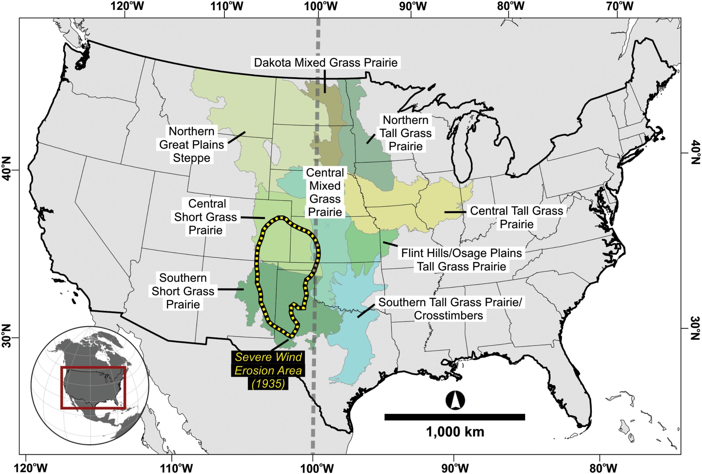
FIGURE 1. Location of the United States Great Plains delineated by terrestrial ecoregion (The Nature Conservancy [TNC] et al., 1995), with the 100th meridian demarcated by a dashed line and the classically recognized area of severe wind erosion at its maximum extent in 1935 (Worster, 1982; Cunfer, 2005).
There exists a large archive of pre-satellite panchromatic aerial photography for the conterminous United States that provides an unparalleled network of images for historical landscapes coincident with large-scale human modification characteristic of the 20th century (Redweik et al., 2009; Morgan et al., 2010; Nagarajan and Schenk, 2016). The USGP has a particularly rich photographic record beginning in the 1930s, when the United States Department of Agriculture was tasked with reducing acreage under cultivation to stabilize crop prices during the Great Depression (Leedy, 1948; Rango et al., 2008, 2011; National Archives and Record Administration[NARA], 2017). The resulting record, completed from 1935 to 1954, covers approximately 7,627,515 km2, or 99.5% of the contiguous United States (Leedy, 1948; National Archives and Record Administration[NARA], 2017) and is comparable in resolution to QuickBird and IKONOS satellite imagery (Laliberte et al., 2004; Rango et al., 2008; Browning et al., 2009). Recently a new historical image product was created from this record by applying advances in remote sensing and geospatial techniques to digital reproductions of original reel film (Bolles et al., 2017).
Previous studies using early aerial photographs are typically focused on changes in the distribution and cover of vegetation (cf. Carmel and Kadmon, 1998; Laliberte et al., 2004; Rango et al., 2008; Browning et al., 2009; Williamson et al., 2011; Morgan and Gergel, 2013; Murray et al., 2013; Lishawa et al., 2013). Bare surfaces are often filtered from analyses to increase accuracy of vegetation studies given the noise introduced to image classification schemes by soil spatial heterogeneity (O’Brien et al., 1982; Escadafal and Huete, 1992; Browning et al., 2009; Murray et al., 2013). However, heterogeneity is a significant concept in landscape ecology linked to ecosystem functioning, defined as the degree of spatial variability of a particular property within a scale-dependent system (Turner, 1989; Wiens, 1989; Li and Reynolds, 1995; Pickett and Cadenasso, 1995; Morgan and Gergel, 2010). Heterogeneity of bare soil surfaces is an indicator of landscape sensitivity to aridity, with increased patchiness frequently correlated with degradation (Schlesinger et al., 1990; Tongway and Ludwig, 1994; Bastin et al., 2002; Ravi et al., 2010; Bestelmeyer et al., 2011). Patch size, condition, and landscape context are significant factors in determining ecosystem resistance and resilience to climatic perturbations (Samson et al., 2004; Evans et al., 2011; Collins et al., 2014; Moran et al., 2014; Ruppert et al., 2015; Svejcar et al., 2015; Byrne et al., 2017). A framework for assessment of grassland degradation is defined by an index of the spatial distribution of land cover, coupled with an index of soil stability largely related to sediment texture and/or surface crusts (Tongway and Ludwig, 1994; Maestre et al., 2003). Utilizing semi-automated image analysis techniques, these metrics can be quantified for historic landscapes to examine biotic and abiotic controls on land cover changes (Browning et al., 2009; Morgan and Gergel, 2010, 2013; Morgan et al., 2010; Vogels et al., 2017). The resultant image products offer extended spatial scales to paleoarchives such as lake cores, stratigraphic sections, and tree-rings, and elucidate the interplay between climate, geomorphology, vegetation, and land use (e.g., Lishawa et al., 2013; Bolles et al., 2017; Schook et al., 2017).
There are well developed standards for manual interpretation of individual or stereoscopic pairs of aerial photographs with traditional photogrammetry. However, methods are emerging for semi-automated radiometric and spatial homogenization and structure-from-motion (SfM) photogrammetry for large numbers of archival black and white photographs (e.g., Morgan et al., 2010; Morgan and Gergel, 2013; Nebiker et al., 2014; Gonçalves, 2016; Bakker and Lane, 2017; Giordano et al., 2017; Mertes et al., 2017; Mölg and Bolch, 2017; Pacina and Popelka, 2017; Vogels et al., 2017; Sevara et al., 2018). Raw panchromatic aerial photographs are produced via black and white emulsions, where color is related to relative brightness of the visible light spectrum reflected from the surface (Caylor, 2000). When digitized, photographs are displayed as a single-band, gray-scale image, wherein each pixel is assigned a digital number (DN) that is proportional to the brightness of that pixel. Surface brightness is potentially altered by several parameters, not limited to viewing angle, azimuth and intensity of radiation source, sample geometry (i.e., particle size, aggregate size, roughness), vegetation cover, surface crusts, soil moisture and organic matter content (Escadafal and Huete, 1992; Ben-Dor, 2002; Mather and Koch, 2011). Particle size specifically can alter the shape of bare surface spectra by 5% of the absolute surface reflectance (Hunt and Salisbury, 1970; Ben-Dor, 2002). In field conditions aggregate size can be more significant than particle size and may change over sub-daily to monthly timeframes due to tillage, soil erosion, eolian accumulation, and/or crust formation. Therefore, surface roughness is an important determinant of the range of spectra expressed in aerial imagery (Ben-Dor, 2002; Zhang et al., 2003). These local factors are a challenge for analysis of aerial imagery, as manual interpretation of features can be subjective and labor-intensive to undertake over large areas and/or fine-scales (Morgan et al., 2010; Morgan and Gergel, 2013).
The principal characteristics available for feature identification in panchromatic imagery are variation and relative differences in tone (Morgan et al., 2010). Classification of tonal variation assigns individual pixels a label based on a specific property (Gennaretti et al., 2011), in this case the DN of each pixel. Relative differences in tone, also referred to as image texture, are determined by the spatial relationships between pixels within a defined area and directionality (Morgan and Gergel, 2010, 2013; Morgan et al., 2010; Vogels et al., 2017). Quantification of image texture can account for tonal heterogeneity and thereby, surface roughness (Morgan and Gergel, 2010), and is particularly useful for landform and land use classification where radiometric properties are being classified (Morgan et al., 2010). A significant assumption of this approach is that separate classes are represented by discrete differences between gray scale values and that these classes are spectrally independent (Anderson and Cobb, 2004). Where vegetation cover is only partial, a mixed signal from soil and vegetation occurs, making extrication of overlapping soil–vegetation signals complex (Ben-Dor, 2002), but this can be addressed via geographic object-based image analysis (GEOBIA; Morgan and Gergel, 2010, 2013; Blaschke et al., 2014; Vogels et al., 2017).
Herein, we present methods to analyze pre-1945 panchromatic aerial photographs along climatic gradients of USGP grasslands and evaluate landscape response to the 1930s Dust Bowl Drought (DBD). Specifically, we (1) identify representative study sites across various ecoregions of the USGP, (2) incorporate spectral, texture and object-based parameters to classify photo-mosaics and verify surface types of historic landscapes, and (3) quantify surficial heterogeneity and evaluate potential drivers of landscape response to drought. This research will examine the indicators and extent of landscape sensitivity to precipitation variability prior to widespread irrigation of the USGP and address controls on ecosystem degradation during severe drought years in the DBD.
Ecological and Geomorphic Factors for the United States Great Plains Landscape
Mean annual temperature (MAT) on the USGP is typically 15° to 18°C and mean annual precipitation (MAP) ranges from <250 mm in the west to >1,500 mm in the east, spanning the transition between semi-arid to sub-humid climates. The latitudinal zonation of northern to southern ecoregions generally follows temperature trends (Figure 2A); the short-to-tall grass prairie transition parallels the strong west-to-east MAP gradient (Figures 2B,C). Grassland ANPP is highly correlated to precipitation, with peak values of >700 g m-2 along the eastern margin of the Plains and decreasing to 80 g m-2 in the fore of the Rocky Mountains (Sala et al., 1988). On the USGP, terrestrial carbon storage may range from ∼0.3 to 0.9 kg C m-2 (Derner et al., 2006; Petrie et al., 2016), but can be a net atmosphere carbon source through diminished evapotranspiration and/or increased soil erosion (Meyers, 2001).
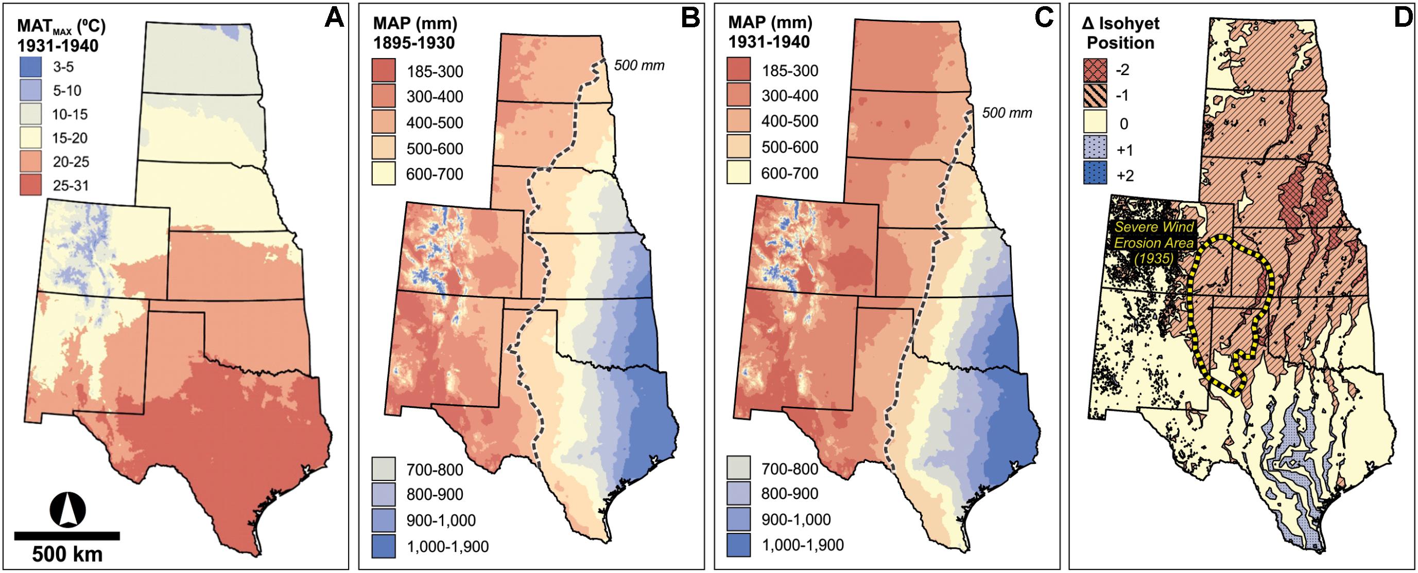
FIGURE 2. (A) The latitudinal gradient of northern to southern grasslands generally follows mean annual maximum temperature (MATMAX). (B) From 1895 to 1930 the position of the longitudinal mean annual precipitation (MAP) gradient generally corresponds to the short-to-tallgrass transition, but (C) during 1931 to 1940 MAP over the plains was significantly drier, and (D) this gradient was shifted eastward ∼250 km compared to MAP in the previous 36-year period, encompassing the largest extent of recognized severe wind erosion during the Dust Bowl (Worster, 1982; Cunfer, 2005). Temperature and precipitation data is derived from PRISM Historical Past time series datasets (PRISM Climate Group, Oregon State University, http://prism.oregonstate.edu, created October 3, 2017).
The USGP arid–humid divide roughly coincides with the 100th meridian, where precipitation decreases from ∼600 mm in the east to ∼400 mm in the west (Figure 2B) (Nielsen, 2018; Seager et al., 2018). This gradient shifted about 250 km eastward between 1931 and 1940 compared the prior MAP between 1895 and 1930, encompassing the largest extent of previously recognized severe wind erosion during the DBD (Figure 2D). Drought and land use directly impact grassland functioning via an increased risk of degradation, desertification, and subsequent reduction in stability and productivity, such as that observed during the DBD (Cook et al., 2009; Koerner and Collins, 2014; Ruppert et al., 2015; Lei et al., 2016; Byrne et al., 2017; Hu et al., 2018). However, the DBD was not a homogeneous event in time or space but consisted of several droughts and relative wet phases affecting different regions at different times (Figure 3) (Laird et al., 1998). Drought conditions were exacerbated by above-average temperatures exceeding 40°C and land–atmosphere interactions that increased the threshold for precipitable water (Cook et al., 2011a,b, 2014; Su et al., 2014; Donat et al., 2016). Climate modeling studies of the DBD have found that land cover changes increased the intensity and altered the spatial footprint of drought across the USGP (cf. Cook et al., 2008, 2009; Hu et al., 2018).
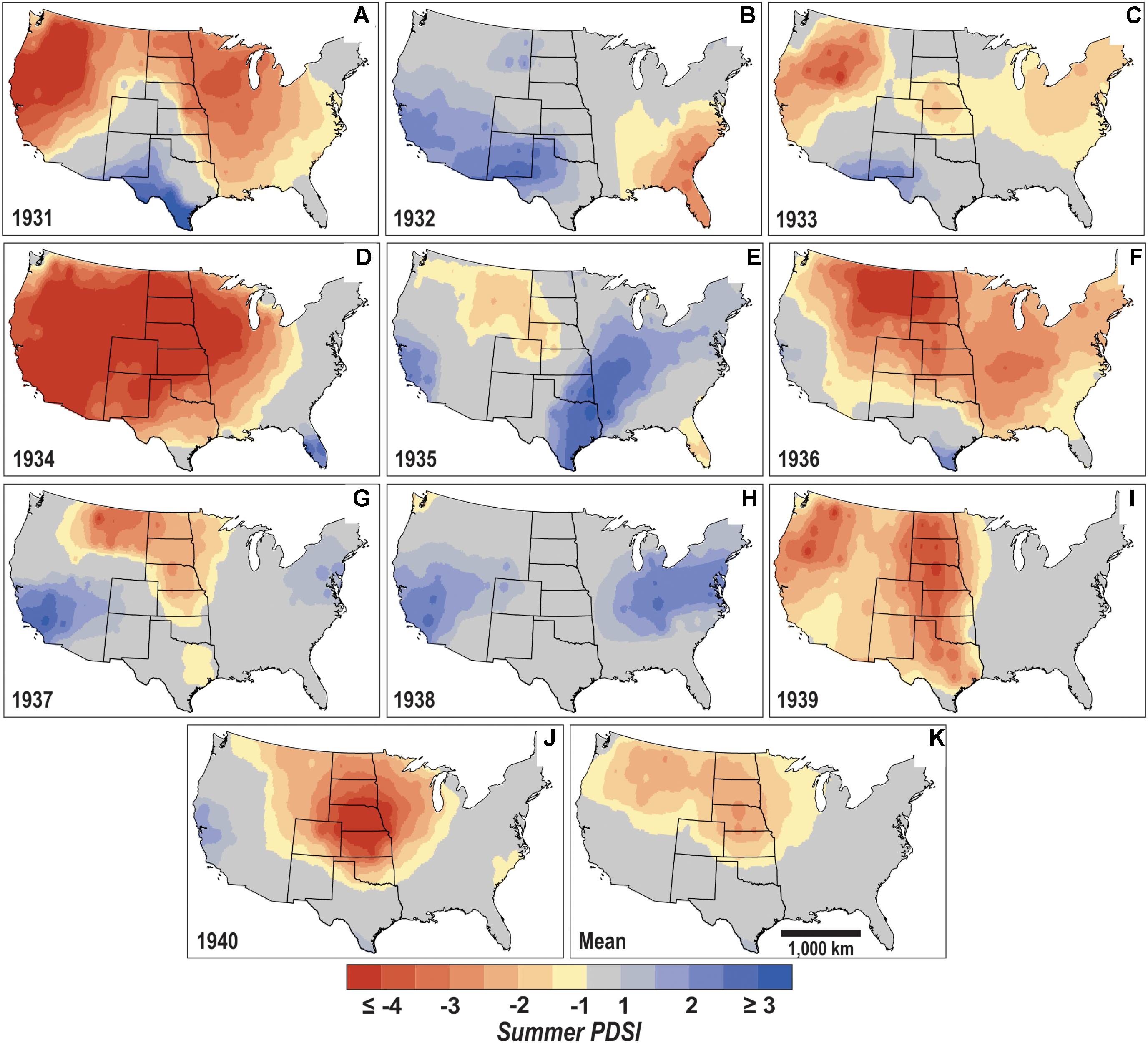
FIGURE 3. (A–K) Summer (June–August) Palmer Drought Severity Index (PDSI) for the years 1931–1940 and the decadal mean calculated from the North American Drought Atlas (Cook et al., 2010).
Reduced vegetation cover allows for enhanced wind erosion of soils, burying of adjacent grasses by the accumulation of eolian sediment and an increase in overland flow and riling from episodic and extreme rainfall events (Schlesinger et al., 1990). The subsequent recovery of plant communities may be delayed a decade or more, even with 5 years of precipitation above the historical average, as observed after the DBD (Weaver and Albertson, 1956, pp. 128–162). Ecological studies in the 20th century indicated that the diversity of grassland species decreased with drought, excessive grazing, and range fire (Albertson and Weaver, 1944; Tilman and Downing, 1994; Collins et al., 1998). The climax grassland species, such as Blue Grama (Bouteloua gracilis) and Buffalo Grass (Buchloe dactyloides), have decreased vitality with drought because of a shallow root system (<1 m). As drought persists for grasslands, the surficial heterogeneity increases with the dominance of bare surfaces with biomass and nutrients focused by deeply rooted (2–5 m) woody vegetation, forming “islands of fertility” (Weaver and Albertson, 1943, 1956, pp. 86–116; Schlesinger et al., 1990; Jurena and Archer, 2003).
In semi-arid regions such as the USGP, there are also apparent responses in eolian and fluvial geomorphic systems to extreme precipitation variability (Ewing et al., 2006; Derickson et al., 2008; Ewing and Kocurek, 2010; Ravi et al., 2010; Turnbull et al., 2010; Belnap et al., 2011; Liu and Coulthard, 2015). The pattern of stabilized dunes is often linked to bioclimatic variations. Wetter spring and summer conditions and heavy winter snowfall provide excess moisture for eolian systems to stabilize more effectively, with colonization by climax vegetation assemblages (Cordova et al., 2005; Ravi et al., 2010; Turnbull et al., 2010). Drier conditions are often correlated with decreased vegetation coverage and increased eolian activity, such as during the Medieval Climate Anomaly (MCA) when multiple, multi-decadal droughts propagated across the Americas with numerous presently stabilized eolian sand systems apparently reactivated, but to an unknown spatial extent (e.g., Mason et al., 2004; Forman et al., 2005, 2008; Lepper and Scott, 2005; Seifert et al., 2009; Halfen and Johnson, 2013). Many periods of eolian reactivation exhibit discontinuous blow-outs, parabolic dunes and sandsheet accretion, often leaving a spatially heterogeneous landform assemblage (Schlesinger et al., 1990; Hugenholtz and Wolfe, 2005, 2006). Questions remain if such degradation is in response to landscape-scale drier conditions, or if soil erosion is a stochastic process reflecting randomness or localized surficial disturbance of vegetation with drought, grazing, fire and/or pestilence (e.g., Schlesinger et al., 1990; Bel and Ashkenazy, 2014).
Materials and Methods
A standardized workflow (Figure 4) was developed to select, process, analyze, and archive aerial photographs captured between AD 1936 and 1941 from counties across the USGP based on previously defined iterative analyses (Okeke and Karnieli, 2006; Redweik et al., 2009; Morgan et al., 2010; Morgan and Gergel, 2013; Doneus et al., 2016; Gonçalves, 2016; Bolles et al., 2017; Vogels et al., 2017). In brief, photogrammetric scans of original reel film are corrected for interior and exterior distortions of position and light exposure. Processed frames are spatially referenced to the North American Datum 1983, Universal Transverse Mercator, Zone 14N (NAD83 UTM 14N), with a residual root mean square error (RMSE) ≤ 5 m. Frames are then resampled to a standard resolution (1 pixel = 0.25 m2) and blended into a mosaic based on county location and date of negative acquisition. Surface properties are retrospectively verified using historical primary documentation, contemporary field surveys, and digital surface models (DSMs) derived with SfM photogrammetry, allowing for assessment of uncertainty of manual and automated classifications. Spectral analysis of individual pixels, texture analysis of multiple pixels within a sliding window (i.e., a texel), and subsequent segmentation of groups of pixels into objects are applied to mosaics. Image and verified data are combined to classify objects based on surficial properties, including soil texture, land cover, land use, and geomorphic form, and classification results are statistically analyzed. The number of surface types accounting for ≥50% and ≥90% of a respective study area are used to define thresholds in surficial diversity.
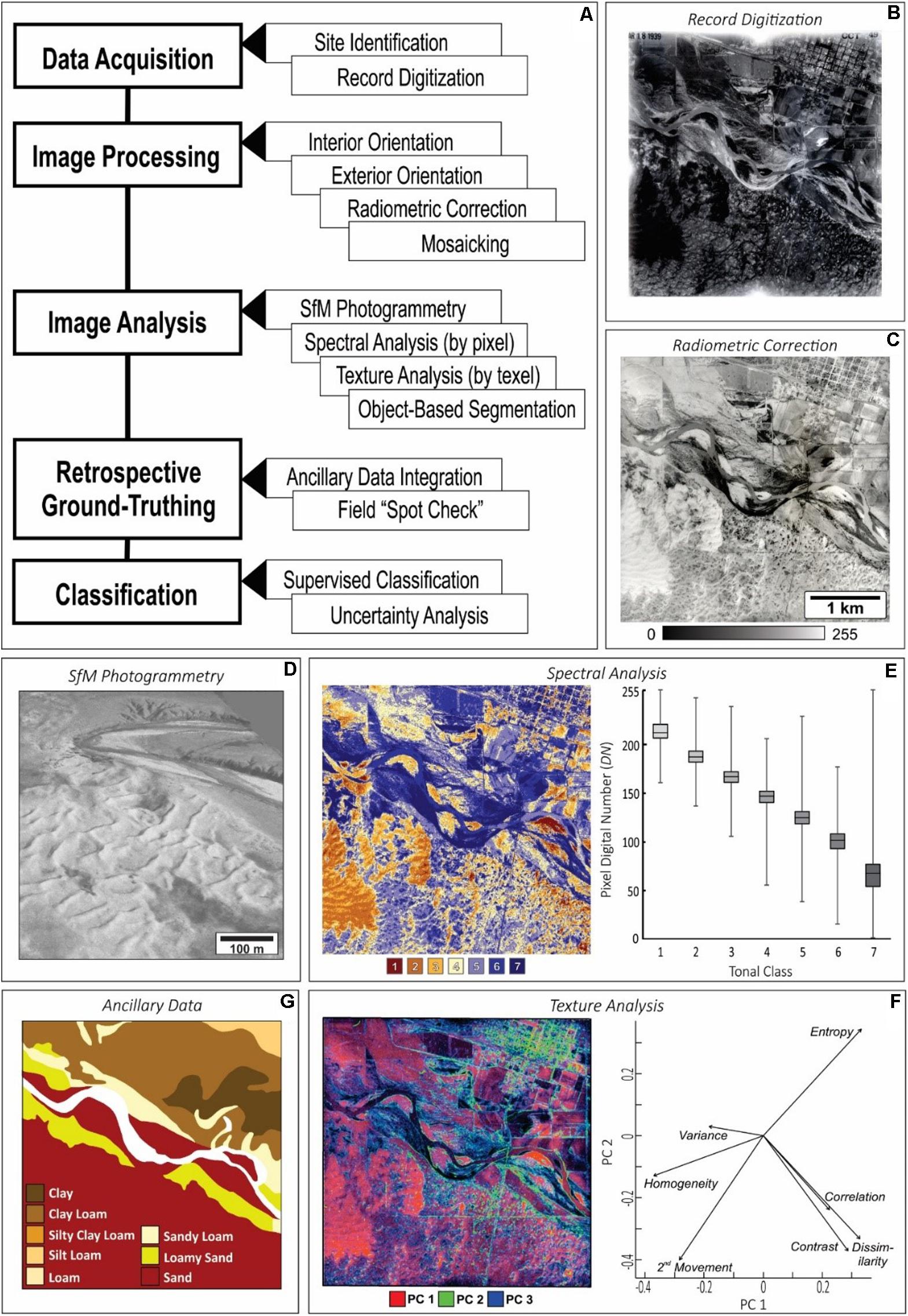
FIGURE 4. Outline of semi-automated analysis of historical panchromatic aerial photographs used in this study with illustrative example: (A) diagrammatic workflow of methods used, (B) raw scan of original negative reel film of frame 145-CCT-049-155 from Syracuse, Hamilton County, KS taken March 22, 1939, (C) oriented, radiometrically corrected, and resampled image, (D) digital surface model (DSM) generated from multi-view stereoscopy, (E) results of unsupervised spectral classification of pixel digital numbers (DN) with box and whisker plot of cluster distribution, where the gray-scale color of the box in the plot corresponds to the mean DN of the cluster; refer to Table 4 for legend description, (F) results of principal component analysis of image texture layers to delineate image objects, (G) soil surface texture gathered from the Web Soil Survey (Soil Survey Staff [SSS] et al., 2017).
Study Site Identification and Photograph Reproduction
A multi-criterion, spatially explicit weighted overlay is employed to identify USGP counties that are representative of the broader landscape for the time and place of negative acquisition and to minimize subjectivity in site selection (Table 1). We include three climatic parameters to estimate the magnitude of anomalies in each county between 1931 and 1940, with larger deficits given greater weight: percent change in maximum MAT and MAP relative to the preceding 35-year period (1895–1930), and the central tendency of evapotranspiration as expressed by the mid-range Palmer Drought Severity Index (PDSIMR; Figures 5A–C). Three physical surficial parameters averaged at the county level were included to evaluate the similarity of landscape setting amongst counties within the same ecoregion, with values closest to the regional mean weighted highest: sediment texture (% sand, silt, and clay in upper 20 cm of soil), density of fluvial drainages expressed as a ratio of total channel length to county area, and percent area under cultivation per the Agricultural Census of 1935, identified in historical analyses as the year of maximal cropland extent on the USGP (Cunfer, 2005; Figures 5D–F). These criteria are standardized to a scale of 1–9 and given equal influence in an overlay to assign each county a final rating that reflects the intensity of drought conditions and similitude of surficial properties to the broader ecoregion (Figure 5G). A fishnet of 1,000 km2 cells is created across counties within USGP ecoregions, and a random sample of cells distributed across the precipitation and temperature gradients is selected for acquisition of aerial photographs.
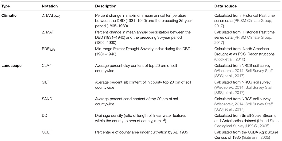
TABLE 1. Criteria included in the weighted overlay for site identification (with Figure 5).
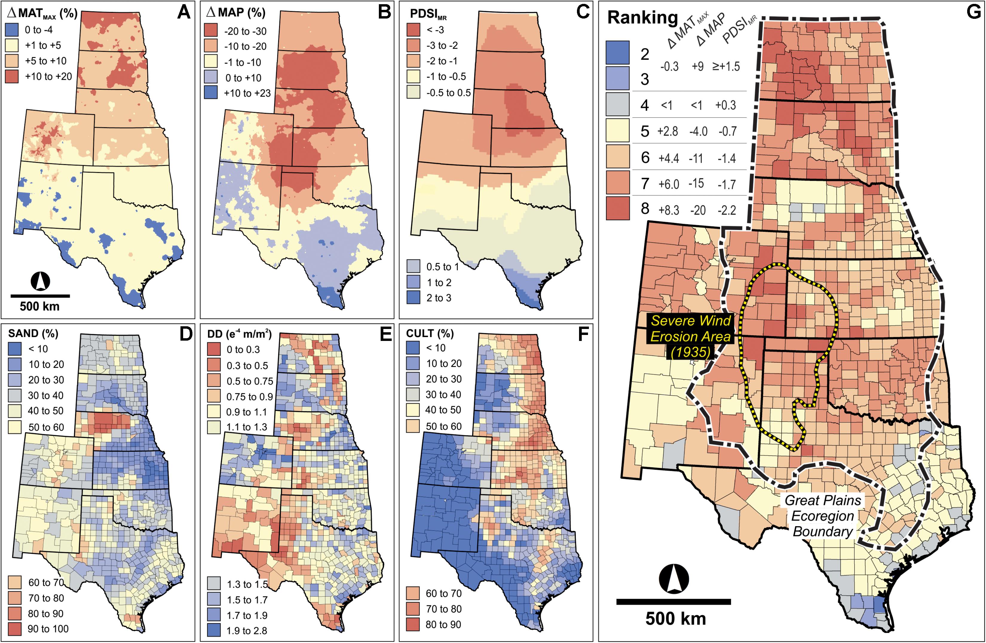
FIGURE 5. Layers included in the multi-criterion site selection scheme, including climatic factors (A–C) and surficial properties aggregated at the county-level (D–F): (A) percent change in mean annual maximum temperature (MATMAX) during 1931–1940 in comparison to preceding 35-year period (1895–1930), (B) percent change in mean annual precipitation (MAP) during 1931–1940 in comparison to preceding 35-year period, (C) mid-range Palmer Drought Severity Index (PDSIMR) during 1931–1940, (D) average percent sand, silt, and clay content of soil, (E) average drainage density (DD) expressed as a ratio of total length of linear water features to county area, and (F) the percent of acreage under cultivation at the peak of agricultural expansion in 1935. (G) Criteria were standardized to a scale of 1–9 and given equal influence in a weighted overlay to assign each county a rating based on its respective properties. For data sources, refer to Table 1.
Access to the primary photo archive is through the National Archives and Record Administration[NARA] (2017) II facility in College Park, MD, United States, where much of early aerial imagery has been centralized, with limited holdings at smaller archives (Rango et al., 2008; Sylvester and Rupley, 2012). At the facility, photograph reproductions are available as hardcopy photomosaics of the original flight lines, organized by record group, state, county, and year. Once the appropriate survey symbol, flight line and photo number associated with an area of interest are identified, the specific canister of original reel film, typically held at off-site cold storage, is ordered to NARA for digitization by a vendor with approved scanning equipment. The original scans used in this study are archived by county and available from the Historical Air Photo Dataverse at the Texas Data Repository (Bolles, 2018a–i). A subset of 657 high resolution (≥1,200 dpi) photogrammetric scans of overlapping negatives from six counties is utilized in this study (Table 2 and Figure 6). These images were taken at 1:20,000 scale between November 1936 and November 1940, with 35% lateral overlap between images and forward overlap from ∼35 to 67%.
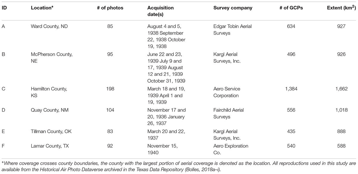
TABLE 2. Survey details and spatial extent of photos reproduced for this study from United States Department of Agriculture contracted surveys (with Figure 6).
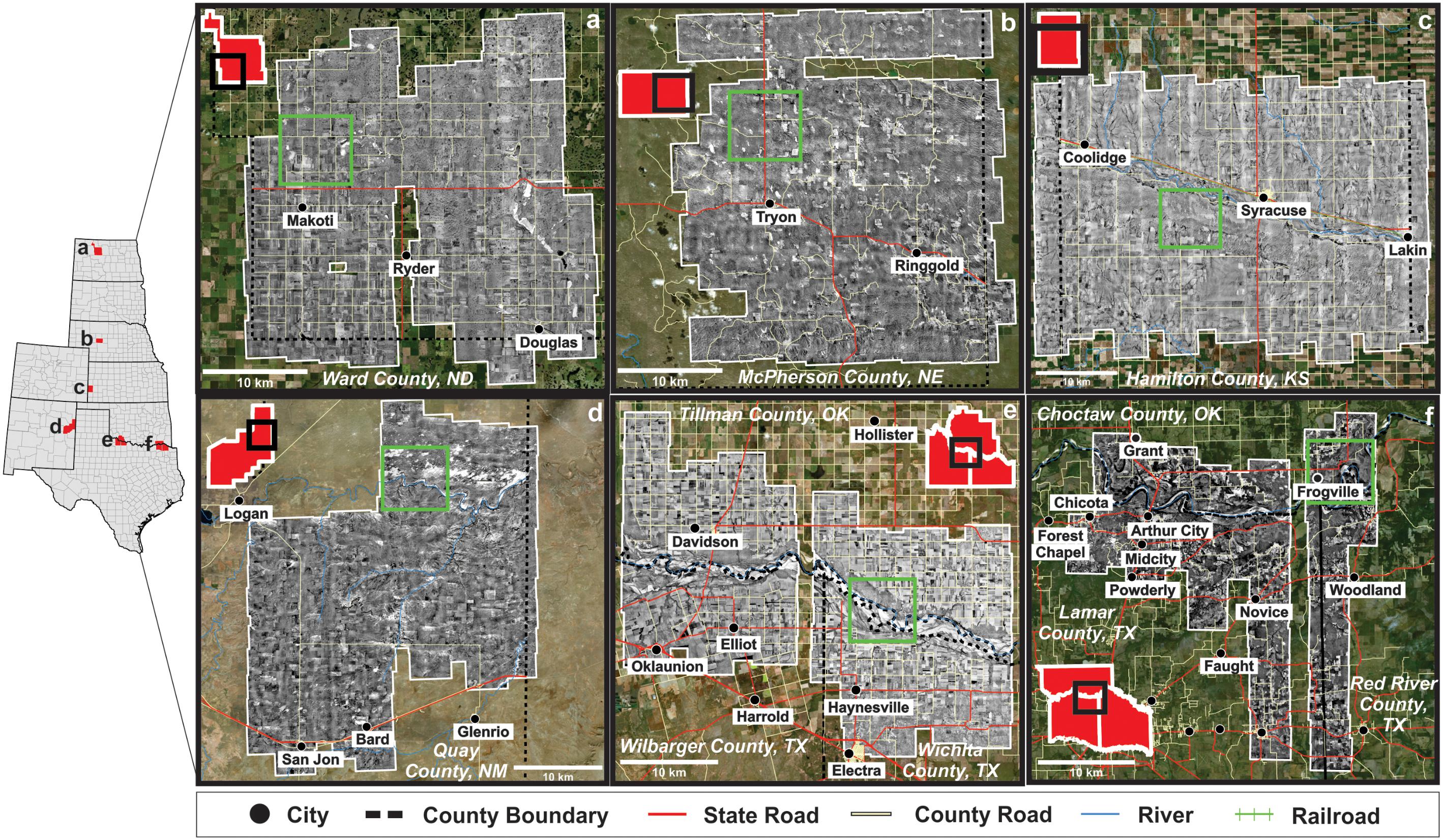
FIGURE 6. Location map of selected areas showing county position on the Great Plains and extent of aerial photographic coverage reproduced for this study in: (a) Ward County, ND, (b) McPherson County, NE, (c) Hamilton County, KS, (d) Quay County, NM, (e) Tillman County, OK, Wilbarger and Wichita Counties, TX, and (f) Choctaw County, OK, Lamar and Red River Counties, TX. Survey details for the mosaics are presented in Table 2. The green box denotes location of imagery shown in Figure 7.
Processing and Analysis of Digitized Historical Imagery
In lieu of coeval camera calibration reports, which are largely unavailable, the interior orientation of digitized images is corrected to pseudo-calibrated fiducial coordinates from a template image frame via an affine transformation in MATLAB (Leedy, 1948; Redweik et al., 2009; Gonçalves, 2016; Nagarajan and Schenk, 2016; Giordano et al., 2017). Images are then cropped to standard dimensions to remove outlying pixels from the frame, such as those obscured by the photograph collar and identification numbers (Heipke, 1997; Redweik et al., 2009; Doneus et al., 2016). Ground controls points (GCPs) are identified to correct for exterior orientation between image and coordinate space. Absent detailed flight logs containing roll, pitch, yaw, and position coordinates, GCPs are obtained by matching time-invariant features (TIFs) within the image to features in contemporary imagery with a known location (Nagarajan and Schenk, 2016). The base map within ERSI ArcGIS and vector data of roads from state GIS data repositories are used to derive 5–20 GCPs per frame to attain an RMSE ≤ 5 m.
Color correction is concentrated on contrast enhancement to distinguish the intergrades in brightness from bare to fully vegetated surfaces, and between the textural properties of those surfaces (Kadmon and Harari-Kremer, 1999; Murray et al., 2013; Liu and Mason, 2016). The open-source, python-based GNU Image Manipulation Program (GIMP) is utilized to normalize the histogram of each frame individually, then to gamma-balance across frames so overlapping features are displayed along the same radiometric range (Kadmon and Harari-Kremer, 1999; Murray et al., 2013). Images are monochromatically balanced to correct for light fall-off introduced by lens distortion, spatially variable characteristics of the original film, and/or improper exposure of the photograph (Figures 4B,C; Redecker, 2008; Morgan et al., 2010). Frames are then further color balanced in an ESRI ArcGIS mosaic dataset using a first-order smoothing algorithm to minimize merging of pixels that do not match. Frames are blended together along seamlines generated from spectral patterns of overlapping features; the frames with greatest spatial accuracy (i.e., lowest RMSE) are weighted forward in seamline delineation and blending.
Multi-view stereoscopy of overlapping aerial photography is a rapidly developing method for landscape-level analyses of historical surfaces (Gomez, 2012; Nebiker et al., 2014; Doneus et al., 2016; Mertes et al., 2017; Mölg and Bolch, 2017; Pacina and Popelka, 2017; Sevara et al., 2018). The Agisoft Photoscan (APS) software package is used for automated three-dimensional reconstruction of the surface; the APS algorithm generates dense point clouds on par with airborne LiDAR data to derive a triangulated surface representing a DSM (Figure 4D) (Nebiker et al., 2014; Pacina and Popelka, 2017). Subsequently the DSM is used to calculate slope and elevation as covariate parameters for image classification. The centroid coordinates of each frame footprint created in the mosaic dataset is utilized to approximate the camera position at the time of acquisition to increase accuracy in photogrammetric alignment within APS.
The Iterative Self-Organizing Data Analysis (ISODATA) classification in ESRI ArcGIS is a robust clustering algorithm for areas with sparse ground-truth data and is used initially to understand the distribution of pixels DNs within a mosaic (Ball and Hall, 1967; Liu and Mason, 2016). An exaggerated number of clusters (≥15) is established across the range of spectral values, and neighboring clusters are merged until the overlap between cluster quartiles is ≤1% (Figure 4E) (Anderson and Cobb, 2004; Skirvin et al., 2004; Okeke and Karnieli, 2006; Bolles et al., 2017). A majority filter is applied to reclassify pixels where it can be reasonably assumed the pixel belongs to the surrounding cluster, producing a smoothing effect (Mather and Koch, 2011; Liu and Mason, 2016). Whereas this is a powerful tool to assess vegetation cover and soil texture, distinctions in land use and geomorphic form are often obscured. For example, an unpaved road, eroding field, and migrating dune are clustered together given similarities in surficial brightness. Thus, more information about patterns between adjacent pixels is needed to classify surficial processes and land use.
Using a MATLAB script, we calculate gray-level co-occurrence matrices for several textural properties within a 3 × 3 moving window (Haralick et al., 1973; Laliberte et al., 2004; Morgan and Gergel, 2010, 2013; Morgan et al., 2010; Mather and Koch, 2011; Schowengerdt, 2012; Vogels et al., 2017). This returns the probabilities of occurrence of a specific pixel pairing in eight directions, the average of which is taken to define the final texture parameter for each texel (i.e., the block of pixels within the moving window). The resulting texture rasters are used as inputs for principal component analysis (PCA) to identify statistically significant relationships between texture parameters and group pixels for object-based image segmentation (Figure 4F). Segmented objects are overlaid with the DSM to categorize landform and land use, then combined with surficial soil texture and tonal class to obtain the final classification of unique surface types (cf. Morgan and Gergel, 2010, 2013; Blaschke et al., 2014; Parajuli et al., 2014; Baddock et al., 2016; Parajuli and Zender, 2017; Vogels et al., 2017).
Retrospective Land Surface Verification
There is a wealth of observations on land surface conditions during the 1930s that has previously provided the basis for environmental interpretations (Browning et al., 2009; Skaggs et al., 2011; Williamson et al., 2011). Data sources are from contemporaneous peer-reviewed publications, government records from the Soil Conservation Service (SCS), ancillary experiment stations, and ground-based photographs held at NARA II facility in College Park, MD, United States. Items reviewed and digitized include: handwritten field notes, field photographs, planimetric maps, documentation of tillage operations, and correspondence between land owners, scientists and government officials. A complementary data source is the study of near-surface eolian deposits and landforms that are associated with landscape degradation during the DBD (e.g., Forman et al., 2008; Bolles et al., 2017). Specifically, the dry Munsell Color of bare sand and buried soils is a useful corollary to connect image grayscale and soil texture. This index designates the hue, chroma, and value of a given material, where value (or brightness) is the first parameter established and ranges in equal intervals from black to white. The Web Soil Survey from the National Resource Conservation Service (NRCS; Soil Survey Staff [SSS] et al., 2017) is also used to delineate the lateral variability in soil texture. Finally, an Abrams stereoscope is used with hardcopy image stereo-pairs to randomly “spot check” the sense of slope and elevation measurements taken from the DSMs.
Statistical Analyses
Bivariate and multivariate statistical approaches are applied to parse the potential relationships between a matrix of 52 variables measured from the six study sites. Variables include criteria from the site selection scheme (Table 3), classified land surface parameters (Table 4), and summer PDSI from 1931 to 1940 interpolated from the North American Drought Atlas (Figure 3) (Cook et al., 2010). Data are standardized, and a comparison of skewness and standard error values indicates about half of variables measured are not normally distributed. Therefore, Spearman’s rank correlation coefficient (RS) is calculated to explore the strength and direction of dependence between the rank order of variable pairs (Borradaile, 2003). Pairs with an RS over ±0.8 and a p-value ≤0.05 are considered as significant variables with a strong monotonic relation. A PCA of the same matrix reveals linear combinations of variables with the maximum amount of covariance, and the subsequent principal components (PCs) are mutually uncorrelated (Wilks, 2011). A threshold is applied to extract coefficients in the upper or lower quintile of PC eigenvalues and identify the dominant variables contributing to intra- and inter-site variance. Finally, two pairwise distance metrics are computed between sites to create hierarchical cluster trees (Wilks, 2011): cosine (one minus the cosine of the angle between points) and hamming (percentage of coordinates that differ).
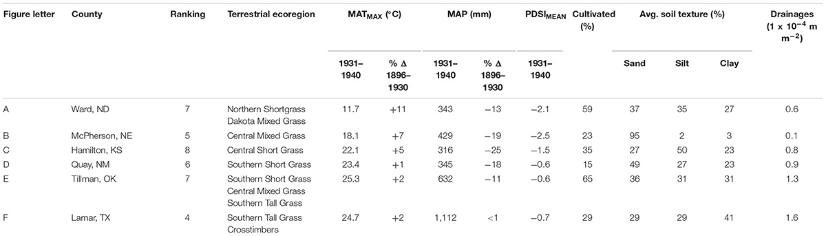
TABLE 3. Climatic conditions and landscape setting for the six study areas during the 1930s Dust Bowl Drought with county ranking and criteria from the site selection scheme (Table 1 and Figure 5).
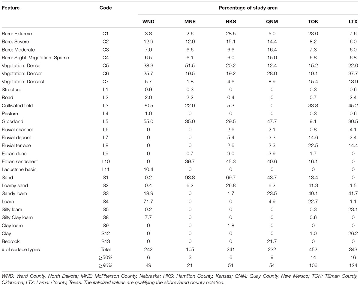
TABLE 4. Distribution of quantified landscape variables across the six study counties, number of unique surface types classified, and number of surface types accounting for at least 50% and 90% of the study area.
Results
Great Plains counties during the 1930s exhibit a range of inferred drought conditions and degree of similarity in antecedent landscape setting to the broader region, from a ranking of 4, associated with moderately mesic conditions, to a score of 8 indicating severe drought areas (Figure 5G). The counties rated ≤4 display relatively neutral conditions over the decade and are largely located near the Texas coast. Whereas those counties rated 5 or higher are associated with increasing intensity of drought conditions on the USGP. Counties rated 5 or 6 are largely evenly distributed across the short- to tallgrass transition but show a slight increase in frequency east of the 100th meridian. The majority of counties ranked 7 contain shortgrass species (52%), most frequently located in the central shortgrass prairie ecoregion. Forty-six counties (6%) receive the highest rank of 8, characterized by PDSIMR of less than -2, maximum temperatures 5–10% higher than normal, and ≥20% deficit in precipitation. Of these counties, >70% are west of the 100th meridian in shortgrass ecoregions, most frequently Northern Great Plains Steppe.
The surface processes are discussed for six cells from across the USGP fishnet; note that if a cell crosses county boundaries, the county with the largest portion of aerial coverage is denoted as the location. The subset of counties selected for this study are: Ward, ND, McPherson, NE, Hamilton, KS, Quay, NM, Tillman, OK, and Lamar, TX. These counties reflect mild-to-severe DBD conditions and generally contain surficial properties typical of the respective ecoregion (Table 3). Across these six counties, seven clusters are derived from the spectral classification, and these tonal classes are indicative of vegetation cover and/or soil texture and moisture. This treatment includes the relative density of plant cover and general species assemblage from historical documentation, a scheme modified from Bolles et al. (2017). Broadly, 34% of the 652 unique surface types are classified as denuded, with the remaining 66% covered by natural vegetation or crops, though this ratio, type of vegetative cover, and loci of degradation fluctuate across ecoregions (Tables 4, 5 and Figure 7).
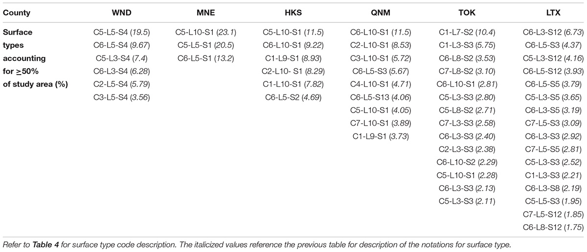
TABLE 5. Surface types covering at least 50% of the respective study area.
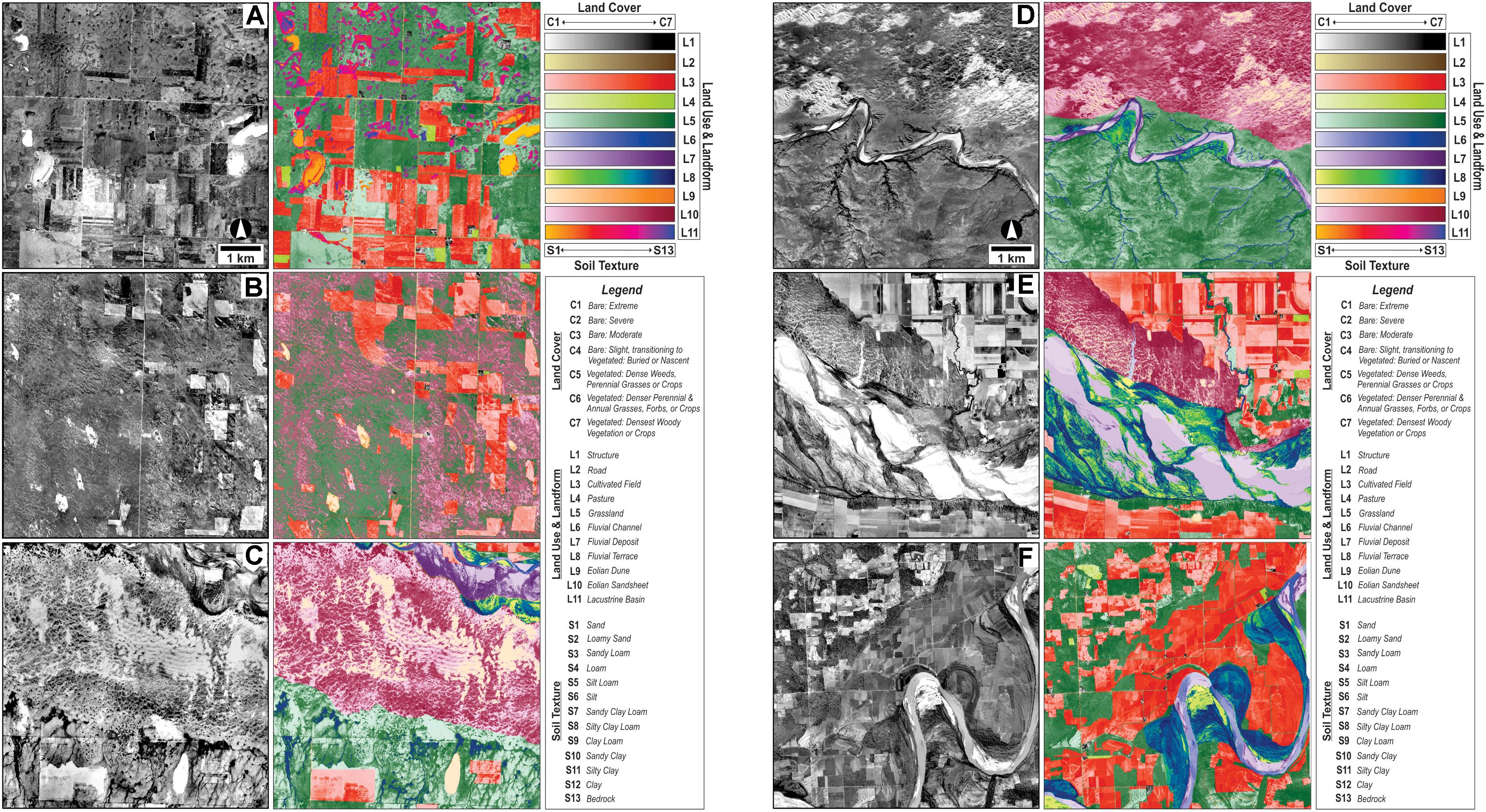
FIGURE 7. Illustrative samples from image analysis and classification from processed aerial photographs of (A) Ward County, ND, (B) McPherson County, NE, (C) Hamilton County, KS, (D) Quay County, NM, (E) Tillman County, OK, Wilbarger and Wichita Counties, TX, and (F) Choctaw County, OK, Lamar and Red River Counties, TX. Refer to the corresponding letter in Figure 6 for location denoted by a green box. Column one is an enhanced view of ∼45 km2 from the blended mosaic; column two presents the final supervised image classification of landscape features.
Ward County, North Dakota
Ward County, ND (Figure 7A) occurs at the transition from northern mixed-grass prairie to steppe vegetation and by 1935 was ∼60% cultivated. This county ranked 7, experiencing maximum temperatures 11% higher in the 1930s than in the prior three decades, and with a 13% precipitation deficit. At the time of negative acquisition in the fall of 1938, most of the study area (∼70%) is an uncultivated mix of grasslands over alluvial floodplains and lacustrine basins, with 71% vegetation cover irrespective of land use or landform. Nearly 40% of uncultivated areas with plant cover are classified as patchy weeds and grasses, 25% as denser grasses and forbs, and ∼5% as woody vegetation. Cultivated fields appear mostly vegetated (73%) with severe cover loss when bare. Of the most extreme denudation, 80% is associated with natural landforms, at least half of which are identified as dried-out lake beds exposing silty clay loam. Nearly all lacustrine basins lack standing water; by 1939 total lake surface area was about one-third of the recorded high from 1868 to 1877 (Shapley et al., 2005). In total, 242 surface types are identified, with over half the study area described by six types (Table 5). The most common surface type is grassland dominated by weeds and perennial grasses colonizing loamy soils developed on glacial till.
McPherson County, Nebraska
McPherson County, NE (Figure 7B), ranked 5, falls within the central mixed-grass prairie ecoregion, was 23% cultivated by 1935, and during the DBD experienced a 7% increase in maximum temperatures and a 19% deficit in precipitation. The soils in this county, at the margin of the Nebraska Sand Hills, are characterized by ≥90% sand content (Figure 5D). The earliest available aerial photographic coverage for this county was July 1939, with 22% of the surface in cropland, ∼40% uncultivated undulating sandsheets and 35% interdunal grassland. Nearly three-quarters of the surveyed area (74%) is vegetated, though severe vegetation loss is frequently mapped in cultivated fields. Surfaces classified with the greatest degradation occur 64% on cultivated fields and 31% on blowout dunes, nascent parabolic dunes, and sandsheets. The crests of sandsheet ridges are most frequently disturbed. Blowouts are trough-shaped, sometimes reaching 0.5 km in length along the dominant axis, oriented NNW/SSE. In total, 105 surface types are identified, with >50% of the study area described by three classes (Table 5). This area is ∼23% vegetated sandsheet, and nearly equally common are patchy-to-dense weeds, grasses, and forbs in interdunal grasslands.
Hamilton County, Kansas
Hamilton County, KS (Figure 7C) yielded a ranking of 8, and experienced significant drought conditions during the DBD, with 5% higher maximum temperatures and an extreme precipitation deficit (-25%). Shortgrass prairie dominates this county, with largely sandy soils and smaller areas of clay loam soils. In 1935, agricultural census data indicates that 35% of the county was under cultivation, though only ∼5% is observed as actively tilled in the 1939 imagery used for this study, suggestive of farmland abandonment. Much of the vegetation present are grasses on alluvial surfaces and sparse cover on sandsheets, with the densest vegetation along fluvial channels. However, nearly half of the study area is devoid of vegetation at the time of negative acquisition. Almost 33% of bare areas are severely denuded with the presence of barchanoid-type ridges palimpsest with sand sheet deposits and occasional large blowouts (∼1 km). Slight-to-severe degradation is typically associated with sandsheets, nascent barchan dunes, and devegetated alluvial floodplains. Approximately 25% of cultivated surfaces are eroded, with sand apparently saltating across the landscape from the northern edges of fields. Cultivated fields and pastures exhibiting degradation are most often associated with loamy sand or clay loam soils, whereas nearly all bare uncultivated landforms are composed of sand or silty sand. In total, 241 surface types are identified, with over half the study area described by six classes (Table 5). Most common in this study area is vegetated sandsheet on sandy soil, followed by active sand dunes, and severely-to-extremely denuded sandsheet surfaces.
Quay County, New Mexico
The southern shortgrass prairie of Quay County, NM (Figure 7D) experienced slightly warmer maximum temperatures than previous decades but a large precipitation deficit during the DBD and is ranked a 6 in the site selection scheme (Table 3). A maximum of 15% of the county was under cultivation in 1935, and few cultivated surfaces are observed in the 1936 photographs analyzed in this study. Forty-five percent of the study area is bare; where vegetation is present, it is typically grasses and shrubs. Extreme degradation is largely associated with sand dunes (>75%) which most frequently are parabolic or partially reactivated barchanoid ridges, oriented NE–SW. Severe degradation is also observed for some fluvial surfaces, such as point bars and tributaries of the Canadian River, and sheet and rill erosion above incised channels. In total, 232 surface types are identified, with over half the study area described by nine classes (Table 5). The largest proportion of the study area is mapped as vegetated sandsheets developed on antecedent eolian sands, followed by severely degraded sandsheets.
Tillman County, Oklahoma
Tillman County, OK (Figure 7E) falls at the confluence of the three dominant ecoregions of the Great Plains: short-, mixed-, and tallgrass prairie. This county, rated 7, experienced an 2% increase in maximum temperatures and 11% precipitation deficit during the DBD, and in spring of 1937 exhibited ∼40% bare surfaces. Vegetated surfaces are evenly distributed across grasses, woody vegetation, and cropland. Cultivated surfaces are frequent; over half of fields are bare, with 25–30% classified as severely denuded. However, of the unvegetated areas ∼60% is associated with fluvial deposits in the main channel and tributaries of the Red River, with dunes superimposed on terraces and partially active, reflecting a complex interaction between eolian and fluvial geomorphology and potentially influencing the evolution of both features (Liu and Coulthard, 2017). The majority of moderate-to-severe degradation occurs on cultivated fields, with the remainder common to older, topographically higher fluvial terraces with active sandsheets. This county exhibits a marked increase in diversity of soil type, land use and landforms than those counties west of the 500 mm precipitation isohyet. In total, 452 surface types are identified, with over half the study area described by 14 classes (Table 5). The greatest portion of denuded area is mapped as bare fluvial deposits of loamy sand, followed by cultivated fields with sandy loam soils.
Lamar County, Texas
Lamar County, TX (Figure 7F) covers the transition between southern tallgrass prairie to crosstimbers ecoregion and experienced largely neutral conditions during the DBD, receiving a rating of four. Approximately 45% of the study area is classified as cultivated fields and ∼50% associated with the fluvial landforms and floodplain of the Red River. Less than 30% of the surveyed area is bare, and a robust population of woody vegetation colonizes uncultivated surfaces. Generally dense vegetation is absent where land was cleared for cultivation. The majority (50–60%) of bare surfaces occurs in cultivated fields, and many fields relict show nebkha dunes, ∼10 to 25 m in diameter and up to 2 m in relief (cf. Seifert et al., 2009). Among natural surfaces, deposits within the active channel of the Red River lack plant cover. Much of the moderate-to-severe degradation is associated with gullies on older fluvial terraces, whereas incipient vegetation loss is most frequently observed across the active floodplain. In total, 343 surface types are identified, with over half the study area described by sixteen classes (Table 5). The largest percentage of the study area is mapped as vegetated cultivated fields on clay soils, and dense vegetation on uncultivated loamy sand, silt loam, and clay soils.
Correlations, Components, and Clusters of Ecoregion Variance
A statistical analysis was undertaken to evaluate the relation amongst land cover classes, landscape attributes and climatic variables. The extent of extremely denuded surfaces is positively correlated to loamy sand soils and fluvial deposits (e.g., point bars, alluvial islands; Figure 8A). Areas of severely denuded surfaces are negatively monotonic with silty loam soils, cultivated fields, and MAP (Figure 8B). Patchy cover of weeds and grasses increases where the summer PDSI of 1932, 1937, and the mean PDSI from 1931 to 1940 are lower (Figure 8C). Dense, woody vegetation coverage increases with area of sandy loam soils, the density of fluvial drainages, the mid-range PDSI value during the DBD, and the number of surface types explaining at least 50% of site surficial diversity (Figure 8D). The association between woody vegetation and greater diversity of surface types is further reinforced by shared monotonic trends with the summer PDSI for 1934 and 1935 (RS = 0.943, p = 0.017), the change in maximum MAT (RS = -0.841, p = 0.044), the average percentage of clay in county soils (RS = 0.886, p = 0.033), and dominant ecoregion (RS = 0.882, p = 0.033). The total count of surface types classified is positively correlated with area of silty loam soils (RS = 0.88, p = 0.05) and the proportion of area under cultivation by 1935 (RS = 0.886, p = 0.033). There is a positive correlation between areas of silty loam soils and cultivated fields (RS = 0.941, p = 0.017). Cultivated fields are negatively correlated with sandsheets (RS = -0.841, p = 0.044), though sandsheets trend positively with active dunes (RS = 0.941, p = 0.022).
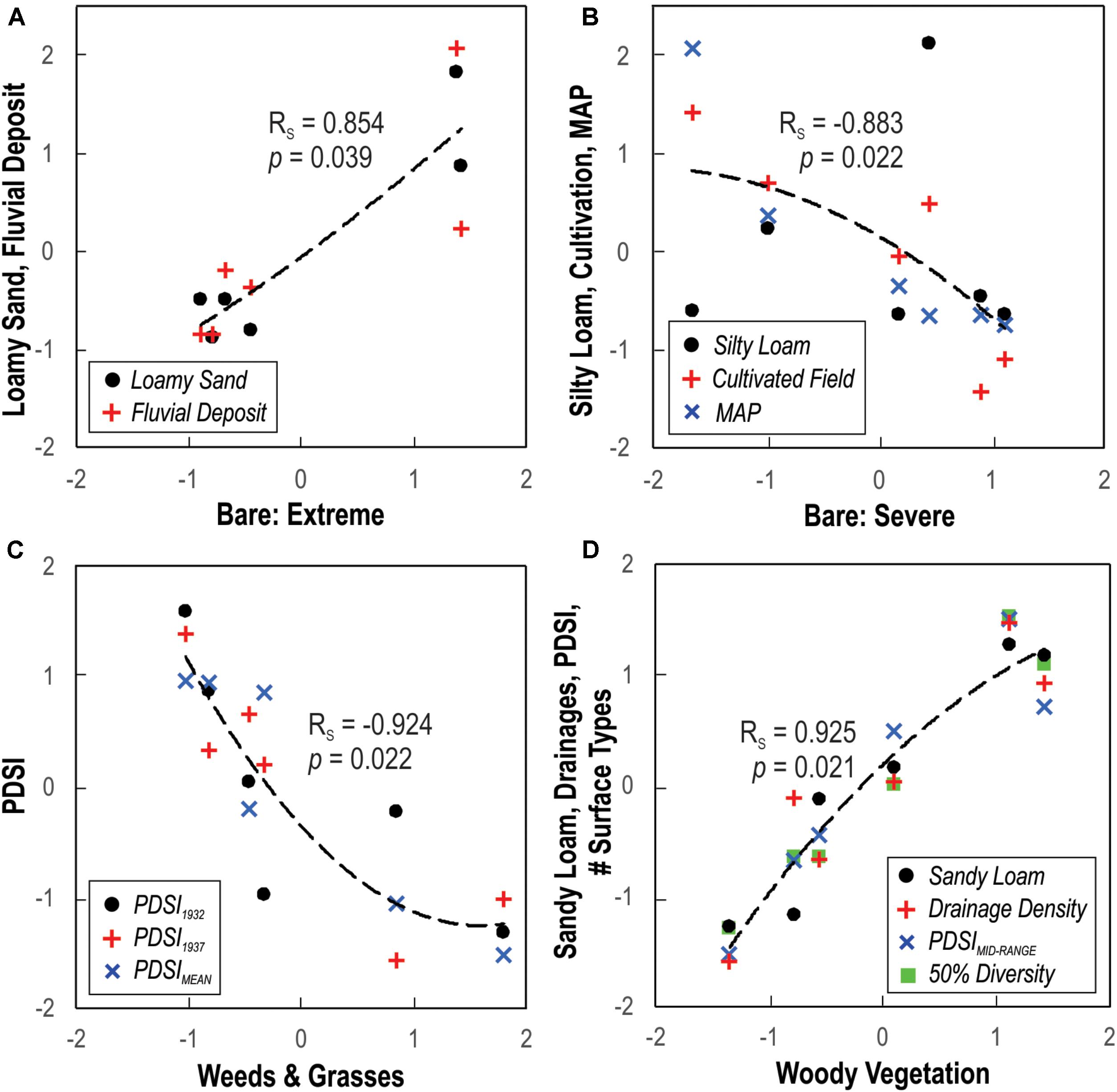
FIGURE 8. Scatter plots of selected variable pairs receiving a Spearman’s rank correlation coefficient (RS) equal to or over ± 0.8 and where p ≤ 0.05 exhibit monotonic relationships between land cover, sediment texture, land use, and/or climatic factors: (A) area of extremely bare surfaces increases with area of loamy sand soils and fluvial deposits; (B) extent of severely bare surfaces increases where areas of silty loam soils and mapped cultivated fields decrease, and where mean annual precipitation (MAP) is lower; (C) cover of patchy weeds and grasses increases in counties where the Palmer Drought Severity Index (PDSI) is lower in 1932, 1937, and in the overall mean from 1931 to 1940; and (D) the densest, woody vegetation increases in coverage with areas of sandy loam soils, greater density of fluvial drainages, a higher mid-range PDSI from 1931 to 1940, and the number of surface types explaining at least half of the total surface area (50% Diversity).
Principal component analysis reduces the 52 variables included to three PCs that explain >80% of the variance, and >90% of the variance is accounted for by including the fourth PC (Figures 9A,B). In component space, Ward County, ND plots in the lower quintile of the first three PCs, most closely associated with silty loam and silty clay loam soils, grassland, lacustrine basins, and change in maximum MAT. McPherson County, NE ranks in the lower quintile of PC1 and the upper quintile of PC3, with weed and grass cover and the average percentage of sand in county soils. Hamilton County, KS falls in the lower quintile of PC1 and the upper quintile of PC2, most closely associated with areas of mapped sand, clay loam soils, sandsheets, and the percentage of area uncultivated by 1935. Quay County, NM is in the upper quintile of PC2, generally correlated with areas of exposed bedrock, dunes, and moderately-to-extremely denuded surfaces. Tillman County, OK is in the upper quintile of PC1, most closely associated with: the total count of surface types classified, summer PDSI of 1934, 1935, and mid-range during the DBD, drainage density, and occurrence of sandy loam soils and woody vegetation. Lamar County, TX plots in the upper quintiles of PC1 and PC3, and in addition to the variables associated with Tillman County, is also correlated with 50% and 90% diversity thresholds in surface type, clay soils, percentage of land cultivated by 1935, and MAP.
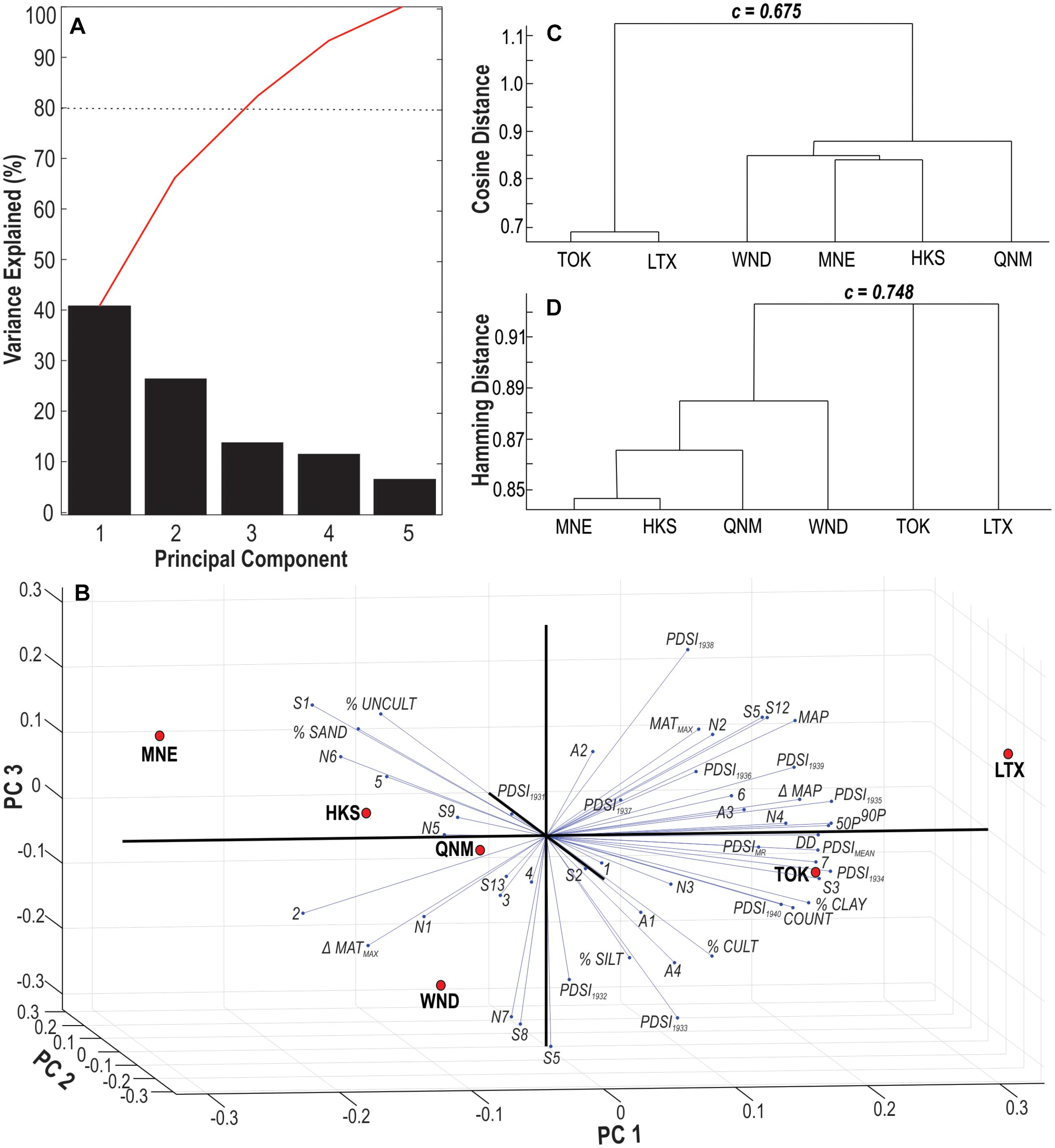
FIGURE 9. Multivariate statistical analyses of surface types by location in Ward County, ND (WND), McPherson County, NE (MNE), Hamilton County, KS (HKS), Quay County, NM (QNM), Tillman County, OK (TOK) and Lamar County, TX (LTX): (A) Scree plot of principal components, (B) Triplot of the first three principal components, (C) dendrogram of hierarchical clusters measured by cosine distance and (D) hamming distance, with cophenetic correlation coefficient, c.
As the PCA indicates four components explain >90% of the variance between sites, four hierarchical clusters elucidate the covariance in surficial response across sites. Cosine distance of site linkages provides a relatively reliable cluster tree, with a cophenetic correlation coefficient (c) of 0.676 (Figure 9C), though hamming distance determines a somewhat stronger correlation (c = 0.748, Figure 9D). The former measure demarcates four clusters as: (1) Tillman County, OK and Lamar County, TX, (2) Quay County, NM, (3) Ward County, ND, and (4) McPherson County, NE and Hamilton County, KS. For both distance measures, the largest break occurs between cluster 1 and clusters 2–4; however, cosine distance closely links Tillman and Lamar counties where hamming distance creates a discrete separation. Likewise, cosine distance calculates close linkages amongst clusters 2, 3, and 4 where hamming distance estimates more distinct, gradational steps between sites.
Discussion
Ecoregional Response to the Dust Bowl
The DBD is a vivid example for an annual record of drought on the USGP, though is modest in intensity and duration compared to droughts in the past 1,000 years (Cook et al., 2007, 2010; Woodhouse et al., 2010) and forecasted droughts for the 21st and 22nd centuries (Cook et al., 2015). Spatial analysis of countywide anomalies in maximum MAT, MAP, and PDSI from 1931 to 1940, concomitant with average soil texture, density of linear water features, and extent cultivated by 1935, illuminates the magnitude of DBD aridity in USGP counties and surficial coherence within ecoregions. The distribution of the highest ranked counties (8) reveals a cluster of impacted counties on the northern USGP in the Dakotas (Figure 5G). The greater clastic influx between 1930 and 1950 observed in lake cores from the Dakotas and Minnesota underscores this regional aridity (Dean, 1997; Shapley et al., 2005; Wigdahl et al., 2014). Dust storms, like that observed November 12, 1933, moved progressively over Bismarck, ND and Omaha, NE, with suspended particles eventually raining out across southern and eastern states (Hovde, 1934; Miller, 1934). A less continuous cluster of southern counties occurs within the classically defined DBD area of severe wind erosion, constrained by a maximum MAT range of 20 to 25°C, MAP of >500 mm, and the ∼250 km eastward shift of this isohyet compared to the previous 35-year period (Figure 2). Interestingly, the highest ranked counties within this region are also where private hospitals were at capacity and Red Cross emergency hospitals were set-up to deal with a conspicuous increase in “dust pneumonia” (Chicago Tribune, 1935).
The apparent exception to this ranking system are the counties comprising the Nebraska Sand Hills, which ranked 4 and 5 despite persistent drought conditions. This suggests grassland response observed in this area may not be correlatable to other counties with respect to the surficial criteria included in the site selection overlay. The high infiltration capacity of sandy soils in tandem with the high levels of regional groundwater tables contribute to the dominance of baseflow control on local response, and baseflow is generally resistant to interannual climate variability (Wang et al., 2009). On annual time-scales the Sand Hills generate higher rates of mean runoff and recharge, correlated with lower actual evapotranspiration, than in adjacent areas with siltier soils and relative to the amount of precipitation received (Gosselin et al., 2006; Harvey et al., 2007; Wang et al., 2009). The consistency of groundwater levels since AD 1700 appears to buffer the impact of the DBD in this region of Nebraska. However, multi-decadal droughts during the MCA (∼AD 800–1200) were sufficiently severe for a regional decline in the water table, with concomitant landscape denudation and increase of eolian transport and deposition (e.g., Harvey et al., 2007; Miao et al., 2007; Halfen and Johnson, 2013).
Influence of Surficial Properties and Climate on USGP Landscape Degradation
The spread of landscape degradation identified reflects ephemeral and cumulative effects of multiple controls that vary with antecedent landscape conditions and persistence of climatic anomalies (Turner, 1989; Schlesinger et al., 1990; Peters et al., 2007; He, 2014; Petrie et al., 2016). PCA indicates that site variance largely parallels location east or west of the 100th meridian, coupled with the severity of the precipitation deficit during the 1930s. The secondary component is related to the latitudinal temperature gradient and predominant land use and geomorphology, with a tertiary influence from soil texture and/or the annual PDSI during the DBD. Similar studies of USGP grasslands find that many ecosystem processes are primarily driven by precipitation and modified by temperature (Petrie et al., 2016; Nielsen, 2018; Seager et al., 2018). This analysis is also consistent with a linear relationship between drought intensity and ecosystem resistance observed in a global analysis of grassland response to ∼500 drought events (Ruppert et al., 2015).
Clustering analysis illustrates the differences in landscape stability across the arid-to-humid divide. Biotic controls tend to drive ecosystem stability east of the 100th meridian, with increased plant functional diversity and greater below-ground biomass of woody species (He, 2014; Lei et al., 2016). Both Tillman County, OK and Lamar County, TX, are characterized by mostly continuous dense or woody vegetation increasing with areas of greater soil clay content, near-river landforms, and reduced temperature anomalies, likely reflecting water availability. Tallgrass prairie is generally resistant to inter-annual precipitation variability and resilient to daily or weekly extremes (Jones et al., 2016), and more sensitive to monthly and seasonal precipitation distribution (Petrie et al., 2016). The distribution of the densest vegetation cover in this region is most strongly correlated with the summer PDSI of 1934 and 1935. This association would suggest ecosystem degradation in the eastern USGP was largely driven by plant response to the magnitude shift in seasonal conditions from 1934, recognized as the most severe drought year of the last millennium (Cook et al., 2014), to 1935, a wet period for the southeastern USGP (Figure 3E). Noteworthy in Lamar County, TX are the relict nebkha dunes revealed at the surface in areas cleared for cultivation. These features are similar to sites dated to 700–1,000 year BP on the Ozark Plateau and underscore the spatial extent and intensity of MCA droughts in the late Holocene (e.g., Seifert et al., 2009).
Abiotic controls appear to more strongly influence grassland degradation west of the 100th meridian and are associated with latitudinal temperature effects (Nielsen, 2018). The northern ecoregion of Ward County, ND experienced some of the most pronounced increases in maximum temperature during the DBD but is largely detached from other western sites in component space related to the overall lower MAT and dominance of siltier soils. Quay County, NM is likewise clustered individually but is near in component space to Tillman County, OK, as both are southern ecoregions with milder DBD conditions, and shows a greater diversity of surface types than other western counties. Nonetheless, this area of eastern New Mexico is statistically linked to Hamilton County, KS and McPherson County, NE, and correlated with the distribution of increasingly sandy soils and large patches of eolian landforms indicative of soil erosion. These latter two counties are both central ecoregions with a similar distribution of land use, high soil sand content, and exhibit less surficial diversity than eastern sites as sandsheets and dunes cascade across the landscape. McPherson County is influenced by groundwater levels at the margins of the Sand Hills and classified as mostly vegetated sandsheet and interdunal grassland with little change to extent of cultivation. Whereas Hamilton County shows ∼50% vegetation loss of shortgrass prairie, associated with active eolian landforms and a sharp increase in apparently fallow fields.
Broadly, the distribution of denuded surfaces during the DBD exhibits stronger non-parametric correlations with surficial properties than climatic factors. Land use interacts with degradation regardless of setting but is more significant to explain site variance in eastern counties, whereas uncultivated landforms dominate the drier, western areas. Sand-dominated soil textures on landscapes with maximum relief are correlated with more frequent denudation for western counties. The areal extent of blow-outs, parabolic dunes, sinuous ridges, and sandsheets positively covary, and this heterogenous landform assemblage correlates to intensity and persistence of 1930s aridity (Hugenholtz and Wolfe, 2005, 2006). Particle sources for the DBD have been attributed solely to areas of agricultural disturbance in the south-central Great Plains (cf. Bennett and Fowler, 1936; Johnson, 1947; Worster, 1982; Hansen and Libecap, 2004; Schubert et al., 2004; Cook et al., 2008, 2009; Lee and Gill, 2015). This analysis identifies large uncultivated areas that were equally or more a source of dust during the DBD than plowed agricultural fields. On the Northern Great Plains (North Dakota), one significant source of dust is with the drop of lake level and the exposure of lake sediments and adjacent eolian deposits. In the classic DBD area, the many stabilized, high-relief sand-rich dune systems adjacent to major rivers were partially to wholly denuded and were significant sources of dust.
Implications for Future USGP Grassland Response to Drought
A similar shift in the arid-to-humid transition as observed during the 1930s is projected for the future, which can strongly influence settlement sustainability and agricultural development (Nielsen, 2018; Seager et al., 2018). The overuse of groundwater coupled with rising costs of irrigation could cause groundwater tables to lower and increase susceptibility of previously stable systems (Parton et al., 2007). Future warming may reduce vegetation cover and soil moisture over large areas of USGP grasslands, exacerbating soil erosion, degradation feedbacks, and decline of terrestrial carbon sinks (Schlesinger et al., 1990; Lei et al., 2016; Hu et al., 2018). Regional hydroclimatic variability and carbon sequestration is therefore dependent on how land surface changes modulate climatic conditions (Cook et al., 2013; Petrie et al., 2016; Hu et al., 2018). Given the potential speed and irreversibility of such changes (Breshears and Barnes, 1999; Collins et al., 2014; Moran et al., 2014; Svejcar et al., 2015), characterizing USGP grassland response during severe drought is significant to constrain the large variability in landscape degradation (Petrie et al., 2016), and to better guide adaptable land and carbon management (Basara et al., 2013; Ruppert et al., 2015; Lei et al., 2016; Petrie et al., 2016; Byrne et al., 2017).
Conclusion
The wealth of images and associated documentation for the 1930s Dust Bowl enables quantitative evaluation of land surface processes and inferred vegetation changes on a regional- to sub-meter scale. The extent of landscape degradation during this historic drought was assessed across a latitudinal temperature and longitudinal precipitation gradient for the USGP from historical aerial negatives acquired from six representative counties to better understand biotic and abiotic processes during the nearly decade-long drought. During the DBD, the 500 mm isohyet shifted several hundred kilometers to the east. The surficial response on the USGP during the DBD is found to most strongly correlate with this redistributed arid–humid divide, the magnitude of precipitation and temperature anomalies, and soil texture. Similar surficial response to the DBD was observed from sites within the same ecoregion, highlighting the role of dominant species and functional diversity of plants (Lei et al., 2016) and a nearly linear relationship with intensity of aridity (Schlesinger et al., 1990; Tongway and Ludwig, 1994; Ravi et al., 2010; Bestelmeyer et al., 2011; Ruppert et al., 2015).
The dominant sources of degradation found for study sites east of the 100th meridian were cultivated fields and fluvial deposits, associated with woody vegetation response to water availability in uncultivated areas. For sites to the west, denuded surfaces are predominantly eolian sandsheets and dunes, correlated with intensity of drought conditions and reduced plant diversity. Discrete spatial signatures of the drought are observed not only within the classically recognized southern Dust Bowl area, but also in the northern and central plains, suggesting a much larger regional response to the drought than previously recognized. The source of the namesake dust storms of the DBD has hitherto been attributed solely to areas of agricultural disturbance in the south-central Great Plains (cf. Bennett and Fowler, 1936; Johnson, 1947; Worster, 1982; Hansen and Libecap, 2004; Schubert et al., 2004; Cook et al., 2008, 2009; Lee and Gill, 2015). This analysis demonstrates the potential of locally denuded, uncultivated, sand-rich areas across the USGP as equivalent or greater sources for particle emission during intense drought than plowed agricultural fields. The USGP is forecast to become more vulnerable to drought stress in the 21st century, with increasing demands on water resources and concomitant increase in dominance of abiotic drivers, which could precipitate a landscape response similar to the DBD (Ravi et al., 2010; Woodhouse et al., 2010; Basara et al., 2013; Cook et al., 2015).
Author Contributions
KB and SF conceived of the project and both performed archival research of historical documentation. KB spearheaded image processing and analysis and manuscript preparation. SF provided guidance throughout the study and assisted in manuscript preparation.
Funding
This research was supported by the National Geographic Society (#9990-16), the National Science Foundation Award GSS-1660230, and the Glasscock Endowed Fund for Excellence in Environmental Science (032MBCU31).
Conflict of Interest Statement
The authors declare that the research was conducted in the absence of any commercial or financial relationships that could be construed as a potential conflict of interest.
Acknowledgments
We are grateful to National Archives staff for research assistance and material access and to Dirk Burgdorf of AAA Research for aerial photograph reproduction.
References
Albertson, F. W., and Weaver, J. E. (1944). Nature and degree of recovery of grassland from the great drought of 1933 to 1940. Ecol. Monogr. 14, 393–479. doi: 10.2307/1948617
Anderson, J. J., and Cobb, N. S. (2004). Tree cover discrimination in panchromatic aerial imagery of pinyon-juniper woodlands. Photogrammet. Eng. Remote Sens. 70, 1063–1068. doi: 10.14358/PERS.70.9.1063
Baddock, M. C., Ginoux, P., Bullard, J. E., and Gill, T. E. (2016). Do MODIS-defined dust sources have a geomorphological signature?: Geomorphology and dust emission. Geophys. Res. Lett. 43, 2606–2613. doi: 10.1002/2015GL067327
Bakker, M., and Lane, S. N. (2017). Archival photogrammetric analysis of river–floodplain systems using Structure from Motion (SfM) methods. Earth Surface Process. Landforms 42, 1274–1286. doi: 10.1002/esp.4085
Ball, G. H., and Hall, D. J. (1967). A clustering technique for summarizing multivariate data. Behav. Sci. 12, 153–155. doi: 10.1002/bs.3830120210
Basara, J. B., Maybourn, J. N., Peirano, C. M., Tate, J. E., Brown, P. J., Hoey, J. D., et al. (2013). Drought and associated impacts in the great plains of the united states—A review. Int. J. Geosci. 4, 72–81. doi: 10.4236/ijg.2013.46A2009
Bastin, G. N., Ludwig, J. A., Eager, R. W., Chewings, V. H., and Liedloff, A. C. (2002). Indicators of landscape function: comparing patchiness metrics using remotely–sensed data from rangelands. Ecol. Indic. 1, 247–260. doi: 10.1016/S1470-160X(02)00009-2
Bel, G., and Ashkenazy, Y. (2014). The effects of psammophilous plants on sand dune dynamics. J. Geophys. Res. Earth Surface 119, 1636–1650. doi: 10.1002/2014JF003170
Belnap, J., Munson, S. M., and Field, J. P. (2011). Aeolian and fluvial processes in dryland regions: the need for integrated studies. Ecohydrology 4, 615–622. doi: 10.1002/eco.258
Ben-Dor, E. (2002). Quantitative remote sensing of soil properties. Adv. Agron. 75, 173–244. doi: 10.1016/S0065-2113(02)75005-0
Bennett, H. H., and Fowler, F. H. (1936). Report of the Great Plains Drought Area Committee. Washington, DC: Government Printing Office.
Bestelmeyer, B. T., Ward, J. P., and Havstad, K. M. (2011). Analysis of abrupt transitions in ecological systems. Ecosphere 2:129.
Blaschke, T., Hay, G. J., Kelly, M., Lang, S., Hofmann, P., Addink, E., et al. (2014). Geographic object–based image analysis–towards a new paradigm. ISPRS J. Photogramm. Remote Sens. 87, 180–191. doi: 10.1016/j.isprsjprs.2013.09.014
Bolles, K., Forman, S. L., and Sweeney, M. (2017). Eolian processes and heterogeneous dust emissivity during the 1930s dust bowl drought and implications for projected 21st–century megadroughts. Holocene 27, 1578–1588. doi: 10.1177/0959683617702235
Borradaile, G. (ed.). (2003). “Correlation and comparison of variables,” in Statistics of Earth Science Data (Berlin: Springer), 157–185. doi: 10.1007/978-3-662-05223-5_7
Breshears, D. D., and Barnes, F. J. (1999). Interrelationships between plant functional types and soil moisture heterogeneity for semiarid landscapes within the grassland/forest continuum: a unified conceptual model. Landsc. Ecol. 14, 465–478. doi: 10.1023/A:1008040327508
Browning, D. M., Archer, S. R., and Byrne, A. T. (2009). Field validation of 1930s aerial photography: What are we missing? J. Arid Environ. 73, 844–853. doi: 10.1016/j.jaridenv.2009.04.003
Byrne, K. M., Adler, P. B., and Lauenroth, W. K. (2017). Contrasting effects of precipitation manipulations in two great plains plant communities. J. Veg. Sci. 28, 238–249. doi: 10.1111/jvs.12486
Carmel, Y., and Kadmon, R. (1998). Computerized classification of Mediterranean vegetation using panchromatic aerial photographs. J. Veg. Sci. 9, 445–454. doi: 10.2307/3237108
Chicago Tribune (1935). Ninth victim of dust pneumonia dies in Kansas. Available at: https://chicagotribune.newspapers.com/
Collins, S. L., Belnap, J., Grimm, N. B., Rudgers, J. A., Dahm, C. N., D’Odorico, P., et al. (2014). A multiscale, hierarchical model of pulse dynamics in arid–land ecosystems. Ann. Rev. Ecol. Evol. Syst. 45, 397–419. doi: 10.1146/annurev-ecolsys-120213-091650
Collins, S. L., Knapp, A. K., Briggs, J. M., Blair, J. M., and Steinauer, E. M. (1998). Modulation of diversity by grazing and mowing in native tallgrass prairie. Science 280, 745–747. doi: 10.1126/science.280.5364.745
Cook, B., Ault, T. R., and Smerdon, J. E. (2015). Unprecedented 21st century drought risk in the american southwest and central plains. Sci. Adv. 1:e1400082.
Cook, B., Cook, E. R., Anchukaitis, K. J., Seager, R., and Miller, R. L. (2011a). Forced and unforced variability of twentieth century North American droughts and pluvials. Clim. Dyn. 37, 1097–1110.
Cook, B., Seager, R., and Miller, R. L. (2011b). The impact of devegetated dune fields on North American climate during the late medieval climate anomaly: dunes and medieval climate. Geophys. Res. Lett. 38:L14074.
Cook, B., Miller, R. L., and Seager, R. (2008). Dust and sea surface temperature forcing of the 1930s “Dust Bowl” drought. Geophys. Res. Lett. 35:L08710. doi: 10.1029/2008GL033486
Cook, B., Miller, R. L., and Seager, R. (2009). Amplification of the North American “dust bowl” drought through human–induced land degradation. Proc. Natl. Acad. Sci. U.S.A. 106, 4997–5001. doi: 10.1073/pnas.0810200106
Cook, B., Seager, R., Miller, R. L., and Mason, J. A. (2013). Intensification of north american megadroughts through surface and dust aerosol forcing∗. J. Clim. 26, 4414–4430. doi: 10.1175/JCLI-D-12-00022.1
Cook, B., Seager, R., and Smerdon, J. E. (2014). The worst North American drought year of the last millennium: 1934. Geophys. Res. Lett. 41, 7298–7305. doi: 10.1002/2014GL061661
Cook, E. R., Seager, R., Cane, M. A., and Stahle, D. W. (2007). North american drought: reconstructions, causes, and consequences. Earth Sci. Rev. 81, 93–134. doi: 10.1016/j.earscirev.2006.12.002
Cook, E. R., Seager, R., Heim, R. R., Vose, R. S., Herweijer, C., and Woodhouse, C. (2010). Megadroughts in North America: placing IPCC projections of hydroclimatic change in a long–term palaeoclimate context. J. Quat. Sci. 25, 48–61. doi: 10.1002/jqs.1303
Cordova, C. E., Porter, J., Lepper, K., Kalchgruber, R., and Scott, G. (2005). Preliminary assessment of sand dune stability along a bioclimatic gradient, North Central and Northwestern Oklahoma. Great Plains Res. J. Nat. Soc. Sci. Paper 783, 227–249.
Cunfer, G. (2005). On the Great Plains: Agriculture and Environment, 1st Edn. College Station, TX: Texas A&M University Press.
Dean, W. E. (1997). Rates, timing, and cyclicity of holocene eolian activity in north–central United States: evidence from varved lake sediments. Geology 25:331.
Derickson, D., Kocurek, G., Ewing, R. C., and Bristow, C. (2008). Origin of a complex and spatially diverse dune–field pattern, Algodones, southeastern California. Geomorphology 99, 186–204. doi: 10.1016/j.geomorph.2007.10.016
Derner, J. D., Boutton, T. W., and Briske, D. D. (2006). Grazing and ecosystem carbon storage in the North American great plains. Plant Soil 280, 77–90. doi: 10.1007/s11104-005-2554-3
Donat, M. G., King, A. D., Overpeck, J. T., Alexander, L. V., Duure, I., and Karoly, D. J. (2016). Extraordinary heat during the 1930s US Dust Bowl and associated large–scale conditions. Clim. Dynam. 46, 413–426. doi: 10.1007/s00382-015-2590-5
Doneus, M., Wieser, M., Verhoeven, G., Karel, W., Fera, M., and Pfeifer, N. (2016). Automated archiving of archaeological aerial images. Remote Sens. 8:209.
Escadafal, R., and Huete, A. R. (1992). “Soil optical properties and environmental applications of remote sensing,” in Proceedings of the Technical Commission VII: Interpreation of Photoaphic and Remote Sensing Data, Washington, DC, 709–715.
Evans, S. E., Byrne, K. M., Lauenroth, W. K., and Burke, I. C. (2011). Defining the limit to resistance in a drought–tolerant grassland: long–term severe drought significantly reduces the dominant species and increases ruderals. J. Ecol. 99, 1500–1507.
Ewing, R. C., and Kocurek, G. (2010). Aeolian dune–field pattern boundary conditions. Geomorphology 114, 175–187. doi: 10.1016/j.geomorph.2009.06.015
Ewing, R. C., Kocurek, G., and Lake, L. W. (2006). Pattern analysis of dune–field parameters. Earth Surface Process. Landforms 31, 1176–1191. doi: 10.1002/esp.1312
Forman, S. L., Marín, L., Gomez, J., and Pierson, J. (2008). Late quaternary eolian sand depositional record for southwestern kansas: landscape sensitivity to droughts. Palaeogeogr. Palaeoclimatol. Palaeoecol. 265, 107–120. doi: 10.1016/j.palaeo.2008.04.028
Forman, S. L., Marín, L., Pierson, J., Gomez, J., Miller, G. H., and Webb, R. S. (2005). Aeolian sand depositional records from western Nebraska: landscape response to droughts in the past 1500 years. Holocene 15, 973–981. doi: 10.1191/0959683605hl871ra
Gennaretti, F., Ripa, M. N., Gobattoni, F., Boccia, L., and Pelorosso, R. (2011). A methodology proposal for land cover change analysis using historical aerial photos. J. Geogr. Reg. Plann. 4, 542–556.
Giordano, S., Le Bris, A., and Mallet, C. (2017). “Fully automatic analysis of archival aerial images current status and challenges,” in Proceedings of the Urban Remote Sensing Event (JURSE), 2017 (Piscataway, NJ: IEEE), 1–4.
Gomez, C. (2012). Historical 3D Topographic Reconstruction of the Iwaki Volcano Using Structure from Motion From Uncalibrated Aerial Photographs. Available at: https://hal.archives-ouvertes.fr/hal-00765723
Gonçalves, J. A. (2016). Automatic orientation and mosaicking of archived aerial photography using structure from motion. ISPRS – Int. Arch. Photogramm. Remote Sens. Spat. Inform. Sci. XL–3/W4, 123–126. doi: 10.5194/isprsarchives-XL-3-W4-123-2016
Gosselin, D. C., Sridhar, V., Harvey, F. E., and Goeke, J. W. (2006). Hydrological effects and groundwater fluctuations in interdunal environments in the Nebraska Sand Hills. Great Plains Res. 16:12.
Gutmann, M. P. (2005). Great Plains Population and Environment Data: Agricultural Data, 1870-1997 [United States]. Ann Arbor, MI: Inter-university Consortium for Political and Social Research [distributor]. doi: 10.3886/ICPSR04254.v1 (accessed May 2017).
Halfen, A. F., and Johnson, W. C. (2013). A review of Great plains dune field chronologies. Aeolian Res. 10, 135–160. doi: 10.1016/j.aeolia.2013.03.001
Hansen, Z. K., and Libecap, G. D. (2004). Small farms, externalities, and the Dust Bowl of the 1930s. J. Polit. Econ. 112, 665–694. doi: 10.1086/383102
Haralick, R. M., Shanmugam, K., and Dinstein, I. H. (1973). Textural features for image classification. IEEE Trans. Syst. Man Cybernet. 3, 610–621. doi: 10.1109/TSMC.1973.4309314
Harvey, F. E., Swinehart, J. B., and Kurtz, T. M. (2007). Ground water sustenance of nebraska’s unique sand hills peatland fen ecosystems. Ground Water 45, 218–234. doi: 10.1111/j.1745-6584.2006.00278.x
He, Y. (2014). The effect of precipitation on vegetation cover over three landscape units in a protected semi–arid grassland: temporal dynamics and suitable climatic index. J. Arid Environ. 109, 74–82. doi: 10.1016/j.jaridenv.2014.05.022
Heipke, C. (1997). Automation of interior, relative, and absolute orientation. ISPRS J. Photogramm. Remote Sens. 52, 1–19. doi: 10.1016/S0924-2716(96)00029-9
Hovde, M. R. (1934). The great dust storm of November 12, 1933. Mon. Weather Rev. 62, 12–13. doi: 10.1175/1520-0493 (1934)62<12:TGDON>2.0.CO;2
Hu, Q., Torres-Alavez, J. A., and Van Den Broeke, M. S. (2018). Land–cover change and the “Dust bowl” drought in the US Great plains. J. Clim. 31, 4657–4667. doi: 10.1175/JCLI-D-17-0515.1
Hugenholtz, C. H., and Wolfe, S. A. (2005). Biogeomorphic model of dunefield activation and stabilization on the northern Great Plains. Geomorphology 70, 53–70. doi: 10.1016/j.geomorph.2005.03.011
Hugenholtz, C. H., and Wolfe, S. A. (2006). Morphodynamics and climate controls of two aeolian blowouts on the northern Great Plains, Canada. Earth Surface Process. Landforms 31, 1540–1557. doi: 10.1002/esp.1367
Hunt, G. R., and Salisbury, J. W. (1970). Visible and near infrared spectra of minerals and rocks: I: silicate minerals. Modern Geol. 1, 283–300.
Jones, S. K., Collins, S. L., Blair, J. M., Smith, M. D., and Knapp, A. K. (2016). Altered rainfall patterns increase forb abundance and richness in native tallgrass prairie. Sci. Rep. 6:20120.
Jurena, P. N., and Archer, S. (2003). Woody plant establishment and spatial heterogeneity in grasslands. Ecology 84, 907–919. doi: 10.1890/0012-9658 (2003)084[0907:WPEASH]2.0.CO;2
Kadmon, R., refauthand Harari-Kremer, R. (1999). Studying long–term vegetation dynamics using digital processing of historical aerial photographs. Remote Sens. Environ. 68, 164–176. doi: 10.1016/S0034-4257(98)00109-6
Koerner, S. E., and Collins, S. L. (2014). Interactive effects of grazing, drought, and fire on grassland plant communities in North America and South Africa. Ecology 95, 98–109. doi: 10.1890/13-0526.1
Konings, A. G., Williams, A. P., and Gentine, P. (2017). Sensitivity of grassland productivity to aridity controlled by stomatal and xylem regulation. Nat. Geosci. 10, 284–288. doi: 10.1038/ngeo2903
Laird, K. R., Fritz, S. C., and Cumming, B. F. (1998). A diatom–based reconstruction of drought intensity duration and frequency from Moon Lake North Dakota: a sub–decadal record of the last 2300 years. J. Paleolimnol. 19, 161–179. doi: 10.1023/A:1007929006001
Laliberte, A. S., Rango, A., Havstad, K. M., Paris, J. F., Beck, R. F., McNeely, R., et al. (2004). Object–oriented image analysis for mapping shrub encroachment from 1937 to 2003 in southern New Mexico. Remote Sens. Environ. 93, 198–210. doi: 10.1016/j.rse.2004.07.011
Lee, J. A., and Gill, T. E. (2015). Multiple causes of wind erosion in the Dust Bowl. Aeol. Res. 19, 15–36. doi: 10.1016/j.aeolia.2015.09.002
Leedy, D. L. (1948). Aerial photographs, their interpretation and suggested uses in wildlife management. J. Wildlife Manage. 12, 191. doi: 10.2307/3796415
Lei, T., Pang, Z., Wang, X., Li, L., Fu, J., Kan, G., et al. (2016). Drought and carbon cycling of grassland ecosystems under global change: a review. Water 8:460.
Lepper, K., and Scott, G. F. (2005). Late holocene aeolian activity in the cimarron river valley of west–central Oklahoma. Geomorphology 70, 42–52. doi: 10.1016/j.geomorph.2005.03.010
Li, H., and Reynolds, J. F. (1995). On definition and quantification of heterogeneity. Oikos 73, 280–284. doi: 10.2307/3545921
Lishawa, S. C., Treering, D. J., Vail, L. M., McKenna, O., Grimm, E. C., and Tuchman, N. C. (2013). Reconstructing plant invasions using historical aerial imagery and pollen core analysis: typha in the laurentian great lakes. Diversity Distribut. 19, 14–28. doi: 10.1111/j.1472-4642.2012.00929.x
Liu, B., and Coulthard, T. J. (2015). Mapping the interactions between rivers and sand dunes: Implications for fluvial and aeolian geomorphology. Geomorphology 231, 246–257. doi: 10.1016/j.geomorph.2014.12.011
Liu, B., and Coulthard, T. J. (2017). Modelling the interaction of aeolian and fluvial processes with a combined cellular model of sand dunes and river systems. Comput. Geosci. 106, 1–9. doi: 10.1016/j.cageo.2017.05.003
Liu, J. G., and Mason, P. J. (2016). Image Processing and GIS for Remote Sensing: Techniques and Applications. Hoboken, NJ: John Wiley & Sons. doi: 10.1002/9781118724194
Maestre, F. T., Cortina, J., Bautista, S., Bellot, J., and Vallejo, R. (2003). Small–scale environmental heterogeneity and spatiotemporal dynamics of seedling establishment in a semiarid degraded ecosystem. Ecosystems 6, 630–643. doi: 10.1007/s10021-002-0222-5
Mason, J. A., Swinehart, J. B., Goble, R. J., and Loope, D. B. (2004). Late–Holocene dune activity linked to hydrological drought, Nebraska Sand Hills, USA. Holocene 14, 209–217. doi: 10.1191/0959683604hl677rp
Mather, P. M., and Koch, M. (2011). Computer Processing of Remotely–Sensed Images: An Introduction, 4th Edn. Chichester: Wiley–Blackwell. doi: 10.1002/9780470666517
Mertes, J. R., Gulley, J. D., Benn, D. I., Thompson, S. S., Nicholson, L. I. (2017). Using structure–from–motion to create glacier DEMs and orthoimagery from historical terrestrial and oblique aerial imagery: SfM on differing historical glacier imagery sets. Earth Surface Process. Landforms 42, 2350–2364. doi: 10.1002/esp.4188
Meyers, T. P. (2001). A comparison of summertime water and CO2 fluxes over rangeland for well watered and drought conditions. Agric. For. Meteorol. 106, 205–214. doi: 10.1016/S0168-1923(00)00213-6
Miao, X., Mason, J. A., Swinehart, J. B., Loope, D. B., Hanson, P. R., Goble, R. J., et al. (2007). A 10,000 year record of dune activity, dust storms, and severe drought in the central Great Plains. Geology 35, 119–122. doi: 10.1130/G23133A.1
Miller, E. R. (1934). The dustfall of November 12–13, 1933. Mon. Weather Rev. 62, 14–15. doi: 10.1175/1520-0493 (1934)62<14:TDON>2.0.CO;2
Mölg, N., and Bolch, T. (2017). Structure–from–motion using historical aerial images to analyse changes in glacier surface elevation. Remote Sens. 9:1021. doi: 10.3390/rs9101021
Moran, M. S., Ponce-campos, G. E., Huete, A. R., and McClaran, M. P. (2014). Functional response of U.S. grasslands to the early 21st–century drought. Ecology 95, 2121–2133. doi: 10.1890/13-1687.1
Morgan, J. L., and Gergel, S. E. (2010). Quantifying historic landscape heterogeneity from aerial photographs using object–based analysis. Landsc. Ecol. 25, 985–998. doi: 10.1007/s10980-010-9474-1
Morgan, J. L., and Gergel, S. E. (2013). Automated analysis of aerial photographs and potential for historic forest mapping. Can. J. For. Res. 43, 699–710. doi: 10.1139/cjfr-2012-0492
Morgan, J. L., Gergel, S. E., and Coops, N. C. (2010). Aerial photography: a rapidly evolving tool for ecological management. BioScience 60, 47–59. doi: 10.1525/bio.2010.60.1.9
Murray, D. B., White, J. D., and Swint, P. (2013). Woody vegetation persistence and disturbance in central texas grasslands inferred from multidecadal historical aerial photographs. Rang. Ecol. Manage. 66, 297–304. doi: 10.2111/REM-D-11-00180.1
Nagarajan, S., and Schenk, T. (2016). Feature–based registration of historical aerial images by area minimization. ISPRS J. Photogramm. Remote Sens. 116, 15–23. doi: 10.1016/j.isprsjprs.2016.02.012
National Archives and Record Administration[NARA] (2017) “Aerial Photographs” in Cartographic and Architectural Records General Information Leaflet, Number 26. June 26. Available at: https://www.archives.gov/publications/general-info-leaflets/26–cartographic.html#aerial1
Nebiker, S., Lack, N., and Deuber, M. (2014). Building change detection from historical aerial photographs using dense image matching and object–based image analysis. Remote Sens. 6, 8310–8336. doi: 10.3390/rs6098310
Nielsen, D. C. (2018). Influence of latitude on the US great plains east–west precipitation gradient. Agric. Environ. Lett. 3, 1–5.
O’Brien, M. J., Beets, J. L., Warren, R. E., Hotrabhavananda, T., Barney, T. W., and Voigt, E. E. (1982). Digital enhancement and grey-level slicing of aerial photographs: techniques for archaeological analysis of intrasite variability. World Archaeol. 14, 173–190. doi: 10.1080/00438243.1982.9979858
Okeke, F., and Karnieli, A. (2006). Methods for fuzzy classification and accuracy assessment of historical aerial photographs for vegetation change analyses, part I: algorithm development. Int. J. Remote Sens. 27, 153–176. doi: 10.1080/01431160500166540
Pacina, J., and Popelka, J. (2017). Accuracy of digital surface models derived from archival aerial photographs. Case study for the czech republic. Geoinformatics FCE CTU 16:53. doi: 10.14311/gi.16.1.3
Parajuli, S. P., and Zender, C. S. (2017). Connecting geomorphology to dust emission through high–resolution mapping of global land cover and sediment supply. Aeolian Res. 27, 47–65. doi: 10.1016/j.aeolia.2017.06.002
Parajuli, S. P., Yang, Z. L., and Kocurek, G. (2014). Mapping erodibility in dust source regions based on geomorphology, meteorology, and remote sensing: Land cover and erodibility mapping. J. Geophys. Res. Earth Surface 119, 1977–1994. doi: 10.1002/2014JF003095
Parton, W. J., Gutmann, M. P., and Ojima, D. (2007). Long-term trends in population, farm income, and crop production in the great plains. BioScience 57, 737–747. doi: 10.1641/B570906
Peters, D. P. C., Osvaldo, E. S., Allen, C. D., Covich, A., and Brunson, M. (2007). Cascading events in linked ecological and socioeconomic systems. Front. Ecol. Environ. 5, 221–224. doi: 10.1890/1540-9295 (2007)5[221:CEILEA]2.0.CO;2
Petrie, M. D., Brunsell, N. A., Vargas, R., Collins, S. L., Glanagan, L. B., Hanan, N. P., et al. (2016). The sensitivity of carbon exchanges in Great Plains grasslands to precipitation variability. J. Geophys. Res. Biogeosci. 121, 280–294. doi: 10.1002/2015JG003205
Pickett, S. T., and Cadenasso, M. (1995). Landscpae ecology: spatial heterogeneity in ecological systems. Science 269, 331–334. doi: 10.1126/science.269.5222.331
PRISM Climate Group (2017). Historical Past Time Series Datasets. Oregon State University, Corvallis, OR. Available at: http://prism.oregonstate.edu (accessed October 2017).
Rango, A., Havstad, K., and Estell, R. (2011). The utilization of historical data and geospatial technology advances at the jornada experimental range to support western america ranching culture. Remote Sens. 3, 2089–2109. doi: 10.3390/rs3092089
Rango, A., Laliberte, A. S., and Winters, C. (2008). Role of aerial photos in compiling a long-term remote sensing data set. J. Appl. Remote Sens. 2:023541. doi: 10.1117/1.3009225
Ravi, S., Breshears, D. D., Huxman, T. E., and D’Odorico, P. (2010). Land degradation in drylands: interactions among hydrologic-aeolian erosion and vegetation dynamics. Geomorphology 116, 236–245. doi: 10.1016/j.geomorph.2009.11.023
Redecker, A. P. (2008). Historical aerial photographs and digital photogrammetry for impact analyses on derelict land sites in human settlement areas. Int. Arch. Photogramm. Remote Sens. Spat. Inf. Sci. 37, 5–10.
Redweik, P., Roque, D., Marques, A., Matildes, R., and Marques, F. (2009). Recovering Portugal aerial images repository. Int. Arch. Photogramm. Remote Sens. 38, 1–4.
Ruppert, J. C., Harmoney, K., Henkin, Z., Snyman, H. A., Sternberg, M., Willms, W., et al. (2015). Quantifying drylands’ drought resistance and recovery: the importance of drought intensity, dominant life history and grazing regime. Global Change Biol. 21, 1258–1270. doi: 10.1111/gcb.12777
Sala, O. E., Parton, W. J., Joyce, L. A., and Lauenroth, W. K. (1988). Primary production of the central grassland region of the United States. Ecology 69, 40–45. doi: 10.2307/1943158
Samson, F. B., Knopf, F. L., and Ostlie, W. R. (2004). Great plains ecosystems: past, present, and future. Wildlife Soc. Bull. 32, 6–15. doi: 10.2193/0091-7648 (2004)32[6:GPEPPA]2.0.CO;2
Schlesinger, W. H., Reynolds, J. F., Cunningham, G. L., Huenneke, L. F., Jarrell, W. M., Virginia, R. A., et al. (1990). Biological feedbacks in global desertification. Science 247, 1043–1048. doi: 10.1126/science.247.4946.1043
Schook, D. M., Rathburn, S. L., Friedman, J. M., and Wolf, J. M. (2017). A 184–year record of river meander migration from tree rings, aerial imagery, and cross sections. Geomorphology 293, 227–239. doi: 10.1016/j.geomorph.2017.06.001
Schowengerdt, R. A. (2012). Techniques for Image Processing and Classifications in Remote Sensing. Cambridge: Academic Press.
Schubert, S. D., Suarez, M. J., Pegion, P. J., Koster, R. D., and Bacmeister, J. T. (2004). On the cause of the 1930s Dust Bowl. Science 303, 1855–1859. doi: 10.1126/science.1095048
Seager, R., Lis, N., Feldman, J., Ting, M., Williams, A. P., Nakamura, J., et al. (2018). Whither the 100th Meridian? The once and future physical and human geography of America’s Arid–Humid divide. Part I: the story so far. Earth Interact. 22, 1–22. doi: 10.1175/EI-D-17-0011.1
Seifert, C. L., Cox, R. T., Forman, S. L., Foti, T. L., Wasklewicz, T. A., and McColgan, A. T. (2009). Relict nebkhas (pimple mounds) record prolonged late Holocene drought in the forested region of south–central United States. Quat. Res. 71, 329–339. doi: 10.1016/j.yqres.2009.01.006
Sevara, C., Verhoeven, G., Doneus, M., and Draganits, E. (2018). Surfaces from the visual past: recovering high–resolution terrain data from historic aerial imagery for multitemporal landscape analysis. J. Archaeol. Method Theory 25, 611–642. doi: 10.1007/s10816-017-9348-9
Shapley, M. D., Johnson, W. C., Engstrom, D. R., and Osterkamp, W. R. (2005). Late-holocene flooding and drought in the Northern Great Plains, USA, reconstructed from tree rings, lake sediments and ancient shorelines. Holocene 15, 29–41. doi: 10.1191/0959683605hl781rp
Sims, P. L., and Bradford, J. A. (2001). Carbon dioxide fluxes in a southern plains prairie. Agric. For. Meteorol. 109, 117–134. doi: 10.1016/S0168-1923(01)00264-7
Skaggs, R., Edwards, Z., Bestelmeyer, B. T., Wright, J. B., Williamson, J., and Smith, P. (2011). Vegetation maps at the passage of the Taylor Grazing Act (1934): a baseline to evaluate rangeland change after a regime shift. Rangelands 33, 13–19. doi: 10.2111/RANGELANDS-D-10-00031.1
Skirvin, S. M., Kepner, W. G., March, S. E., Drake, S. E., Maingi, J. K., Edmonds, C. M., et al. (2004). Assessing the accuracy of satellite–derived land–cover classification using historical aerial photography, digital orthophoto quadrangles, and airborne video data. Remote Sens. GIS Accur. Assessm. 9, 115–131. doi: 10.1201/9780203497586.ch9
Soil Survey Staff [SSS], Natural Resources Conservation Service, and United States Department of Agriculture. (2017). Web Soil Survey. Available at: https://websoilsurvey.sc.egov.usda.gov/ (accessed October 2017).
Su, H., Yang, Z.-L., Dickinson, R.E., and Wei, J. (2014). Spring soil moisture-precipitation feedback in the southern great plains: how is it related to large-scale atmospheric conditions? Geophys. Res. Lett. 41, 1283–1289. doi: 10.1002/2013GL058931
Svejcar, L. N., Bestelmeyer, B. T., Duniway, M. C., and James, D. K. (2015). Scale-dependent feedbacks between patch size and plant reproduction in desert grassland. Ecosystems 18, 146–153. doi: 10.1007/s10021-014-9818-9
Sylvester, K. M., and Rupley, E. S. A. (2012). Revising the dust bowl: high above the kansas grasslands. Environ. History 17, 603–633. doi: 10.1093/envhis/ems047
The Nature Conservancy [TNC], USDA Forest Service and U.S. Geological Survey, based on Bailey, and Robert, G. (1995). Description of the Ecoregions of the United States (2nd ed.). Misc. Pub. No. 1391, Map scale 1:7,500,000. Washington, DC: USDA Forest Service, 108.
Tilman, D., and Downing, J. A. (1994). Biodiversity and stability in grasslands. Nature 367:363. doi: 10.1038/367363a0
Tongway, D. J., and Ludwig, J. A. (1994). Small-scale resource heterogeneity in semi–arid landscapes. Pacific Conserv. Biol. 1, 201–208. doi: 10.1071/PC940201
Turnbull, L., Wainwright, J., Brazier, R. E., and Bol, R. (2010). Biotic and abiotic changes in ecosystem structure over a Shrub–Encroachment gradient in the southwestern USA. Ecosystems 13, 1239–1255. doi: 10.1007/s10021-010-9384-8
Turner, M. G. (1989). Landscape ecology: the effect of pattern on process. Ann. Rev. Ecol. Syst. 20, 171–197. doi: 10.1146/annurev.es.20.110189.001131
Vogels, M. F. A., de Jong, S. M., Sterk, G., and Addink, E. A. (2017). Agricultural cropland mapping using black-and-white aerial photography, object-based image analysis and random forests. Int. J. Appl. Earth Observ. Geoinform. 54, 114–123. doi: 10.1016/j.jag.2016.09.003
United States Geological Survey [USGS] (2005). USGS Small-scale Dataset – Streams and Waterbodies of the United States 200512. Reston, VA: United States Geological Survey (accessed October 2017).
Wang, T., Istanbulluoglu, E., Lenters, J., and Scott, D. (2009). On the role of groundwater and soil texture in the regional water balance: an investigation of the Nebraska Sand Hills, USA. Water Resour. Res. 45:W10413. doi: 10.1029/2009WR007733
Weaver, J. E., and Albertson, F. W. (1943). Resurvey of grasses, forbs, and underground plant parts at the end of the great drought. Ecol. Monogr. 13, 63–117. doi: 10.2307/1943590
Weaver, J. E., and Albertson, F. W. (1956). Grasslands of the Great Plains: Their Nature and Use. Lincoln, NE: Johnsen Publishing Co.
Wieczorek, M. E. (2014). Area- and Depth-Weighted Averages of Selected SSURGO Variables for the Conterminous United States and District of Columbia: U.S. Geological Survey Data Series 866. doi: 10.3133/ds866
Wigdahl, C. R., Saros, J. E., Fritz, S. C., Stone, J. R., and Engstrom, D. R. (2014). The influence of basin morphometry on the regional coherence of patterns of diatom-inferred salinity in lakes of the northern Great Plains (USA). Holocene 24, 603–613. doi: 10.1177/0959683614523154
Wilks, D. S. (2011). Statistical Methods in the Atmospheric Sciences, 3rd Edition. New York, NY: Academic Press.
Williamson, J. C., Burkett, L. M., Bestelmeyer, B. T., Skaggs, R., and Havstad, K. M. (2011). Reinterpreting historical data for evidence-based shrubland management. Nat. Resour. Environ. Issues 17:18.
Woodhouse, C. A., Meko, D. M., MacDonald, G. M., Stahle, D. W., and Cook, E. R. (2010). A 1,200–year perspective of 21st century drought in southwestern North America. Proc. Natl. Acad. Sci. U.S.A. 107, 21283–21288. doi: 10.1073/pnas.0911197107
Keywords: Dust Bowl Drought, historical aerial photographs, grassland processes, United States Great Plains, landscape degradation
Citation: Bolles KC and Forman SL (2018) Evaluating Landscape Degradation Along Climatic Gradients During the 1930s Dust Bowl Drought From Panchromatic Historical Aerial Photographs, United States Great Plains. Front. Earth Sci. 6:153. doi: 10.3389/feart.2018.00153
Received: 26 July 2018; Accepted: 21 September 2018;
Published: 12 October 2018.
Edited by:
Karen L. Bacon, University of Leeds, United KingdomReviewed by:
Liviu Giosan, Woods Hole Oceanographic Institution, United StatesLi Wu, Anhui Normal University, China
Mingrui Qiang, South China Normal University, China
Copyright © 2018 Bolles and Forman. This is an open-access article distributed under the terms of the Creative Commons Attribution License (CC BY). The use, distribution or reproduction in other forums is permitted, provided the original author(s) and the copyright owner(s) are credited and that the original publication in this journal is cited, in accordance with accepted academic practice. No use, distribution or reproduction is permitted which does not comply with these terms.
*Correspondence: Kasey C. Bolles, a2FzZXlfYm9sbGVzQGJheWxvci5lZHU=