How Are Turbulent Sensible Heat Fluxes and Snow Melt Rates Affected by a Changing Snow Cover Fraction?

Introduction

Snow melt modeling in an alpine environment is challenging especially in the late ablation period when the snow cover becomes patchy. A satisfactory model performance is a mandatory condition for many practical applications and has important implications for, e.g., flood prevention or hydropower generation. The spatio-temporal development of snow patches in the late ablation period is mainly driven by the heterogeneous snow distribution at the end of winter due to redistribution processes, avalanches and heterogeneous precipitation (Lehning et al., 2008; Groot Zwaaftink et al., 2011; Mott et al., 2014; Gerber et al., 2017). Additionally, the snow patch development is strongly sensitive to several terrain features, e.g., slope or aspect of the terrain. Egli et al. (2012) proposed that spatially distributed snow melting in an alpine catchment could be well-simulated with a uniform melt rate (mainly driven by the radiation components) if the snow depth at the beginning of the ablation period is well-known. The assumption of a uniform melt rate is particularly valid for a continuous snow cover as long as the snow melting is mainly driven by the vertical turbulent heat fluxes between the snow surface and the atmosphere. However, once an alpine snow cover gets patchy during spring, the relative importance of boundary layer processes driving the turbulent heat exchange changes significantly. The counteracting processes of local heat advection (larger melting rates at the leading edge of a snow patch) and boundary layer decoupling due to the development of a stable internal boundary layer (e.g., Mahrt and Vickers, 2005; Mott et al., 2016, 2017) (lower melting rates at the downwind edge of a snow patch) significantly modify local snow melting rates (Liston, 1999; Marsh et al., 1999; Pomeroy et al., 2003; Essery et al., 2006, 2013). Heat advection is the dominant process for large wind velocities and strong mechanical turbulence, whereas boundary layer decoupling becomes important for calm conditions, a shallow SIBL, weak mechanical turbulence and a concave topography (Mott et al., 2013, 2015, 2016, 2017). The effect of the land surface heterogeneity modifies not only local snow melting rates but additionally drives a snow-breeze circulation (Johnson et al., 1984; Taylor et al., 1998) due to a strong thermal contrast between snow and bare ground. Snow-breeze circulations can interact in complex terrain with the development of diurnal wind systems (Letcher and Minder, 2015). We put the main focus of this paper on the effect of land surface heterogeneity on the spatial variability of near-surface air temperature and wind velocity fields resulting in a change of snow melt processes in the course of a melting season.

Sensible heat could be advected from the adjacent bare ground toward a snow patch, resulting in an additional energy input for melting snow (Marsh and Pomeroy, 1996). This local heat advection leads to an increase of snow melting rates at the leading edge of the snow patch and is well-known since the 1970s (Weisman, 1977) and could be observed by new remote sensing technologies (Mott et al., 2011). Theoretical suggestions recommend the existence of heat advection as a function of the fetch distance (Liston, 1995). The boundary layer integration approach (Granger et al., 2002) deterministically describes the magnitude of heat advection as a function of the fetch distance on condition that the height of the stable internal boundary layer is known. As the stable internal boundary layer height is typically not measured but rather parametrized (Garratt, 1990 and references therein, Savelyev and Taylor, 2005), several parametrizations of heat advection have been published the last decade (e.g., Granger et al., 2002; Essery et al., 2006), which are functions of the Weisman stability parameter, fetch distance and the difference in surface temperatures between the bare ground and snow. More recent studies (Granger et al., 2006; Helgason and Pomeroy, 2012; Harder et al., 2017) determined the advection of sensible heat based on high resolution temperature profile measurements using thermocouples. However, these measurements are very rare. Fujita et al. (2010) experimentally analyzed the snow ablation of a long-lasting snow patch over four decades and found a large correlation between snow ablation and wind speed and a small correlation between snow ablation and air temperatures during summer.

Numerical investigations over a heterogeneous land-surface on large scales have been conducted to analyze the development of katabatic and anabatic wind systems (Segal et al., 1991), to assess local advection of sensible heat (Liston, 1995), to estimate the warming feedback due to changing snow covered areas (Ménard et al., 2014) and to analyze the effect of spatial heat flux variations on a mountain glacier (Sauter and Galos, 2016). In contrast to large scale assessments over patchy snow covers, Mott et al. (2015) numerically analyzed atmospheric flow field dynamics and boundary layer processes for an alpine catchment characterized by complex terrain on a small-scale. They showed that thermally driven flow fields over single snow patches and the warming of the near-surface atmosphere due to sensible heat advection significantly change the mean turbulent heat flux over snow and validated numerical results from turbulent sensible heat fluxes with measurement from an ultrasonic anemometer. The purpose of this study is to follow up the work of Mott et al. (2015) for an idealized flat test site separating the pure effect of highly resolved near-surface atmospheric fields from the effect of thermally-induced wind systems over snow on the surface energy balance of patchy snow covers.

In a companion paper we investigate normalized daily snow depth depletion rates as a function of the fetch distance on the basis of terrestrial laser scanning. Mott et al. (2011) proposed that local advection of sensible heat influences daily snow depth depletion rates in the first 5 m fetch distance for low wind velocities and in the first 15 m for high wind velocities. This so-called “leading-edge effect” is well-described in literature (e.g., Savelyev and Taylor, 2005), however with little quantitative investigations. In this paper we focus on the boundary layer development in connection with a patchy snow surface and assess the effects on the basis of numerical simulations.

This study is organized as follows. In Section “Materials and Methods,” the test site, model setup and the procedure of this work are described. In Section “Results,” results are shown with respect to, (a) the variation of the near-surface meteorological fields by varying snow distributions and atmospheric conditions, (b) their influence on turbulent sensible heat fluxes and snow depth depletion rates, and (c) the comparison of numerical results from the idealized test site with a test site in complex terrain. Section “Discussion and Conclusion” offers a discussion and the conclusions of this study.

Materials and Methods

Idealized Flat Test Site

We analyze the surface energy balance of a patchy snow cover for an idealized flat test site located at 2000 m asl. More than 100 artificial snow cover distributions have been created on a 400 m × 400 m horizontal grid, which are characterized by the snow cover fraction (SCF) and the number of snow patches. These characteristics of the snow cover distributions were used as model input for the initial state with a horizontal resolution of 2 m. In this study we show results of the SCF of 5, 25, and 55% and a varying number of snow patches (1 patch, 16 patches, and 36 patches) (Figure 1). The mean snow patch size ranges from 18 m for SCF = 5% and 36 snow patches to 298 m for SCF = 55% and 1 snow patch.

FIGURE 1

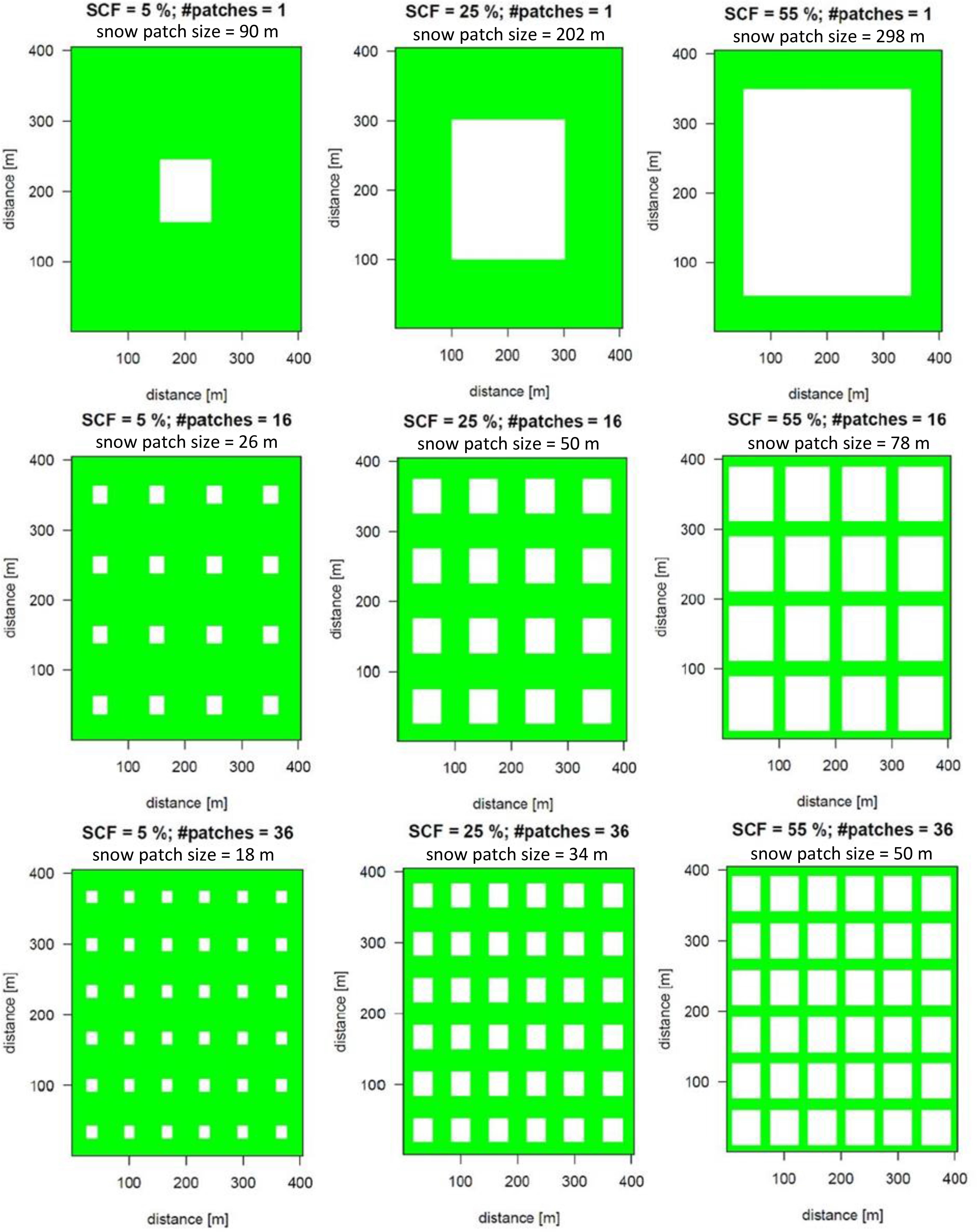
FIGURE 1. Initial idealized snow cover distributions, where the green colors indicate bare ground and white colors indicate snow. We choose a snow cover fraction (SCF) of 5, 25, and 55% and the number (#) of patches is equal to 1, 16, and 36. The snow patch size is additionally shown for each SCF and number of snow patches.

Model Setup

The physics-based surface process model Alpine3D has been used to simulate snow melt accounting for the patchiness of the snow cover. Alpine3D is a spatially distributed, three-dimensional model for analyzing and predicting dynamics of snow-dominated surface processes in mountainous topography (Lehning et al., 2006). In its standard version Alpine3D is limited to simulate pointwise the vertical turbulent exchange between the ground and the atmosphere and do not include lateral transport. Thus, the horizontal small scale variability in daily snow depth depletion rates (as observed from laser scanner measurements) could not be resolved (Mott et al., 2013). Air temperatures and wind velocity fields were calculated with the three-dimensional, non-hydrostatic atmospheric model ARPS (Advanced Regional Prediction System) (Xue et al., 2004). We used the 1.5-order turbulent kinetic energy scheme to parametrize the sub-grid scale turbulence (Deardorff, 1972). Turbulent fluxes were parametrized by using Monin–Obukhov bulk formulations and stability corrections of Deardorff (1972) in stable conditions. The radiative transfer model is given by Chou and Suarez (1994), which includes radiative cooling and forcing as well as topographical shading. The smaller time step was set to 0.001 s to integrate acoustic wave modes, the larger time step was set to 0.01 s to integrate the model. More details about the chosen setup in ARPS are described in detail in Mott et al. (2015).

Two-dimensional fields of snow cover distributions (Figure 1), aerodynamic roughness length and surface temperatures are used to initialize the base state of a force-restore land-surface soil-vegetation model (Noilhan and Planton, 1989). Vertical profiles of atmospheric variables (potential air temperature, relative air humidity, wind velocity, wind direction) are used to initialize the atmospheric base state of ARPS. ARPS was initialized with a neutral boundary layer assuming a potential air temperature of 295 K in all vertical levels. Relative air humidity (RH = 50%) and wind direction (WD = 315°) were assumed to be constant in all vertical levels. We chose a logarithmic wind profile for the initial model forcing. ARPS was run from 1^st April 06:00 to 18:00 local time for a clear-sky day in 2 m horizontal resolution. We used periodic boundary conditions in all directions, as this setup leads to less numerical instabilities than open (radiation) lateral boundary conditions. Numerical simulations were conducted for an initial ARPS surface temperature of the bare ground of 283.15 K and for three initial ARPS wind velocities (0.5, 2, and 5 m s^-1).

The spatial variability of air temperature and wind velocity fields induced by the patchiness of the snow cover is resolved by the atmospheric model. Thus heat is laterally transported from one grid point to the next in ARPS. Air temperature and wind velocity fields, generated with ARPS, are finally used as input for Alpine3D. Hence, the coupling of the two different models works only from the atmospheric model ARPS to the hydrological model Alpine3D and not vice versa.

In the physics-based surface process model Alpine3D, turbulent fluxes [sensible heat (H) and latent heat (Q_l )] were calculated with Monin–Obukhov bulk formulation by using the univariate stability corrections for momentum ψ_m and for scalars ψ_s according to Schlögl et al. (2017),

$$\mathrm{H}=\mathrm{C}\cdot \mathrm{\rho }\cdot {\mathrm{c}}_{\mathrm{p}}\cdot \overline{\mathrm{U}}\cdot \mathrm{\Delta }\mathrm{\theta },\mathrm{\hspace{0.17em}}\mathrm{\hspace{0.17em}}\mathrm{\hspace{0.17em}}\mathrm{\hspace{0.17em}}\mathrm{\hspace{0.17em}}\mathrm{\hspace{0.17em}}\mathrm{\hspace{0.17em}}\mathrm{\hspace{0.17em}}\mathrm{\hspace{0.17em}}\mathrm{\hspace{0.17em}}\mathrm{\hspace{0.17em}}\mathrm{\hspace{0.17em}}\mathrm{\hspace{0.17em}}\mathrm{\hspace{0.17em}}\mathrm{\hspace{0.17em}}\mathrm{\hspace{0.17em}}\mathrm{\hspace{0.17em}}\mathrm{\hspace{0.17em}}\mathrm{\hspace{0.17em}}\mathrm{\hspace{0.17em}}\mathrm{\hspace{0.17em}}(1)$$

where Δθ=θ_s-θ_zref is the potential air temperature difference, θ_zref is the virtual potential air temperature at the reference height z_ref, θ_s is the virtual potential temperature at the snow surface, $\overline{U}$ is the mean wind velocity and C is the exchange coefficient for stable conditions over snow,

$$C=\frac{k^2}{[\mathrm{ln(}\frac{z_{ref}}{z_{0}M})-{\mathrm{\psi }}_m]\cdot [\mathrm{ln(}\frac{z_{ref}}{z_{0}M})-{\mathrm{\psi }}_s],}\mathrm{\hspace{0.17em}}\mathrm{\hspace{0.17em}}\mathrm{\hspace{0.17em}}\mathrm{\hspace{0.17em}}\mathrm{\hspace{0.17em}}\mathrm{\hspace{0.17em}}\mathrm{\hspace{0.17em}}\mathrm{\hspace{0.17em}}\mathrm{\hspace{0.17em}}\mathrm{\hspace{0.17em}}\mathrm{\hspace{0.17em}}\mathrm{\hspace{0.17em}}\mathrm{\hspace{0.17em}}\mathrm{\hspace{0.17em}}\mathrm{\hspace{0.17em}}\mathrm{\hspace{0.17em}}\mathrm{\hspace{0.17em}}\mathrm{\hspace{0.17em}}\mathrm{\hspace{0.17em}}\mathrm{\hspace{0.17em}}\mathrm{\hspace{0.17em}}\mathrm{\hspace{0.17em}}\mathrm{\hspace{0.17em}}\mathrm{\hspace{0.17em}}\mathrm{\hspace{0.17em}}\mathrm{\hspace{0.17em}}(2)$$

where k = 0.4 is the von Kármán constant and z_(0M) = 0.007 m is the aerodynamic surface roughness length over snow (Bavay et al., 2009; Schlögl et al., 2016). For bare ground, we chose alpine meadow with a surface roughness length of 0.03 m according to Wieringa (1993).

The full surface energy balance and the melt energy for snow (Q_m ) were calculated in Alpine3D for one day from 6:00 to 18:00 by forcing the model with ARPS meteorological fields each 15 min:

$$Q_m=SW\mathrm{\hspace{0.17em}}\downarrow -SW\mathrm{\hspace{0.17em}}\uparrow +LW\mathrm{\hspace{0.17em}}\downarrow -LW\mathrm{\hspace{0.17em}}\uparrow +H+O_l.\mathrm{\hspace{0.17em}}\mathrm{\hspace{0.17em}}\mathrm{\hspace{0.17em}}\mathrm{\hspace{0.17em}}\mathrm{\hspace{0.17em}}\mathrm{\hspace{0.17em}}\mathrm{\hspace{0.17em}}\mathrm{\hspace{0.17em}}\mathrm{\hspace{0.17em}}\mathrm{\hspace{0.17em}}\mathrm{\hspace{0.17em}}\mathrm{\hspace{0.17em}}\mathrm{\hspace{0.17em}}\mathrm{\hspace{0.17em}}\mathrm{\hspace{0.17em}}\mathrm{\hspace{0.17em}}\mathrm{\hspace{0.17em}}\mathrm{\hspace{0.17em}}\mathrm{\hspace{0.17em}}\mathrm{\hspace{0.17em}}\mathrm{\hspace{0.17em}}\mathrm{\hspace{0.17em}}\mathrm{\hspace{0.17em}}\mathrm{\hspace{0.17em}}\mathrm{\hspace{0.17em}}\mathrm{\hspace{0.17em}}\mathrm{\hspace{0.17em}}(3)$$

Radiation components (incoming shortwave radiation SW ↓, outgoing shortwave radiation SW ↑ incoming longwave radiation LW ↓ and outgoing longwave radiation LW ↑) were selected from a clear-sky day of beginning of April at a test site with an elevation of 2000 m asl. The incoming longwave radiation is parametrized with a clear-sky algorithm of Dilley and O’Brien (1998) in combination with the cloud correction algorithm of Unsworth and Monteith (1975). This setup allows changes in the incoming longwave radiation due to changes in the air temperatures. Incoming and outgoing shortwave radiation are measured and avoid a model-based snow surface albedo estimation.

In the following we focus on snow depth depletion rates ΔHS=HS_18:00-HS_06:00 instead of the melt energy for snow Q_m , in order to compare numerical results with snow depth depletion rates recorded from terrestrial laser scanning in the companion paper. The conversion from Q_m to ΔHS is done for each model pixel by the physics-based surface process model SNOWPACK (Lehning et al., 2002), which is the physical core of the Alpine3D model.

Model Setup for the Wannengrat Test Site

Numerical results of the idealized flat test site have been compared with numerical results for the test site Wannengrat, Davos, Switzerland (Mott et al., 2015). The Wannengrat test site has been mapped on a regular grid with a horizontal resolution of 5 m and includes 547 × 579 pixels with an elevation between 2069 and 2647 m asl. The average slope angle of the Wannengrat test site is 19° with a standard deviation of 10°. More detailed information about the Wannengrat test site can be found in Mott et al. (2015). ARPS was initialized with measured snow distributions recorded with terrestrial laser scanning at the Wannengrat test site. Meteorological fields of air temperature and wind velocity are calculated in ARPS for SCF = 15, 23, 37, 50, and 65% and one quiescent (0 m s^-1) and one synoptic forcing (3 m s^-1).

Open (radiation) boundary conditions and an integration time of 700 s have been used for the Wannengrat test site, as the model becomes numerical unstable afterward. The model was initialized for 12:00 local time for a clear sky day. In order to compare both test sites (see section “Comparison of the Idealized Test Site With the Wannengrat Test Site”), the Wannengrat specific model setup is additionally used for the idealized test site.

Procedure

We analyzed ARPS meteorological fields and Alpine3D turbulent sensible heat fluxes and daily snow depth depletion rates for seven different initial conditions. We modified the SCF (5, 25, and 55%), the number of snow patches (1, 16, and 36) and the wind velocity (0.5, 2, and 5 m s^-1). Additionally, we simulated one continuous snow cover with a wind velocity of 2 m s^-1 (Table 1). We calculated ARPS meteorological fields for the model level at z_ref =0.8 m above the surface and a model level at z_ref =5.7 m above the surface. By analyzing ARPS meteorological fields for both model levels, we investigate a potential bias by using standard input meteorological stations which typically provide measurements between 2 and 10 m above the surface and only record spatially averaged values of atmospheric fields from a heterogeneous land surface.

TABLE 1

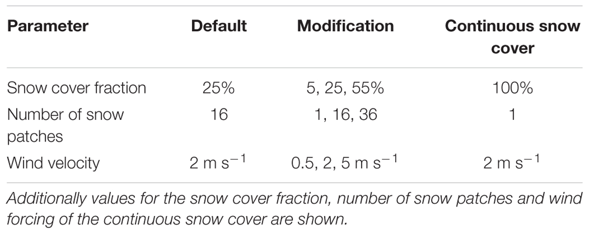
TABLE 1. Default values and their modifications of the initial wind velocity and the snow distributions (snow cover fraction and number of patches) are shown.

The variation in near-surface air temperatures ΔT_a, turbulent sensible heat fluxes ΔH and snow depth depletion rates Δ(ΔHS) of the seven model simulations are calculated with respect to the simulation of the continuous snow cover (csc):

${\mathrm{\Delta }T}_a=T_{a,sim}-T_{a,\csc }\left(4\mathrm{a}\right)$

$\mathrm{\Delta }H=H_{sim}-H_{\csc }\left(4\mathrm{b}\right)$

$\mathrm{\Delta }\left(\mathrm{\Delta }HS\right)=\mathrm{\Delta }H{S}_{sim}-\mathrm{\Delta }H{S}_{\csc }\left(4\mathrm{c}\right)$

The variation in near-surface ARPS air temperatures ΔT_a are compared with results from the temperature footprint approach in the companion paper. The temperature footprint approach is developed from adapted footprint estimations (Schuepp et al., 1990) in order to resolve the spatial variability of near-surface air temperatures and turbulent sensible heat fluxes. This fundamental theory was originally deployed for eddy-covariance measurements revealing the origin of the measured turbulence as a function of the measurement height, atmospheric stability, and wind speed.

Results

Variation of Atmospheric Fields

Advanced Regional Prediction System air temperature and wind velocity fields are simulated for two different heights above the ground as a function of the local time (Figure 2). Air temperatures in the lowest model level decrease in the first time step about 1 K indicating that the base-state potential air temperature of 295 K and the surface are not in equilibrium. Afterward, air temperatures increase with sunrise, strongly for the near-surface model level but also for the model level at 5.7 m above the surface. The near-surface air temperature increase is heavily dependent on the chosen wind conditions and snow distributions (Figure 3).

FIGURE 2

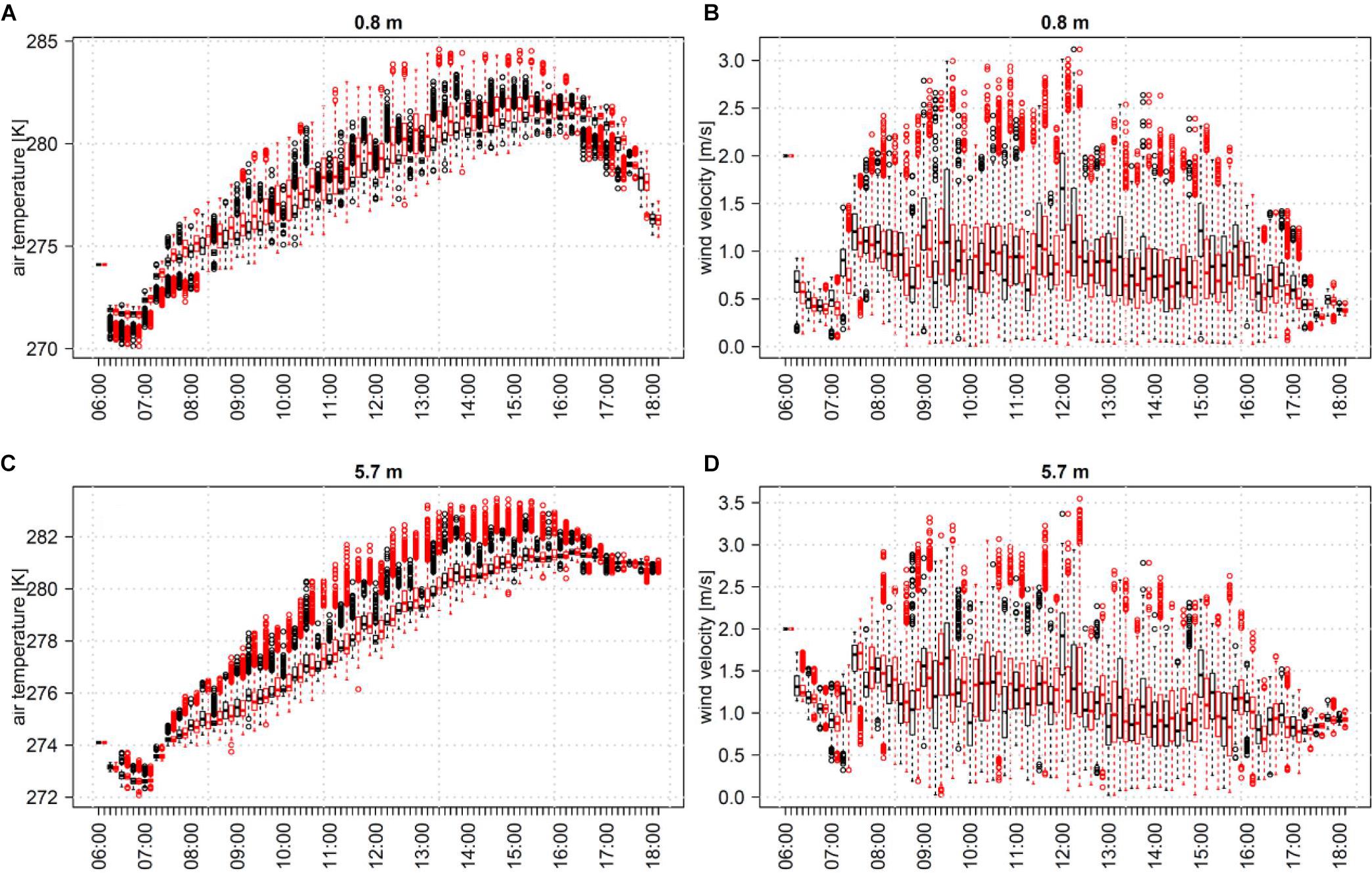
FIGURE 2. Development of the diurnal ARPS air temperature in 0.8 m (A) and 5.7 m (C) above the surface for SCF = 25% and a number of snow patches = 16. Development of the diurnal ARPS wind velocity in 0.8 m (B) and 5.7 m (D) above the surface for SCF = 25% and a number of snow patches = 16. Initial values for the wind velocity are 2 m s^-1 and temperature of the adjacent bare ground is 283.15 K. Results are shown as boxplots for snow-covered pixels (black) and all pixels (red) as a function of the local time.

FIGURE 3

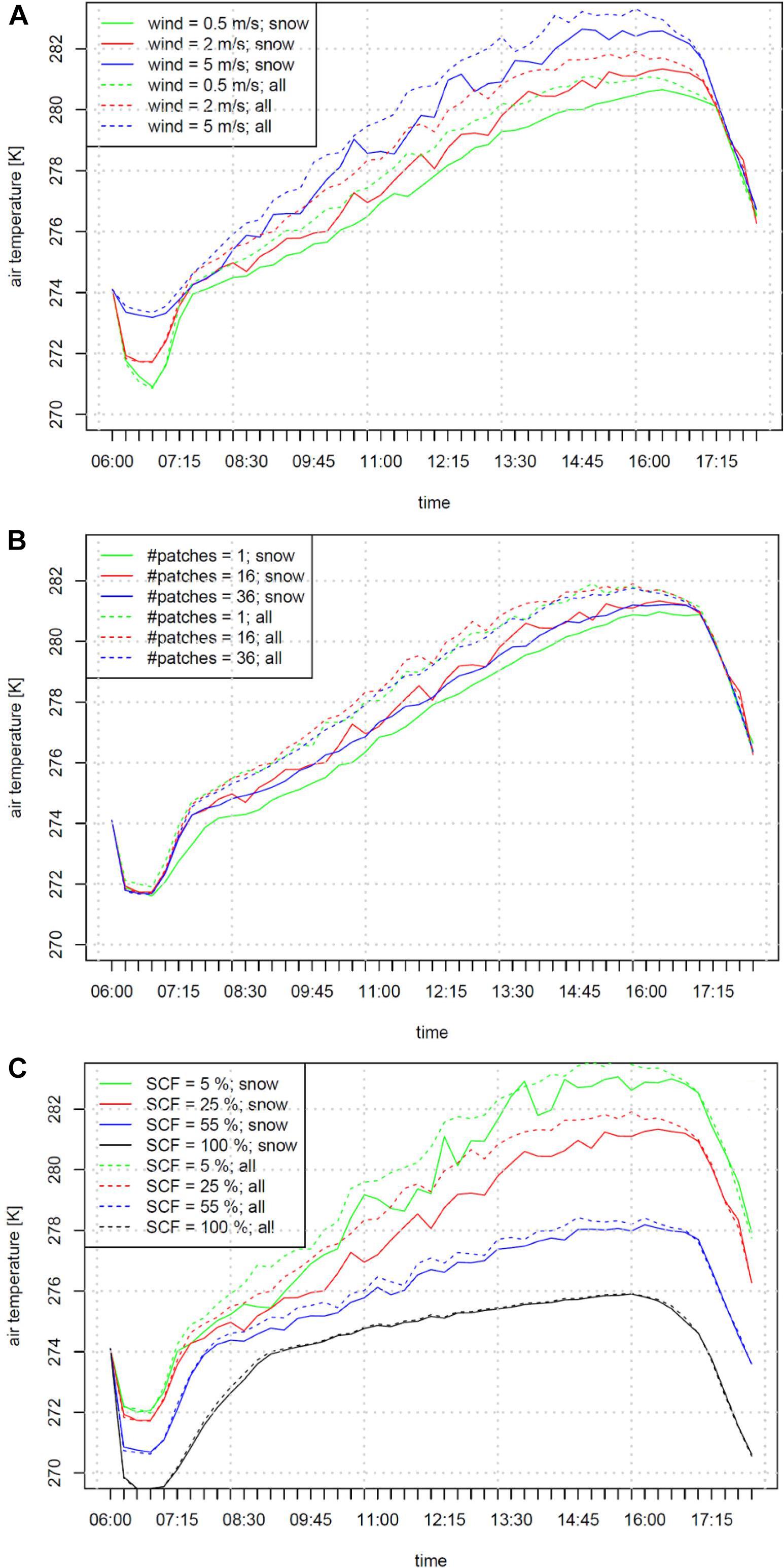
FIGURE 3. Development of the diurnal mean air temperature [K] for a set of different wind velocities (0.5, 2, 5 m s^-1) (A), for a set of a different number of snow patches (1, 16, 36) (B) and for a set of different SCF (5, 25, 55, 100%) (C). The default values are SCF = 25%, number of snow patches = 16 and wind velocity = 2 m s^-1.

Over snow covered pixels, daily averaged near-surface air temperatures increase around ΔT_a =1.8 ± 0.4 K (3.7 ± 0.5 K, 4.9 ± 0.5 K) by lowering the SCF from a continuous snow cover to 55 (25, 5) % (Figure 3C). For SCF = 25%, the lowest ARPS near-surface air temperatures are found for small initial wind velocities. Near-surface air temperatures exceed 280 K for a calm wind forcing (0.5 m s^-1) at 15:00 local time (ΔT_a = 3.2K). Near-surface air temperatures increase to 282 K (ΔT_a = 4.8K) for a synoptic wind forcing (5 m s^-1) (Figure 3A). ARPS near-surface air temperatures are not sensitive to variations in the number of snow patches. For SCF = 25%, we found the smallest near-surface air temperatures for one large snow patch and the largest near-surface air temperatures for many smaller snow patches, but differences are smaller than 0.5 K (Figure 3B). We additionally modified initial soil temperatures of the adjacent bare ground from 278 to 288 K. Near-surface air temperatures slightly increase with increasing soil temperatures, but numerical results are insensitive to modifications in the soil temperature as differences are smaller than 0.5 K (not shown).

Air temperatures at 0.8 and 5.7 m for snow-covered pixels are almost similar from sunrise until sunset. However, air temperatures close to the snow surface rapidly decrease after sunset, whereas air temperatures higher up in the atmosphere are less affected by the cooling snow surface and stay almost constant in the first hour after sunset. In summary, variations between both vertical levels can be neglected as long as the energy balance of the snow pack remains positive (Q_m > 0)) and the surface temperature consistently stays at its melting point.

The air temperatures differences between the model level in 0.8 and 5.7 m above surface for snow-covered pixels are shown as a function of the fetch distance and local time (Figure 4). Warm air advection influences the snow covered pixels with a fetch distance lower than 5–10 m in the lowermost model level. The hourly variations in air temperature differences for small fetch distances explain the variations in Figure 3C for small SCFs. As the relative percentage of small fetch distances is small for a large fraction of snow, the curves in Figure 3C are smoothed for a large fraction of snow.

FIGURE 4

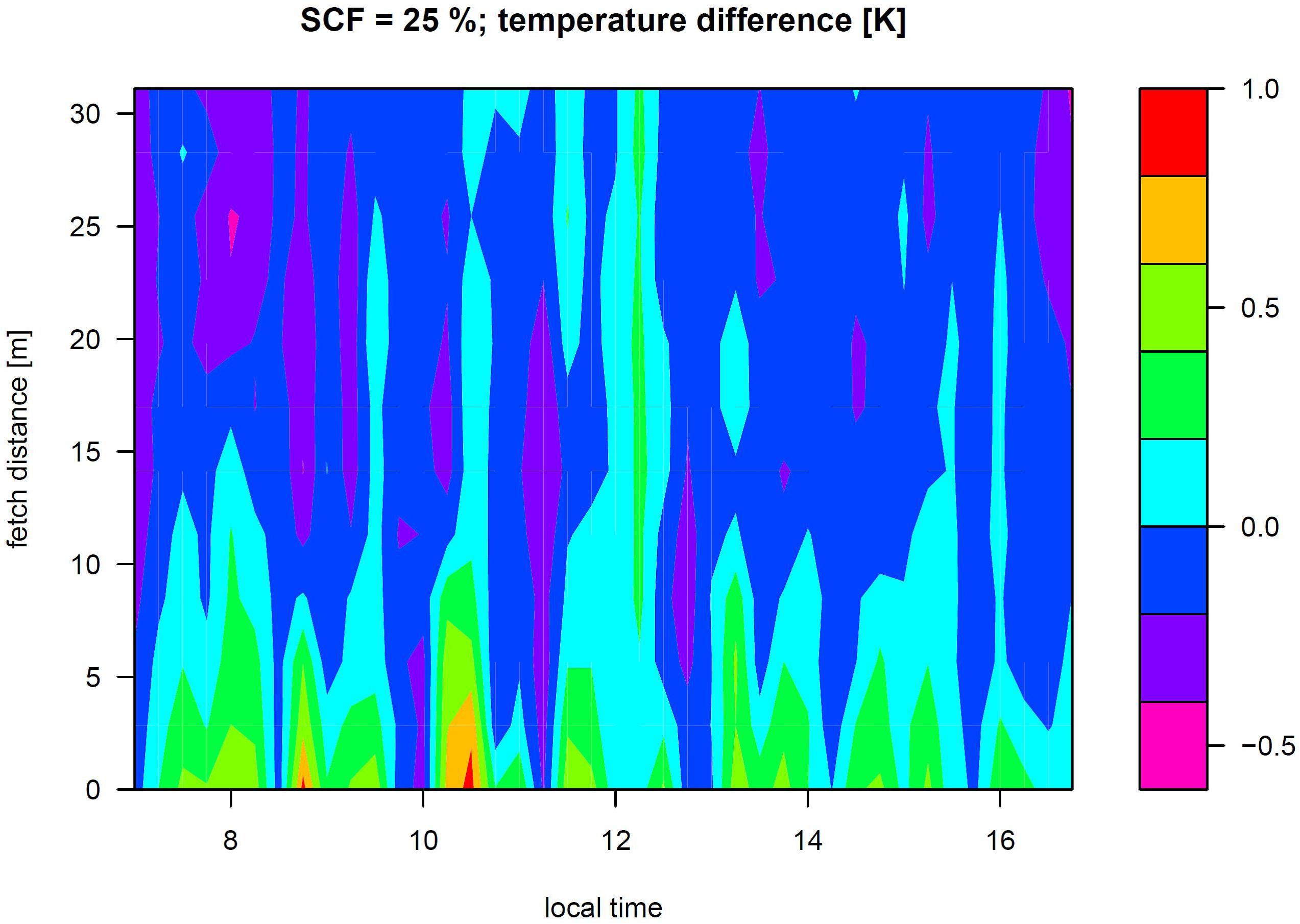
FIGURE 4. Temperature difference [K] between the lowest model level (0.8 m) and the model level in 5.7 m as a function of the local time and the fetch distance [m] for a SCF = 25% and a wind velocity of 2 m s^-1. Positive values indicate warmer temperatures in 0.8 m above the surface than in 5.7 m above the surface.

Air temperatures for snow-covered pixels and all pixels are similar at 5.7 m above the surface. However, near-surface air temperatures for all pixels are up to 1 K larger than for only snow-covered pixels. This difference increases with decreasing SCF caused by the fact that smaller snow-covered areas lead to less cooling of the lowermost model level than a land surface with a larger fraction of snow.

Accurate wind velocity fields are required to calculate Alpine3D surface turbulent sensible heat fluxes and snow depth depletion rates correctly. ARPS wind velocities increase with sunrise, stay constant throughout the day and decrease with sunset. Wind velocities for the lowermost model level are smaller than higher up in the atmosphere, especially in the morning. Turbulent mixing of air masses becomes more important with increasing air temperatures after sunrise, leading to small differences in wind velocities between both model levels (0.8 vs. 5.7 m) during noon.

We analyzed the correlation between ARPS air temperature and wind velocity fields close to the snow surface for snow-covered pixels. For a synoptic forcing (5 m s^-1), we found a strong negative correlation mainly attributed to a change in the aerodynamic roughness length at the transition between the rougher snow-free ground and the smoother snow patch. Close to the ground-snow transition, air temperatures are 1–2 K larger than further inside the snow patch, whereas wind velocities are slightly smaller at the upwind edge of the snow patch than further inside the snow patch. This increase in wind velocity over the snow patch in downwind direction was not yet observed experimentally and explains that daily averaged wind velocities over snow decrease approximately 10% by decreasing the SCF from a continuous snow cover to 5%. For calm wind conditions (0.5 m s^-1), the formation of a snow-breeze circulation favors a low-level jet at the border between snow and bare ground in our numerical simulations. This phenomenon leads to a decrease in wind velocities in downwind direction and therefore a weak positive correlation between wind velocity and air temperature fields.

Turbulent Sensible Heat Fluxes and Snow Depth Depletion Rates

In this section, we investigate the sensitivity of surface turbulent sensible heat fluxes (Figure 5) and daily snow depth depletion rates (Table 2) to different initial wind conditions and snow cover distributions. Surface turbulent sensible heat fluxes typically show larger negative values by using air temperature and wind velocity fields at 0.8 m instead of meteorological fields at 5.7 m (mean turbulent sensible heat fluxes for all simulations: 16 W m^-2 at 0.8 m vs. 6 W m^-2 at 5.7 m), which is discussed in detail in Section “Discussion and Conclusion.” The largest turbulent sensible heat fluxes occur at around 15:00 local time for our specific example of 1^st April, where air temperatures typically reach the daily maximum, and decrease afterward in strong correlation with the air temperatures. The standard deviation of the turbulent sensible heat fluxes is largest at around 13:00 local time and increase with decreasing SCF and increasing wind velocity (Figure 6). In the following we present the Alpine3D surface energy balance for varying SCFs, initial wind velocities and number of snow patches:

FIGURE 5

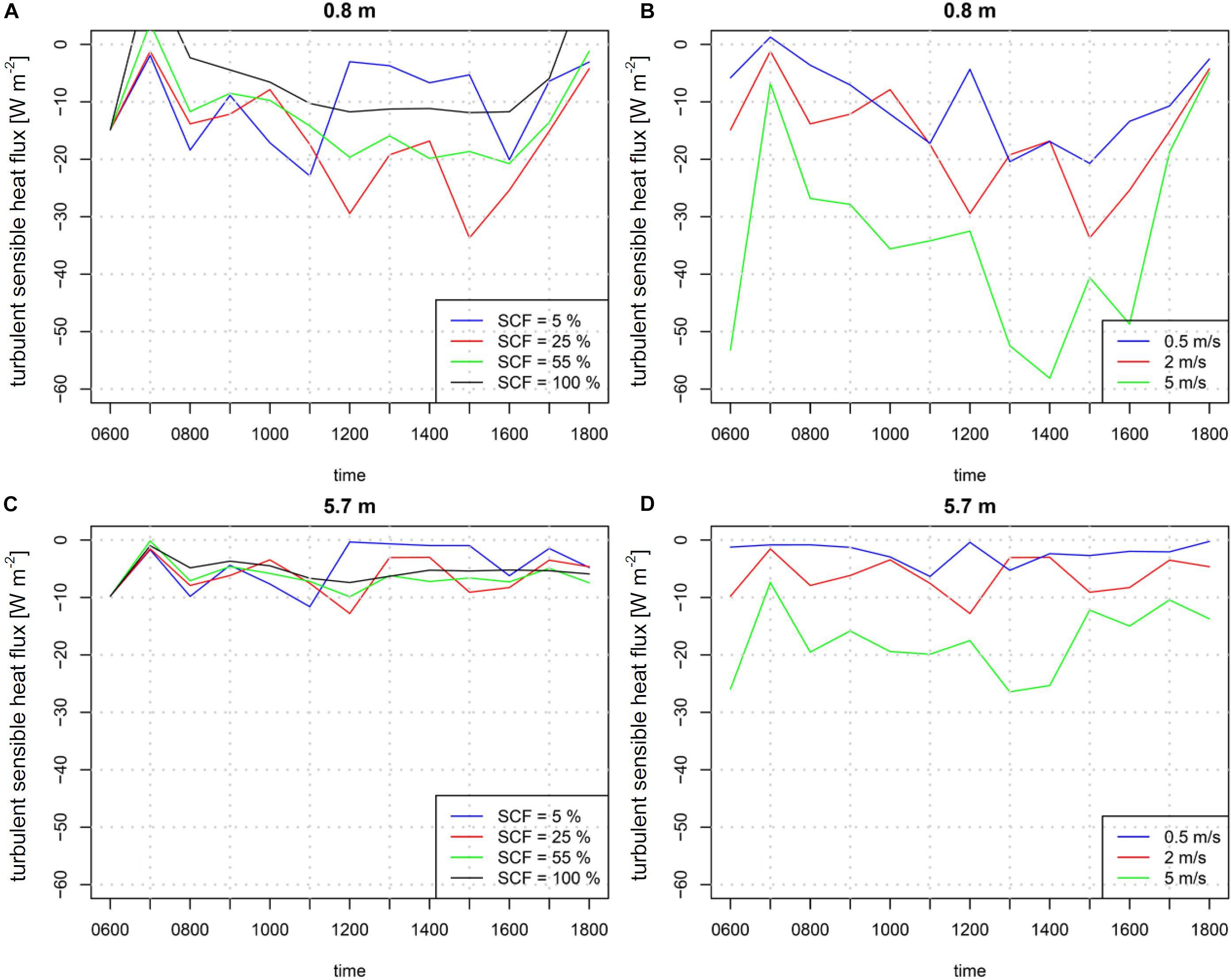
FIGURE 5. Surface turbulent sensible heat flux over snow [W m^-2] as a function of the local time by using ARPS meteorological fields of the near-surface model level (0.8 m, A,B) and a model level higher up in the atmosphere (5.7 m, C,D). Simulations with varying SCF (A,C) and varying initial wind velocity (B,D) are shown.

TABLE 2

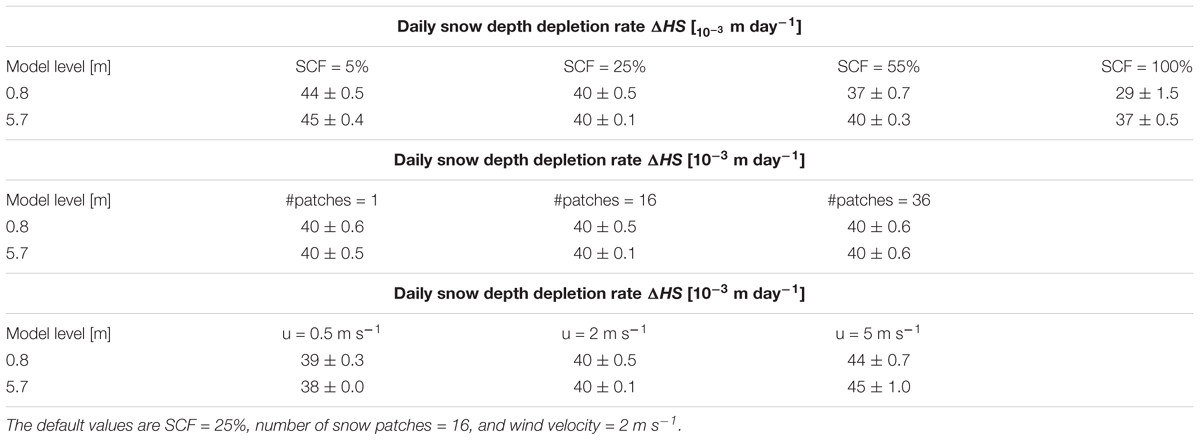
TABLE 2. Daily snow depth depletion rates ΔHS [10^-3m day^-1] as a function of snow cover fraction (upper table), number of snow patches (middle table) and wind forcing (lower table).

FIGURE 6

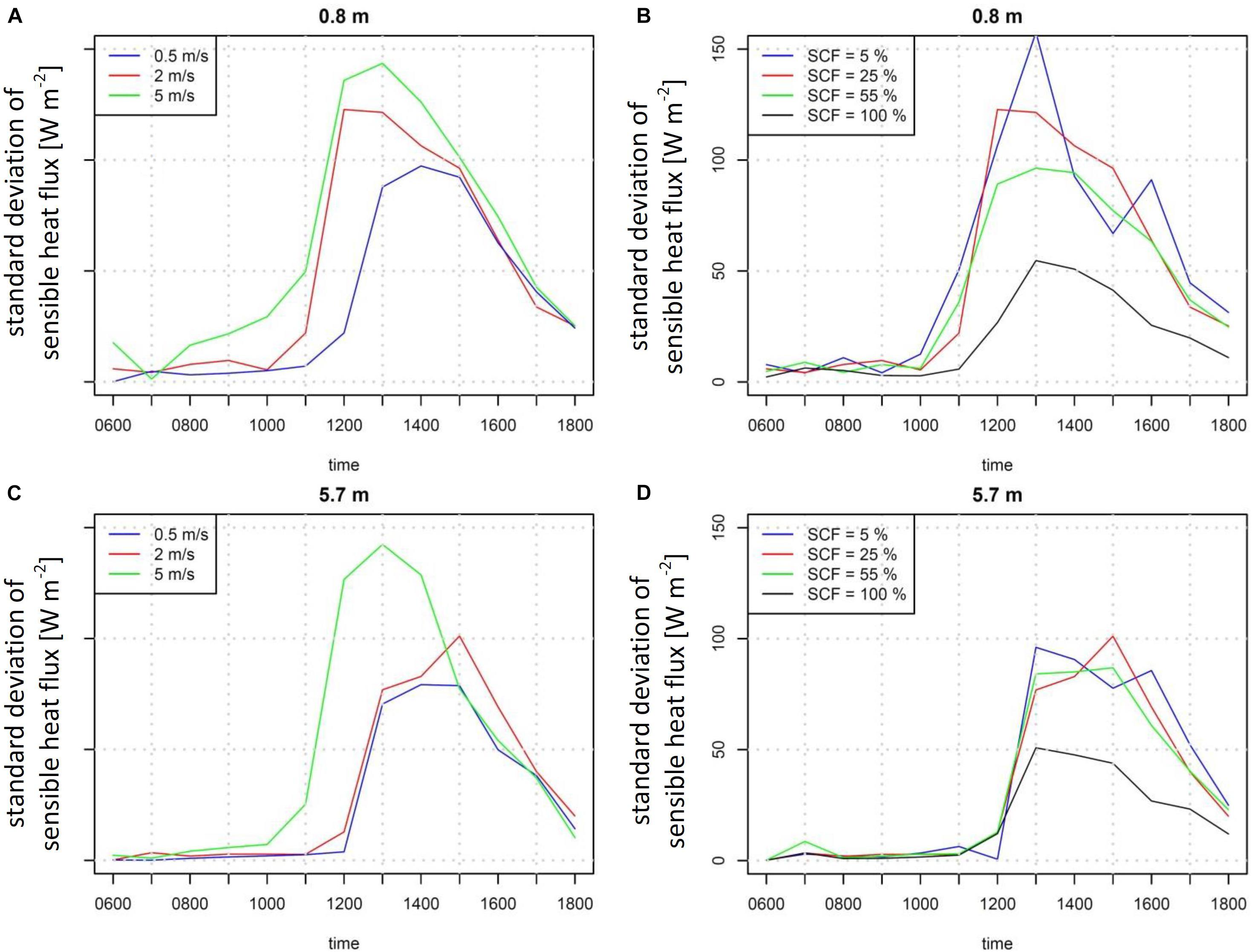
FIGURE 6. Standard deviation of the surface turbulent sensible heat flux over snow [W m^-2] as a function of the local time by using ARPS meteorological fields of the near-surface model level (0.8 m, A,B) and a model level higher up in the atmosphere (5.7 m, C,D). Simulations with varying SCF (A,C) and varying initial wind velocity (B,D) are shown.

(1) Snow cover fraction: A varying fraction heavily affects surface turbulent sensible heat fluxes and daily snow depth depletion rates. The largest snow depth depletion rates were simulated for a SCF = 5%, as ARPS air temperatures and surface turbulent sensible heat fluxes are largest for this model setup. By using near-surface meteorological fields, daily snow depth depletion rates increase from 29 × 10^-3 m day^-1 to 44 × 10^-3 m day^-1 by varying the snow distribution from an almost continuous snow cover to SCF = 5%. For SCF = 55%, snow depth depletion rates are significantly larger by using meteorological fields at 5.7 m above the surface instead of near-surface meteorological fields (37 × 10^-3 vs. 40 × 10^-3 m day^-1). This is mostly caused by the formation of a stable internal boundary layer in the model and a cooling of near-surface air temperatures by the presence of the snow. This cooling of the near-surface atmosphere could also be observed for the continuous snow cover (initial wind velocity = 2 m s^-1), where daily snow depth depletion rates are 25% smaller by using near-surface meteorological fields as model input (29 × 10^-3 vs. 37 × 10^-3 m day^-1).

(2) Initial wind velocity: For a synoptic forcing (wind velocity = 5 m s^-1), surface turbulent sensible heat fluxes are large throughout the day (up to 60 W m^-2), whereas surface turbulent sensible heat fluxes are small (up to 20 W m^-2) for calm conditions (wind velocity = 0.5 m s^-1). This surface reaction to the decrease in the initial wind velocity is then represented in daily snow depth depletion rates, which slightly decrease from 44 to 39 × 10^-3 m day^-1. The Alpine3D surface energy balance show similar results for the usage of meteorological fields at 0.8 and 5.7 m above the surface.

(3) Number of snow patches: The sensitivity of turbulent sensible heat fluxes and daily snow depth depletion rates to modifications in the number of snow patches is small. Differences in the surface energy balance are small by using ARPS meteorological fields in different heights.

On average, daily snow depth depletion rates are around 40% larger for a patchy snow cover with SCF = 5% in comparison with a continuous snow cover (Table 3). This large difference is mainly caused by an increase in mean air temperatures causing an increase in surface turbulent sensible heat fluxes from 5 W m^-2 for a continuous snow cover to 15 W m^-2 for a SCF = 5%. For SCF = 55%, we analyzed an increase in surface turbulent sensible heat fluxes of 73%, which leads to 22% larger snow depletion rates in comparison with a continuous snow cover.

TABLE 3

TABLE 3. Daily mean ΔH [W m^-2] and Δ(ΔHS) [10^-3 m day^-1] by using meteorological fields close to the snow surface for different snow cover fraction, a wind velocity of 2 m s^-1 and the number of snow patches = 16 relative to a continuous snow cover.

We investigated turbulent sensible heat fluxes and snow depth depletion rates as a function of the fetch distance. The small horizontal small-scale variability in near-surface air temperature fields of ARPS leads to almost constant turbulent sensible heat fluxes and snow depth depletion rates throughout the snow patch. For synoptic forcing situations, ARPS near-surface air temperatures are 1–2 K larger at the leading edge of the snow patches than further inside of the snow patch. For calm conditions, ARPS near-surface air temperatures are only 0.5 K larger at the leading edge of snow patches. Therefore, the “leading edge effect” in daily snow depth depletion rates as recorded with the laser scanner could not sufficiently be resolved and possible reasons will be discussed in Section “Discussion and Conclusion.”

Comparison of the Idealized Test Site With the Wannengrat Test Site

We compared surface turbulent sensible heat fluxes between the idealized flat test site and the Wannengrat test site (Figure 7). Numerical findings of the surface energy balance for the idealized test site are in a similar range as results for the Wannengrat test site. However, we found significant differences in surface turbulent sensible heat fluxes between both test sites, as slope-induced atmospheric processes become significant in complex terrain. Hence, the variation of surface turbulent sensible heat fluxes due to different SCF is larger in complex terrain. The development of katabatic flows was observed for a quiescent forcing and lead to a decrease of turbulent sensible heat fluxes with a decreasing fraction of snow (Mott et al., 2015). In contrast, surface turbulent sensible heat fluxes increase with decreasing SCF for the idealized flat test site for a quiescent forcing as described in detail in Section “Turbulent Sensible Heat Fluxes and Snow Depth Depletion Rates.”

FIGURE 7

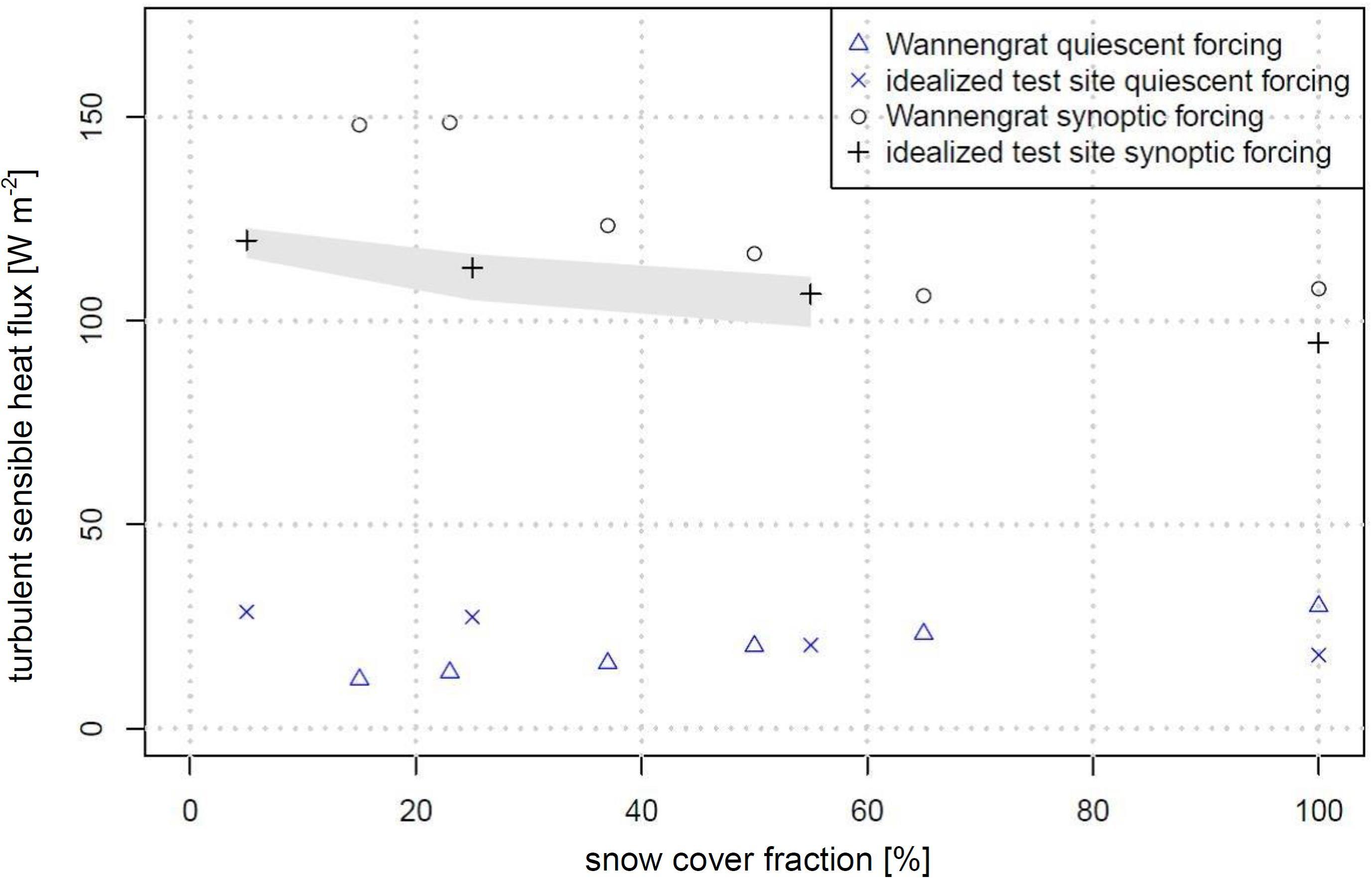
FIGURE 7. Surface turbulent sensible heat flux over snow [W m^-2] as a function of the SCF for the idealized test site and the Wannengrat test site for a quiescent (blue) and synoptic forcing (black). The shaded area for the synoptic forcing of the idealized test site represents the uncertainty caused by the different number of snow patches.

For a synoptic forcing, surface turbulent sensible heat fluxes over snow increase for the idealized test site and the Wannengrat test site with a decreasing fraction of snow. However, the sensitivity of surface turbulent sensible heat fluxes to the SCF is weaker for the idealized test site than for the Wannengrat test site caused by the fact that ARPS near-surface air temperatures und wind velocities are negatively correlated for the idealized test site, which leads to a damping of surface turbulent sensible heat fluxes. For the Wannengrat test site, however, the strong negative correlation was not observed, as changes in the wind velocity due to changes in the aerodynamic roughness length are less dominant than thermally-driven horizontal small-scale variations in the wind velocity field.

Discussion and Conclusion

We showed that patchy snow covers significantly alter the surface energy balance of a snow pack. Once the snow cover gets patchy and the SCF decreases to 55% (25 and 5%), the mean air temperature significantly increases ΔT_a =1.8 K (3.7 and 4.9 K) leading to a significant increase in daily mean snow depth depletion rates Δ(ΔHS) =22% (33 and 40%). The sensitivity of daily snow depth depletion rates to varying snow distributions is mostly caused by a positive snow-albedo feedback which leads to an increase in mean air temperatures with a decreasing fraction of snow stimulating an increasing heat exchange toward the snow cover.

The small-scale variability of near-surface air temperatures at the first ARPS model level (0.8 m) is around one order of magnitude smaller than results from the temperature footprint approach, where near-surface air temperatures are calculated at a height of 0.01 m above the surface. This difference in the small-scale variability of near-surface air temperatures could be explained by the different height above ground. Alpine3D is not able to resolve the “leading-edge effect” (as recorded with the laser scanner) by forcing the model with ARPS meteorological fields at 0.8 m above the surface. Our model resolution for this study is already much higher than usual for a meteorological model. Increasing the resolution even more will not be practical for real-world applications such as in hydrology or meteorology due to computational limitations.

Figure 8 compares the mean air temperature increase averaged over snow-covered pixels between ARPS model results and the temperature footprint approach as a function of the SCF and wind velocity. Although ARPS could not sufficiently resolve the leading-edge effect, the mean air temperature increase averaged over snow-covered pixels (and hence the additional energy due to lateral transport processes) is similar for a large range of snow patch distributions and meteorological conditions. The correlation coefficient between the temperature footprint approach and ARPS model results is larger for the near-surface model level at 0.8 m than for the model level at 5.7 m above the surface. Differences in values of the mean air temperature increase between both approaches are large for a calm wind forcing (0.5 m s^-1), which could be explained by the fact that the formation of a stable internal boundary layer is not fully resolved for the ARPS model simulation with a calm wind forcing and a SCF = 25%.

FIGURE 8

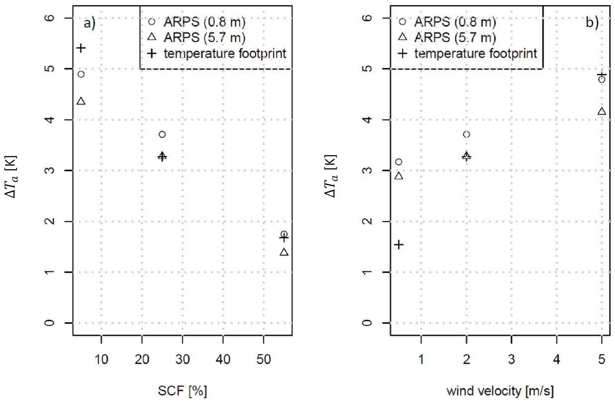
FIGURE 8. ΔT_a [K] over snow as a function of the SCF [%] (a) and wind velocity [m s^-1] (b) for the usage of ARPS meteorological fields in 0.8 and 5.7 m above the surface and for the temperature footprint approach. The default values are SCF = 25%, number of snow patches = 16, and wind velocity = 2 m s^-1.

We investigated differences in surface turbulent sensible heat fluxes by using meteorological fields in different heights above the surface (Figure 3). For idealized conditions (e.g., continuous land surface, constant flux layer), the Monin–Obukhov bulk formulation predicts identical surface turbulent sensible heat fluxes if meteorological fields in different measurement heights are used. However, idealized conditions, which are required for the application of Monin–Obukhov bulk formulation, are heavily violated for patchy snow covers and the developing internal boundary layers of small vertical extent. Therefore, Monin–Obukhov formulations with the stability corrections, which are typically developed for situations with a continuous snow cover (Schlögl et al., 2017), could not account for the specific conditions over patchy snow covers, where strongly turbulent, warm air masses (originating from the adjacent bare ground) were advected toward snow patches with highly different surface characteristics. This warm air advection leads to very large temperatures differences over a short vertical distance, resulting in a very stable atmosphere directly above the snow surface. Schlögl et al. (2017) showed that stability corrections for a very stable atmosphere already show large errors over a continuous snow cover. Hence, surface turbulent sensible heat fluxes over patchy snow covers could strongly differ and will give erroneous estimations of the true surface heat exchange when using meteorological fields in different heights above the surface especially if the height of the stable internal boundary layer is located close to the ground. The difference in turbulent sensible heat fluxes could be interpreted as the model uncertainty over patchy covers by violating necessary requirements in the Monin–Obukhov bulk formulation.

Our results have shown that knowledge about the snow cover distribution is a necessary requirement to correctly assess the additional energy to the surface energy balance from lateral transport processes of heat, momentum, and moisture. Snow cover distributions are heavily dependent on different terrain parameters (Moore et al., 1991) of the digital elevation model. A patchy snow cover typically has a large mean snow patch size for a small horizontal scale of local depressions in the digital elevation model. The mean snow patch size decreases when the horizontal scale of local depressions increases. A parametrization of a patchy snow cover distribution on a very small scale as a function of different terrain parameters would be complementary to the study of Helbig et al. (2015), where snow covered areas on larger scales up to 3 km were parametrized.

We tested the sensitivity of major numerical results to varying initial wind velocities. A sensitivity analysis with respect to varying aerodynamic roughness lengths for both snow and bare ground, cloud cover, the horizontal resolution of the model grid, time of the year and parametrizations of stability corrections and incoming longwave radiation, goes beyond the scope of this study, but will be addressed in a future work.

Author Contributions

SS conducted the analysis and wrote the manuscript. ML and RM conceived and supervised the project, provided guidance, helped with the analysis, and revised the manuscript.

Funding

The work was funded by Swiss National Science Foundation (Project: Snow-atmosphere interactions driving snow accumulation and ablation in an Alpine catchment: The Dischma Experiment; SNF-Grant: 200021_150146 and Project: The sensitivity of very small glaciers to micrometeorology. P300P2_164644).

Conflict of Interest Statement

The authors declare that the research was conducted in the absence of any commercial or financial relationships that could be construed as a potential conflict of interest.

References

Bavay, M., Lehning, M., Jonas, T., and Löwe, H. (2009). Simulations of future snow cover and discharge in alpine headwater catchments. Hydrol. Process. 23, 95–108. doi: 10.1002/hyp.7195

CrossRef Full Text | Google Scholar

Chou, M. D., and Suarez, M. J. (1994). An efficient thermal infrared radiation parameterization for use in general circulation models. NASA Tech. Memo. Server 3:85.

Google Scholar

Deardorff, J. W. (1972). Numerical investigation of neutral and unstable planetary boundary layers. J. Atmos. Sci. 29, 91–115. doi: 10.1175/1520-0469(1972)029<0091:NIONAU>2.0.CO;2

CrossRef Full Text

Dilley, A. C., and O’Brien, D. M. (1998). Estimating downward clear sky long-wave irradiance at the surface from screen tem-perature and precipitable water. Q. J. R. Meteorol. Soc. 124, 1391–1401. doi: 10.1002/qj.49712454903

CrossRef Full Text | Google Scholar

Egli, L., Jonas, T., Grünewald, T., Schirmer, M., and Burlando, P. (2012). Dynamics of snow ablation in a small alpine catchment observed by repeated terrestrial laser scans. Hydrol. Process. 26, 1574–1585. doi: 10.1002/hyp.8244

CrossRef Full Text | Google Scholar

Essery, R., Granger, R., and Pomeroy, J. (2006). Boundary-layer growth and advection of heat over snow and soil patches: modelling and parameterization. Hydrol. Process. 20, 953–967. doi: 10.1002/hyp.6122

CrossRef Full Text | Google Scholar

Essery, R., Morin, S., Lejeune, Y., and Menard, C. B. (2013). A comparison of 1701 snow models using observations from an alpine site. Adv. Water Resour. 55, 131–148. doi: 10.1016/j.advwatres.2012.07.013

CrossRef Full Text | Google Scholar

Fujita, K., Hiyama, K., Iida, H., and Ageta, Y. (2010), Self-regulated fluctuations in the ablation of a snow patch over four decades. Water Resour. Res. 46, W11541. doi: 10.1029/2009WR008383

CrossRef Full Text

Garratt, J. R. (1990). The internal boundary layer – A review. Boundary Layer Meteorol. 50, 171–203. doi: 10.1007/BF00120524

CrossRef Full Text | Google Scholar

Gerber, F., Lehning, M., Hoch, S. W., and Mott, R. (2017). A close-ridge small-scale atmospheric flow field and its influence on snow accumulation. J. Geophys. Res. Atmos. 122, 7737–7754. doi: 10.1002/2016JD026258

CrossRef Full Text | Google Scholar

Granger, R. J., Essery, R., and Pomeroy, J. W. (2006). Boundary-layer growth over snow and soil patches: field observations. Hydrol. Process. 20, 943–951. doi: 10.1002/hyp.6123

CrossRef Full Text | Google Scholar

Granger, R. J., Pomeroy, J. W., and Parviainen, J. (2002). Boundary-layer integration approach to advection of sensible heat to a patchy snow cover. Hydrol. Process. 16, 3559–3569. doi: 10.1002/hyp.1227

CrossRef Full Text | Google Scholar

Groot Zwaaftink, C. D., Löwe, H., Mott, R., Bavay, M., and Lehning M. (2011). Drifting snow sublimation: a high-resolution 3-D model with temperature and moisture feedbacks. J. Geophys. Res. Atmos. 116:D16. doi: 10.1029/2011JD015754

CrossRef Full Text | Google Scholar

Harder, P., Pomeroy, J. W., and Helgason, W. (2017). Local scale advection of sensible and latent heat during snowmelt. Geophys. Res. Lett. 44, 9769–9777. doi: 10.1002/2017GL074394

CrossRef Full Text | Google Scholar

Helbig, N., van Herwijnen, A., Magnusson, J., and Jonas, T. (2015). Fractional snow-covered area parameterization over complex topography. Hydrol. Earth Syst. Sci. 19, 1339–1351. doi: 10.5194/hess-19-1339-2015

CrossRef Full Text | Google Scholar

Helgason, W., and Pomeroy, J. (2012). Problems closing the energy balance over a homogeneous snow cover during midwinter. J. Hydrometeorol. 13, 557–572. doi: 10.1175/JHM-D-11-0135.1

CrossRef Full Text | Google Scholar

Johnson, R. H., Young, G. S., and Toth, J. J. (1984). Mesoscale weather effects of variable snow cover over northeast Colorado. Mon. Wea. Rev. 112, 1141–1152. doi: 10.1175/1520-0493(1984)112<1141:MWEOVS>2.0.CO;2

CrossRef Full Text

Lehning, M., Bartelt, P., Brown, B., and Fierz, C. (2002). A physical snowpack model for the Swiss avalanche warning: part III: meteorological forcing, thin layer formation and evaluation. Cold Reg. Sci. Technol. 35, 169–184. doi: 10.1016/S0165-232X(02)00072-1

CrossRef Full Text | Google Scholar

Lehning, M., Löwe, H., Ryser, M., and Raderschall, N. (2008). Inhomogeneous precipition distribution and snow transport in steep terrain. Water Resour. Res. 44:W07404. doi: 10.1029/2007WR006545

CrossRef Full Text | Google Scholar

Lehning, M., Völksch, I., Gustafsson, D., Nguyen, T. A., Stähli, M., and Zappa, M. (2006). Alpine3d: a detailed model of mountain surface processes and its application to snow hydrology. Hydrol. Process. 20, 2111–2128. doi: 10.1002/hyp.6204

CrossRef Full Text | Google Scholar

Letcher, T. W., and Minder, J. R. (2015). Characterization of the simulated regional snow albedo feedback using a regional climate model over complex terrain. J. Clim. 28, 7576–7595. doi: 10.1175/JCLI-D-15-0166.1

CrossRef Full Text | Google Scholar

Liston, G. E. (1995). Local advection of momentum, heat, and moisture during the melt of patchy snow covers. J. Appl. Meteorol. 34, 1705–1715. doi: 10.1175/1520-0450-34.7.1705

CrossRef Full Text | Google Scholar

Liston, G. E. (1999). Interrelationships among snow distribution, snowmelt, and snow cover depletion: implications for atmospheric, hydrologic, and ecologic modeling. J. Appl. Meteorol. 38, 1474–1487. doi: 10.1175/1520-0450(1999)038<1474:IASDSA>2.0.CO;2

CrossRef Full Text

Mahrt, L., and Vickers, D. (2005). Boundary-layer adjustment over small-scale changes of surface heat flux. Boundary Layer Meteorol. 116, 313–330. doi: 10.1007/s10546-004-1669-z

CrossRef Full Text | Google Scholar

Marsh, P., and Pomeroy, J. W. (1996). Meltwater fluxes at an arctic forest-tundra site. Hydrol. Process. 10, 1383–1400. doi: 10.1002/(SICI)1099-1085(199610)10:10<1383::AID-HYP468>3.0.CO;2-W

CrossRef Full Text | Google Scholar

Marsh, P., Neumann, N., Essery, R. and Pomeroy, J. W. (1999). “Model estimates of local advection of sensible heat over a patchy snow cover, Interactions between the Cryosphere, Climate and Greenhouse Gases,” in Proceedings of IUGG 99 Symposium HS2, Birmingham, Juli 1999, IAHS Publ. no. 256, London.

Ménard, C. B., Essery, R., and Pomeroy, J. (2014). Modelled sensitivity of the snow regime to topography, shrub fraction and shrub height. Hydrol. Earth Syst. Sci. 18, 2375–2392. doi: 10.5194/hess-18-2375-2014

CrossRef Full Text | Google Scholar

Moore, I. D., Grayson, R. B., and Ladson, A. R. (1991). Digital terrain modelling: a review of hydrological, geomorphological, and biological applications. Hydrol. Process. 5, 3–30. doi: 10.1002/hyp.3360050103

CrossRef Full Text | Google Scholar

Mott, R., Daniels, M., and Lehning, M. (2015). Atmospheric flow development and associated changes in turbulent sensible heat flux over a patchy mountain snow cover. J. Hydrometeor. 16, 1315–1340. doi: 10.1175/JHM-D-14-0036.1

CrossRef Full Text | Google Scholar

Mott, R., Egli, L., Grünewald, T., Dawes, N., Manes, C., Bavay, M., et al. (2011). Micrometeorological processes driving snow ablation in an alpine catchment. Cryosphere 5, 1083–1098. doi: 10.5194/tc-5-1083-2011

CrossRef Full Text | Google Scholar

Mott, R., Gromke, C., Grünewald, T., and Lehning, M. (2013). Relative importance of advective heat transport and boundary layer decoupling in the melt dynamics of a patchy snow cover. Adv. Water Resour. 55, 88–97. doi: 10.1016/j.advwatres.2012.03.001

CrossRef Full Text | Google Scholar

Mott, R., Paterna, E., Horender, S., Crivelli, P., and Lehning, M. (2016). Wind tunnel experiments: cold-air pooling and atmospheric decoupling above a melting snow patch. Cryosphere 10, 445–458. doi: 10.5194/tc-10-445-2016

CrossRef Full Text | Google Scholar

Mott, R., Schlögl, S., Dirks, L., and Lehning, M. (2017). Impact of extreme land-surface heterogeneity on micrometeorology over spring snow-cover. J. Hydrometeor. 18, 2705–2722. doi: 10.1175/JHM-D-17-0074.1

CrossRef Full Text | Google Scholar

Mott, R., Scipion, D., Schneebeli, M., Dawes, N., Berne, A., and Lehning, M. (2014). Orographic effects on snow deposition patterns in mountainous terrain. J. Geophs. Res. Atmos. 119, 1419–1439. doi: 10.1002/2013JD019880

CrossRef Full Text | Google Scholar

Noilhan, J., and Planton, S. (1989). A simple parametrization of land surface processes for meteorological models. Mon. Wea. Rev. 117, 536–549. doi: 10.1175/1520-0493(1989)117<0536:ASPOLS>2.0.CO;2

CrossRef Full Text

Pomeroy, J., Toth, B., Granger, R. J., Hedstrom, N. R., and Essery, R. L. H. (2003). Variation in surface energetics during snowmelt in a subarctic mountain catchment. J. Hydrometeorol. 4, 702–719. doi: 10.1175/1525-7541(2003)004<0702:VISEDS>2.0.CO;2

CrossRef Full Text

Sauter, T., and Galos, S. P. (2016). Effects of local advection on the spatial sensible heat flux variation on a mountain glacier. Cryosphere 10, 2887–2905. doi: 10.5194/tc-10-2887-2016

CrossRef Full Text | Google Scholar

Savelyev, S. A., and Taylor, P. A. (2005). Internal boundary layers: i. Height formulae for neutral and diabatic flows. Boundary Layer Meteorol. 115, 1–25. doi: 10.1007/s10546-004-2122-z

CrossRef Full Text | Google Scholar

Schlögl, S., Marty, C., Bavay, M., and Lehning, M. (2016). Sensitivity of alpine3d modelled snow cover to modifications in DEM resolution, station coverage and meteorological input quantities. Environ. Model. Softw. 83, 387–396. doi: 10.1016/j.envsoft.2016.02.017

CrossRef Full Text | Google Scholar

Schlögl, S., Mott, R., Nishimura, K., Huwald, H., Cullen, N. J., and Lehning, M. (2017). How do stability corrections perform over snow in the stable boundary layer? Boundary Layer Meteorol. 165, 161–180. doi: 10.1007/s10546-017-0262-1

CrossRef Full Text | Google Scholar

Schuepp, P. H., Leclerc, M. Y., Macpherson, J. I., and Desjardins, R. L. (1990). Footprint prediction of scalar fluxes from analytical solutions of the diffusion equation. Boundary Layer Meteorol. 50, 355–373. doi: 10.1007/BF00120530

CrossRef Full Text | Google Scholar

Segal, M., Garratt, J. R., Pielke, R. A., and Ye, Z. (1991). Scaling and numerical model evaluation of snow-cover effects on the generation and modification of day time mesoscale circulations. J. Atmos. Sci. 48, 1024–1041. doi: 10.1175/1520-0469(1991)048<1024:SANMEO>2.0.CO;2

CrossRef Full Text

Taylor, C. M., Harding, R. J., Pielke Sr, R. A., Vidale, P. L., Walko, R. L., and Pomeroy, J. W. (1998). Snow breezes in the boreal forest. J. Geophys. Res. 103, 23087–23101. doi: 10.1029/98JD02004

CrossRef Full Text | Google Scholar

Unsworth, M. H., and Monteith, J. L. (1975). Long-wave radiation at the ground. Quart. J. R. Met. Soc. 101, 13–24. doi: 10.1002/qj.49710143029

CrossRef Full Text | Google Scholar

Weisman, R. N. (1977). Snowmelt: a two-dimensional turbulent diffusion model. Water Resour. Res. 13, 337–342. doi: 10.1029/WR013i002p00337

CrossRef Full Text | Google Scholar

Wieringa, J. (1993). Representative roughness parameters for homogeneous terrain. Boundary Layer Meteorol. 63, 323–363. doi: 10.1007/BF00705357

CrossRef Full Text | Google Scholar

Xue, M., Droegemeier, K. K., Wong, V., Shapiro, A., and Brewster, K. (2004). The advanced regional prediction system (ARPS) – a multi-scale non-hydrostatic atmospheric simulation model. Part II: model physics and applications. Meteorol. Atmos. Phys. 76, 143–165. doi: 10.1007/s007030170027

CrossRef Full Text | Google Scholar