Variability, Statistical Distributions and Trends of Precipitation Extremes on the Island of Sardinia, 1951–2000: Result Dependence on Network Density

An analysis of high resolution network data of daily precipitation in Sardinia from 1951 to 2000 is presented. The mean distance between the stations is about 10 km. Comparison between monthly series shows significantly higher extreme values in October and November. Decadal mobile window Wilkoxon–Mann–Whitney test indicates that the decade 1965–1975 has significantly higher values than the rest of the yearly series, while the decade 1976–1985 has lower values. Trends according to Mann-Kendall test do not present significant results except for March (decreasing) and July (increasing). The monthly and yearly series are fitted by the Gumbel distribution. The dependence of the previous results on the network density has been investigated. A second set of data has been selected by excluding about 20% of stations in a uniform way, so that the mean distance between stations raises to about 12 km; a third set of data has then been obtained by excluding about 80% of the stations, further increasing mean distance to 20 km. The previous analysis have been repeated with the two other sets. Comparison between the original data set and the second one by Wilkoxon–Mann–Whitney test shows that they are very similar; on the contrary the third one is very different. The fitting distributions of the original data set and of the second one are almost identical, while the fitting distributions of the third data set are very different. Different results have also been obtained for the third data set in the trend test.

Introduction

Analysis of precipitation records over Italy produces complex results that depend on the season or the sub-region. Very often trends are not significant, or strongly dependent on season or sub-region. The following papers show examples of such situation. Brunetti et al. (2001a) present an analysis of 67 daily precipitation records for Italy over the 1951–1996 period. Seasonal and yearly total precipitation (TP), number of wet days (WD), and precipitation intensity (PI) are investigated. PI is also analyzed by attributing precipitation to 10 class-intervals. Italy is divided into 6 sub-regions, one of which corresponds to Sardinia and Sicily (Islands sub-region) with 10 stations. Yearly TP presents a significant (at 95%) decreasing trend only in the South sub-region. The other trends are decreasing but not as significant. Seasonal TP trend is significantly decreasing in the North-West sub-region in summer and in the Center and South sub-regions in winter. The Islands sub-region in particular presents no significant trend. Yearly PI shows a significant increasing trend in three sub-regions but not in the Islands one. Seasonal PI shows significant increase in Center sub-regions in spring, summer and autumn. PI trends (decreasing in spring, summer and yearly) for the Islands sub-region are not significant. The precipitation analysis of different class-intervals present some significant increasing trend for the high values class-intervals, but for the Islands sub-region the trend for the 9th class is decreasing in autumn. In Sardinia, PI records in spring and summer are decreasing, contrary to most of the other series.

Another study by Brunetti et al. (2001b), considers daily precipitation at 7 stations located in north-eastern Italy, for the 1921–1998 period. Trend for the 1951–1998 sub-period is analyzed. The decreasing of WD corresponds to a general increasing of precipitation intensity PI, but, again, it is not significant. To analyze precipitation extremes 4 class-intervals are introduced. The result is a significant increasing in the C4 higher class for yearly series, a general increasing also of C3 and C2 and decreasing of C1, even not significant. On the contrary, the seasonal trends are not significant, with C1 decreasing and C2, C3, C4 increasing.

Brunetti et al. (2006) present a careful homogenisation work. They analyze temperature and precipitation variability in Italy in the last two centuries.

Pavan et al. (2008) present an analysis of daily precipitation data from a dense observational network covering Emilia Romagna, a region in Northern Italy, for the 1951–2004 period. Their results are strongly season dependent. The cumulated precipitation trend is significantly negative in winter and spring at most of the stations, while it is positive, but not significant, in summer and autumn. Pavan et al. (2008) analyze also extreme events by attributing precipitation to 9 class-intervals. In this case, most of the trends for the 9th class are not significant, but again season dependent; it is negative at most of the stations in winter and spring, but positive in summer and autumn. Similar results are obtained for the 5 days cumulated precipitation maximum. Most of the stations do not present significant trends; in winter and spring there are some negative significant trends, while in summer some positive significant ones. In some studies trends are different in the same sub-region at stations in the southern or northern side, like in Brugnara et al. (2011). They present an analysis of daily precipitation trends in the central Alps, for the 1920–2010 period. The network has a high spatial resolution, 200 stations over 20000 km2. The results depend on the season but also on the geography, despite the low area extension. The weak decrease in TP is only significant in spring. PI is decreasing in April and May, but increasing in summer, in the north-western part of the region. The intense events are analyzed according to the 95 and 99 percentile categories. In this case too, results are contradictory: at some grid points in the south of the study area there is some decreasing, whereas in the northern boundary there is some increasing. The trends are also analyzed for sub-periods and the results show a strong dependence on the sub-period, due to a strong frequency of intense events around 1925 and 1980.

Bodini and Cossu (2008) analyze 21 daily precipitation records in Ogliastra, an area located between the south-eastern cost of Sardinia and the eastern slopes of the Gennargentu mountain, over the 1951–1999 period. They show that the frequency of the maximum yearly value is higher in autumn, in November in particular, and, for some stations, in March. Results analysis for trend are uncertain. Total annual precipitation and frequency of WD have a significant negative trend, but only at a few stations. The precipitation extremes indices, Total Extreme Precipitation and Extreme Intensity, also present a negative trend on annual base, but only at 4 stations out of 21. At monthly base only few stations and few months present a significant trend. Boi and Marrocu (2011) analyze frequency, seasonal dependence and synoptic scale patterns of cyclones associated to very intense rainfall on the island of Sardinia.

Piccarreta et al. (2013) analyze the trends of precipitation extremes from 1951 to 2010 in the Basilicata region (southern Italy). PI presents a significant positive trend at three stations out of 55, mainly in spring and summer, while seven stations show a downward trend, mainly in autumn and winter. Daily precipitation extreme shows a negative trend that is significant at five stations; while one station presents a positive significant trend.

When we look at Europe, the results are dependent on region and season again. The strongly dependence on the season is evident in Moberg and Jones (2005). The paper presents precipitation and temperature analysis over 80 stations, located mainly in central Europe, over 1901–1999. The analyzed indices refer to moderate extreme events, like average PI, 5 days cumulated maximum, 90% percentile. Trends are also calculated for sub-period and by using two methods. The most interesting result is that about one third of the stations present significant positive trend (for precipitation) for the 1901–1999 and 1921-1999 period, but only in the winter season, while in summer only few stations present trend. A second interesting result is that the number of significant trends are very low for the 1901–1950 and 1946–1999 sub-periods. An interesting result is also provided by the use of two methods for trend calculation, OLS (Ordinary Least Square) and RES (a so-called resistant method); that is, the trend intensity difference between them is sometimes important. That should induce to beware of low intensity trend. A regional dependence is also present, with some negative significant trend in Scandinavia.

Schmidli and Frei (2005) analyze the trend for heavy precipitation in Switzerland, by a high density network (about 20 Km mean distance between the stations), over the 1901–2000 period. The results are strongly seasonal and sub-region dependent. Positive significant trends results in winter on the north and west side, while in summer no trend is detected. In autumn the trend is significantly positive all over the area. It is very instructive that only a few series have been corrected for non-homogeneity. These records have been used for determine the effect of homogenisation on the trends; the result is that homogenisation for most of the stations has little effect.

Studies for Iberian Peninsula present opposite trends compared to Switzerland and Central Europe. Rodrigo and Trigo (2007) analyze a low density network records in Spain and Portugal, over the 1951–2002 period. The trend is negative in winter for TP and precipitation extreme indices; in spring and summer the trend is negative at some southern stations, while in autumn the trend is negative only regarding PI. The number of WD does not reveal significant changes. The decreasing trend in extreme daily precipitation, over the 1950–2000 period in northern Portugal, has also been confirmed by Santos and Fragoso (2012).

Tank and Konnen (2003) have found an increase in the indices of wet extremes in the 1946–1999 period over Europe, but the spatial coherence of the trends is low.

Brienen et al. (2013) present precipitation variability over Germany, for the 1901–2000 period, based on 118 stations. Trends are analyzed in 6 sub-regions for winter and 9 sub-regions for summer, and for three periods (1901–1950, 1951–2000, and 1901–2000). The results depend on sub-region, season and period. Fowler and Kilsby (2003) present an analysis of United Kingdom rainfall extremes from 1961 to 2000, by 204 stations pooled in 9 sub-regions. 1-, 2-, 5-, and 10-days annual maxima are examined, with L-moments to fit GEV (Generalized Extreme Values) distribution, using both 10 year moving window and 4 fixed decades. Little decadal changes are observed for 1- and 2-days duration. Significant decadal changes, region dependent, are observed for 5- and 10-days: in the south 5-days and 10-days annual maxima are decreasing while in the northern regions 10-days maxima are increasing. An updated analysis of rainfall extremes in the United Kingdom over 1961–2009, by using the same method, is presented in Jones et al. (2013).

As pointed out by Brugnara et al. (2011), the analysis of precipitation extremes events should be based on dense network data, in order to catch even the less frequent episodes.

In this paper precipitation extreme events over Sardinia from 1951 to 2000 are analyzed by using a high resolution network data. In particular, the results dependence on the density of the network has been presented. Trends, decadal variability, seasonal dependence, statistical distributions are determined.

The Data

The data used in the analysis refer to the 1951–2000 period. The number of stations varies between 230 and 290 and they are evenly distributed. After 1995, a second network was added and the number raised to a maximum of 320. The mean distance between the stations is nearly 10 km. Sardinia is about 24,000 square kilometers and lies in the middle of the West Mediterranean Sea (Figure 6A). Its complex orography includes plains, deep valleys, hills and mountains (Gennargentu is 1834 m high at its peak). The station locations provide a large range in height above sea level (from a few m to 1209 m) and in distance from the sea (from a few 100s m to 45 km).

The quality control of the data has been performed as follows. Comparison between daily data and hourly ones. Check by using Meteosat images; in particular the Rapid Scan Service images at 5 min step are very useful. For instance, a rain value in clear sky conditions is excluded, a high intensity value associated with stratiform clouds is very suspect.

One of the network owners provided us precipitation data up to 2000, after then an interruption in data supply occurred. That is the reason for the analysis over 1951–2000.

Exploratory Data Analysis

In order to study the precipitation extremes in Sardinia, 13 series of data have been determined: 12 monthly and 1 yearly series sized 50 data of 1-day maxima rain. The series have been determined as follows: the yearly series contains the 50 maximum daily precipitation recorded by Sardinia network for each year between 1951 and 2000, each monthly series contains the maximum daily precipitation in a month for the same period. We’d like to highlight this point: in most of precipitation analysis the maximum daily rain at the station is considered, while in this work, on the contrary, is considered the maximum over an area, the whole Sardinia in this case. This choice allows to determine the probability distribution over an area, that is different from the probability distribution at a single station, and to analyze the extremes over an area. In particular Figures 1A,B presents the yearly series and the November series. Figure 2 presents the 13 series summary; for each monthly series and for the yearly one the minimum, the 25% quantile, the median, the 75% quantile and the maximum are plotted. At a first sight the autumnal months (October, November, and December) show the higher median values. We can also see that the interval between the 75% quantile and median is larger than the interval between the median and the 25% quantile; also the range between the maximum and the median is much higher than the one between the median and the minimum. This aspect indicates a skewed distribution. Both aspects are investigated in the next sections. The higher value in Figure 2 is 544 mm/day in October 1951, the second value is 450 mm/day in September 1971, the third value is 446 mm/day in November 1993.

FIGURE 1

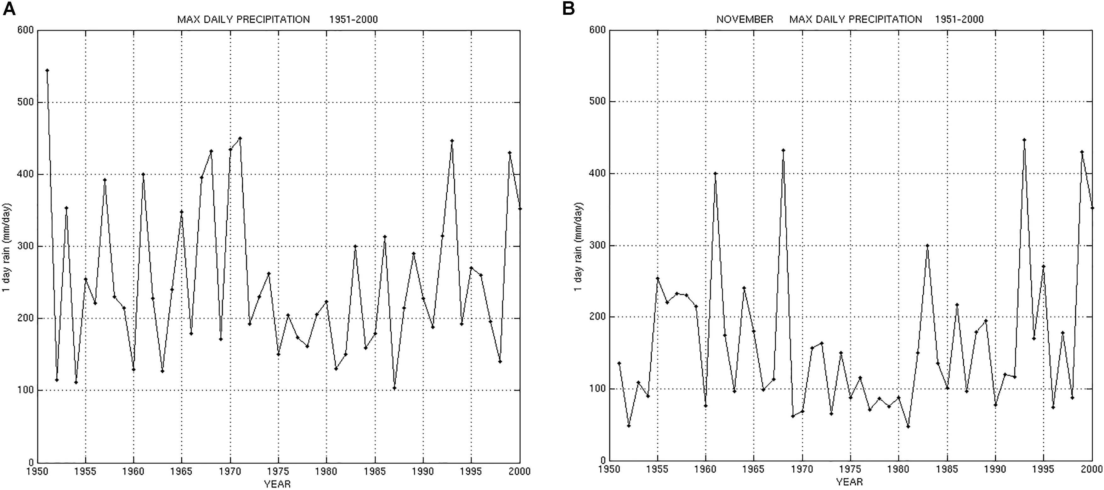
FIGURE 1. (A,B) Yearly series and November series (1951–2000).

FIGURE 2

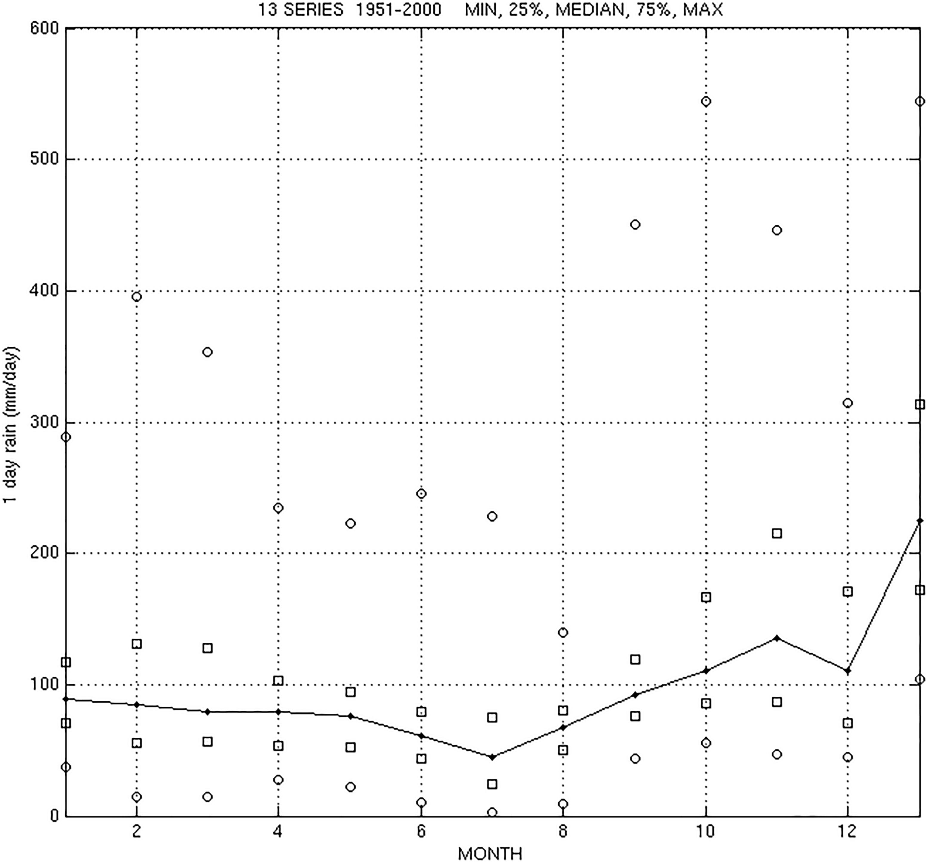
FIGURE 2. Minimum, 25%, median, 75%, maximum of 12 monthly and yearly series.

For simple mathematical reasons, the maximum value in a month or in a year should be higher (or equal) the denser the stations network is. In particular, we are interested to quantify the effects of the station density variation during 1951–2000. The dependence of this study results on network density is analyzed in Section “Dependence on Network Density. Sensitivity Study.”

Analysis of the Seasonal or Monthly Variation

In order to test the hypothesis that in October, November and December the extreme values are higher than in the other months of the year, as it appears in Figure 2, the Wilkoxon–Mann–Whitney rank sum test has been used (Wilks, 1995). It is a non-parametric test, so no hypothesis about the data distribution is assumed. Two monthly data at a time are compared; the aim is to test for a possible difference in location between them. The null hypothesis is that the two data batches have the same location. Table 1 presents the test results. It assumes a 5% threshold to reject the null hypothesis. Under this assumption the October and November series have the same location. In the Figure 2 the median, the 25% quantile and the 75% quantile in November look higher than the corresponding quantities in October, but this difference could be a statistical fluctuation (12%). The November values, on the contrary, are significantly higher than the December ones (4.8%). The December values are significantly higher than the January values (4.2%). In October values are significantly higher than in January (0.66%) and September (0.48%). November data are significantly higher than the other data except for October. The October data are significantly higher than the other data except for November and December. December data are significantly higher than the other data except for November and October. January, February, March and April do not present significant differences. The April series is significantly higher than the June one, while the June series is significantly higher than the July series. The August series is higher than the July one, but lower than the September series.

TABLE 1

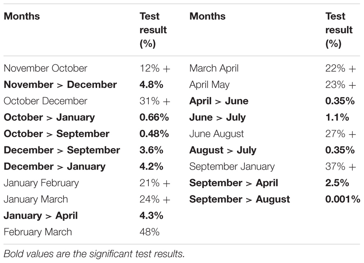
TABLE 1. Whitney rank sum test results for months comparison.

A possible explanation for the higher values in the autumn series, is that in October, November and to some extent in December, the convective precipitations are very intense in the Mediterranean region, due to the warm sea which provides a great amount of water vapor.

Analysis of Decadal Variation

The yearly series and the 12 monthly ones are analyzed in order to find significant variations between decades. Three kinds of analysis are performed. Two of them use the Wilkoxon–Mann–Whitney, the third analysis concerns the trend by using the Mann-Kendall test.

Comparison Between 1951–1975 and 1976–2000. Wilkoxon–Mann–Whitney Test With Decadal Mobile Window

The yearly series is separated into two parts: the data between 1951 and 1975, and the data between 1976 and 2000; then these two set of data are compared by using the Wilkoxon–Mann–Whitney test to find any differences in location between them. The same procedure is performed for each monthly series. The null hypothesis is that the two data batches have the same location. Table 2 presents the test results. It assumed a 5% threshold to reject the null hypothesis. Under this assumption the yearly series presents no significant differences between 1951–1975 data and 1976–2000 data (16%). The same results holds for the monthly series except for March. For most of them, the probabilities are much higher than the 5% threshold, only February and July show probabilities under 10%. In the case of March, the 1976–2000 data are significantly lower than the 1951–1975 data (2.3%).

TABLE 2

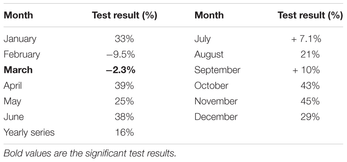
TABLE 2. Comparison between 1976–2000 and 1951–1975 by Wilkoxon–Mann–Whitney test.

The second kind of analysis by the Wilkoxon–Mann–Whitney test compares a decadal mobile window in the yearly series with the remaining data in the same series. The aim of this analysis is to find a decade where the data are significantly higher (or lower) than the remaining data in the series. The decade 1964–1973 (and 1965–1974) has significantly higher data than the other ones (with a 5% threshold). On the contrary the decades 1973–1982, 1975–1985, 1976–1985, and 1978–1987 have much lower data than the other ones.

Trends Assessed by Mann-Kendall Test

The Mann-Kendall test has been performed to find significant trend (if any) in the yearly and in each of the monthly series. The null hypothesis is that there is no trend. It assumed a 5% threshold to reject the null hypothesis. Table 3 presents the test results. The yearly series presents no significant trend (49%). This is consistent with the previous Wilkoxon–Mann–Whitney test results. All the monthly series, except for March and July, present no significant trend with probabilities higher than 10% (except for February, 8.7%). The March series shows a significant negative trend (>19 mm/day per decade), consistent with the Wilkoxon–Mann–Whitney test results. July data have a significant positive trend (8.5 mm/day per decade), while by using the Wilkoxon–Mann–Whitney test the result was not significant at 5% level (see Table 2). Figures 3A,B present the March and July series. The July trend is affected by the very high value of 228.4 mm/day in 1990 and perhaps by the 142.2 mm/day in 1999. Values greater than 200 mm/day are unusual in the Sardinia summer.

TABLE 3

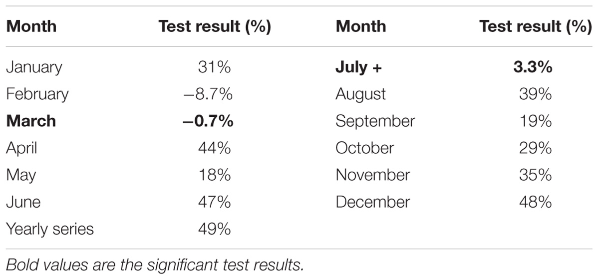
TABLE 3. Mann-Kendall trend test results.

FIGURE 3

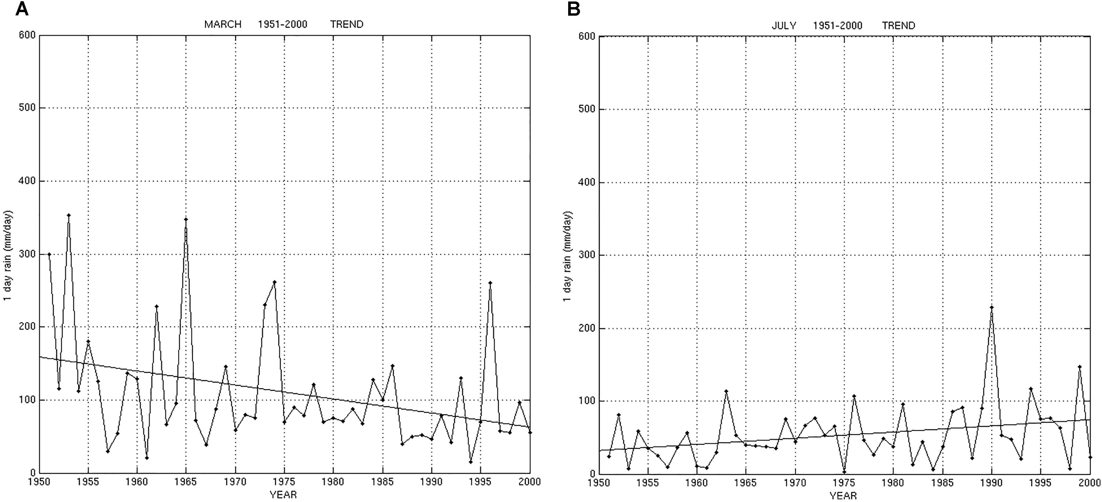
FIGURE 3. (A,B) March and July series and trend line.

Data Fitting by Theoretical Probability Distribution

The empirical Cumulative Distribution Function (CDF) is computed for the yearly series and for each monthly series as follows:

CDF = i/(50 + 1), i = 1,50

For each CDF, the corresponding empirical probability function is also derived. The Gumbel distribution is generally used in literature to fit extreme values distribution (Wilks, 1995). The probability Gumbel distribution is:

f(x) = 1/b^∗exp[−exp[(x−a)/b]−(x−a)/b].

The corresponding Cumulative Density Function is:

F(x) = exp[−exp[−(x−a)/b]].

The parameters a and b are calculated from the data.

b = s^∗sqrt(6)/3.1416… s is the data standard deviation.

a = m−0.57721^∗b m is the sample mean.

Therefore, 13 theoretical Gumbel distributions are obtained corresponding to the 13 empirical distribution of data. Each theoretical probability distribution is compared with the corresponding empirical one by Chi Square test. The null hypothesis is that the data were drawn from the fitted distribution, it is rejected at a 5% threshold level. Table 4 presents the Chi Square test results. The Gumbel probability function fits the yearly series (8.6%). The null hypothesis is rejected for September (0.1%) and October (1%) series. The January, March and May series are fitted with a test result between 5 and 10%. The remaining 7 series are fitted with a test result greater than 10%. The best fit results are February (40%), April (36.1%), and December (43.7%).

TABLE 4

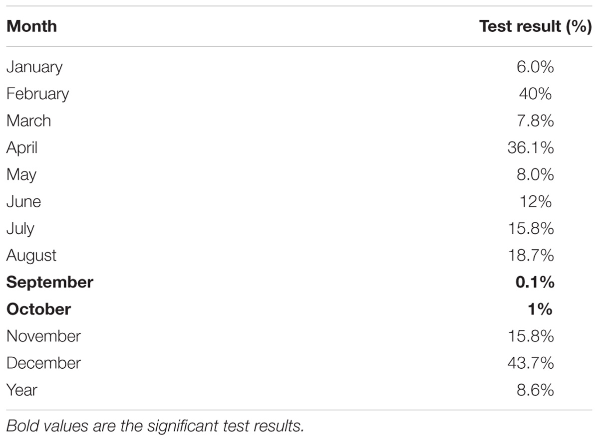
TABLE 4. Chi square test results for Gumbel fitting.

Figure 4 presents the empirical and the Gumbel CDF. In ordinate is (1-CDF) empirical and [1-F(x)] Gumbel, in abscissa is the yearly maximum of daily precipitation. Figures 5A–D present the (1-CDF) empirical and [1-F(x)] Gumbel for the January, April, July, and November representative series for each season.

FIGURE 4

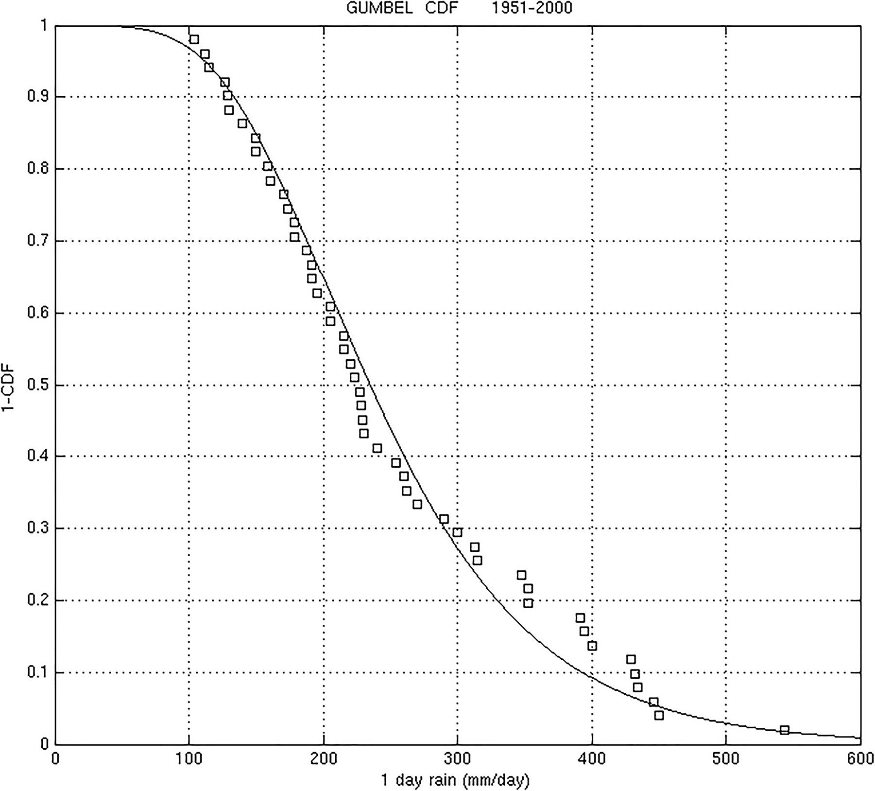
FIGURE 4. Empirical and Gumbel CDF for the yearly series.

FIGURE 5

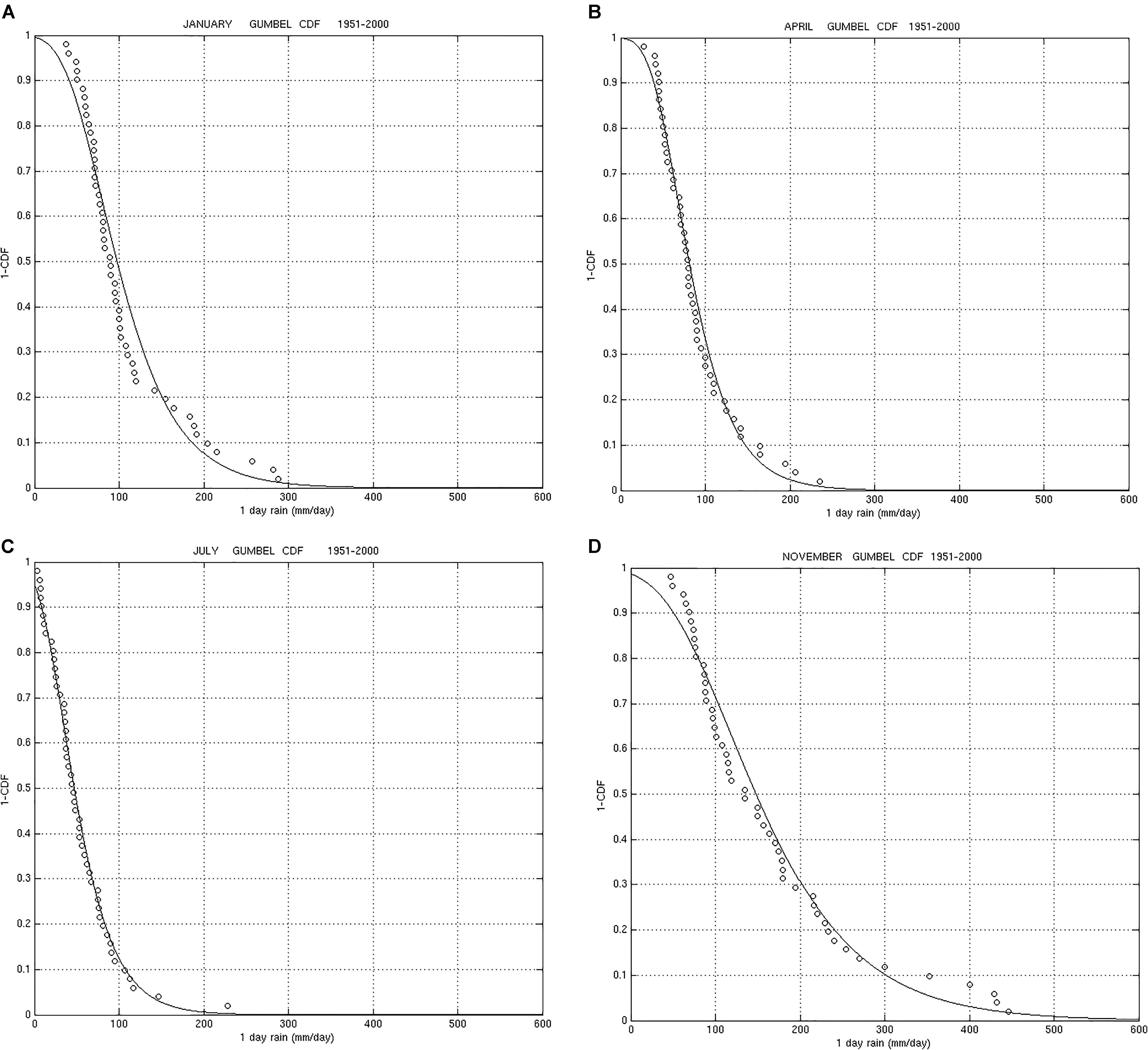
FIGURE 5. (A–D) Empirical and Gumbel CDF for January, April, July, and November.

The function [1-F(x)] Gumbel represents in ordinate the probability of a maximum daily cumulated precipitation greater than × over Sardinia in a year, in the case of yearly series, or in a month, in the case of monthly series. Then, from each Gumbel a probability table for different values of × can be made. Table 5 presents, for each month and for the year, the probability corresponding to different thresholds. The yearly probabilities range between 97% for 100 mm/day to 3% for 500 mm/day. Comparing the months, we can see that November produces the higher probabilities for all thresholds; they range between 71% for 100 mm/day to 0.9% for 500 mm/day. After November, October probabilities between 63% for 100 mm/day to 0.5% for 500 mm/day. December probabilities are very similar to October ones for low thresholds, such as 100 mm/day, but for higher thresholds they are very different: they range between 62% for 100 mm/day to 0.04% for 500 mm/day. March probabilities are similar to December ones. July and August present the lower probabilities for all the thresholds.

TABLE 5

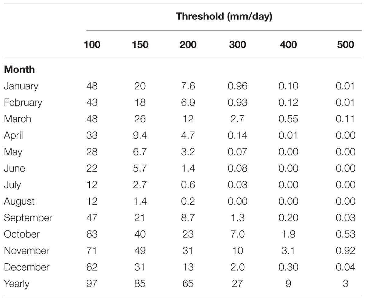
TABLE 5. Probabilities at different thresholds (mm/day).

Dependence on Network Density. Sensitivity Study

Figure 6A presents the stations location. Figure 6B shows the average number of stations for each year. It varies from 240 to 290, except for 1981 (212), 1982, 1983, 1984 (between 230 and 240), 1995 to 2000 (between 300 and 320). The mean distance between the stations varies from 10 Km (240 stations) to 9.1 Km (290 stations), except for the years 1981–1984 and 1995–2000. In this section we try to estimate the dependence of the previous results (monthly or seasonal variation, decadal variation, probability distributions, probabilities at different thresholds) on network density. A second set of stations is selected by excluding 60 stations (about 20% of the total) in a uniform spatial way; so, this set contains about 80% of the original one. A third set is selected, including only 60 stations, so it contains only 20% of the original set. Figure 7 shows the mean distance between the stations for the three data sets. We can see that the mean distance difference for the original and the second data set is very little, 1 or 2 Km. On the contrary, the mean distance for the third data set is about 20 Km. The analysis has been made on the annual series and on the January, March, July, September, October, and November series.

FIGURE 6

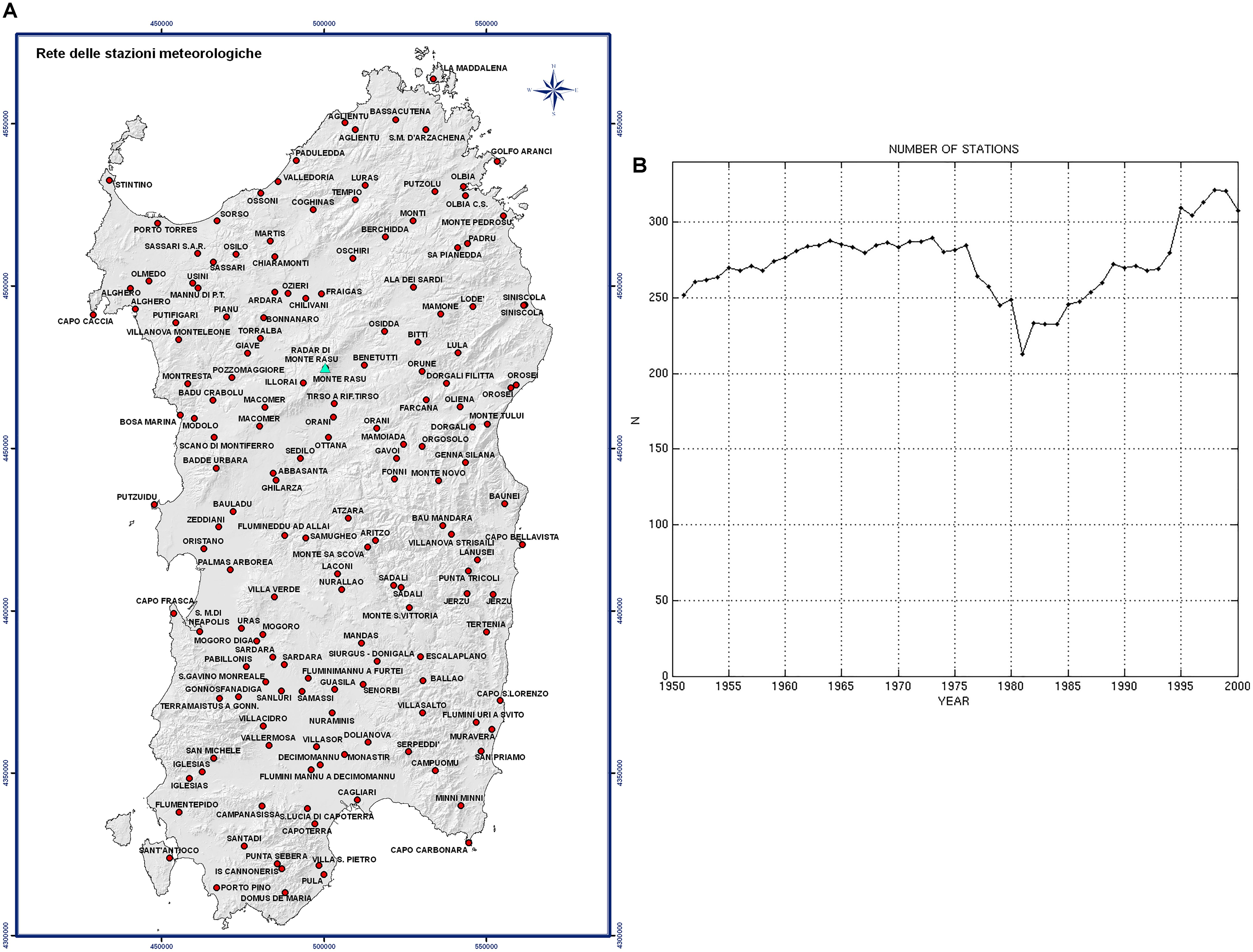
FIGURE 6. (A) Sardinia map with stations network. (B) Number of stations.

FIGURE 7

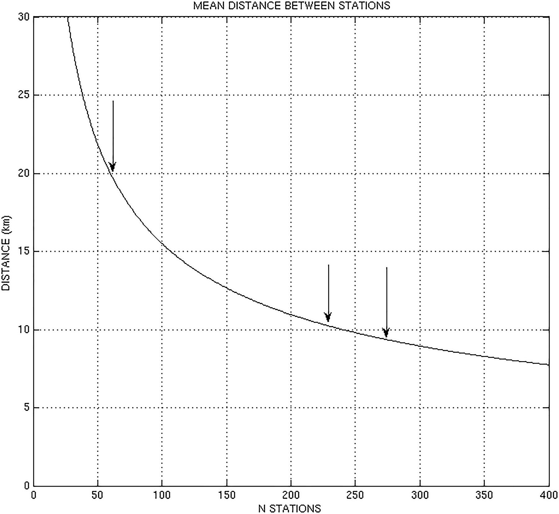
FIGURE 7. Mean distance between stations. The arrows correspond to the three dataset.

Exploratory Data Analysis

Figure 8 presents the 7 series of each data set summary; for the 6 monthly series (January, March, July, September, October, and November), and for the yearly one, the minimum, the 25% quantile, the median, the 75% quantile and the maximum are plotted. The continuous line plots the median. The original and the second data set very often have identical or almost identical medians. This is true for January, March, July, September, October and the annual series. The same is true for the other quantiles. On the contrary the third data set has much lower medians and the quantiles. For instance, in the yearly series, the original set median is 225.3 mm/day, the second set median is 217.9 mm/day, but the third set median drops to 180 mm/day. In the January series, the original set median is 89.4 mm/day, the second set median is 86 mm/day, but the third set median is 56.9 mm/day. In the July series, the original set median is 45 mm/day, the second set median is again 45 mm/day, but the third set median is 21.6 mm/day.

FIGURE 8

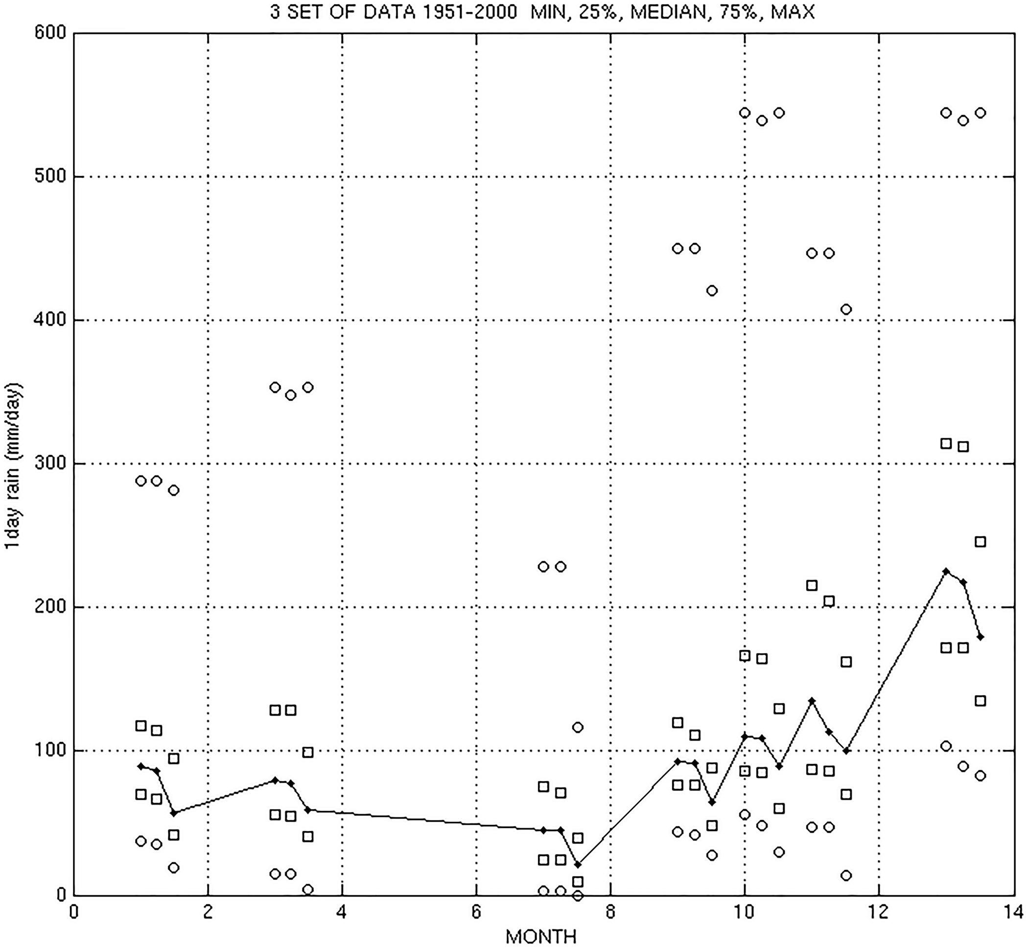
FIGURE 8. Summary of three data set. Minimum, 25%, median, 75%, maximum for January, March, July, September, October, November, and yearly series.

Data Fitting by Theoretical Probability Distribution

Figure 9 presents (1−CDF) empirical and [1−F(x)] Gumbel for yearly data. It is evident that the original and the second data set are very similar. The third data set has a very different empirical and theoretical distribution. Even for monthly series, the original and the second data set have very similar distributions, while the third data set distributions are very different. In Figure 9, yearly series, the probability of events greater than 150 mm/day is 85% for the original dataset, 83% for the second data set, but it decreases to 69% for the third data set. The probability of events greater than 200 mm/day is 65% for the original dataset, 62% for the second data set, but only 44% for the third data set. For the November distributions: the probability for events greater than 150 mm/day is 49% for the original dataset, 46% for the second data set, but it decreases to 32% for the third data set; the probability of events greater than 200 mm/day is 31% for the original dataset, 29% for the second data set, but only 15% for the third data set. Similar results hold for the other months.

FIGURE 9

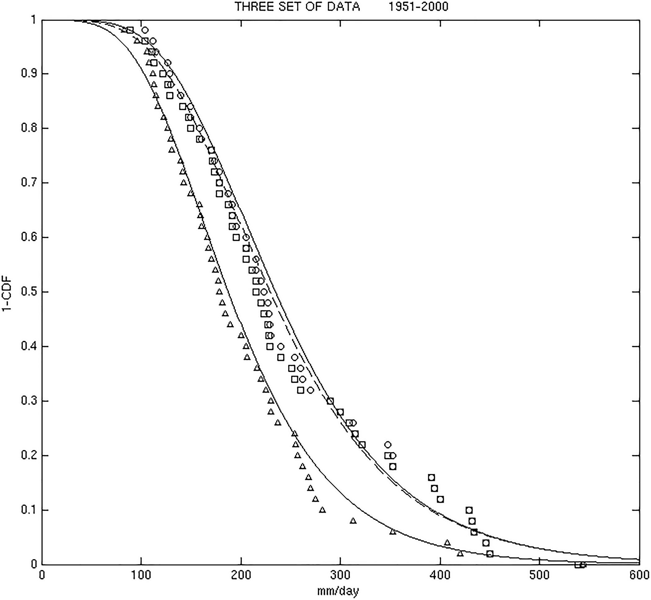
FIGURE 9. Three set of data; original one (circle), second set (squares), third set (triangles). Yearly series. The continuous lines represent the fitting Gumbel.

Three Data Set Comparison by Wilkoxon–Mann–Whitney Test

The second and the third data set have been compared to the original one by using the rank sum test (Wilkoxon–Mann–Whitney) to find any differences in location between them. This has been made again for the yearly series and for the January, March, July, September, October, and November series. The null hypothesis is that the two data batches have the same location. Table 6 presents the test results: in the second column the comparison between the original and the second data set is shown, in the third column, the comparison between the original and the third one. Again, a 5% threshold has been assumed to reject the null hypothesis. The second data set and the original one have the same location, with a test result much higher than 5%: the yearly series shows 37% and the monthly series between 29% (November) and 44% (July). On the contrary, the third data set is completely different from the original one. All the test results are below 1% except for November (2%). In particular, the yearly series has a test result of 0.26%.

TABLE 6

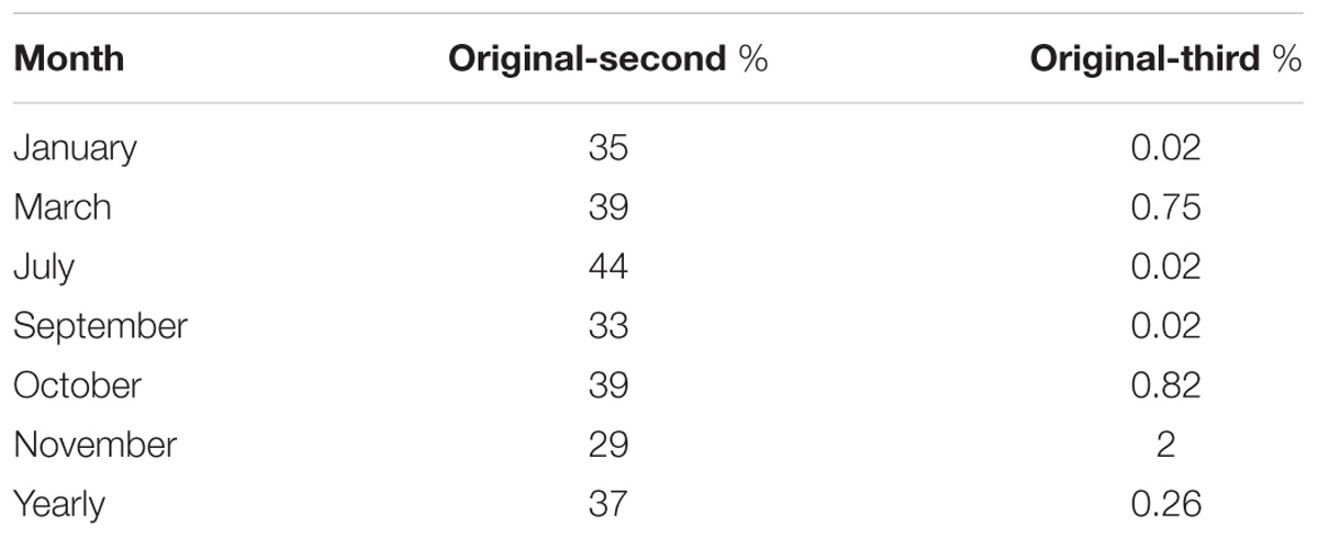
TABLE 6. Comparison between three data set: Wilkoxon–Mann–Whitney (sum rank) test results.

The meaning of this test is as follows: in the second data set the station to station mean distance is not much lower than the original one, so the network can catch almost all the rain events as the original network. On the contrary, in the third data set the station to station mean distance is much higher than in the original network (20 Km vs. 10 Km), so that many rain events have not been detected.

Comparison Between 1951–1975 and 1976–2000 by the Wilkoxon–Mann–Whitney Test

The test as of Section “Comparison Between 1951–1975 and 1976–2000. Wilkoxon–Mann–Whitney Test With Decadal Mobile Window” (Wilkoxon–Mann–Whitney) has been repeated by using the third data set (low density network), which is very different in location from the original one. Again the yearly series is separated into two equal parts: the data between 1951 and 1975, and the data between 1976 and 2000. The same procedure is performed for each of the monthly series. These two set of data are compared by the Wilkoxon–Mann–Whitney test to find any differences in location between them. The null hypothesis is that the two data batches have the same location. Table 7 presents the test results. It assumed a 5% threshold to reject the null hypothesis. The test result for the yearly series is 3.6%, so the 1951–1975 series is significantly higher than 1976–2000 series. On the contrary, the test result of Section “Comparison Between 1951–1975 and 1976–2000. Wilkoxon–Mann–Whitney Test With Decadal Mobile Window,” obtained by using the original data set, was 16%. The test results for monthly series are similar to those obtained by the original data set shown in Section “Comparison Between 1951–1975 and 1976–2000. Wilkoxon–Mann–Whitney Test With Decadal Mobile Window.” In particular, for March, the significant decreasing in location from 1951–1975 to 1976–2000 is confirmed (1.1%). However, it must be remarked that for September the test result changes from 10% with the original data set to 27%, and for July it changes from 7.1 to 16%.

TABLE 7

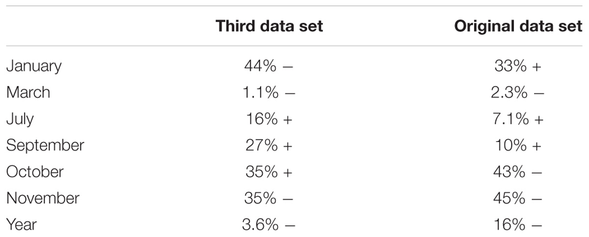
TABLE 7. Dependence on network density. Comparing 1951–1975 and 1976–2000 by Wilkoxon–Mann–Whitney test results.

Trends by Mann-Kendall Test

The Mann-Kendall trend test has been repeated by using the second and the third data set. As in Section “Trends Assessed by Mann-Kendall Test,” the null hypothesis is that there is no trend; a 5% threshold is assumed to reject the null hypothesis. Table 8 presents the test results. The second data set and the original one produce very similar results, as expected. The third data set for the July series produces a trend that is not significant, contrary to the other two data set. Also the yearly series results for the third data set (7.3%) is completely different from the original data set (49%) and from the second one (38%).

TABLE 8

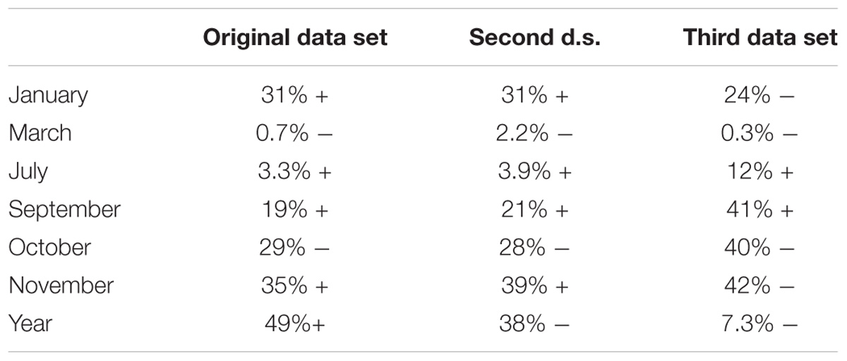
TABLE 8. Dependence on network density. Mann-Kendall trend test results.

Special Test: Year 1981 (Lower Network Size)

In 1981 the number of stations dropped to 212. In the yearly series the 1981 value is 130 mm/day. We can suspect that this value could be affected by the low number of stations and as a consequence it affects some of the previous results. To test this hypothesis, a much higher value is inserted in the yearly series corresponding to 1981: 223 mm/day (which it is the annual series median) instead of 130 mm/day. Then the Wilkoxon–Mann–Whitney test as of Section “Comparison Between 1951–1975 and 1976–2000. Wilkoxon–Mann–Whitney Test With Decadal Mobile Window” has been repeated, to compare a decadal mobile window in the yearly series with the remaining data in the same series. The results are very similar to the ones shown in Section “Comparison Between 1951–1975 and 1976–2000. Wilkoxon–Mann–Whitney Test With Decadal Mobile Window.” The decade 1964–1973 (and 1965–1974) have significantly higher data than the other ones (with a 5% threshold); on the contrary the decades 1975–1985 and 1976–1985 have significantly lower data than the other ones. The Mann-Kendall test for the trend (see Trends Assessed by Mann-Kendall Test) has been repeated too. The new test result is 47%, not much different from the previous one (49%). It confirms the absence of any trend. The Mann-Kendall test for the trend has also been repeated by using 300 mm/day instead of 130 mm/day; the new test result is again similar to what is presented in Section “Trends Assessed by Mann-Kendall Test”: 46%.

Special Test Over 1995–2000 (Higher Network Size)

During 1995–2000, about 60 new stations were added. In order to test the effect of this change on the trend test, the annual precipitation maxima series has been reconstructed after excluding the 60 new stations. This exclusion changes the station to station mean distance very little. The result is that the new series is the same as the previous one, so the trend test is not influenced by the higher network size in 1995–2000. This result is consistent with the three set tests as of Sections “Three Data Set Comparison by Wilkoxon–Mann–Whitney Test,” “Comparison Between 1951–1975 and 1976–2000 by the Wilkoxon–Mann–Whitney Test,” “Trends by Mann-Kendall Test.”

Conclusion

Fifty years (1951–2000) of daily precipitations data for Sardinia have been analyzed in order to study the extreme events on monthly or annual base. Twelve monthly and 1 yearly series sized 50 of daily precipitation maxima have been analyzed. The comparisons among the monthly series by using the Wilkoxon–Mann–Whitney test show that October, November, and December series have significantly higher values than all the other months. A possible explanation is that in autumn the Mediterranean sea temperature is high, so that great quantities of water vapor are available and support atmospheric instability and convective precipitations. Sea surface temperature is high in summer, too, but the cyclone activity is very low, due to the northern displacements of trajectories; as a consequence, summer is a dry season in Sardinia and in most of Mediterranean areas.

Comparison of decades has been made by using the Wilkoxon–Mann–Whitney test. The series, except the March one, present no significant difference between the 1951–1975 and 1976–2000 periods. In the case of March series the 1976–2000 data are significantly lower than the 1951–1976 data, with a test result of 2.3%. The Wilkoxon–Mann–Whitney test is used again to compare a decadal mobile window to the remaining data in the yearly series. The decade 1964–1973 (and 1965–1974) has significantly higher data than the other ones (with a 5% threshold). On the contrary the decades 1973–1982, 1975–1985, 1976–1985, and 1978–1987 have significantly lower data than the other ones.

The 13 series are also analyzed by the Mann-Kendall trend test. The yearly series presents no trend (49%). Even the monthly series, except for the July and March ones, have no trend. The March series has a significant negative trend (−19 mm/day per decade), while July shows a significant positive trend (8 mm/day per decade).

The 13 data sets are fitted by the Gumbel probability function. The Chi Square test is used to evaluate the fit. The test result for the yearly series is 8.6%. Seven monthly series have a test result between 10 and 43.7%, 3 monthly series between 5 and 10%. September and October data are not fitted adequately by the Gumbel function, the test result is lower than 5% (0.1 and 1%). A further analysis is necessary to understand the peculiarity of September and October data.

In order to quantify the dependence of the previous results on the network density, two other dataset are defined. One of them is obtained by excluding 60 stations (about 20% of the total) in a uniform spatial way. The other data set is obtained by excluding about 80% of the stations, so that it includes only 60 stations. So, the station to station mean distance varies from nearly 9 Km for the original dataset, to nearly 11 Km for the second one, to nearly 20 Km for the third dataset. The previous analysis have also been performed for the other two dataset. The second and the third dataset have been compared to the original one by the Wilkoxon–Mann–Whitney test. The second dataset presents no significant difference, with test results much higher than 30%; on the contrary, the third dataset values are significantly lower than the original ones. The Gumbel function fitted from the third data set has much lower probability values than the other two; for instance, the probability for events greater than 200 mm/day in a year is 65% for the original dataset, 62% for the second data set, but only 44% for the third data set. Also, the comparison among decades, with the third data set, gives different results than the original one; for instance, the 1951–1975 period shows significantly higher values than the 1976–2000 (3.6%), while according to the original data set there is no significant difference (16%).

In this analysis, Sardinia has been considered as homogeneous as regard rainfall climatology. Actually, that is not completely true, because the Gennargentu mountain divides Sardinia into an east side and a west side area with different rainfall climatology (Benzi et al., 1997). As pointed out in Boi and Marrocu (2011), the cyclones associated with very intense rainfall events mostly strikes the east side area. So, a future analysis should consider dividing Sardinia in two separate climatic zones. Another point that could be investigated is a different duration interval, not only 1-day, but also 2-days or 5-days precipitation extremes. Also, a seasonal analysis, instead of the monthly one, could be better. At the same time, a more general distribution, like GEV, could be used instead of the Gumbel distribution. Another object of investigation could be a different variable: annual maxima of normalized rainfall instead of annual maxima of rainfall.

Author Contributions

The author confirms being the sole contributor of this work and has approved it for publication.

Conflict of Interest Statement

The author declares that the research was conducted in the absence of any commercial or financial relationships that could be construed as a potential conflict of interest.

Acknowledgments

I’m grateful to Francesco Battaglia for his kind help in the final revision. I thank two reviewers for their critical comments on this paper.

References

Benzi, R., Deidda, R., and Marrocu, M. (1997). Characterization of temperature and precipitation fields over Sardinia with principal component analysis and singular spectrum analysis. Int. J. Climatol. 17, 1231–1262. doi: 10.1002/(SICI)1097-0088(199709)17:11<1231::AID-JOC170>3.0.CO;2-A

CrossRef Full Text | Google Scholar

Bodini, A., and Cossu, Q. A. (2008). Analisi. (Della) Piovosità in Ogliastra nel Periodo 1951-1999. Rapporto interno. 2008-IMATI MI/4. Lombardia: Istituto di Matematica Applicata e Tecnologie Informatiche CNR.

Google Scholar

Boi, P., and Marrocu, M. (2011). Frequency, seasonal dependence and synoptic scale patterns of cyclones associated to very intense rainfall on Sardinia island. Geophys. Res. Abstract 13:EGU2011-1491-1.

Google Scholar

Brienen, S., Rapala, A., Machel, H., and Simmer, C. (2013). Regional centennial precipitation variability over Germany from extended observation records. Int. J. Climatol. 33, 2167–2184. doi: 10.1002/joc.3581

CrossRef Full Text | Google Scholar

Brugnara, Y., Brunetti, M., Maugeri, M., Nanni, T., and Simolo, C. (2011). High-resolution analysis of daily precipitation trends in the central Alps over the last century. Int. J. Climatol. 32, 1406–1422. doi: 10.1002/joc.2363

CrossRef Full Text | Google Scholar

Brunetti, M., Colacino, T., Maugeri, M., and Nanni, M. (2001a). Trends in the daily intensity of precipitation in Italy from 1951 to 1996. Int. J. Climatol. 21, 299–316. doi: 10.1002/joc.613

CrossRef Full Text | Google Scholar

Brunetti, M., Maugeri, M., and Nanni, M. (2001b). Changes in total precipitation, rainy days and extreme events in northeastern Italy. Int. J. Climatol. 21, 861–871. doi: 10.1002/joc.660

CrossRef Full Text | Google Scholar

Brunetti, M., Maugeri, M., Monti, F., and Nanni, M. (2006). Temperatures and precipitation variability in Italy in the last two centuries from homogenised instrumental time series. Int. J. Climatol. 26, 345–381. doi: 10.1002/joc.1251

CrossRef Full Text | Google Scholar

Fowler, H. J., and Kilsby, C. G. (2003). A regional frequency analysis of United Kingdom extreme rainfall from 1961 to 2000. Int. J. Climatol. 23, 1313–1334. doi: 10.1002/joc.943

CrossRef Full Text | Google Scholar

Jones, M. R., Fowler, H. J., Kilsby, C. G., and Blenkinsop, S. (2013). An assessement of changes in seasonal and annual extreme rainfall in the UK between 1961 and 2009. Int. J. Climatol. 33, 1178–1194. doi: 10.1002/joc.3503

CrossRef Full Text | Google Scholar

Moberg, A., and Jones, P. D. (2005). Trends in indices for extremes in daily temperatures and precipitation in central and western Europe, 1901-99. Int. J. Climatol. 25, 1149–1171. doi: 10.1002/joc.1163

CrossRef Full Text | Google Scholar

Pavan, V., Tomozeiu, R., Cacciamani, C., and Di Lorenzo, M. (2008). Daily precipitation observations over Emilia-Romagna: mean values and extremes. Int. J. Climat. 28, 2065–2079. doi: 10.1002/joc.1694

CrossRef Full Text | Google Scholar

Piccarreta, M., Pasini, A., Capolongo, A., and Lazzari, M. (2013). Changes in daily precipitation extremes in the Mediterranean from 1951 to 2010: the Basilicata region, southern Italy. Int. J. Climatol. 33, 3229–3248. doi: 10.1002/joc.3670

CrossRef Full Text | Google Scholar

Rodrigo, F. S., and Trigo, R. M. (2007). Trends in daily rainfall in the Iberian Peninsula from 1951 to 2002. Int. J. Climatol. 27, 513–529. doi: 10.1002/joc.1409

CrossRef Full Text | Google Scholar

Santos, M., and Fragoso, M. (2012). Seasonal trends in extreme daily precipitation indices in Nothern of Portugal. Geophys. Res. Abstracts 14:EGU2012-8292.

Google Scholar

Schmidli, J., and Frei, C. (2005). Trends of heavy precipitation and wet and dry spells in Switzerland during the 20th century. Int. J. Climatol. 25, 753–771. doi: 10.1002/joc.1179

CrossRef Full Text | Google Scholar

Tank, A. M. G. K., and Konnen, G. P. (2003). Trends in indices of daily temperature and precipitation extremes in Europe, 1946-99. J. Clim. 16, 3665–3680. doi: 10.1175/1520-0442(2003)016<3665:TIIODT>2.0.CO;2

CrossRef Full Text | Google Scholar

Wilks, D. S. (1995). Statistical Methods in the Atmospheric Sciences. San Diego, CA: Academic Press Inc.

Google Scholar