Abstract
Open-access global Digital Elevation Models (DEM) have been crucial in enabling flood studies in data-sparse areas. Poor resolution (>30 m), significant vertical errors and the fact that these DEMs are over a decade old continue to hamper our ability to accurately estimate flood hazard. The limited availability of high-accuracy DEMs dictate that dated open-access global DEMs are still used extensively in flood models, particularly in data-sparse areas. Nevertheless, high-accuracy DEMs have been found to give better flood estimations, and thus can be considered a ‘must-have’ for any flood model. A high-accuracy open-access global DEM is not imminent, meaning that editing or stochastic simulation of existing DEM data will remain the primary means of improving flood simulation. This article provides an overview of errors in some of the most widely used DEM data sets, along with the current advances in reducing them via the creation of new DEMs, editing DEMs and stochastic simulation of DEMs. We focus on a geostatistical approach to stochastically simulate floodplain DEMs from several open-access global DEMs based on the spatial error structure. This DEM simulation approach enables an ensemble of plausible DEMs to be created, thus avoiding the spurious precision of using a single DEM and enabling the generation of probabilistic flood maps. Despite this encouraging step, an imprecise and outdated global DEM is still being used to simulate elevation. To fundamentally improve flood estimations, particularly in rapidly changing developing regions, a high-accuracy open-access global DEM is urgently needed, which in turn can be used in DEM simulation.
Introduction
Digital Elevation Models (DEM) are a gridded digital representation of terrain, with each pixel value corresponding to a height above a datum. Since the pioneering work of Miller and Laflamme (1958), DEMs have grown to become an integral part of a number of scientific applications. DEMs can be created from ground surveys, digitizing existing hardcopy topographic maps or by remote sensing techniques. DEM’s are now predominantly created using remote sensing techniques with Smith and Clark (2005) observing the benefits that a large spatial area can be mapped by fewer people at a lower cost. Remotely sensing techniques include photogrammetry (Uysal et al., 2015; Coveney and Roberts, 2017), airborne and spaceborne Interferometric Synthetic Aperture Radar (InSAR) and Light Detection And Ranging (LiDAR). Spaceborne InSAR is the most common technique to create global DEMs and is the technology behind the most widely used open-access global DEM; the Shuttle Radar Topography Mission (SRTM). An overview of free and commercial global DEMs is given in Figure 1. Despite being acquired in 2000, SRTM is still the most popular global DEM because of its accessibility, feature resolution, vertical accuracy and a lower amount of artifacts and noise compared to alternative global DEMs (Rexer and Hirt, 2014; Jarihani et al., 2015; Sampson et al., 2016; Hu et al., 2017). Yet, recently released products such as MERIT and TanDEM-X 90 could change that. Commercial DEMs (Planet Observer, 2017; Takaku and Tadono, 2017; InterMap, 2018) are often prohibitively costly and have a lack of comparison studies. Airborne LiDAR has a higher precision and accuracy owing to its ability to penetrate vegetation and its reduced vulnerability to scatter but is largely limited to a handful of countries and can be expensive to acquire. These characteristics are conducive in creating a high-quality (vertical error <1 m) ‘bare-earth DEM,’ where objects (e.g., buildings and vegetation) have been removed from the elevation model. Such bare-earth DEMs are essential for applications, such as flood modeling, that rely on the accurate derivation of surface characteristics (e.g., slope).
FIGURE 1
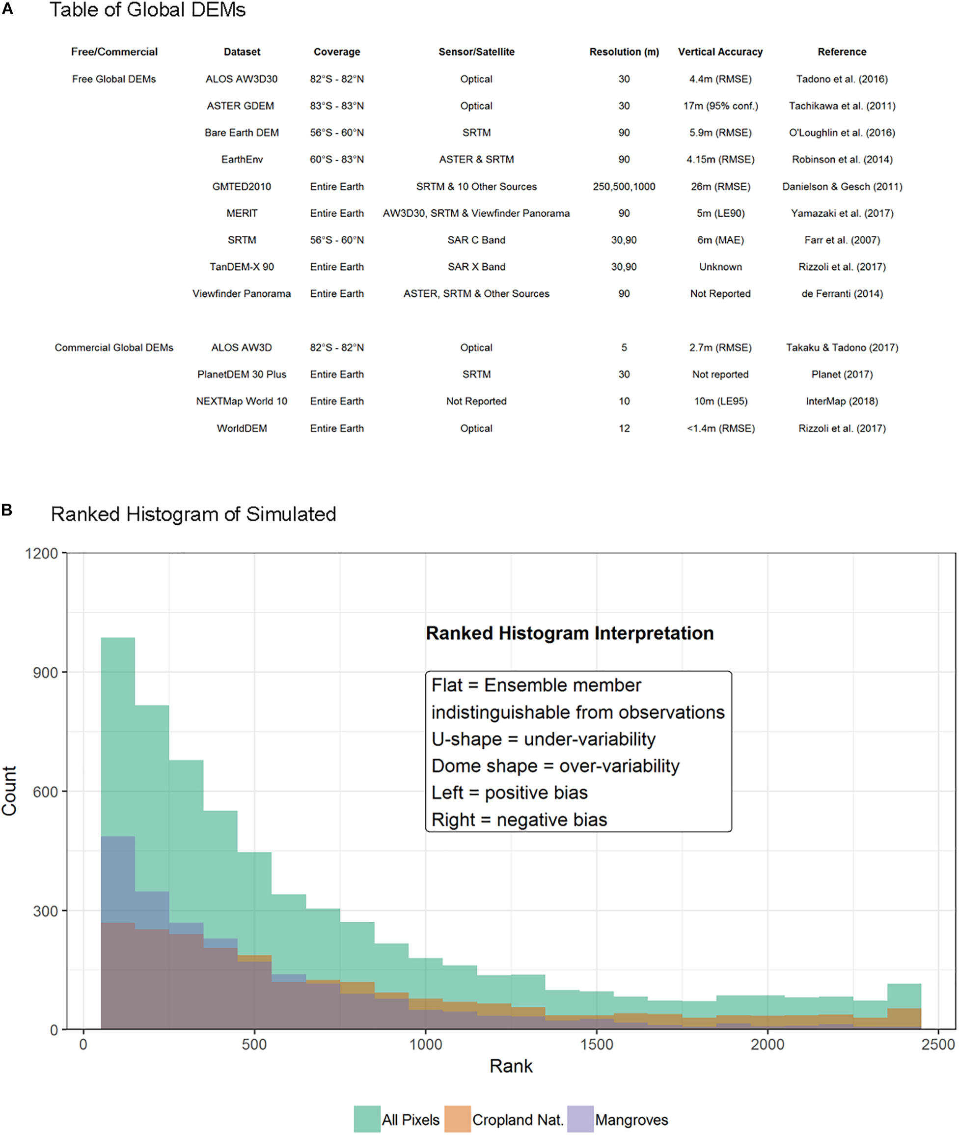
(A) Overview of Existing Global DEMs (free and commercial). (B) Rank Histograms for an ensemble of 2500 DEMs of the Ba catchment in Fiji, simulated from the MERIT DEM using semi-variograms of spatial error structure by landcover class. All Pixels and the two landcover classes with the most pixels (Mosaic Cropland/Natural Vegetation and Mangroves) are shown.
Characteristics of DEM Errors
DEM errors occur in both the horizontal and vertical directions. Errors propagate from the input data used in creating a DEM right through to calculating surface derivatives and using DEMs in complex applications (Hutchinson and Gallant, 2000; Fisher and Tate, 2006). Whatever their source, DEMs can appear to provide a definitive and plausible representation of topography which can often lull the user into a false sense of security regarding their accuracy, with many users unaware of DEM errors or how to treat them (Wechsler, 2003, 2007). Whilst accuracy statistics such as RMSE provide an indication of DEM accuracy, they assume error to aspatial (Hunter and Goodchild, 1997; Carlisle, 2005; Fisher and Tate, 2006; Wechsler, 2007). Invoking Tobler’s First Law of Geography, whereby he noted that “nearby things are more similar than distant things” (Tobler, 1970), we know error varies spatially so DEM error is spatially autocorrelated. Indeed, Holmes et al. (2000) observe that “although global (average) error is small, local error values can be large, and also spatially correlated.” The spatial variation of DEM error is most frequently estimated by calculating accuracy statistics of areas disaggregated by slope and/or landcover class, and more rarely spatial structure of error.
Wise (2000) categorized DEM errors as systematic, blunders or random. These types of errors derive from: (a) deficient spatial sampling and/or age of data; (b) processing errors such as interpolation or numerical errors; (c) measurement errors from poor positional inaccuracy, faulty equipment or observer bias (Wechsler, 2007). Systematic errors occur in the DEM creation procedure by processing techniques that can cause bias or artifacts. Blunders arise from human error (Wise, 2000) or equipment failure (Fisher and Tate, 2006). Random errors occur in any system of measurement due to the wealth of measurement and operational tasks performed to create a DEM (Wise, 2000; Fisher and Tate, 2006), and remain even after known blunders and systematic errors are removed (Wechsler, 2007). An example of random error is speckle noise (multiplicative noise in a granular pattern) (Rodriguez et al., 2006; Farr et al., 2007). Sources of systematic errors and blunders relevant to flood modeling derive from interpolation techniques (Desmet, 1997; Wise, 2007; Bater and Coops, 2009; Guo et al., 2010), erroneous sink filling (Burrough and McDonnell, 1998), hydrological correction (Callow et al., 2007; Woodrow et al., 2016), deficient spatial sampling causing urban features not to be resolved (Gamba et al., 2002; Farr et al., 2007), slope and aspect (foreslope vs backslope) (Toutin, 2002; Falorni et al., 2005; Shortridge and Messina, 2011; Szabó et al., 2015), striping caused by instrument setup (Walker et al., 2007; Tarakegn and Sayama, 2013) and vegetation (Carabajal and Harding, 2006; Hofton et al., 2006; Shortridge, 2006; Weydahl et al., 2007; LaLonde et al., 2010).
The aforementioned errors propagate into errors in surface derivatives including, but not limited to, slope (Holmes et al., 2000), aspect (Januchowski et al., 2010), curvature (Wise, 2011), drainage basin delineation (Oksanen and Sarjakoski, 2005) and upslope contributing area (Wu et al., 2008). As many models rely on these surface derivatives (e.g., change in slope is the dominant control on flow in flood models), error propagation from DEMs can substantially affect results of models that use these surface derivatives. Yet, taking flood models as an example, sensitivity analysis has largely focussed on hydraulic parameters and has under-represented DEM errors (Wechsler, 2007). Davis and Keller (1997) aptly sum up the problem of DEM error with their remark that ‘landscapes are not uncertain, but knowledge about them is.’
Flood Inundation Models and DEM Error
Topography is arguably the key factor for the estimation of flood extent (Horritt and Bates, 2002), but typically flood models use a limited number of DEMs and instead choose to explore the uncertainty associated with other hydraulic parameters (Wechsler, 2007). Studies that do use multiple DEMs either resample DEMs to a coarser resolution to explore the effect of resampling strategies and/or scale (Horritt and Bates, 2001; Neal et al., 2009; Fewtrell et al., 2011; Saksena and Merwade, 2015; Savage et al., 2016b; Komi et al., 2017), or compare flood extents using different DEM products (Li and Wong, 2010; Jarihani et al., 2015; Bhuyian and Kalyanapu, 2018). Generally speaking, the quality of flood predictions increases with higher resolution DEMs. Higher resolution DEMs are more important when modeling urban environments (Fewtrell et al., 2008) so buildings can be captured. Resolution can be less important for rural environments with Savage et al. (2016a) concluding that running simulations finer than 50 m had little performance gain without occurring additional unnecessary computational cost. Too much detail can induce spuriously precise results which does not represent the uncertainties in making flood predictions (Dottori et al., 2013; Savage et al., 2016a). In data-sparse regions, a limited number of global DEM products dictates that only a single DEM is used, with this most commonly being SRTM (Yan et al., 2015). Whilst understandable, using a single DEM leads to a dangerous situation where spuriously precise estimates of flood extent are presented which do not assess the impact of uncertain topography. DEM simulation overcomes this obstacle by making available a catalog of statistically plausible DEMs at the native resolution of the global DEM from which it is simulated from.
Current Advances – Correcting DEM Error
Here we identify three categories of approaches to correct DEM error: (1) DEM editing; (2) New DEMs created with improved sensing technologies and (3) Stochastic simulation of DEMs. This article focuses on the third approach.
DEM Editing
DEM error can be reduced by editing – either manually or systematically. Manual editing involves changing pixel values based on additional information or expert judgement. We speculate that this happens frequently but is seldom documented. Systematic editing involves applying algorithms, additional datasets and filters to reduce error. For example, a DEM can be hydrologically corrected through algorithms such as AGREE (Hellweger, 1997), ANUDEM (Hutchinson, 1989), outlet breaching (Martz and Garbrecht, 1999), Priority-Flood (Barnes et al., 2014) and stream burning (Saunders, 1999). Namely, the HydroSHEDs global hydrography dataset makes use of hydrological correction techniques to create invaluable maps such as flow direction, river networks and catchment masks (Lehner et al., 2008). DEMs have also been edited to correct errors from vegetation (Baugh et al., 2013; Pinel et al., 2015; Su et al., 2015; O’Loughlin et al., 2016; Ettritch et al., 2018; Zhao et al., 2018) and to compensate for the positive bias in coastal areas due to vegetation and buildings that lead to an underestimation of coastal flood exposure [e.g., CoastalDEM (Kulp and Strauss, 2018)].
The recent release of the MERIT (Multi-Error-Removed-Improved-Terrain) DEM is the most comprehensive error removal from SRTM to date. Errors are reduced by separating and removing absolute bias, stripe noise, speckle noise and vegetation bias, with the most significant improvements reported in flat regions (Yamazaki et al., 2017). Compared to SRTM, MERIT has fewer artifacts (Hirt, 2018) and a better performance in flood models compared to SRTM (Chen et al., 2018). Whilst a significant improvement on SRTM, MERIT is still fundamentally based on SRTM data and is thus limited by the errors in SRTM. The next new edited DEM will be NASADEM (Crippen et al., 2016) set to be released in 2018, but again this is a reprocessing of SRTM.
New DEMs
The most widely used open-access global DEM (SRTM) is almost two decades old. Advances in satellite technology, image processing and data storage capabilities, make creating new, more accurate DEMs entirely possible. Two new global DEMs have been recently released, namely optically derived ALOS AW3D30 (Tadono et al., 2014) (∼30 m resolution) and the SAR derived TanDEM-X 90 (Rizzoli et al., 2017) (∼90 m resolution). Both of these products are technically digital surface models, so should only be used with caution in flood models. Looking to the future, new techniques are being explored to create new DEMs. One such example of applying a new technique is the creation of a 2 m pan-Arctic DEM (ArcticDEM)1 using stereo auto-correlation techniques to overlap pairs of high-resolution optical imagery. Additionally, Ghuffar (2018) demonstrated that a 5 m DEM can be generated from Planet Labs cubesat derived PlanetScope imagery using Semi Global Matching. Alternatively, existing DEMs can be fused together to create new products (de Ferranti, 2014; Yue et al., 2017; Pham et al., 2018). For example ASTER and SRTM have been fused together to create the global EarthEnv DEM (Robinson et al., 2014). High Resolution (<10 m) open-access LiDAR data is becoming increasingly available through initiatives such as OpenTopography2, with New Zealand the latest country to release LiDAR data for free. Despite this encouraging step, we optimistically estimate open-access LiDAR data covers just 0.005% of the earth′s land area based on data from OpenTopography and an extensive search of national mapping agencies. Global LiDAR coverage is some way off, with the limited amount of LiDAR data that is currently available almost exclusively found in developed countries.
DEM Simulation
Stochastic simulation assumes that a DEM is only a single realization amongst a host of potential realizations. DEMs are simulated by altering pixel values in accordance with the spatial error structure. A single true DEM is not created. Instead realizations provide a bound within which the true value is likely to lie. Therefore, DEM error is not reduced as such, but the bounds of error are identified. This idea is relatively well known in the field of geostatistics (Goovaerts, 1997; Hunter and Goodchild, 1997; Deutsch and Journel, 1998; Kydriakidis et al., 1999; Holmes et al., 2000). Using an ensemble of simulated DEMs has been shown to greatly affect the characterization of surface derivatives (Fisher, 1991; Veregin, 1997; Holmes et al., 2000; Endreny and Wood, 2001; Raaflaub and Collins, 2006), landslide hazard (Davis and Keller, 1997; Murillo and Hunter, 1997; Darnell et al., 2008) and flood inundation estimation (Wilson and Atkinson, 2005; Hawker et al., 2018). Research in this area, especially in the flood community, has been largely stagnant for the past decade which seems a shame given the improvement in computational resources and the number of DEMs now available. Here we demonstrate the benefits of DEM simulation in flood inundation modeling based on the recently published work of Hawker et al. (2018).
DEM Simulation
In Hawker et al. (2018), DEM simulation is carried out by first quantifying the spatial error structure of a global DEM, and then using the fitted error covariance function to simulate plausible versions of the DEM. The fitted error covariance function was calculated for SRTM and MERIT DEMs by fitting a semi-variogram to difference maps (i.e., SRTM/MERIT – reference LiDAR DEM) of 20 floodplain locations. Semi-variograms for all locations and by landcover class were produced, thus making DEM simulation possible for any floodplain SRTM/MERIT location, with the work available through the R Package DEMsimulation. For more details we refer the reader to Hawker et al. (2018). It must be noted that only a limited number of semi-variograms are produced, but is nevertheless useful in creating an ensemble of DEMs.
We test the quality of DEM simulations produced by simulating MERIT DEM by landcover semi-variograms by plotting rank histograms for an ensemble of 2500 DEMs of the Ba catchment in Fiji. Rank histograms (or ‘Talagrand’ diagrams) (Anderson, 1996; Hamill and Colucci, 1997; Talagrand et al., 1997) are a common tool used to evaluate ensemble forecasts in meteorology, and work by ranking the verification (in our case LiDAR data) relative to the corresponding value in the ensemble in ascending order. An ideal ranked histogram is flat since the observation is indistinguishable from any ensemble member. Typically, a U-shaped rank histogram suggests under-variability in the ensemble, a dome shape over-variability, and excessive population of the extreme ranks bias. Yet, ranked histograms are notoriously difficult to evaluate and can lead to misinterpretations if done uncritically (Hamill, 2001). Nevertheless, we produce rank histograms by taking the mean of LiDAR values which fall within each ensemble pixel for the Ba catchment in Fiji (Figure 1). The rank histogram (Figure 1B) of all pixels suggests a positive bias in ensemble members as the ranks are clustered to the left. Despite the vegetation correction in MERIT, the rank histogram of mangrove covered pixels shows a large positive bias, whilst cropland has a more uniform shape.
To compensate for errors in observations (LiDAR), we added random observational noise as suggested by Hamill (2001), but this made little difference to the shape and thus is not presented here. Additionally, we compute 3 goodness-of-fit measurements: Pearson X2; Jolliffe-Primo (JP) slope and JP convexity, with the null hypothesis that the rank histogram is flat (Jolliffe and Primo, 2008). These statistics confirm the stronger bias in mangroves (JP Slope) and suggest possible under-sampling with the relatively high JP convexity values. All these results are statistically significant with p-values of virtually 0. Moreover, less than 3% of pixels within the single MERIT DEM were within the error of the LiDAR (≈50 mm), whilst this was 97% for the ensembles. Therefore, the reliability of the DEM simulation is deemed satisfactory but can still suffer from systematic errors from the global DEM product being used. A higher-accuracy global DEM would therefore make this approach even more effective.
Simulated DEMs and Flood Inundation Predictions
To demonstrate the usefulness of using simulated DEMs in flood predictions we expand upon work published in Hawker et al. (2018). We simulate a total of 7500 DEMs to use in a LISFLOOD-FP Neal et al. (2012) flood model of Ba, Fiji (Figure 2A) for a 50 year return period flood event (Archer et al., 2018). The Ba catchment is predominantly agricultural floodplain, with mangroves present at the coast. DEMs are either simulated using MERIT or SRTM DEMs, and using either an average floodplain semi-variogram or semi-variograms disaggregated by landcover. Flood predictions are compared to four models that use a single DEM – LiDAR at 30 m and 90 m resolution and MERIT and SRTM at 90 m resolution. We assume the LiDAR 30 m model is the benchmark prediction in lieu of a lack of observation data. Flood depth errors are compared against the LiDAR 30 m model are plotted for the deterministic approach using the MERIT DEM and the stochastic approach using an ensemble of simulated DEMs (Figure 2B). Whilst the DEM ensemble approach can overpredict flood extent, flood depths are often more accurate as indicated by the more neutral colors of the DEM ensemble flood map given in Figure 2B). Further analysis of predicted flood depth (Figures 2C–F) indicate the benefit of using ensembles of simulated DEMs in predicting correct water depths. For example, in location 2, the MERIT DEM does not flood, whilst the flood depth in SRTM is large (>4.8 m), but for the ensembles of DEMs the distribution of predicted flood depths are more closely aligned with the flood depths predicted in the LIDAR models. The results also highlight the differences in predictions between DEMs, so we would encourage modelers to use multiple DEMs even if DEM simulation is not used. Yet by using an ensemble of simulated DEMs, we can learn about the distribution of potential flood extent and flood depth, and thus can avoid the spurious precision when using a single DEM.
FIGURE 2
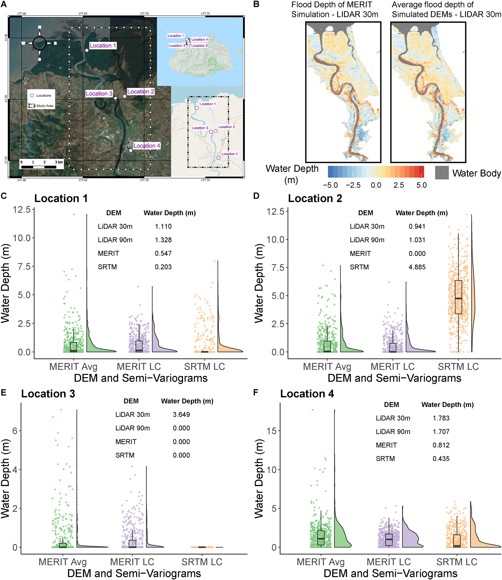
Maximum flood water depth at four locations in Ba, Fiji for a 50-year return period event. (A) Overview of study area, with locations of four random locations to investigate differences in water depth. (B) Average flood depth for models run with MERIT DEM and simulated versions of the MERIT DEM simulated using semi-variograms per landcover class against the LIDAR 30 m model. (C) Maximum water depth distribution of each DEM ensemble simulated by different sets of semi-variograms for location 1. (D) Maximum water depth distribution of each DEM ensemble simulated by different sets of semi-variograms for location 2. (E) Maximum water depth distribution of each DEM ensemble simulated by different sets of semi-variograms for location 3. (F) Maximum water depth distribution of each DEM ensemble simulated by different sets of semi-variograms for location 4. MERIT Avg refers to MERIT DEM simulated using an ‘average’ floodplain semi-variogram, MERIT LC refers to MERIT DEM simulated using semi-variograms by landcover class, SRTM LC refers to SRTM DEM simulated using semi-variograms by landcover class.
Future Directions
In this article, we have attempted to reinvigorate the idea of DEM simulation and highlight its value for flood studies. Despite repeated calls to produce a new high-accuracy open access global DEM (Schumann et al., 2014; Simpson et al., 2015), this unfortunately does not seem forthcoming. Ever-increasing computing power has made even global flood simulations possible (Sampson et al., 2015), while flood modelers also often run multiple models to explore model parameter sensitivities. However, the impact of DEM error has been largely overlooked in lieu of a lack of suitable stochastic DEM data. DEM simulation overcomes this restriction, making it possible for flood modelers to use a catalog of DEMs. Working in tandem with systematic DEM editing (e.g., MERIT), DEM simulation can fill the gap until a much-needed new high-accuracy open access DEM is produced. Even when this long-awaited DEM is eventually produced, DEM simulation will still be an invaluable approach for exploring the effect of DEM error in flood inundation estimates as long as good estimates of the spatial error structure can be made across a sufficient number of locations. We therefore encourage scientists to embrace geostatistics to simulate DEM ensembles and call for increased reporting of spatial dependence by DEM vendors and scientists alike.
Statements
Data availability statement
The MERIT dataset can be downloaded after sending a permission request to the developer (Dai Yamazaki, yamadai@rainbow.iis.u-tokyo.ac.jp) from http://hydro.iis.u-tokyo.ac.jp/~yamadai/MERIT_DEM/, and is free for research and education purposes. SRTM data can be freely downloaded from https://earthexplorer.usgs.gov/. The LiDAR dataset is available from The Secretariat of the Pacific Community′s Applied Geoscience and Technology Division (SPC SOPAC). LISFLOOD-FP is available for non-commercial purposes from http://www.bristol.ac.uk/geography/research/hydrology/models/lisflood/downloads/. The code to simulate DEMs can be found at https://github.com/laurencehawker/demgenerator.
Author contributions
LH wrote the article and carried out the data analysis. PB, JN, and JR reviewed and provided comments on various drafts as well as advised on the analysis work.
Funding
LH was funded as part of the Water Informatics Science and Engineering Center for Doctoral Training (WISE CDT) under a grant from the Engineering and Physical Sciences Research Council (EPSRC), grant number EP/L016214/1. PB was supported by a Leverhulme Research Fellowship and Royal Society Wolfson Research Merit award.
Acknowledgments
We would like to thank Leanne Archer at the University of Bristol for her work on the flood model for Ba and Dai Yamazaki for his help with the MERIT dataset. The DEMsimulation R package is available at https://github.com/laurencehawker/DEMsimulation.
Conflict of interest
The authors declare that the research was conducted in the absence of any commercial or financial relationships that could be construed as a potential conflict of interest.
References
1
ArcherL.NealJ. C.BatesP. C.HouseJ. I. (2018). Comparing TanDEM-X data with frequently-used DEMs for Flood inundation modelling.Water Res. Res.10.1029/2018WR023688
2
AndersonJ. L. (1996). A method for producing and evaluating probabilistic forecasts from ensemble model integrations.J. Clim.91518–1530. 10.1175/1520-0442(1996)009<1518:AMFPAE>2.0.CO;2
3
BarnesR.LehmanC.MullaD. (2014). Priority-flood: an optimal depression-filling and watershed-labeling algorithm for digital elevation models.Comput. Geosci.62117–127. 10.1016/j.cageo.2013.04.024
4
BaterC. W.CoopsN. C. (2009). Evaluating error associated with lidar-derived DEM interpolation.Comput. Geosci.35289–300. 10.1016/j.cageo.2008.09.001
5
BaughC. A.BatesP. D.SchumannG.TriggM. A. (2013). SRTM vegetation removal and hydrodynamic modeling accuracy.Water Resour. Res.495276–5289. 10.1002/wrcr.20412
6
BhuyianM. N. M.KalyanapuA. (2018). Accounting digital elevation uncertainty for flood consequence assessment.J. Flood Risk Manag.11S1051–S1062. 10.1111/jfr3.12293
7
BurroughP. A.McDonnellR. A. (1998). Principles of Geographical Information Systems.Oxford: Oxford University Press.
8
CallowJ. N.Van NielK. P.BoggsG. S. (2007). How does modifying a DEM to reflect known hydrology affect subsequent terrain analysis?J. Hydrol.33230–39. 10.1016/j.jhydrol.2006.06.020
9
CarabajalC. C.HardingD. J. (2006). SRTM C-Band and ICESat laser altimetry elevation comparisons as a function of tree cover and relief.Photogramm. Eng. Remote Sensing72287–298. 10.14358/PERS.72.3.287
10
CarlisleB. H. (2005). Modelling the spatial distribution of DEM error.Trans. GIS9521–540. 10.1111/j.1467-9671.2005.00233.x
11
ChenH.LiangQ.LiuY.XieS. (2018). Hydraulic correction method (HCM) to enhance the efficiency of SRTM DEM in flood modeling.J. Hydrol.55956–70. 10.1016/j.jhydrol.2018.01.056
12
CoveneyS.RobertsK. (2017). Lightweight UAV digital elevation models and orthoimagery for environmental applications: data accuracy evaluation and potential for river flood risk modelling.Int. J. Remote Sensing383159–3180. 10.1080/01431161.2017.1292074
13
CrippenR.BuckleyS.AgramP.BelzE.GurrolaE.HensleyS.et al (2016). Nasadem global elevation model: methods and progress.ISPRS Int. Arch. Photogramm. Remote Sensing Spat. Inf. Sci.XLI-B4125–128. 10.5194/isprsarchives-XLI-B4-125-2016
14
DarnellA. R.TateN. J.BrunsdonC. (2008). Improving user assessment of error implications in digital elevation models.Comput. Environ. Urban Syst.32268–277. 10.1016/j.compenvurbsys.2008.02.003
15
DavisT. J.KellerC. P. (1997). Modelling uncertainty in natural resource analysis using fuzzy sets and Monte Carlo simulation: slope stability prediction.Int. J. Geogr. Inf. Sci.11409–434. 10.1080/136588197242239
16
de FerrantiJ. (2014). Viewfinder Panorama. Available at: http://www.viewfinderpanoramas.org/dem3.html
17
DesmetP. J. J. (1997). Effects of interpolation errors on the analysis of DEMs.Earth Surf. Process. Landf.22563–580. 10.1002/(SICI)1096-9837(199706)22:6<563::AID-ESP713>3.0.CO;2-3
18
DeutschC. V.JournelA. G. (1998). GSLIB: Geostatistical Software Library and User’s Guide.New York, NY: Oxford University Press.
19
DottoriF.Di BaldassarreG.TodiniE. (2013). Detailed data is welcome, but with a pinch of salt: accuracy, precision, and uncertainty in flood inundation modeling.Water Resour. Res.496079–6085. 10.1002/wrcr.20406
20
EndrenyT. A.WoodE. F. (2001). Representing elevation uncertainty in runoff modelling and flowpath mapping.Hydrol. Process.152223–2236. 10.1002/hyp.266
21
EttritchG.HardyA.BojangL.CrossD.BuntingP.BrewerP. (2018). Enhancing digital elevation models for hydraulic modelling using flood frequency detection.Remote Sens. Environ.217506–522. 10.1016/j.rse.2018.08.029
22
FalorniG.TelesV.VivoniE. R.BrasR. L.AmaratungaK. S. (2005). Analysis and characterization of the vertical accuracy of digital elevation models from the Shuttle Radar Topography Mission.J. Geophys. Res.110:F02005. 10.1029/2003jf000113
23
FarrT. G.RosenP. A.CaroE.CrippenR.DurenR.HensleyS.et al (2007). The shuttle radar topography mission.Rev. Geophys.45:RG2004. 10.1029/2005rg000183
24
FewtrellT. J.BatesP. D.HorrittM.HunterN. M. (2008). Evaluating the effect of scale in flood inundation modelling in urban environments.Hydrol. Process.225107–5118. 10.1002/hyp.7148
25
FewtrellT. J.DuncanA.SampsonC. C.NealJ. C.BatesP. D. (2011). Benchmarking urban flood models of varying complexity and scale using high resolution terrestrial LiDAR data.Phys. Chem. Earth Parts A/B/C36281–291. 10.1016/j.pce.2010.12.011
26
FisherP. F. (1991). First experiments in viewshed uncertainty: the accuracy of the viewshed area.Photogramm. Eng. Remote Sensing571321–1327.
27
FisherP. F.TateN. (2006). Causes and consequences of error in digital elevation models.Prog. Phys. Geogr.30467–489. 10.1191/0309133306pp492ra
28
GambaP.Dell AcquaF.HoushmandB. (2002). SRTM data characterization in urban areas.Int. Arch. Photogramm. Remote Sensing Spat. Inf. Sci.3455–58.
29
GhuffarS. (2018). DEM generation from multi satellite planetscope imagery.Remote Sens.10:1462. 10.3390/rs10091462
30
GoovaertsP. (1997). Geostatistics for Natural Resource Evaluation.Oxford: Oxford University Press.
31
GuoQ.LiW.YuH.AlvarezO. (2010). Effects of topographic variability and lidar sampling density on several DEM interpolation methods.Photogramm. Eng. Remote Sensing6701–712. 10.14358/PERS.76.6.701
32
HamillT. M. (2001). Interpretation of rank histograms for verifying ensemble forecasts.Mon. Weather Rev.129550–560. 10.1175/1520-0493(2001)129<0550:IORHFV>2.0.CO;2
33
HamillT. M.ColucciS. J. (1997). Verification of Eta–RSM short-range ensemble forecasts.Mon. Weather Rev.1251312–1327. 10.1175/1520-0493(1997)125<1312:VOERSR>2.0.CO;2
34
HawkerL. P.RougierJ.NealJ.BatesP.ArcherL.YamazakiD. (2018). Implications of simulating global digital elevation models for flood inundation studies.Water Resour. Res.547910–7928. 10.1029/2018wr023279
35
HellwegerF. (1997). AGREE - DEM Surface Reconditioning System.Austin, TX: University of Texas Austin.
36
HirtC. (2018). Artefact detection in global digital elevation models (DEMs): the Maximum Slope Approach and its application for complete screening of the SRTM v4.1 and MERIT DEMs.Remote Sens. Environ.20727–41. 10.1016/j.rse.2017.12.037
37
HoftonM.DubayahR.BlairJ. B.RabineD. (2006). Validation of SRTM elevations over vegetated and non-vegetated terrain using medium footprint lidar.Photogramm. Eng. Remote Sensing72279–285. 10.14358/PERS.72.3.279
38
HolmesK. W.ChadwickO. A.KydriakidisP. C. (2000). Error in a USGS 30-meter digital elevation model and its impact on terrain modelling.J. Hydrol.233154–173. 10.1016/S0022-1694(00)00229-8
39
HorrittM.BatesP. (2002). Evaluation of 1D and 2D numerical models for predicting river flood inundation.J. Hydrol.26887–99. 10.1016/S0022-1694(02)00121-X
40
HorrittM. S.BatesP. (2001). Effects of spatial resolution on a raster based model of flood flow.J. Hydrol.253239–249. 10.1016/S0022-1694(01)00490-5
41
HuZ.PengJ.HouY.ShanJ. (2017). Evaluation of recently released open global digital elevation models of Hubei, China.Remote Sens.9:262. 10.3390/rs9030262
42
HunterG. J.GoodchildM. F. (1997). Modelling the uncertainty of slope and aspect derived from spatial databases.Geophys. Anal.2935–50.
43
HutchinsonM. F. (1989). A new procedure for gridding elevation and stream line data with automatic removal of spurious pits.J. Hydrol.106211–232. 10.1016/0022-1694(89)90073-5
44
HutchinsonM. F.GallantJ. C. (2000). “Digital elevation models and representation of terrain shape,” inTerrain Analysis: Principles and Applications, edsWilsonJ. P.GallantJ. C. (New York, NY: John Wiley and Sons), 29–50.
45
InterMap (2018). NextMap World 10. Available at: https://www.intermap.com/data/nextmap
46
JanuchowskiS. R.PresseyR. L.VanDerWalJ.EdwardsA. (2010). Characterizing errors in digital elevation models and estimating the financial costs of accuracy.Int. J. Geogr. Inf. Sci.241327–1347. 10.1080/13658811003591680
47
JarihaniA. A.CallowJ. N.McVicarT. R.Van NielT. G.LarsenJ. R. (2015). Satellite-derived Digital Elevation Model (DEM) selection, preparation and correction for hydrodynamic modelling in large, low-gradient and data-sparse catchments.J. Hydrol.524489–506. 10.1016/j.jhydrol.2015.02.049
48
JolliffeI. T.PrimoC. (2008). Evaluating rank histograms using decompositions of the chi-square test statistic.Mon. Weather Rev.1362133–2139. 10.1175/2007mwr2219.1
49
KomiK.NealJ.TriggM. A.DiekkrügerB. (2017). Modelling of flood hazard extent in data sparse areas: a case study of the Oti River basin, West Africa.J. Hydrol. Reg. Stud.10122–132. 10.1016/j.ejrh.2017.03.001
50
KulpS. A.StraussB. H. (2018). CoastalDEM: a global coastal digital elevation model improved from SRTM using a neural network.Remote Sens. Environ.206231–239. 10.1016/j.rse.2017.12.026
51
KydriakidisP. C.ShortridgeA.GoodchildM. F. (1999). Geostatistics for conflation and accuracy assessment of digital elevation models.Int. J. Geogr. Inf. Sci.13677–707. 10.1080/136588199241067
52
LaLondeT.ShortridgeA.MessinaJ. (2010). The influence of land cover on shuttle radar topography mission (SRTM) elevations in low-relief areas.Trans. GIS14461–479. 10.1111/j.1467-9671.2010.01217.x
53
LehnerB.VerdinK.JarvisA. (2008). New global hydrography derived from spaceborne elevation data.EOS Transa. Am. Geophys. Union8993–94. 10.1029/2008EO100001
54
LiJ.WongD. W. S. (2010). Effects of DEM sources on hydrologic applications.Comput. Environ. Urban Syst.34251–261. 10.1016/j.compenvurbsys.2009.11.002
55
MartzL. W.GarbrechtJ. (1999). An outlet breaching algorithm for the treatment of closed depressions in a raster DEM.Comput. Geosci.25835–844. 10.1016/S0098-3004(99)00018-7
56
MillerC. L.LaflammeR. A. (1958). The Digital Terrain Model- Theory & Application.Cambridge, MA: MIT Photogrammetry Laboratory.
57
MurilloM. L.HunterG. J. (1997). Assessing uncertainty due to elevation error in a landslide susceptibility model.Trans. GIS2289–298. 10.1111/j.1467-9671.1997.tb00058.x
58
NealJ.SchumannG.BatesP. (2012). A subgrid channel model for simulating river hydraulics and floodplain inundation over large and data sparse areas.Water Resour. Res.48:W11506. 10.1029/2012wr012514
59
NealJ. C.BatesP. D.FewtrellT. J.HunterN. M.WilsonM. D.HorrittM. S. (2009). Distributed whole city water level measurements from theCarlisle, 2005 urban flood event and comparison with hydraulic model simulations.J. Hydrol.36842–55. 10.1016/j.jhydrol.2009.01.026
60
OksanenJ.SarjakoskiT. (2005). Error propagation of DEM-based surface derivatives.Comput. Geosci.311015–1027. 10.1016/j.cageo.2005.02.014
61
O’LoughlinF. E.PaivaR. C. D.DurandM.AlsdorfD. E.BatesP. D. (2016). A multi-sensor approach towards a global vegetation corrected SRTM DEM product.Remote Sens. Environ.18249–59. 10.1016/j.rse.2016.04.018
62
PhamH. T.MarshallL.JohnsonF.SharmaA. (2018). A method for combining SRTM DEM and ASTER GDEM2 to improve topography estimation in regions without reference data.Remote Sens. Environ.210229–241. 10.1016/j.rse.2018.03.026
63
PinelS.BonnetM.-P.Santos Da SilvaJ.MoreiraD.CalmantS.SatgéF.et al (2015). Correction of interferometric and vegetation biases in the SRTMGL1 spaceborne DEM with hydrological conditioning towards improved hydrodynamics modeling in the Amazon basin.Remote Sens.716108–16130. 10.3390/rs71215822
64
Planet Observer (2017). PlanetDEM 30 Plus. Available at: https://www.planetobserver.com/products/planetdem/planetdem-30/
65
RaaflaubL. D.CollinsM. J. (2006). The effect of error in gridded digital elevation models on the estimation of topographic parameters.Environ. Model. Softw.21710–732. 10.1016/j.envsoft.2005.02.003
66
RexerM.HirtC. (2014). Comparison of free high resolution digital elevation data sets (ASTER GDEM2, SRTM v2.1/v4.1) and validation against accurate heights from the Australian National Gravity Database.Aust. J. Earth Sci.61213–226. 10.1080/08120099.2014.884983
67
RizzoliP.MartoneM.GonzalezC.WecklichC.Borla TridonD.BräutigamB.et al (2017). Generation and performance assessment of the global TanDEM-X digital elevation model.ISPRS J. Photogramm. Remote Sensing132119–139. 10.1016/j.isprsjprs.2017.08.008
68
RobinsonN.RegetzJ.GuralnickR. P. (2014). EarthEnv-DEM90: a nearly-global, void-free, multi-scale smoothed, 90m digital elevation model from fused ASTER and SRTM data.ISPRS J. Photogramm. Remote Sensing8757–67. 10.1016/j.isprsjprs.2013.11.002
69
RodriguezE.MorrisC. S.BelzJ. E. (2006). A global assessment of the SRTM performance.Photogramm. Eng. Remote Sensing72249–260. 10.14358/PERS.72.3.249
70
SaksenaS.MerwadeV. (2015). Incorporating the effect of DEM resolution and accuracy for improved flood inundation mapping.J. Hydrol.530180–194. 10.1016/j.jhydrol.2015.09.069
71
SampsonC. C.SmithA. M.BatesP. D.NealJ. C.AlfieriL.FreerJ. E. (2015). A high-resolution global flood hazard model.Water Resour. Res.517358–7381. 10.1002/2015wr016954
72
SampsonC. C.SmithA. M.BatesP. D.NealJ. C.TriggM. A. (2016). Perspectives on open access high resolution digital elevation models to produce global flood hazard layers.Front. Earth Sci.3:85. 10.3389/feart.2015.00085
73
SaundersW. (1999). “Preparation of DEMs for use in environmental modeling analysis,” inProceedings of the ESRI User Conference, (San Diego, CA: ESRI).
74
SavageJ. T. S.BatesP.FreerJ.NealJ.AronicaG. (2016a). When does spatial resolution become spurious in probabilistic flood inundation predictions?Hydrol. Process.302014–2032. 10.1002/hyp.10749
75
SavageJ. T. S.PianosiF.BatesP.FreerJ.WagenerT. (2016b). Quantifying the importance of spatial resolution and other factors through global sensitivity analysis of a flood inundation model.Water Resour. Res.529146–9163. 10.1002/2015wr018198
76
SchumannG. J. P.BatesP.NealJ.AndreadisK. M. (2014). Technology: fight floods on a global scale.Nature507:169. 10.1038/507169e
77
ShortridgeA. (2006). Shuttle radar topography mission elevation data error and its relationship to land cover.Cartogr. Geogr. Inf. Sci.3365–75. 10.1559/152304006777323172
78
ShortridgeA.MessinaJ. (2011). Spatial structure and landscape associations of SRTM error.Remote Sens. Environ.1151576–1587. 10.1016/j.rse.2011.02.017
79
SimpsonA. L.BalogS.MollerD. K.StraussB. H.SaitoK. (2015). An urgent case for higher resolution digital elevation models in the world’s poorest and most vulnerable countries.Front. Earth Sci.3:50. 10.3389/feart.2015.00050
80
SmithM. J.ClarkC. D. (2005). Methods for the visualization of digital elevation models for landform mapping.Earth Surf. Process. Landf.30885–900. 10.1002/esp.1210
81
SuY.GuoQ.MaQ.LiW. (2015). SRTM DEM correction in vegetated mountain areas through the integration of spaceborne LiDAR, airborne LiDAR, and optical imagery.Remote Sens.711202–11225. 10.3390/rs70911202
82
SzabóG.SinghS. K.SzabóS. (2015). Slope angle and aspect as influencing factors on the accuracy of the SRTM and the ASTER GDEM databases.Phys. Chem. Earth Parts A/B/C83–84, 137–145. 10.1016/j.pce.2015.06.003
83
TadonoT.IshidaH.OdaF.NaitoS.MinakawaK.IwamotoH. (2014). Precise global DEM generation by ALOS PRISM.ISPRS Ann. Photogramm. Remote Sensing Spat. Inf. Sci. II471–76. 10.5194/isprsannals-II-4-71-2014
84
TakakuJ.TadonoT. (2017). “Quality updates of ‘AW3D’ global DSM generated from ALOS PRISM,” inProceedings of the IEEE International Geoscience and Remote Sensing Symposium (IGARSS), (Fort Worth, TX: IEEE). 10.1109/IGARSS.2017.8128293
85
TalagrandO.VautardR.StraussB. (1997). “Evaluation of probabilistic prediction systems,” inProceedings of the Workshop on Predictability, (Reading: ECMWF).
86
TarakegnT. H.SayamaT. (2013). Correction of SRTM artefacts by fourier transform for flood inundation modelling.J. Jpn. Soc. Civ. Eng. Ser. B169:193-I. 10.2208/jscejhe.69.I_193
87
ToblerW. R. (1970). A computer movie simulating urban growth in the Detroit Region.Econ. Geogr.46234–240. 10.2307/143141
88
ToutinT. (2002). Impact of terrain slope and aspect on radargrammetric DEM accuracy.ISPRS J. Photogramm. Remote Sensing57228–240. 10.1016/S0924-2716(02)00123-5
89
UysalM.ToprakA. S.PolatN. (2015). DEM generation with UAV Photogrammetry and accuracy analysis in Sahitler hill.Measurement73539–543. 10.1016/j.measurement.2015.06.010
90
VereginH. (1997). The effects of vertical error in digital elevation models on the determination of flow-path direction.Cartogr. Geogr. Inf. Syst.2467–79. 10.1559/152304097782439330
91
WalkerW. S.KellndorferJ. M.PierceL. E. (2007). Quality assessment of SRTM C- and X-band interferometric data: implications for the retrieval of vegetation canopy height.Remote Sens. Environ.106428–448. 10.1016/j.rse.2006.09.007
92
WechslerS. P. (2003). Perceptions of digital elevation model uncertainty by DEM users.URISA J.1557–64.
93
WechslerS. P. (2007). Uncertainties associated with digital elevation models for hydrologic applications: a review.Hydrol. Earth Syst. Sci.111481–1500. 10.5194/hess-11-1481-2007
94
WeydahlD. J.SagstuenJ.DickØ. B.RønningH. (2007). SRTM DEM accuracy assessment over vegetated areas in Norway.Int. J. Remote Sens.283513–3527. 10.1080/01431160600993447
95
WilsonM. D.AtkinsonP. M. (2005). “Prediction uncertainty in elevation and its effect on flood inundation modelling,” inGeodynamics, edsAtkinsonP. M.FoodyG. M.DarbyS.WuF. (Andover, MN: CRC Press), 185–202.
96
WiseS. (2000). Assessing the quality for hydrological applications of digital elevation models derived from contours.Hydrol. Process.141909–1929. 10.1002/1099-1085(20000815/30)14:11/12<1909::AID-HYP45>3.0.CO;2-6
97
WiseS. (2007). Effect of differing DEM creation methods on the results from a hydrological model.Comput. Geosci.331351–1365. 10.1016/j.cageo.2007.05.003
98
WiseS. (2011). Cross-validation as a means of investigating DEM interpolation error.Comput. Geosci.37978–991. 10.1016/j.cageo.2010.12.002
99
WoodrowK.LindsayJ. B.BergA. A. (2016). Evaluating DEM conditioning techniques, elevation source data, and grid resolution for field-scale hydrological parameter extraction.J. Hydrol.5401022–1029. 10.1016/j.jhydrol.2016.07.018
100
WuS.LiJ.HuangG. H. (2008). A study on DEM-derived primary topographic attributes for hydrologic applications: sensitivity to elevation data resolution.Appl. Geogr.28210–223. 10.1016/j.apgeog.2008.02.006
101
YamazakiD.IkeshimaD.TawatariR.YamaguchiT.O’LoughlinF.NealJ. C.et al (2017). A high-accuracy map of global terrain elevations.Geophys. Res. Lett.45844–5853. 10.1002/2017gl072874
102
YanK.TarpanelliA.BalintG.MoramarcoT.BaldassarreG. D. (2015). Exploring the potential of SRTM topography and radar altimetry to support flood propagation modeling: Danube case study.J. Hydrol. Eng.20:04014048. 10.1061/(asce)he.1943-5584.0001018
103
YueL.ShenH.ZhangL.ZhengX.ZhangF.YuanQ. (2017). High-quality seamless DEM generation blending SRTM-1, ASTER GDEM v2 and ICESat/GLAS observations.ISPRS J. Photogramm. Remote Sensing12320–34. 10.1016/j.isprsjprs.2016.11.002
104
ZhaoX.SuY.HuT.ChenL.GaoS.WangR.et al (2018). A global corrected SRTM DEM product for vegetated areas.Remote Sens. Lett.9393–402. 10.1080/2150704x.2018.1425560
Summary
Keywords
digital elevation models, open-access, geostatistics, flood, stochastic simulation, floodplains, hazards
Citation
Hawker L, Bates P, Neal J and Rougier J (2018) Perspectives on Digital Elevation Model (DEM) Simulation for Flood Modeling in the Absence of a High-Accuracy Open Access Global DEM. Front. Earth Sci. 6:233. doi: 10.3389/feart.2018.00233
Received
25 July 2018
Accepted
30 November 2018
Published
18 December 2018
Volume
6 - 2018
Edited by
Matthew McCabe, King Abdullah University of Science and Technology, Saudi Arabia
Reviewed by
Salvatore Manfreda, University of Basilicata, Italy; Ben Jarihani, University of the Sunshine Coast, Australia
Updates
Copyright
© 2018 Hawker, Bates, Neal and Rougier.
This is an open-access article distributed under the terms of the Creative Commons Attribution License (CC BY). The use, distribution or reproduction in other forums is permitted, provided the original author(s) and the copyright owner(s) are credited and that the original publication in this journal is cited, in accordance with accepted academic practice. No use, distribution or reproduction is permitted which does not comply with these terms.
*Correspondence: Laurence Hawker, Laurence.hawker@bristol.ac.uk
This article was submitted to Hydrosphere, a section of the journal Frontiers in Earth Science
Disclaimer
All claims expressed in this article are solely those of the authors and do not necessarily represent those of their affiliated organizations, or those of the publisher, the editors and the reviewers. Any product that may be evaluated in this article or claim that may be made by its manufacturer is not guaranteed or endorsed by the publisher.