Utilizing Flood Inundation Observations to Obtain Floodplain Topography in Data-Scarce Regions

Introduction

Prediction of inundation extents from flood models is an indispensable source of information for assessing flood risk in the context of hazard studies, but inundation prediction accuracy is often limited by the quality of topographic data available globally. Topographic data, generally in the form of digital elevation models (DEMs), are the primary input data for flood inundation modeling. Airborne light detection and ranging (lidar) DEMs offer the best horizontal resolution and vertical accuracy. However, high resolution lidar DEMs are not available globally and are expensive to obtain. Globally, the best available DEMs are obtained from satellite data: the shuttle radar topography mission (SRTM, spatial resolution 30 m) (Rodriguez et al., 2006) and multi-error-removed improved-terrain (MERIT, spatial resolution 90 m) (Yamazaki et al., 2017) DEM are a few examples of freely available DEMs. The global average for vertical relative error in SRTM is about 6 m (Rodriguez et al., 2006). TanDEM-X DEM produced by DLR (German Aerospace Center) has better spatial resolution (10–12 m) and vertical accuracy (∼2 m) (Krieger et al., 2006; Eineder et al., 2012). However, it is a commercial product and is not freely available. Because the vertical inaccuracies of the SRTM DEM, flood inundation modeling using SRTM produces spatial inconsistencies (Sanders, 2007; Yamazaki et al., 2012; Yan et al., 2015; Fernández et al., 2016; Sampson et al., 2016). Hence, these DEMs are not suitable for flood simulations as they do not represent the topography well (Sanders, 2007). There have been calls to produce global scale high resolution DEMs because of its impact on emergency services and scientific research (Schumann et al., 2014).

Spaceborne remote sensing observations of inundation extent contain indirect information about floodplain topography. Remotely sensed data is widely used to study floods (Schumann and Domeneghetti, 2016) for applications such as flood risk assessment, emergency flood response, and flood mapping, but inference of floodplain topography from inundation has rarely been attempted; Mason et al. (2016) is an example of one such study. Spatiotemporal inundation patterns in floodplains are responses to a combination of factors and input variables like flow rate in the river channels, soil type, vegetation, etc.: floodplain topography determines where floodwaters flow after rivers flood their banks. For this reason, inundation patterns contain indirect information about floodplain topography. As a specific example, the boundaries of flood inundation are essentially the contours of ground elevation, if the water level is assumed to be flat (this idea can easily be extended to account for river slope, as well). Using inundation “contours” in this way is the inverse of the well-known body of the literature that uses inundation intersected with a high precision DEM to infer water levels (Matgen et al., 2007; Cohen et al., 2018). It is intuitive that these contours could be used to constrain relative variations in floodplain topography: for example, noisy elevations could be smoothed by averaging along inundation edges. Mason et al. (2016) used synthetic aperture radar (SAR) derived flood extents to improve the height accuracy in TanDEM-X DEM. They tested the method in a region where the errors had a mean and standard deviation of ∼ 0.5 and ∼2 m, respectively. The mean difference between TanDEM-X and lidar DEM reduced from 0.5 to 0.3 m, and their standard deviation reduced from 2 to 1.2 m. However, it is not certain the method would work for regions with higher height errors, like SRTM, which has mean and standard deviation of errors in the range of ∼ 1.2 and ∼ 4 m, respectively.

Because inundation images reflect the complex flow paths that water takes during flooding events that can only be captured by flood models, methods such as Mason et al. (2016) (referred to as “smoothing methods,” hereafter) are unlikely to extract all possible topographic information from inundation imagery. Because two-dimensional flood models encapsulate floodplain processes, it is natural to attempt to use such models to help extract topographic information from inundation. Indeed, the objective here is to infer floodplain topography using inundation maps, while flood models do the inverse: predict inundation using floodplain topography. Thus, this is a classic example of an “inverse problem” (Yeh, 1986). Data assimilation is a technique that can be used to solve inverse problems; assimilation combines measurements and models to produce an estimate of the system which is better than just the measurement or model alone.

To our knowledge, assimilation has not been used to estimate floodplain DEMs, though related work has been done. Durand et al. (2008) assimilated water surface elevation observations along with LISFLOOD-FP hydrodynamic model to estimate channel bathymetry. Observations from SAR images of river inundation were assimilated with 2-D shallow water equations to identify optimal Manning’s coefficients (Lai and Monnier, 2009; Hostache et al., 2010; Monnier et al., 2016). One obvious impediment to using flood models to infer floodplain topography is the high dimensionality of the problem: in principle, the elevation value for each grid cell in the floodplain model must be estimated. An additional consideration is that flood models are computationally expensive, and many assimilation algorithms require either repeated model runs or ensembles of runs. A final concern is the high degree of non-linearity between the observed inundation and the floodplain topography, as some approaches [e.g., the ensemble-based assimilation of Durand et al. (2008)] are based on linear estimation theory. The non-linearity can be accounted for by using a so-called “Particle Batch Smoother” (PBS), as described in Margulis et al. (2015), which is a non-Gaussian estimator that directly approximates Bayes theorem.

In the present study, we present and test (using synthetic observations) a new algorithm designed to infer floodplain topography using globally available DEMs and inundation imagery. The algorithm consists of two steps: smoothing and data assimilation, that capitalize on the strengths of each method.

Experiment Design

We tested our algorithm for a synthetic case of small domain. This allowed us to explore the sensitivity of the algorithm to errors of various magnitude. We used the Buscot model, a tested example model distributed with LISFLOOD-FP, as our synthetic test case. LISFLOOD-FP (Bates and De Roo, 2000; Bates et al., 2010) is a raster-based inundation model. We considered the DEM used in this model as the truth. The model had a defined river channel, and the flow in it was defined by the inflow boundary condition. The flow into the channel was defined as a triangular hydrograph with a flow of 20 m³/s at time 0, 200 m³/s at its peak and back to 20 m³/s at the end of the 5-day simulation. Figure 1A shows the DEM, and Figure 1B shows the maximum flooded extent for this test case.

FIGURE 1

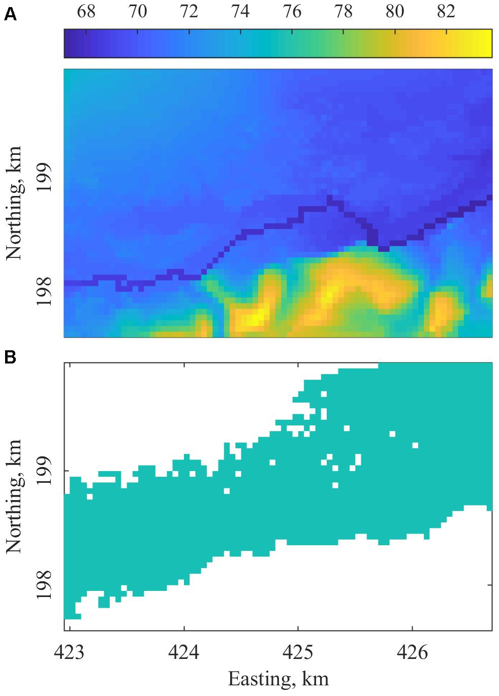
Figure 1. (A) True DEM for the Buscot case and (B) maximum flooded extent.

To obtain best results from this method, we require multiple unique flood extent observations. We used 9 flood inundation maps obtained between day 1 and peak inundation on day 3 as observations. Our primary objective was to test the efficacy of the algorithm itself, and we did not focus on studying the impact of less or more flood inundation observations. In order to focus on the effect of prior DEM error on the analysis, we did not add white noise to the classified imagery; we leave for future work how observational uncertainty and temporal revisit would impact the algorithm accuracy. Figure 2 shows flood inundation area for the simulation period, and the maps that were used as observations.

FIGURE 2

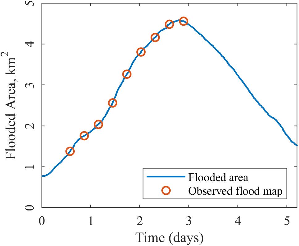
Figure 2. Flood inundation area and available flood maps.

In the design of the synthetic experiment, we attempt to simulate a realistic situation where we attempt to correct a noisy “prior” estimate of the floodplain DEM. We accomplish this by taking the DEM distributed with the Buscot model to be the “truth.” We then create a prior estimate of the DEM by adding errors to the truth. Here we chose to add spatially uncorrelated errors when creating the prior; the level of the errors varies among the various cases. We define the “nominal case” to be addition of 0.5 m bias and 1 m standard deviation of errors, which is referred to as the prior henceforth. We performed sensitivity analysis by considering 8 additional cases, by exploring bias ranging from 0.5, 1, and 2 m, and standard deviation of 1, 2, and 4 m. The case with bias of 0.5 and 2 m is similar to the TanDEM-X errors, which was used by Mason et al. (2016). The cases with bias of 1 and 2 m, and standard deviation of 4 m is similar to SRTM.

We evaluated the performance of the algorithm by calculating bias, standard deviation of DEM errors and root mean squared error (RMSE) for all the pixels modified by the algorithm. We also evaluated the DEM’s ability to predict inundation by using true positive rate (TPR), a statistical measure of binary classification. TPR is the proportion of predicted inundation area from the model that is accurate (from observations).

Materials and Methods

Our approach merges smoothing and data assimilation to better extract floodplain topography information from inundation maps. We will use the PBS concept described by Margulis et al. (2015) for a different estimation problem. The PBS is related to the Ensemble Kalman batch smoother used by Durand et al. (2008) to infer channel bathymetry from inundated area, but relies upon a fully Bayesian approach that does not assume linearity between the observations and the quantities to be estimated. The PBS represents the relationships between observations and model parameters, as well as the associated uncertainty, using a set of model simulations, which are referred to as “particles.” Each particle represents an independent random realization of the sample. The basic idea is to generate a moderately sized set of particles, where each particle is a random perturbation of the prior DEM. Here we adapt the usual PBS algorithm by first performing smoothing on each of the particles prior to the PBS estimation. Then the LISFLOOD-FP model is run on each of the smoothed particles. Finally, the PBS estimate of the DEM is computed by comparing the LISFLOOD-FP model run output of each particle to the map of inundation observation. The PBS estimate can be thought of as a weighted average of all the DEM particles, where the weights are based upon the accuracy of LISFLOOD-FP in simulating the inundation. Figure 3 shows an outline of the method we use to estimate an updated DEM using the PBS. One note of clarification: we use weighted averages in two contexts. In the first case, they are used for the smoothing elevations along flood boundaries, and they are referred to as weights (ensemble and regression). In the data assimilation step, we use particle weights to obtain the final estimate, and these weights are referred to as particle weights.

FIGURE 3

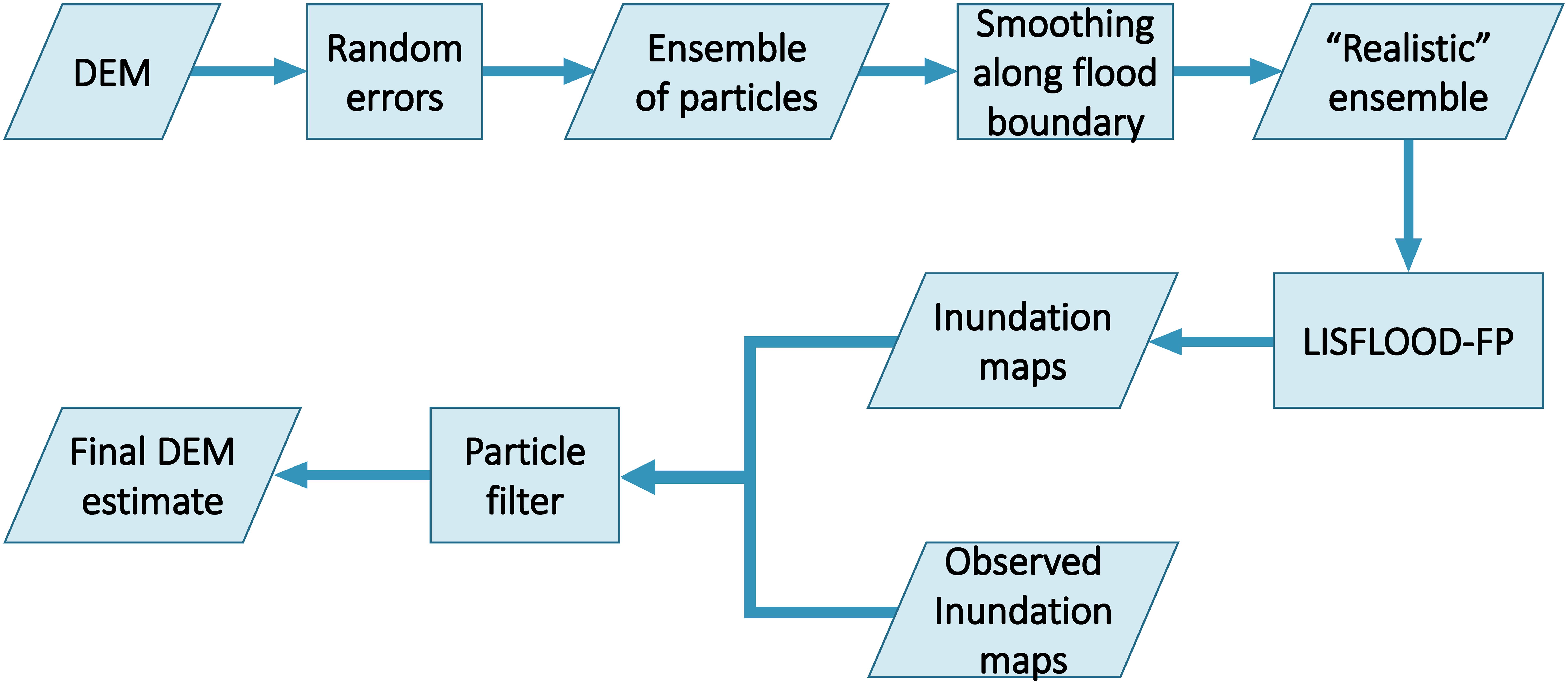
Figure 3. Outline of the methods.

Generating Particles

It has been established from empirical evidence that DEM errors are not completely random, and often have spatial correlation (Hunter and Goodchild, 1997; Fisher, 1998; Kyriakidis et al., 1999; Carlisle, 2005; Erdoǧan, 2010). Hence, we added spatially correlated errors to the prior (It should be noted that, in this implementation of a synthetic case, we created the prior by adding uncorrelated random errors to the “true” DEM.), and generated an ensemble of 50 particles. We added errors with zero mean, 1 m standard deviation and 250 m correlation length to the prior. We also added a constant bias to each particle; the constant bias was randomly generated in the same range as the bias of the prior (-0.5 to 0.5 m for the nominal case).

The set of randomly perturbed DEMs thus obtained might be inefficient as the process may generate many unrealistic DEM particles. Data assimilation style approach will require a large set of particles to capture the complex spatial pattern of topography, making the process computationally inefficient. One way to deal with this problem is to make the ensemble of particles more realistic. We make this ensemble of particles more realistic by using the process described in Section “Smoothing Along Flood Boundary”.

Smoothing Along Flood Boundary

We exploited the indirect information about elevations along the flood boundary to produce a set of realistic particles. For each particle in the ensemble, we extracted the elevations along the flood boundary. We extracted two adjacent pixels along the boundary: one flooded pixel on the edge (the “wet boundary”), and the adjacent pixel on the non-flooded side (the “dry boundary”). Then, we performed linear regression along both boundaries, considering the wet and dry boundaries separately. We consider the length along the boundary going from upstream to downstream as the independent variable and the extracted elevations as the dependent variable. We modified each particle by updating the elevations along the flood boundary as the weighted average of extracted elevations, and its regressions. By doing this, the noise in elevations along the boundary was reduced (Figure 4). The weights are expressed as the inverse of RMSE of the prior, and of the regression. We used nine flood inundation maps to perform this operation.

FIGURE 4

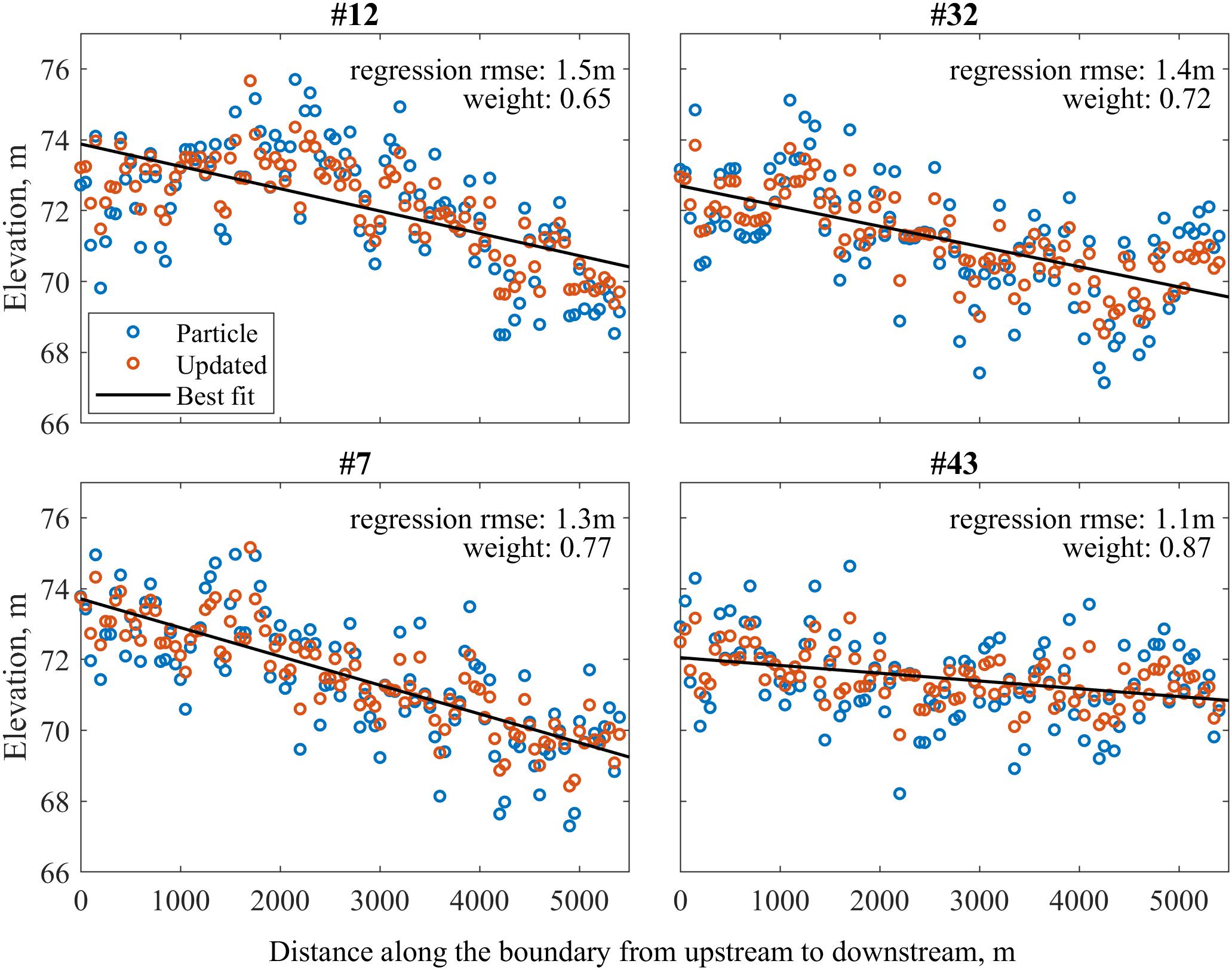
Figure 4. Elevations along the boundary for four sample ensemble members for the nominal case. Weight refers to the inverse of RMSE of the best fit line, and is used to smooth the elevations along the boundary.

We used the estimate of bias and standard deviation of errors for the prior to calculate RMSE of the prior. We use this RMSE to compute the ensemble weight, w_en, as the inverse of RMSE of the prior. For the regressed line along the boundary, the weight is defined as:

$$w_{fit,\mathrm{\hspace{0.17em}}j}=\frac{1}{rms(z_{en}-z_{fit,j})}\mathrm{\hspace{0.17em}}\mathrm{\hspace{0.17em}}\mathrm{\hspace{0.17em}}\mathrm{\hspace{0.17em}}\mathrm{\hspace{0.17em}}\mathrm{\hspace{0.17em}}\mathrm{\hspace{0.17em}}\mathrm{\hspace{0.17em}}\mathrm{\hspace{0.17em}}\mathrm{\hspace{0.17em}}\mathrm{\hspace{0.17em}}\mathrm{\hspace{0.17em}}\mathrm{\hspace{0.17em}}\mathrm{\hspace{0.17em}}\mathrm{\hspace{0.17em}}\mathrm{\hspace{0.17em}}\mathrm{\hspace{0.17em}}\mathrm{\hspace{0.17em}}\mathrm{\hspace{0.17em}}\mathrm{\hspace{0.17em}}\mathrm{\hspace{0.17em}}\mathrm{\hspace{0.17em}}\mathrm{\hspace{0.17em}}\mathrm{\hspace{0.17em}}\mathrm{\hspace{0.17em}}\mathrm{\hspace{0.17em}}\mathrm{\hspace{0.17em}}\mathrm{\hspace{0.17em}}\mathrm{\hspace{0.17em}}\mathrm{\hspace{0.17em}}\mathrm{\hspace{0.17em}}(1)$$

where w_fit,j is the regressed weight of jth particle, z_en is the elevation along flood boundary in the prior, and z_fit,j is the elevation along flood boundary in the jth particle. Figure 4 shows RMS of difference between regression (z_fit,j) and prior (z_en) elevations along the boundary, and its corresponding weight (w_fit,j) for four sample particles. The updated elevation along the flood boundary, $z_j^{+}$, is calculated as:

$$z_j^{+}=\frac{w_{en}{z}_{en,j}+w_{fit,j}{z}_{fit,j}}{w_{en}+w_{fit,j}}\mathrm{\hspace{0.17em}}\mathrm{\hspace{0.17em}}\mathrm{\hspace{0.17em}}\mathrm{\hspace{0.17em}}\mathrm{\hspace{0.17em}}\mathrm{\hspace{0.17em}}\mathrm{\hspace{0.17em}}\mathrm{\hspace{0.17em}}\mathrm{\hspace{0.17em}}\mathrm{\hspace{0.17em}}\mathrm{\hspace{0.17em}}\mathrm{\hspace{0.17em}}\mathrm{\hspace{0.17em}}\mathrm{\hspace{0.17em}}(2)$$

Figure 4 shows the elevations along the boundary for the particle, regressed and updated elevations for four sample particles in the nominal case. The flood boundary of each ensemble member was replaced with this value of $z_j^{+}$ from that particle to obtain an updated set of particles.

When we modify elevations along the observed flood boundary, we introduce sub-optimality into the analysis, because the errors in the smoothed DEMs are now dependent on errors in the observations. Thus the errors in the LISFLOOD-FP predictions are also correlated with the errors in the observations, whereas the PBS assumes that they are not correlated. However, we assume that the degree of sub-optimality introduced by using the observations is relatively small compared to the large errors in the prior DEM.

Data Assimilation

We ran a forward simulation of LISFLOOD-FP using the updated particles ($z_j^{+}$) to obtain inundation maps for each particle. All the parameters (except the DEM) in the model were the same as in the simulation using “true” DEM. The inundation maps from this set of simulations were used along with observed inundation maps using PBS (Durand et al., 2008; Margulis et al., 2015) to estimate the updated DEM. PBS is a non-Gaussian estimator which directly approximates Bayes theorem. Initially, all ensemble members are assigned equal particle weights. We evaluate the likelihood of each particle by simulating flood inundation maps, and calculating the agreement between the modeled and observed flood inundation. True positive rate (TPR) is used to define the agreement between the modeled and observed inundation. We used exponential probability distribution to update the weights. The value of the probability density function w_j at any point t_j=1-TPR_j is defined as the particle weight of the jth particle. The probability density function for exponential distribution is defined as:

$$w_j=\mathrm{\lambda }{e}^{-\mathrm{\lambda }{t}_j}\mathrm{\hspace{0.17em}}\mathrm{\hspace{0.17em}}\mathrm{\hspace{0.17em}}\mathrm{\hspace{0.17em}}\mathrm{\hspace{0.17em}}for\mathrm{\hspace{0.17em}}{t}_j>0\mathrm{\hspace{0.17em}}\mathrm{\hspace{0.17em}}\mathrm{\hspace{0.17em}}\mathrm{\hspace{0.17em}}\mathrm{\hspace{0.17em}}\mathrm{\hspace{0.17em}}\mathrm{\hspace{0.17em}}\mathrm{\hspace{0.17em}}\mathrm{\hspace{0.17em}}\mathrm{\hspace{0.17em}}\mathrm{\hspace{0.17em}}\mathrm{\hspace{0.17em}}\mathrm{\hspace{0.17em}}\mathrm{\hspace{0.17em}}\mathrm{\hspace{0.17em}}(3)$$

where t_j is the random variable, λ is a rate parameter and λ=1/µ=1/σ, µ being the expected value of the distribution and σ the standard deviation. We then update the particle weight according to its likelihood of producing accurate inundation maps. The rate parameter λ is used to represent uncertainty in observations, and we use a value of 0.1 in the current study. Here, we calibrated the value of λ for the data assimilation to produce largest error correction. This means that our confidence in observations is high. The value of λ can be modified to represent the confidence in the observations. Higher value of λ produces less contrast between weights at t equal to 0 and 1. Hence, the weights are close to each other, indicating a lower confidence in observations. The updated particle weight is proportional to the likelihood of the model predicting the observation. Particles that produce inundation maps with high agreement have large particle weights; particles that have poor agreement have small particle weights. The posterior or updated DEM is the weighted average of the prior DEMs, calculated as shown in (4).

$$DE{M}^{+}=\frac{{\displaystyle \sum w_{j}DE{M}_j^{-}}}{{\displaystyle \sum w_j}}\mathrm{\hspace{0.17em}}\mathrm{\hspace{0.17em}}\mathrm{\hspace{0.17em}}\mathrm{\hspace{0.17em}}\mathrm{\hspace{0.17em}}\mathrm{\hspace{0.17em}}\mathrm{\hspace{0.17em}}\mathrm{\hspace{0.17em}}\mathrm{\hspace{0.17em}}\mathrm{\hspace{0.17em}}\mathrm{\hspace{0.17em}}\mathrm{\hspace{0.17em}}\mathrm{\hspace{0.17em}}\mathrm{\hspace{0.17em}}(4)$$

where DEM⁺ is the updated estimate, DEM^-_j and w_j are jth particle and its particle weight of jth particle. Figure 5 shows the agreement in flood extent between the model and observations for a sample of nine particles. TPR, and the corresponding particle weight (w_j) assigned to that particle for those nine particles are shown in their respective panel in Figure 5. It can be seen that the particles that produce inundation maps with high agreement are given high particle weights, and vice versa. The final estimate DEM is obtained by using these particle weights to obtain a weighted mean of the updated ensemble of particles.

FIGURE 5

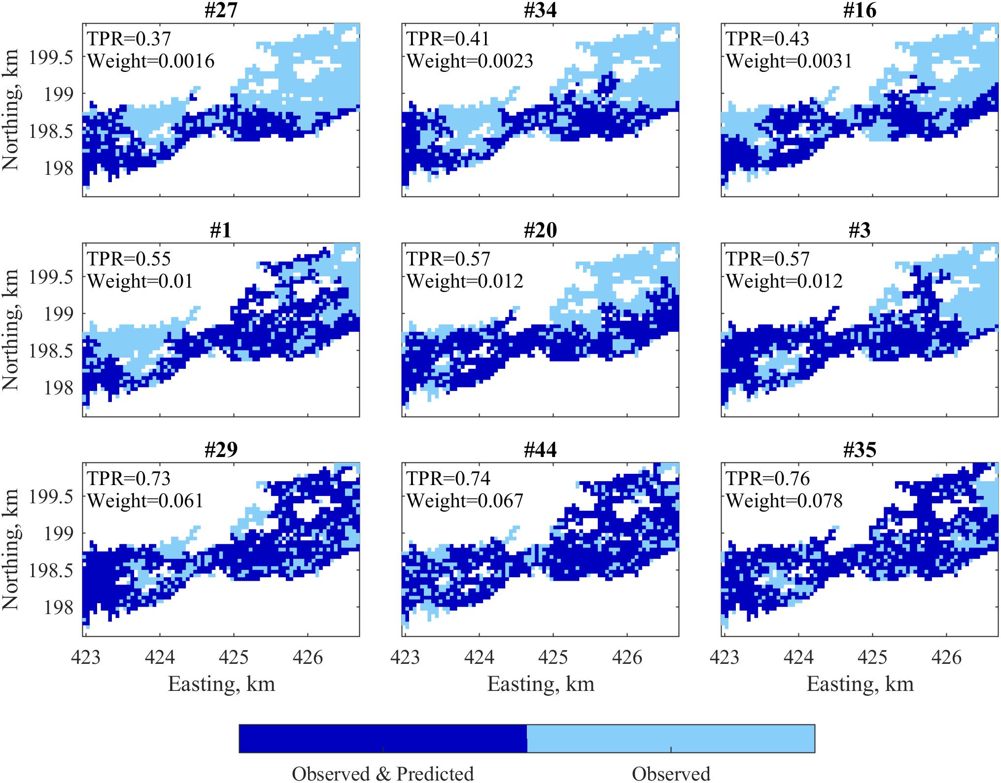
Figure 5. Agreement between observed and predicted flooded area for a sample of nine particles, and their corresponding weights for the nominal case. TPR is the true positive rate; weight refers to the particle weights assigned using the exponential distribution.

Sensitivity Analysis

In most continents, the mean SRTM error is less than 2 m, and standard deviation is ∼4 m (Rodriguez et al., 2006). To ensure that our methodology works in these ranges, we implemented the algorithm for several cases with varying levels of error mean and standard deviation in the prior. We created eight additional priors to the nominal case. The nine cases had errors of mean 0.5, 1, and 2 m, and standard deviation of 1, 2, and 4 m added to the “true” DEM. We applied the algorithm described in Section “Generating Particles, Smoothing Along Flood Boundary, and Data Assimilation” to the eight additional priors to obtain the final estimate DEM for those respective cases.

Results and Discussion

Root mean squared error for the prior for the nominal case (errors of 0.5 m mean and 1 m standard deviation) was 1.10 m. The set of particles generated from this prior had an RMSE of was 1.10 m. The RMSE of height errors along the flood boundaries reduced to 0.78 m in the updated set of particles where we smoothed elevations along the flood boundary. Table 1 shows height errors in the initial ensemble and updated ensemble of particles. After putting this modified set of particles through the PBS, the RMSE further reduced to 0.71 m. The bias reduced from 0.5 to 0.4 m and standard deviation of errors went down from 0.98 to 0.59 m.

TABLE 1

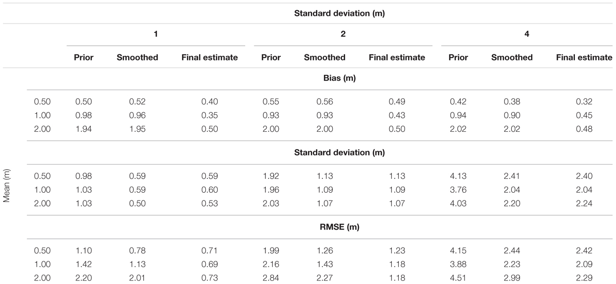
Table 1. Statistics for height errors along the flood boundary before and after smoothing.

Sensitivity analysis also showed similar trends, improving upon priors in terms of bias, standard deviation of errors and RMSE. We found that the process of smoothing did not have an effect on the bias before and after smoothing. The difference between prior bias and smoothed bias is less than 4 cm for all the cases (Table 1). However, the standard deviation of errors went down after smoothing. The standard deviation of error was reduced by 40 to 49% in all the cases (Table 1). Generally, as the standard deviation in the prior increased, the amount of reduction increased. The amount of reduction also increased as the bias in the prior increased. Table 1 shows the values of standard deviation for all the tested cases for the prior and smoothed ensembles.

When this smoothed set of particles was put through a PBS, the bias reduced in the final estimate from the prior and the smoothed ensemble. Table 1 shows the details about error for the final estimate of elevations along the flood boundary. In general, the relative reduction in bias increased as the prior’s bias increased. For the cases with 0.5 m bias, reduction in bias for the final estimate ranged between 11 and 24%. In all other cases (1 and 2 m bias), the bias reduced to 0.5 m or less. The reduction in bias ranged between 52 and 76%. However, there was no effect of the PBS on the standard deviation of error. The reduction is standard deviation of errors was less than 4 cm for all the cases (Table 1).

Figure 6 shows the histograms for errors in all tested cases. It is clear from Figure 6 that there is a reduction in bias and standard deviation of errors from the prior to the final estimate. A greater number of cells have lower errors, and the number of cells with high errors are reduced. The algorithm improved upon the prior in all the cases, and the reduction in RMSE varied from 35 to 67%.

FIGURE 6

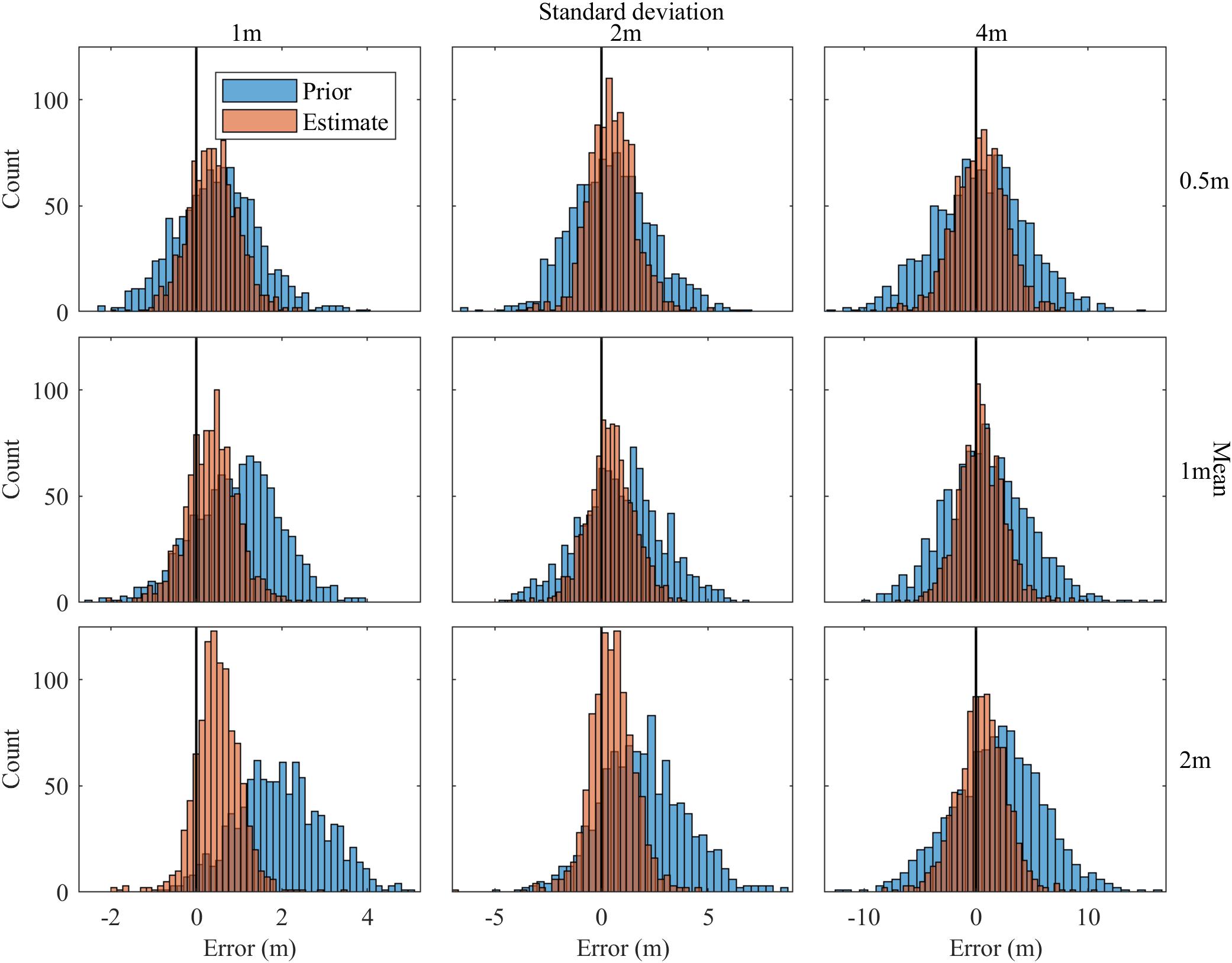
Figure 6. Error histograms for all cases.

When we used the final estimate DEMs to predict flood inundation, there was a consistent increase in TPR when compared to the prior. Figure 7 shows the predicted inundation area for the simulation period. In all the cases, the correctly predicted flood inundation area (i.e., the total area where inundation is in observation and prediction) was greater for the final estimate than the prior. Figure 8 shows the flood inundation maps obtained from the prior and final estimated DEMs for two cases. The top row shows the peak inundation maps for the case with error of 2 m mean and 1 m standard deviation on 2.3 days. The TPR goes up from 33 to 82%. The second row corresponds to the case with error of mean 2 m and standard deviation 4 m, the case we believe is similar to SRTM DEM. In this case, the TPR increases from 29 to 57%. Table 2 shows the change in TPR for peak inundation in all the cases. There was greater improvement of TPR with increase in bias of the priors. TPR for the peak inundation obtained from the final estimate DEM for all the cases with 1 m error standard deviation was greater than 82%. For the cases with 2 m error standard deviation, TPR for the peak inundation obtained from the final estimate DEM was between 63 and 75%; for cases with 4 m standard deviation of errors, it ranged between 52 and 62% (Table 2). It can be seen than there is a significant increase in TPR from prior to final estimate in all cases.

FIGURE 7

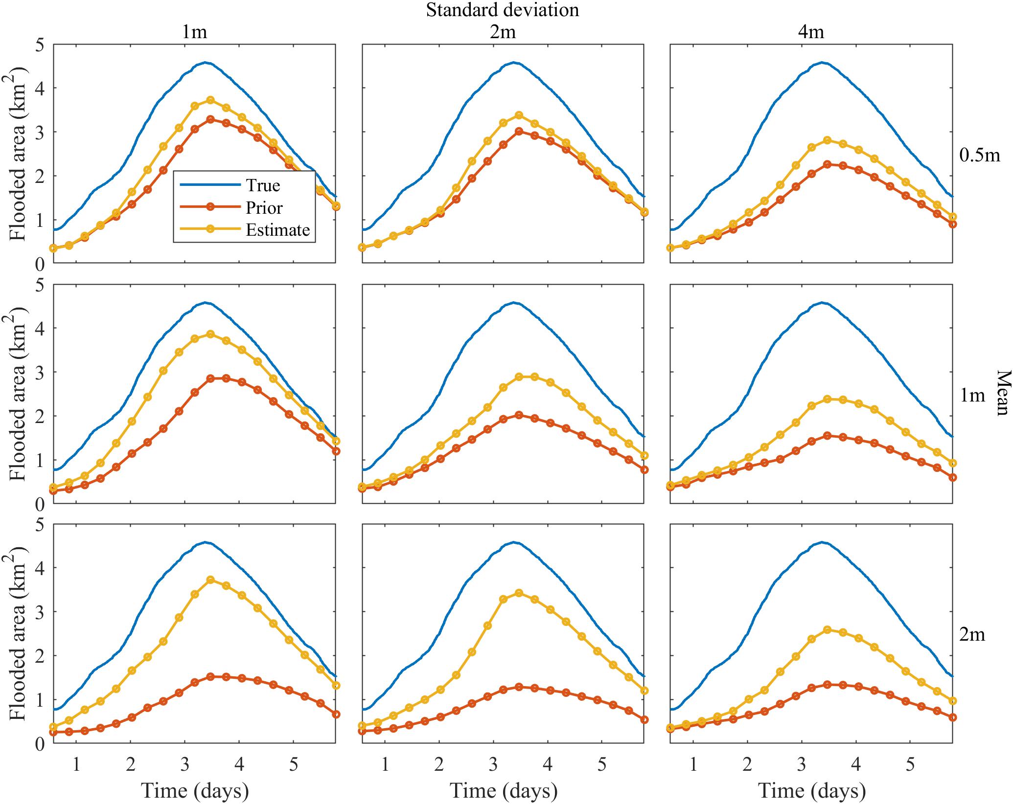
Figure 7. Total area where inundation is in both the observation and prediction for all cases.

FIGURE 8

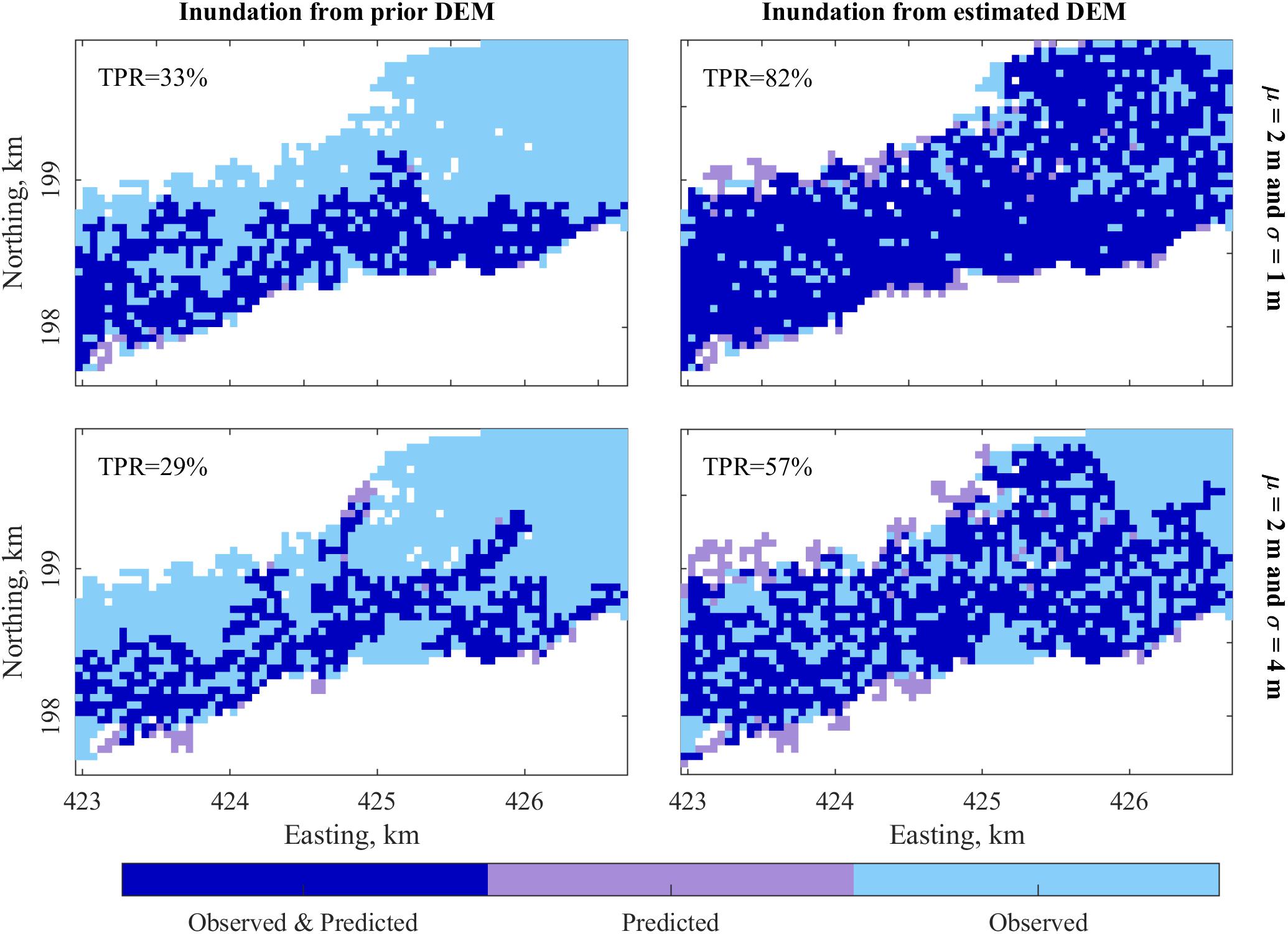
Figure 8. Predicted flood inundation from prior and estimated DEM for two cases.

TABLE 2

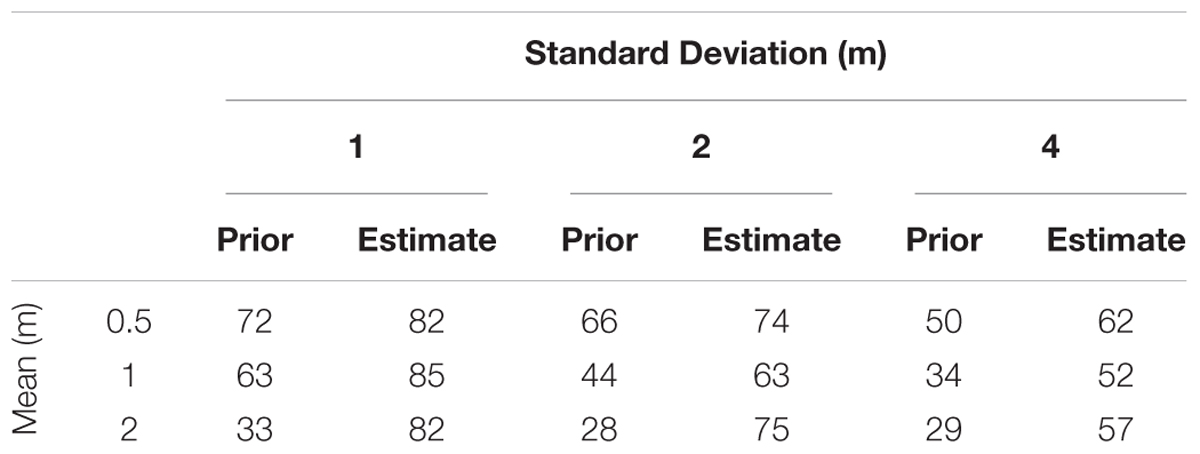
Table 2. True positive rate (TPR) at peak inundation.

Conclusion

We successfully implemented a new algorithm to improve topography information in a floodplain by exploiting indirect information of ground elevations from observed flood extents. In synthetic tests, the algorithm reduced the bias, standard deviation of errors and RMSE. Our primary motivation to produce better topography was to obtain DEMs that are more suitable for flood inundation simulations. The improved DEM we obtained from this algorithm also predicted flood inundation much better than the prior. We implemented the algorithm for nine different cases with varying mean and standard deviation of errors, and obtained similar trends in the reduction of bias and standard deviation of errors. In fact, the magnitude and percentage reduction in bias increases in cases with higher errors. The results from the synthetic tests show potential, and we believe that the method could be used to improve DEM accuracy. For example, SRTM DEM could be used as prior, along with flood inundation observations obtained from Landsat or radar to obtain a DEM with better elevation accuracy.

Digital elevation models are the primary source of topographic information, and accurate DEMs are hard to obtain in the developing world. Globally available open-source products are easy to obtain, but are not accurate. Hence, they not suitable for flood inundation modeling (Fernández et al., 2016). It is not always physically or financially feasible to obtain lidar DEMs in data-poor regions. An algorithm to improve already available DEMs is one way we can study these regions, and make better predictions. This study has produced promising results, and we believe this algorithm can be applied to real world cases to improve floodplain topography. This will provide us with higher accuracy DEMs in data-poor floodplains which are suitable for flood inundation simulations.

Author Contributions

All authors designed the model and the computational framework and wrote the manuscript. AS performed the analysis and interpretation of data.

Funding

This work was funded by NASA Headquarters under the NASA Earth and Space Science Fellowship Program (Grant 80NSSC17K0322).

Conflict of Interest Statement

The authors declare that the research was conducted in the absence of any commercial or financial relationships that could be construed as a potential conflict of interest.

The handling Editor declared a past co-authorship with one of the authors MD.

References

Bates, P. D., and De Roo, A. P. J. (2000). A simple raster-based model for flood inundation simulation. J. Hydrol. 236, 54–77. doi: 10.1016/S0022-1694(00)00278-X

CrossRef Full Text | Google Scholar

Bates, P. D., Horritt, M. S., and Fewtrell, T. J. (2010). A simple inertial formulation of the shallow water equations for efficient two-dimensional flood inundation modelling. J. Hydrol. 387, 33–45. doi: 10.1016/j.jhydrol.2010.03.027

CrossRef Full Text | Google Scholar

Carlisle, B. H. (2005). Modelling the spatial distribution of DEM error. Trans. GIS 9, 521–540. doi: 10.1111/j.1467-9671.2005.00233.x

CrossRef Full Text | Google Scholar

Cohen, S., Brakenridge, G. R., Kettner, A., Bates, B., Nelson, J., McDonald, R., et al. (2018). Estimating floodwater depths from flood inundation maps and topography. J. Am. Water Resour. Assoc. 54, 847–858. doi: 10.1111/1752-1688.12609

CrossRef Full Text | Google Scholar

Durand, M., Andreadis, K. M., Alsdorf, D. E., Lettenmaier, D. P., Moller, D., and Wilson, M. (2008). Estimation of bathymetric depth and slope from data assimilation of swath altimetry into a hydrodynamic model. Geophys. Res. Lett. 35:L20401. doi: 10.1029/2008GL034150

CrossRef Full Text | Google Scholar

Eineder, M., Fritz, T., Abdel Jaber, W., Rossi, C., and Breit, H. (2012). “Decadal Earth topography dynamics measured with TanDEM-X and SRTM,” in International Geoscience and Remote Sensing Symposium (IGARSS), (Munich), doi: 10.1109/IGARSS.2012.6351130

CrossRef Full Text | Google Scholar

Erdoǧan, S. (2010). Modelling the spatial distribution of DEM error with geographically weighted regression: an experimental study. Comput. Geosci. 36, 34–43. doi: 10.1016/j.cageo.2009.06.005

CrossRef Full Text | Google Scholar

Fernández, A., Najafi, M. R., Durand, M., Mark, B. G., Moritz, M., Jung, H. C., et al. (2016). Testing the skill of numerical hydraulic modeling to simulate spatiotemporal flooding patterns in the Logone floodplain, Cameroon. J. Hydrol. 539, 265–280. doi: 10.1016/j.jhydrol.2016.05.026

CrossRef Full Text | Google Scholar

Fisher, P. (1998). Improved modeling of elevation error with geostatistics. Geoinformatica 2, 215–233. doi: 10.1023/A:1009717704255

CrossRef Full Text | Google Scholar

Hostache, R., Lai, X., Monnier, J., and Puech, C. (2010). Assimilation of spatially distributed water levels into a shallow-water flood model. Part II: use of a remote sensing image of mosel river. J. Hydrol. 390, 257–268. doi: 10.1016/j.jhydrol.2010.07.003

CrossRef Full Text | Google Scholar

Hunter, G. J., and Goodchild, M. F. (1997). Modeling the uncertainty of slope and aspect estimates derived from spatial databases. Geogr. Anal. 29, 35–49. doi: 10.1111/j.1538-4632.1997.tb00944.x

CrossRef Full Text | Google Scholar

Krieger, G., Moreira, A., Fiedler, H., Hajnsek, I., Zink, M., and Werner, M. (2006). “TanDEM-X: Mission concept, product definition and performance prediction,” in Proceedings European Conference on Synthetic Aperture Radar (EUSAR), (Dresden).

Google Scholar

Kyriakidis, P. C., Shortridge, A. M., and Goodchild, M. F. (1999). Geostatistics for conflation and accuracy assessment of digital elevation models. Int. J. Geogr. Inf. Sci. 13, 677–707. doi: 10.1080/136588199241067

CrossRef Full Text | Google Scholar

Lai, X., and Monnier, J. (2009). Assimilation of spatially distributed water levels into a shallow-water flood model. Part I: mathematical method and test case. J. Hydrol. 377, 1–11. doi: 10.1016/j.jhydrol.2009.07.058

CrossRef Full Text | Google Scholar

Margulis, S. A., Girotto, M., Cortés, G., and Durand, M. (2015). A particle batch smoother approach to snow water equivalent estimation. J. Hydrometeorol. 16, 1752–1772. doi: 10.1175/JHM-D-14-0177.1

CrossRef Full Text | Google Scholar

Mason, D. C., Trigg, M., Garcia-Pintado, J., Cloke, H. L., Neal, J. C., and Bates, P. D. (2016). Improving the TanDEM-X digital elevation model for flood modelling using flood extents from synthetic aperture radar images. Remote Sens. Environ. 173, 15–28. doi: 10.1016/j.rse.2015.11.018

CrossRef Full Text | Google Scholar

Matgen, P., Schumann, G., Henry, J. B., Hoffmann, L., and Pfister, L. (2007). Integration of SAR-derived river inundation areas, high-precision topographic data and a river flow model toward near real-time flood management. Int. J. Appl. Earth Obs. Geoinf. 9, 247–263. doi: 10.1016/j.jag.2006.03.003

CrossRef Full Text | Google Scholar

Monnier, J., Couderc, F., Dartus, D., Larnier, K., Madec, R., and Vila, J. P. (2016). Inverse algorithms for 2D shallow water equations in presence of wet dry fronts: application to flood plain dynamics. Adv. Water Resour. 97, 11–24. doi: 10.1016/j.advwatres.2016.07.005

CrossRef Full Text | Google Scholar

Rodriguez, E., Morris, C., and Belz, J. (2006). An assessment of the SRTM topographic products. Photogramm. Eng. Remote Sensing 72, 249–260.

Google Scholar

Sampson, C. C., Smith, A. M., Bates, P. D., Neal, J. C., and Trigg, M. A. (2016). Perspectives on open access high resolution digital elevation models to produce global flood hazard layers. Front. Earth Sci. 3:85. doi: 10.3389/feart.2015.00085

CrossRef Full Text | Google Scholar

Sanders, B. F. (2007). Evaluation of on-line DEMs for flood inundation modeling. Adv. Water Resour. 30, 1831–1843. doi: 10.1016/j.advwatres.2007.02.005

CrossRef Full Text | Google Scholar

Schumann, G. J. P., Bates, P. D., Neal, J. C., and Andreadis, K. M. (2014). Technology: fight floods on a global scale. Nature 507:169. doi: 10.1038/507169e

PubMed Abstract | CrossRef Full Text | Google Scholar

Schumann, G. J.-P., and Domeneghetti, A. (2016). Exploiting the proliferation of current and future satellite observations of rivers. Hydrol. Process. 30, 2891–2896. doi: 10.1002/hyp.10825

CrossRef Full Text | Google Scholar

Yamazaki, D., Baugh, C. A., Bates, P. D., Kanae, S., Alsdorf, D. E., and Oki, T. (2012). Adjustment of a spaceborne DEM for use in floodplain hydrodynamic modeling. J. Hydrol. 436–437, 81–91. doi: 10.1016/j.jhydrol.2012.02.045

CrossRef Full Text | Google Scholar

Yamazaki, D., Ikeshima, D., Tawatari, R., Yamaguchi, T., O’Loughlin, F., Neal, J. C., et al. (2017). A high-accuracy map of global terrain elevations. Geophys. Res. Lett. 44, 5844–5853. doi: 10.1002/2017GL072874

CrossRef Full Text | Google Scholar

Yan, K., Di Baldassarre, G., Solomatine, D. P., and Schumann, G. J. P. (2015). A review of low-cost space-borne data for flood modelling: topography, flood extent and water level. Hydrol. Process. 29, 3368–3387. doi: 10.1002/hyp.10449

CrossRef Full Text | Google Scholar

Yeh, W. W.-G. (1986). Review of parameter identification procedures in groundwater hydrology: The inverse problem. Water Resour. Res. 22, 95–108. doi: 10.1029/WR022i002p00095

CrossRef Full Text | Google Scholar