Smart Speed Imaging in Digital Image Correlation: Application to Seismotectonic Scale Modeling

1. Introduction

During earthquakes elastic stress and strain is suddenly released in the lithosphere, causing abrupt relative motion of two adjacent crustal blocks. Earthquakes are usually bound spatially to a discontinuity (e.g., fault, or fault zone) and often occur in a quasiperiodic manner over geological timescales (ka to Ma) (Hyndman and Hyndman, 2016). According to the elastic rebound theory, each earthquake is preceeded by a period of seismic quiescence, followed by the earthquake and associated postseismic deformation (Reid, 1910). This cyclic behavior is termed “seismic cycle” and is the basis for assessing the geologic evolution of a seismogenic fault and the seismic hazard associated with it (Scholz, 2010). It is characterized by strongly contrasting strain rates in the interseismic and coseismic phase. During the interseismic period the system is frictionally locked, loaded at low rates (mm/a) and elastic strain gradually builds up (Tse et al., 1985; Schurr et al., 2014). In some cases the fault is not completely locked and shows slow creep deformation, e.g., in the form of slow slip events (Ide et al., 2007; Bürgmann, 2018). If the accumulated strain leads to stresses that exceed the frictional strength of the locked patch, a slip event nucleates and results in an earthquake with slip velocities in the range of m/s.

Although the recurrence behavior of earthquakes on a single fault is quasiperiodic, under the assumption of constant loading rates and frictional parameters, it is not possible to predict the onset of seismic slip (Ben-Zion et al., 2003). Therefore, numerical simulations and physical experiments have been designed to model fault slip and the seismic cycle (Rosenau et al., 2017). Because of the multiscale nature of fault slip, many numerical simulations are limited to either short (e.g., rupture models) (Heinecke et al., 2014) or long timescales (e.g., geodynamic models) (Dinther et al., 2013). Only few numerical techniques allow the combination of short term and long term processes, and frequently the parametrization and implementation of the non-linear, multiscale interactions between the long and short timescales remains difficult (Avouac, 2015). Seismotectonic analog experiments allow to address the multiscale nature of slip on a laboratory scale and may provide additional insight into the deformation over multiple seismic cycles (Rosenau et al., 2017). Even though the analog experiments are strong simplifications of a seismogenic fault system, they inherently show stick-slip dynamics without the need of a complex integration scheme (Caruso et al., 2007; Marković and Gros, 2014).

The strong variation of slip rate during the interseismic and coseismic period is the main challenge for monitoring the physical experiment (Figure 1). To capture the full rupture and associated coseismic deformation, the camera has to run at high image rates. Usually, there are two modes of recording a slip event. Either the camera is always running at high frame rate, and the images are only stored after a trigger is send (typical for very high speed cameras F > 1kHz). This only captures one rupture at a time, and does not provide constant monitoring over the complete seismic cycle. The other possibility is to monitor at a constant frame rate and storing all the images. This provides a constant monitoring but requires large amounts of data to be stored during an experiment which either is limited by the total amount of storage available (e.g., on the harddrive) or by the maximum rate of data transfer (e.g., memory to harddrive). Although, some cameras allow a change in recording frequency during the recording, this is not possible for experiments with non-predictable and very short events (t_d < 3s), because the event is over before the frame rate can be adjusted manually.

FIGURE 1

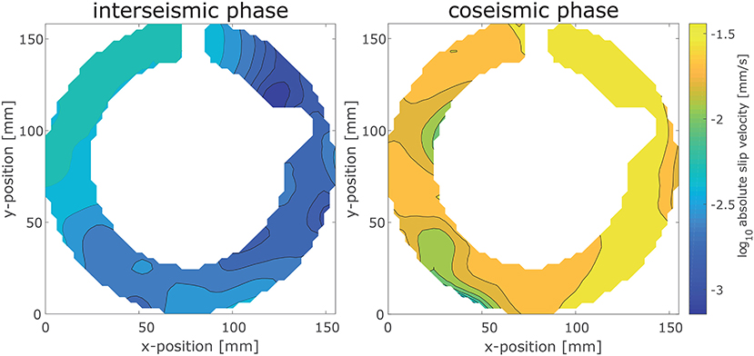
Figure 1. Comparison of the slip velocity in the experimental setup during the interseismic (Left) and coseismic (Right) phase. The slip velocity during an event is almost 2 orders of magnitude higher than during the interseismic phase. The colorbar is valid for both plots.

The images taken during the experiment are then processed using digital image correlation which yields the displacement field of slip on the fault. Ideally, the experiments run for a long time, to supply a large number of seismic cycles under constant experimental conditions (N > 100), for a good statistical analysis. For the presented experiments, this means a very large number of images which have to be processed which takes a long time, even when using a longer time interval and fewer images, the slip events have to be selected and individually processed.

In this study we present a new technique which allows for continuous monitoring of seismic cycles in seismotectonic scale models and analog earthquake models. The setup provides in-situ of shear stress and dilation, under variable normal stresses and loading rates, combined with a dynamic imaging technique. The measurements coming from the setup are used to trigger a switch from low to high framerates, resulting in drastically reduced amounts of data generated by the monitoring system. Moreover, the trigger system is combined with a buffer of images, supplying a temporary storage, which is used to fetch a certain amount of older images previously taken. Internally in the camera system this is implemented similar to a first-in-first-out (FIFO) but with access to the contained elements. This allows to increase the total duration of an experiment, while maintaining the ability to monitor the onset of seismic slip and the coseismic deformation at high rates.

2. Experimental Setup and Methods

To produce regular stick-slip oscillations we utilize a rotary shear apparatus (ring-shear-tester), normally used for testing granular material properties (details in Schulze, 1994; ASTM International, 2016). Two different sets of experiments are used to show the performance and suitability of the triggering mechanism. The first configuration uses the ring-shear-tester in standard configuration, filled with rice which produces strong stick-slip events that are very regular (Rosenau et al., 2009). The second configuration is a rotary version of typical block sliders, featuring an annular gelatine block that slides on glass beads. The individual experiments are monitored using a camera system that is connected with the triggering system. A complete overview of all components used and how they are connected is provided by Figure 2 and Table 1.

FIGURE 2

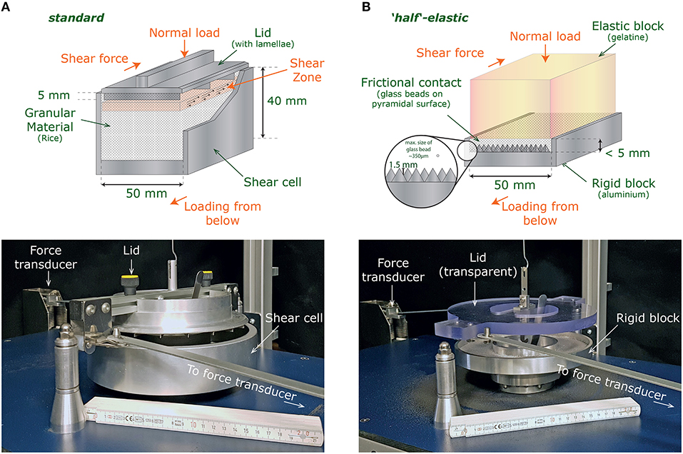
Figure 2. Schematics and photographs of the setups on which the trigger algorithm is tested. (A) Standard configuration with cell and high stiffness. The basal cell is rotated while the lid is stationary and used to measure the shear force. According to Schulze (1994), a shear zone forms below the lamellae within the glass beads. (B) Half-elastic configuration with a rigid base block, an elastic gelatine ring with a layer of glass beads in between. Here the shear zone originates at the contact between gelatine and glass beads.

TABLE 1

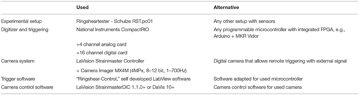
Table 1. Components and input parameters needed for the triggering algorithm.

2.1. Experimental Setup

A Schulze ring-shear-tester (Schulze, 1994) is used as a basis for the experimental setups (Figure 2). This machine measures shear forces during rotary shear of a granular material (e.g., sand, glass beads; see also Panien et al., 2006; Klinkmüller et al., 2016; Ritter et al., 2016). During the experiment, it is possible to vary normal load and shear velocity. The ring-shear-tester uses a cantilever in combination with a motorized weight to hold a constant normal stress. The cantilever pulls the lid downwards onto the sample inducing normal stresses of 0.5–20 kPa. A digitally controlled motor rotates the shear cell at velocities V_L in the order of 10⁻⁴ to 10⁻¹ mm/s. For the experiments in this study, we use velocities from 8.3 × 10⁻⁴ to 1.6 × 10⁻² mm/s and normal stresses between 5 and 20 kPa. A twin beam system coupled to inductive displacement transducers measures the shear forces during the experiment at a frequency of up to F = 50kHz. The stiffness of the complete experimental setup is k = 1, 354Nm (Schulze, 1994).

2.1.1. Standard Configuration

We use the ring-shear-tester RSTpc.01 in standard configuration with the annular shear cell that has an inner sample diameter of 10 cm, an outer diameter of 20 cm, and a thickness of 4 cm (Figure 2A, cell type (Schulze, 1994). The aluminum shear cell has a high friction bottom, defined by evenly spaced grooves. As granular material we use a typical “thai” rice (sample “RI-1,” Table 2), which has previously been found to show ideal stick-slip characteristics that are needed to test the triggering algorithm (Rosenau et al., 2009, 2017). A solid, aluminum lid, with lamellae providing a high friction interface, is placed on top of the rice. The upper surface of the lid is covered with a white-on-black random pattern of dots, which is ideal for the later digital image correlation (section 2.2). Because the lid is rigid, only the bulk deformation of the rice is recovered by monitoring the surface. We use this setup to illustrate the performance of the trigger system, because it produces almost perfect stick-slip cycles with a very long interevent phase in comparison to the slip events.

TABLE 2

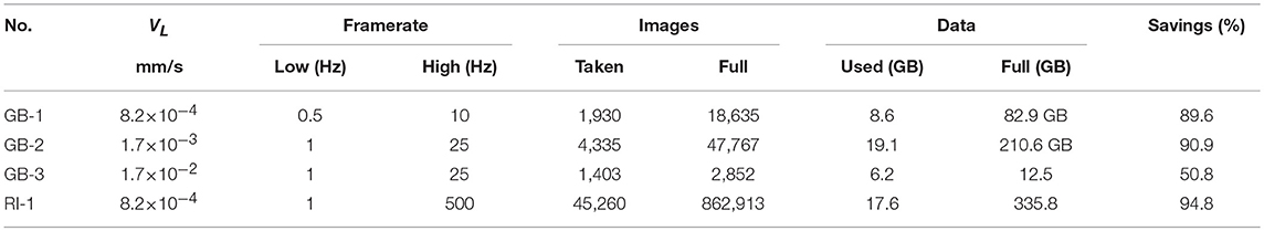
Table 2. Recording rates and data savings per experiment.

2.1.2. Block Slider Configuration

For the block slider model, we use a thinner shear cell (Figure 2B, gelatin not included in the image), which is completely filled with glass beads (samples “GB-1” to “GB-3,” Table 2). On top of the glass beads an annular ring of gelatin provides elastic boundary conditions and acts as a lid. The gelatine is 25w% pig skin gelatin (Italgelatin, see also Di Giuseppe et al., 2009) which has a Young's Modulus E ≈ 150…200kPa and is transparent. On top of the gelatin a polycarbonate lid provides a stiff connection to the force transducers and provides the possibility to observe the glass bead layer from the top.

The shear cell has a bottom that is covered with a pattern of 2 × 2 × 2 mm pyramids which provides a very high basal friction along the bottom of the glass beads. The glass beads are filled into the shear cell according to the procedure given by Klinkmüller et al. (2016). The glass beads are spherical with an average diameter of 300–400 μm and a coefficient of friction μ of 0.3 to 0.5. For better detection with the image correlation algorithm 10% of glass beads are colored with diluted black acrylic paint. We use the same mixture of glass beads throughout all experiments.

2.2. Monitoring System

Over the whole experimental duration the top surface of the lid (standard configuration), or glass bead layer (block slider configuration), is monitored with a 4 MPx and 8–12 bit CMOS¹ camera (top left in Figure 3, Imager MX4M, by LaVision). Depending on the speed of the observed process the frame rate is adaptable to values between 0.5 and >500 Hz. The observed surface is illuminated by a continuous LED light (100 kHz, 100% duty cycle) to prevent changing brightness because of the 50 Hz power grid frequency. The images are calibrated with a rectangular pattern of dots. This calculates the spatial scale per pixel and adjusts for lens distortion.

FIGURE 3

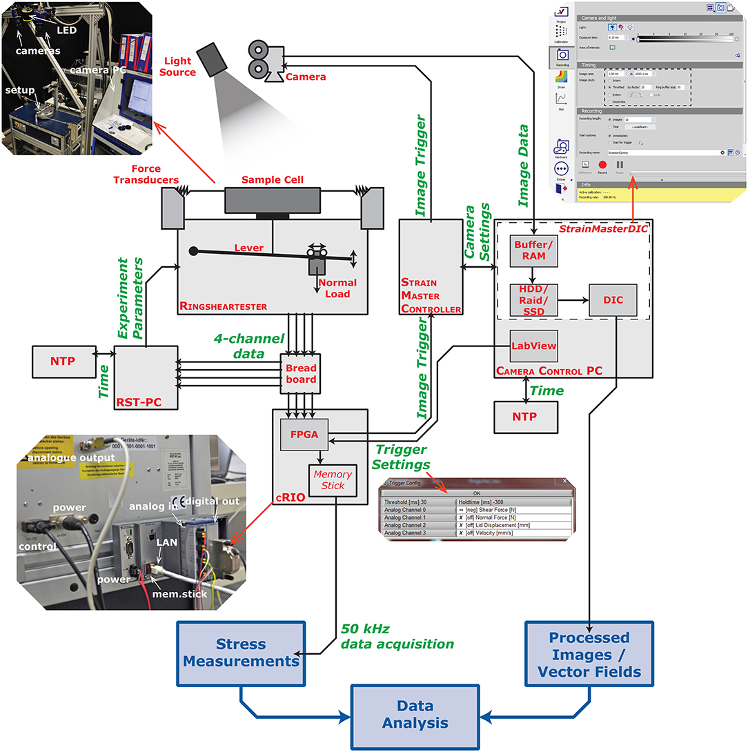
Figure 3. Schematic diagram showing the setup and the connections to the monitoring system. The ring-shear-tester is controlled by a computer (RST-PC), which sets the parameters for the experiment (e.g., shear velocity, normal stress). The CompactRIO (cRIO) is connected to the output channels and provides the triggering and recording on all four channels (F_shear, F_normal, ΔH, V_L). A second computer (Camera Control PC) is connected to the camera system which consists of a controller (StrainMaster Controller) and a software (StrainMasterDIC by LaVision). It supplies the settings for the camera (recording rate, exposure time,…) and stores the incoming image data for digital image correlation (DIC). All components are also listed in Table 1.

In our study, each acquired image has a bit depth of 8 bit which gives 265 grayscale values. In combination with a spatial resolution of 2,048 × 2,048px this results in a file size of ≈ 8 MB per image. The images are processed using the built-in digital image processing algorithm by LaVision StrainMasterDIC (top right in Figure 3). It utilizes affine transformation to match patterns at equally spaced interrogation points (step width: 8 px) between two successive images (Bouguet, 2001; Fleet and Weiss, 2005). At each point, a subset of 31 pixels is matched using the least squares matching algorithm. The algorithm gives back the displacement in the form of a 2D vector at each interrogation point. This results in a high resolution displacement field over the whole analyzed domain.

To get an appropriate catalog size, the experiments run over at least 1 h. Usually, the camera takes a continuous time series of images at a fixed frequency, e.g., 10 Hz. Due to the nature of the modeled system, the deformation during the interseismic phase of a stick-slip cycle is very low. Previously, the acquisition rate was a tradeoff, between the amount of storage available, and the speed of the process. As an example, 1 h of continuous measurement at 10 Hz covers 60–70 seismic cycles and uses approximately 288 GB of storage. For this study, we developed a triggering system that uses the shear stress measurements from the ring-shear tester to trigger a change in camera frequency from 0.5 to 1 Hz during the interseismic phase, to 10–25 Hz in the coseismic phase.

The trigger system consists of an embedded controller (center in Figure 3, National Instruments, CompactRIO) that is connected to the four channel analog output of the ring-shear tester and the trigger input of the camera system. The controller records the data with a frequency of 50 kHz which is downsampled to the requested recording frequency depending on what the user wants to record. The trigger algorithm independently utilizes the incoming 50 kHz stream and uses every 50th value to calculate the trigger level. Higher rates are theoretically possible with a more powerful logical processor (field-programmable gate array, FPGA) and digitizer (analog digital converter, ADC). Additionally, the algorithm is very simple and thus also able to run on less powerful, cheaper hardware, such as e.g., an Arduino MKR Vidor, although at a reduced rate.

2.3. Trigger Algorithm

The trigger algorithm consists of a set of conditions T = {T₁, T₂, T₃, T₄, T₅} which are logically combined to determine the output of a trigger signal T_a (Figure 4). The algorithm uses any provided input signal x and detects changes in x by comparing two differences Δ_short and Δ_long over two time intervals. These two differences are the basis for the detection and are defined as follows:

$\begin{array}{rc}{t}_{short}=\left[t_{-1},t_0\right]& (1)\end{array}$

t_short is a small time interval between the current value at t₀ and the previous value at t₋₁ which leads to:

$\begin{array}{rc}{\Delta }_{short}=x_{t_0}-x_{t_{-1}}& (2)\end{array}$

And the long time interval t_long is defined by:

$\begin{array}{rc}{t}_{long}=\left[t_w\dots t_{-1}\right]& (3)\end{array}$

This is the time between the previous value t₋₁ and a value at a defined time the past t_w, leading to:

$\begin{array}{rc}{\Delta }_{long}=x_{t_{-1}}-x_{t_w}& (4)\end{array}$

The moving window size t_w can be chosen by the user to adjust the sensitivity of the trigger algorithm. It mainly decides the time scale over which the change is going to occur. For example, if the targeted process happens over a time scale of 100 ms then the window size should be t_w ≤ 100ms. The two differences show a different reaction to transients (Figure 4A). The long term difference is slower to react, but shows a larger amplitude, whereas the short term difference is quicker but with a much smaller amplitude.

FIGURE 4

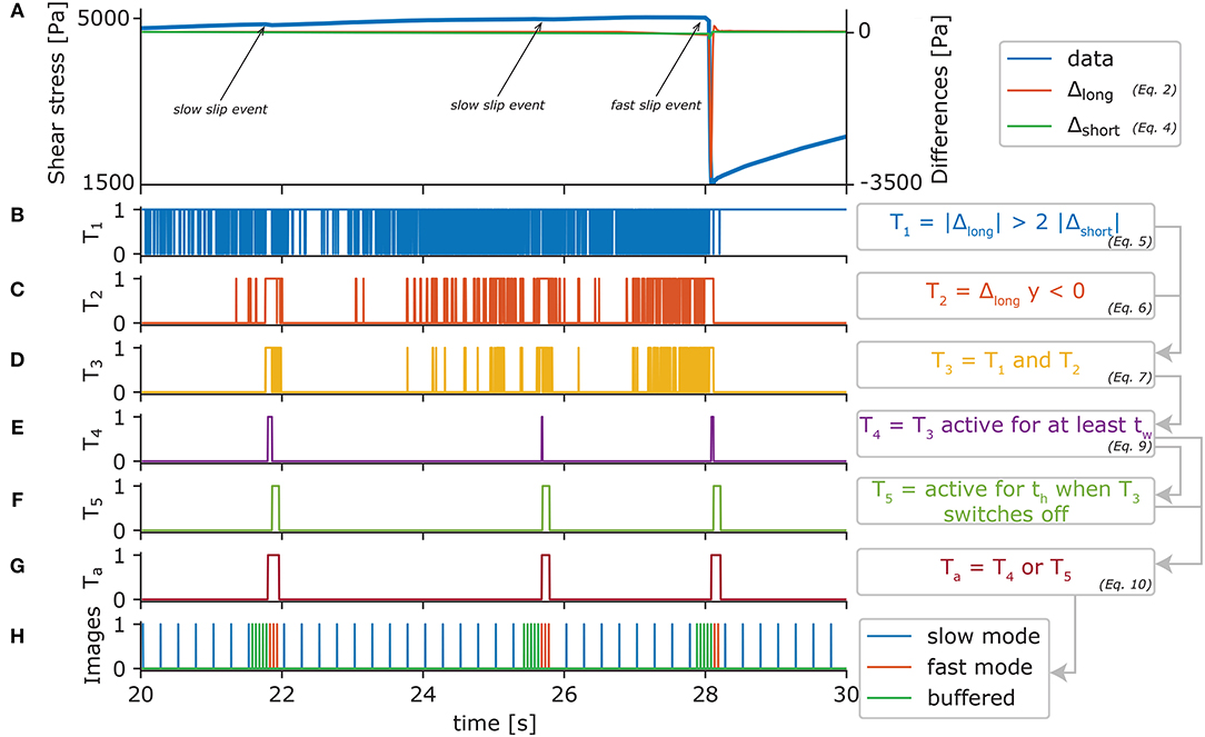
Figure 4. Behavior of the trigger algorithm during an experiment. Input parameters are: t_w = 30ms, t_h = 100ms, polarity is negative, F_high = 20Hz, n = 5, i = 5. (A) Typical shear curve of an experiment. The data contains very fast slip events and slower slip events. The latter are very difficult to detect by eye. (B–G) Individual results of the trigger conditions, with successively increasing accuracy. (H) Images taken during the experiment, distinguished by low, fast, and buffer acquisition.

To detect changes in the signal, we introduce the first condition T₁ which is true when the long term difference Δ_long is twice the amplitude of the short term difference Δ_short (Figure 4B):

$\begin{array}{rc}{T}_1({\Delta }_{long},{\Delta }_{short}):=\left\{\begin{array}{ccc}1& if& \left|{\Delta }_{long}\right|>2\left|{\Delta }_{short}\right|\\ 0& if& \left|{\Delta }_{long}\right|\le 2\left|{\Delta }_{short}\right|\end{array}\right\}& (5)\end{array}$

The factor of two reduces the influence of noise on T₁. To keep the algorithm simple and easy to predict, the factor is predefined and not changeable by the user.

Because T₁ reacts on any change, negative and positive, a second condition T₂ is used to be able to switch the polarity of the trigger (Figure 4C). The user is able to select the polarity on which the trigger should detect. In our case the input signal for the trigger algorithm is the measured shear stress. During a slip event the shear stress decreases and therefore both differences show a negative polarity. As a result, in our case T₂ is true when Δ_long is negative:

$\begin{array}{rc}{T}_2({\Delta }_{long}):=\left\{\begin{array}{ccc}1& if& {\Delta }_{long}<0\\ 0& if& {\Delta }_{long}\ge 0\end{array}\right\}& (6)\end{array}$

Equations (5) and (6) are used to determine a third condition T₃, which is true when both other conditions are true:

$\begin{array}{rc}{T}_3=T_1\wedge T_2& (7)\end{array}$

Although T₁ includes a noise reducing factor of two, T₃ is sometimes true for a few milliseconds and then deactivates again (Figure 4D). For a real slip event the conditions are met over a longer period of time, without switching off in between. As a consequence, the next trigger condition T₄ is set to true, when T₃ has been active for at least the long window size t_w (Figure 4E). This is facilitated with a simple counting variable k that is incremented when T₃ is true and set to zero when T₃ is false:

$\begin{array}{rc}k:=\left\{\begin{array}{ccc}k+1& if& T_3=1\\ 0& if& T_3=0\end{array}\right\}& (8)\end{array}$

As a result T₄ is defined by:

$\begin{array}{rc}{T}_4:=\left\{\begin{array}{ccc}1& if& k\ge t_w\\ 0& if& k<t_w\end{array}\right\}& (9)\end{array}$

To capture processes happening after a slip event, e.g., afterslip, we implemented an optional hold time t_h which defines for how long the trigger should stay active after T₄ switches back to off. This is also facilitated with an internal clock type variable that defines the trigger condition T₅ (Figure 4F). As a result, the final trigger activity that is send to the camera system T_a is a logical OR connection of T₄ and T₅, where T₄ is a combination of all previously defined conditions and T₅ only depends on the hold time t_h (Figure 4G):

$\begin{array}{rc}{T}_a=T_4\vee T_5& (10)\end{array}$

As Figures 4B–G shows, the combination of the individual trigger conditions leads to an increasingly precise detection of transients. It also detects transients which are not easily observed by the naked eye, such as the slow slip events marked in Figure 4A.

2.4. Implementation in LaVision StrainMasterDIC

Our trigger system has been integrated into the image analysis software suites StrainMasterDIC and DaVis 10 by LaVision, as an additional method of changing the framerate via an external trigger signal. The microcontroller that calculates the final trigger activity T_a gives out a 5V TTL (transistor-transistor logic) signal that is interpreted by the imaging software to trigger the cameras. The signal is in low state (0 V) when T_a = 1 and in high state (5 V) when T_a = 0. It is transferred over 50Ω coaxial cables to the programmable timing unit (LaVision Strainmaster Controller) of the camera system which then triggers the cameras.

Inherently, the trigger system is only activated when a slip event is already happening (Figure 4). Therefore, it is combined with a buffer of images (FIFO) on the memory of the computer (RAM) which is constantly filled with images from the camera at high-speed frequency F_high. The size of the buffer can be set in the software. For this study it is set to be the number of high-speed images between two subsequent low-speed images, e.g., if F_low = 1Hz and F_high = 25Hz, then the number of images in the buffer i = 25. The two different acquisition frequencies are realized by giving the high speed frequency F_high and a division factor n which slows down the acquisition when no slip event is happening. When the trigger is off (T_a = 0), the system only selects each nth image that comes out of the image buffer to be saved. As soon as the trigger is on (T_a = 1), all images in the buffer are fetched and marked for saving. Then it continues recording at high speed until the trigger switches back to off. Figure 4H shows the sequence of images recorded and whether they are taken in slow mode, fast mode, or loaded from the buffer.

3. Results

3.1. Slip Events in the Different Configurations

Both configurations show quasiperiodic stick-slip oscillations of varying amplitude and recurrence (Figure 5A). The shear force in all experiments oscillates in a sawtooth shaped pattern analogs to the shear force along a seismogenic fault. This is characteristic for sheared granular shear materials (e.g., Losert et al., 2000). Here we only give a brief overview of some of their characteristics in our setup, to illustrate the application of the trigger system.

FIGURE 5

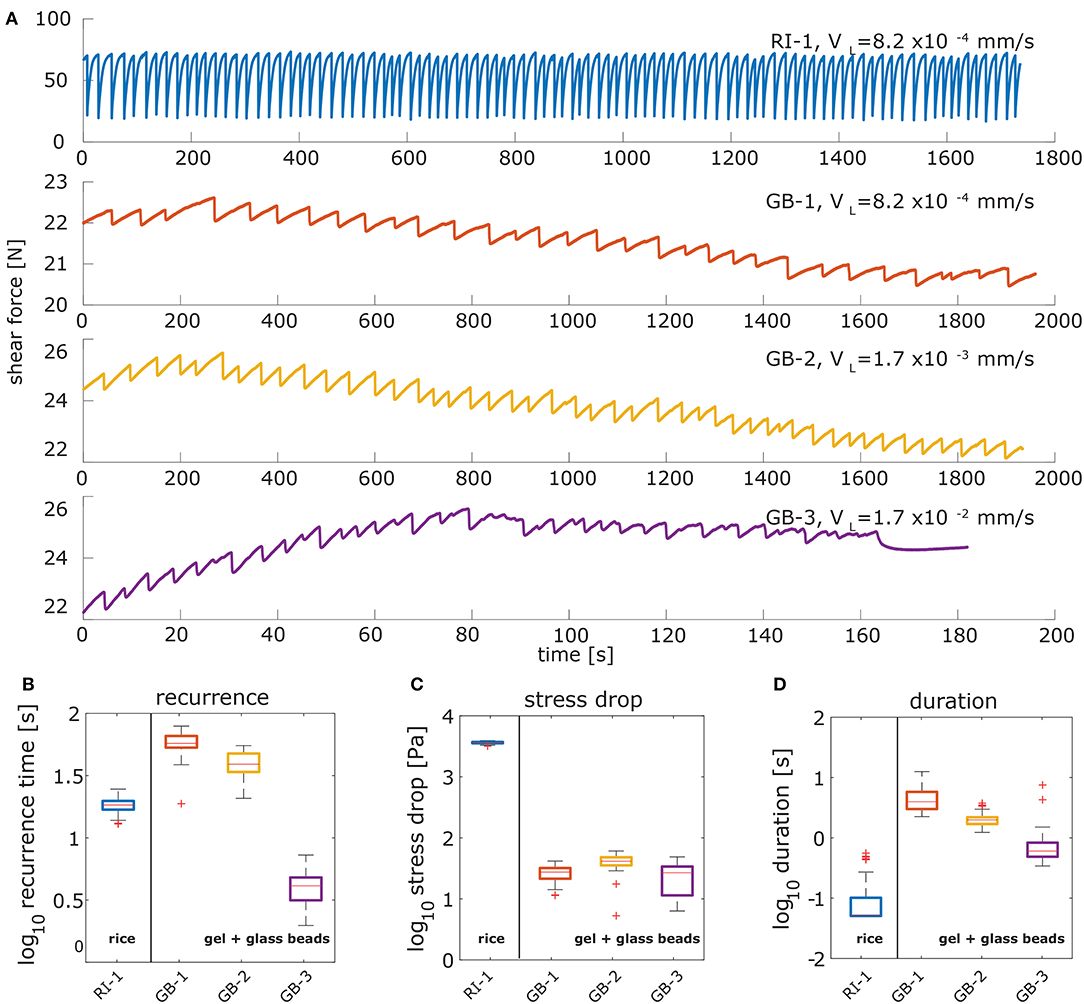
Figure 5. Shear force curves and characteristic parameters derived from the stress measurements. (A) Shear force measurements during the experiments with a characteristic saw-tooth shape. The y-axis is shear force in Newton and the x-axis is time in seconds for all experiments. (B) The realized recurrence times cover two orders of magnitude and are similar for both setups. For higher shear rates the recurrence time is significantly reduced, which is in accordance with the rate-and-state-dependent friction. (C) Stress drops cover the same range for the block slider configuration and is much higher for the standard configuration. This results mostly from the stiffness of the setup, which is several orders of magnitude higher in the standard configuration. (D) The duration of the events decreases with increasing shear rate. The detected durations of the rice stick-slips are very low and truncated at 0.1 s.

The experiment in standard configuration (RI-1, blue color) was carried out at a loading rate of $V_L=8.2\times 10^{-4}$ mm/s and a normal stress of 5 kPa. The strength of the rice grains is relatively high and reaches values above the normal stress several times. The recurrence time t_rec is very regular and is 18.3 ± 2.3s (Figure 5B). The stress drops Δτ = 3, 650 ± 150 Pa, are two orders of magnitude higher that for the block slider configuration (Figure 5C).The duration of a slip event in rice is around 0.1 s (Figure 5D). The ratio between recurrence and duration is very high ($\frac{t_{rec}}{t_{dur}}\approx$360), and as a result the potential for saving image data is very high.

In the block slider configuration three different shear rates are realized, which are in the range of the targeted values for the application of the trigger setup (GB-1, -2, and -3 in Figure 5A). Shear rates range from 8.2 × 10⁻⁴ to 1.7 × 10⁻² at normal stresses of 5 kPa. The recurrence time nonlinearly decreases with increasing shear rate, which is an expected behavior for this rate-and-state-dependent material (Figure 5B). At the highest realized shear rate the recurrence time is reduced by one order of magnitude from around 60 s down to 4 s. This is due to the occurrence of some smaller precursory events, also reflected in the lower tail of the stress drop distribution. The slip events in the block slider configuration are of much lower magnitude than in standard configuration with median stress drop ranging from 27 ± 8 to 41 ± 14 Pa (Figure 5C). Furthermore, they are less regular and have a less homogenous magnitude-size distribution, log-normal instead of normal, especially at the highest shear rate the events cover a broad range of stress drops. The duration of slip in the block slider is also decreasing with increasing shear rate and ranges between 0.6 ± 0.6 and 4 ± 2 s. The resulting ratio between duration and recurrence is in the range of 14–20 for the two lower shear rates and 7 for the higher shear rate. This ratio is not as high as for rice but because the recurrence behavior is less regular a manual trigger switch is not feasible.

3.2. Trigger Algorithm

The amount of data saved during the image acquisition ranges between ≈50 and 95% (Table 2). Experiments which show a very regular and ideal stick-slip behavior show the highest amount of data saved (GB-1, GB-2, and RI-1). If the slip events are less regular, or are dissected by transient slip events that are much slower than the actual event, the algorithm triggers more often, and therefore more data is produced (GB-3). Nevertheless, the trigger system is able to save more than 50% of data. Slight refinements to the detection thresholds or frame rates can help to push this limitation a bit further. Correctly adjusting the window size to the faster events lowers the amount of false detections and a higher “slow” framerate helps to cover the slower events with more accuracy.

The trigger algorithm also decreases the average framerate over the duration of the whole experiment, e.g., ≈26Hz for RI-1. This limits the average amount of data per second from 200 to 10 MB/s which enables the use of inexpensive single hard-drive systems instead of a raid configuration. The software does not immediately save the images onto the harddrive, but transfers the selected images into another buffer (FIFO) in the RAM that saves the images as fast as the harddrive can save them. Therefore, the incoming images are distributed over a longer period of time which reduces the storage rate needed. The delay between trigger signal and reaction of the camera system is in the order of a few μs which provides a very quick reaction to the trigger signal. If the two window sizes are well adjusted, the complete onset of the slip event and the postseismic effects are recorded at high speed, whereas the interseismic phase is covered at reduced rate. In extreme cases (full resolution and framerate) the camera used in this study produces around 1 GB/s which can be lowered to around 100 MB/s, assuming a typical reduction by 90%. Usually this system requires a multi-disk raid that can store up to 1.8 GB/s in combination with a large RAM (>128 GB) to record images over the duration of 1 h. This is not needed anymore, when using the provided trigger system.

4. Discussion and Conclusion

4.1. Time Synchronization

Combining experimental results from different monitoring systems requires a reliable time stamp on the images and on the signal data. To synchronize the time between multiple computers in our setup we use the network time protocol (NTP). A specialized software continuously synchronizes each computer with the two network time servers of the local area network at the institute. The network time servers synchronize with GPS signals and the software automatically calculates the delay and offset within the network. This is a standard facility that is necessary for many LAN networks and should be generally available at most universities or research institutions. If only the time synchronization with internet servers provided by the operating system is used, e.g., Windows time service, we found that the time difference between two individual computers can be up to several seconds. For seismotectonic scale models with slip events that occur on the millisecond time scale, this is not feasible. Therefore, it is advised to either use a single computer for everything, or to synchronize the time between the individual devices by using an external clock generator using a specialized software.

4.2. Digital Image Correlation

The reduction of produced images yields much faster processing times for the digital image correlation. This speeds up the typical workflow of an analog experiment. Additionally, the signal to noise ratio is improved during the interseismic time. Because the framerate is adjusted to the coseismic velocities, the interseismic deformation often is below the detection threshold of the digital image correlation algorithm, which is usually in the subpixel range. Lower framerates during the interseismic time increase the total amount of deformation recorded per image providing a much more accurate estimation of interseismic deformation, that is needed for example to calculate the interseismic locking.

4.3. Alternative Triggering Systems

4.3.1. With a Priori Data Reduction

Our trigger system serves as an a priori reduction of data. It is therefore most efficient when the observations are preceded by some sort of precursor, or if additional observations, such as the force measurements, are available. Furthermore, it relies on the temporal storage of images with dynamic access to the buffer which is not available for most systems. Some camera systems allow for post-triggering, which means that they have a static buffer which is emptied after an event has been triggered. These only support one frame rate, and the triggering process has to be fast enough, that an overflow of the buffer is prevented. The triggering can be automated with the presented setup, or manual by visual inspection of the experiment. This technique can be feasible when a reliable signal is not available and should be accompanied by a continuous monitoring at lower frequency with a second camera.

In some cases a reliable secondary signal, such as the force measurements, is not available because the setup is technically not feasible. This is the case for many analog experiments, like wedges and sandboxes. For these experiments a reliable stress measurement is geometrically hindered or the stress transmission to a sensor is limited. Such experiments can be monitored using a simultaneous strain measurement by digital image correlation. Especially when the observed deformations are too small to be visible by the naked eye, which makes the manual post-triggering impossible. The real-time strain gage also requires a buffer and a performant computer system which is able to compute a quick strain estimation from the images. If these requirements are met, the system is similar to our trigger system and can either use a velocity or acceleration threshold to trigger the high-speed acquisition of images.

4.3.2. With a Posteriori Data Reduction

If a buffer on the computer ram or camera ram is not available, e.g., for consumer grade digital cameras, the above algorithm can be used to do quick a posteriori sorting of images. During the experimental run but with some time delay. Then the images have to be transmitted to a computer during the experimental run which is also possible for many standard digital cameras where the manufacturer supplies a specialized software to remote control the camera via USB. Using a script, or the PC component of the embedded microcontroller (“RealTime” for the CompactRIO), the trigger is used to delete the unnecessary images during the interseismic phase. Alternatively, the recorded signal can be used after the experiment, to select only the images where a slip event has happened which quickens the post-experiment analysis.

4.4. Conclusions

In this study we developed a smart speed imaging technique based on an external trigger algorithm that allows for a well defined, feedback controlled change of image rate during an experiment. Our experiments verify that it is able to greatly reduce the needed amount and speed of storage. The use of a double time-frame approach is easy to adjust, while maintaining a rapid and robust response to changes in the triggering signal. The fully modular specification of the algorithm and hardware system, allows to add further input signals (e.g., acoustic emissions) without major changes. Furthermore, the lower amount of images provides a faster processing speed because less images have to be processed during digital image correlation.

In comparison with traditional approaches, such as manual triggering, the presented algorithm provides a well defined and quantifiable constraint on the detection of slip events in real-time data. It only relies on the triggered event itself and does not require any knowledge about precursory phenomena. In addition, only a few observations are needed to adjust the parameters to the optimal value.

Data Availability Statement

The datasets generated and analyzed for this study, including the scripts to generate the figures, have been published in Rudolf et al. (2019).

Author Contributions

MiR planned and performed the experiments, analyzed the data, and wrote the research paper. MaR was involved in planning the research, analyzing the results and writing. TZ, VL, TS, and HN facilitated the technical realization of the study. OO was involved in supervising the research and writing.

Funding

This research has been funded by Deutsche Forschungsgemeinschaft (DFG) through grant CRC 1114 Scaling Cascades in Complex Systems, Project B01 Fault networks and scaling properties of deformation accumulation. Additional funding was provided by the European Union Initial Training grant 674899-SUBITOP.

Conflict of Interest Statement

The outcomes of this research are partially used by LaVision Germany GmbH, who also provided access to development versions of the camera systems that they resell.

The authors declare that the research was conducted in the absence of any commercial or financial relationships that could be construed as a potential conflict of interest.

Acknowledgments

F. Neumann is acknowledged for his technical assistance in the laboratory. This study has benefitted from discussions with J. Bedford.

Footnootes

1. ^Complementary metal-oxide semiconductor.

References

ASTM International (2016). Standard Test Method for Bulk Solids Using Schulze Ring Shear Tester. West Conshohocken, PA: ASTM International. doi: 10.1520/d6773-16

CrossRef Full Text

Avouac, J.-P. (2015). From geodetic imaging of seismic and aseismic fault slip to dynamic modeling of the seismic cycle. Annu. Rev. Earth Planet. Sci. 43, 233–271. doi: 10.1146/annurev-earth-060614-105302

CrossRef Full Text | Google Scholar

Ben-Zion, Y., Eneva, M., and Liu, Y. (2003). Large earthquake cycles and intermittent criticality on heterogeneous faults due to evolving stress and seismicity. J. Geophys. Res. 108:B6. doi: 10.1029/2002JB002121

CrossRef Full Text | Google Scholar

Bouguet, J.-Y. (2001). Pyramidal Implementation of the Affine Lucas Kanade Feature Tracker Description of the Algorithm. Intel Corporation.

Bürgmann, R. (2018). The geophysics, geology and mechanics of slow fault slip. Earth Planet. Sci. Lett. 495, 112–134. doi: 10.1016/j.epsl.2018.04.062

CrossRef Full Text | Google Scholar

Caruso, F., Pluchino, A., Latora, V., Vinciguerra, S., and Rapisarda, A. (2007). Analysis of self-organized criticality in the olami-feder-christensen model and in real earthquakes. Phys. Rev. E 75:055101. doi: 10.1103/PhysRevE.75.055101

PubMed Abstract | CrossRef Full Text | Google Scholar

Di Giuseppe, E., Funiciello, F., Corbi, F., Ranalli, G., and Mojoli, G. (2009). Gelatins as rock analogs: a systematic study of their rheological and physical properties. Tectonophysics 473, 391–403. doi: 10.1016/j.tecto.2009.03.012

CrossRef Full Text | Google Scholar

Dinther, Y., Gerya, T. V., Dalguer, L. A., Mai, P. M., Morra, G., and Giardini, D. (2013). The seismic cycle at subduction thrusts: insights from seismo-thermo-mechanical models. J. Geophys. Res. 118, 6183–6202. doi: 10.1002/2013JB010380

CrossRef Full Text | Google Scholar

Fleet, D., and Weiss, Y. (2005). “Optical flow estimation,” in Handbook of Mathematical Models in Computer Vision, eds N. Paragios, Y. Chen, and O. Faugeras, O (Springer), 239–258. Available online at: http://www.cs.toronto.edu/~fleet/research/Papers/flowChapter05.pdf

Google Scholar

Heinecke, A., Breuer, A., Rettenberger, S., Bader, M., Gabriel, A. A., Pelties, C., et al. (2014). “Petascale high order dynamic rupture earthquake simulations on heterogeneous supercomputers,” in SC14: International Conference for High Performance Computing, Networking, Storage and Analysis (New Orleans, LA), 3–14. doi: 10.1109/SC.2014.6

CrossRef Full Text | Google Scholar

Hyndman, D., and Hyndman, D. (2016). Natural Hazards and Disasters. Cengage Learning. Verlag: Boston, MA.

Google Scholar

Ide, S., Beroza, G. C., Shelly, D. R., and Uchide, T. (2007). A scaling law for slow earthquakes. Nature 447, 76–79. doi: 10.1038/nature05780

PubMed Abstract | CrossRef Full Text | Google Scholar

Klinkmüller, M., Schreurs, G., Rosenau, M., and Kemnitz, H. (2016). Properties of granular analogue model materials: a community wide survey. Tectonophysics 684, 23–38. doi: 10.1016/j.tecto.2016.01.017

CrossRef Full Text | Google Scholar

Losert, W., Bocquet, L., Lubensky, T. C., and Gollub, J. P. (2000). Particle dynamics in sheared granular matter. Phys. Rev. Lett. 85, 1428–1431. doi: 10.1103/PhysRevLett.85.1428

PubMed Abstract | CrossRef Full Text | Google Scholar

Marković, D., and Gros, C. (2014). Power laws and self-organized criticality in theory and nature. Phys. Rep. 536, 41–74. doi: 10.1016/j.physrep.2013.11.002

CrossRef Full Text | Google Scholar

Panien, M., Schreurs, G., and Pfiffner, A. (2006). Mechanical behaviour of granular materials used in analogue modelling: insights from grain characterisation, ring-shear tests and analogue experiments. J. Struct. Geol. 28, 1710–1724. doi: 10.1016/j.jsg.2006.05.004

CrossRef Full Text | Google Scholar

Reid, H. (1910). The Mechanism of the Earthquake. The California earthquake of april 18, 1906: Report of the State Investigation Commission, Vol. 2. Washington, DC: Carnegie Institution of Washington.

Google Scholar

Ritter, M. C., Leever, K., Rosenau, M., and Oncken, O. (2016). Scaling the sand box - mechanical (dis-) similarities of granular materials and brittle rock. J. Geophys. Res. Solid Earth 121, 6863–6879. doi: 10.1002/2016JB012915

CrossRef Full Text | Google Scholar

Rosenau, M., Corbi, F., and Dominguez, S. (2017). Analogue earthquakes and seismic cycles: experimental modelling across timescales. Solid Earth 8, 597–635. doi: 10.5194/se-8-597-2017

CrossRef Full Text | Google Scholar

Rosenau, M., Lohrmann, J., and Oncken, O. (2009). Shocks in a box: an analogue model of subduction earthquake cycles with application to seismotectonic forearc evolution. J. Geophys. Res. 114:B1. doi: 10.1029/2008JB005665

CrossRef Full Text | Google Scholar

Rudolf, M., Rosenau, M., Ziegenhagen, T., Ludwikowski, V., Schucht, T., Nagel, H., et al. (2019). Supplement to: smart speed imaging in digital image correlation: application to seismotectonic scale modelling. GFZ Data Serv. 1–2. doi: 10.5880/GFZ.4.1.2018.002

CrossRef Full Text | Google Scholar

Scholz, C. H. (2010). Large earthquake triggering, clustering, and the synchronization of faults. Bull. Seismol. Soc. Am. 100, 901–909. doi: 10.1785/0120090309

CrossRef Full Text | Google Scholar

Schulze, D. (1994). Development and application of a novel ring shear tester. Aufbereit. Tech. 35, 524–535.

Google Scholar

Schurr, B., Asch, G., Hainzl, S., Bedford, J., Hoechner, A., Palo, M., et al. (2014). Gradual unlocking of plate boundary controlled initiation of the 2014 iquique earthquake. Nature 512, 299–302. doi: 10.1038/nature13681

PubMed Abstract | CrossRef Full Text | Google Scholar

Tse, S. T., Dmowska, R., and Rice, J. R. (1985). Stressing of locked patches along a creeping fault. Bull. Seismol. Soc. Am. 75:709.

Google Scholar