Seasonal Dynamics of Methane and Carbon Dioxide Evasion From an Open System Pingo: Lagoon Pingo, Svalbard

Introduction

It has been known for some time that the transition from the Last Glacial Maximum was characterized by rapid methane escape from source(s) either associated with or influenced by continental ice sheets in the Northern Hemisphere (Björklund, 1990; Smith et al., 2001; Weitemeyer and Buffett, 2006). More recently, great attention has been given to the potential contribution made to this flux by the destabilization of sub-ice sheet clathrate deposits, resulting in fluid discharge via vents known as “pockmarks.” These are particularly well-preserved features in the glaciomarine sediments of West Spitsbergen fjords and parts of the continental shelf (Forwick et al., 2009; Roy et al., 2015; Portnov et al., 2016). The extent to which the pockmarks remain active today is unclear, but there is well-known methane evasion associated with clathrate destabilization on the continental shelf, enhanced partly by isostatic uplift (Wallmann et al., 2018). However, only a very minor proportion of the methane released actually reaches the atmosphere due to oxidation and methanotrophy in the oxic surficial sediments and water column (Gentz et al., 2014; Hong et al., 2016; Myhre et al., 2016; Mau et al., 2017). It seems important, therefore, to consider whether active methane ventilation occurs from terrestrial sites where fluid discharges are able to by-pass deep water columns or soil (active layer) environments conducive to methane oxidation. A hitherto overlooked possibility is that isostatic rebound has uplifted pockmarks, enabling their transition from submarine into terrestrial seepages. This is made feasible by the marked effects of sea level change on the coastal environment of West Spitsbergen and other parts of the Arctic, including Greenland (e.g., Gilbert et al., 2017, 2018). Such uplifted coastal lowlands are often characterized by groundwater springs that are manifest as icings on account of their winter discharge and freezing upon emergence at the ground surface. However, in cases where the freezing starts to occur before emergence, they can be manifest as open system pingos (Yoshikawa, 1993; Yoshikawa and Harada, 1995; Liestøl, 1996).

Open system pingos in Svalbard are thought to form under three circumstances that result in groundwater freezing, expansion and thus ground-heave, producing their characteristic hill-like form (Yoshikawa, 1993; Liestøl, 1996). They include: i) the release of subglacial meltwaters via taliks beneath the temperate parts of thicker Arctic glaciers; ii) the exploitation of geological faults by groundwater (potentially from a multitude of sources), and iii) the generation of high water pressure during permafrost aggradation as a direct response to isostatic uplift (Yoshikawa and Harada, 1995). The last mechanism is of particular interest in the present study, because it best represents the processes by which uplifted pockmarks and other fluid escape features may form terrestrial methane seeps. It is also the mode of formation previously described for Lagoon Pingo by Yoshikawa and Harada (1995), where the present study was conducted. Furthermore, there are expansive marine sediment packages whose ongoing exposure following isostatic uplift in the coastal fjord valleys of West Spitsbergen is leading to permafrost aggradation (Humlum, 2005; Gilbert et al., 2017). It therefore seems intuitive to expect discontinuities, such as those formed by fluid escape via pockmarks to continue to be exploited by upwelling groundwaters during this process. This is in stark contrast to the traditional view that permafrost acts as a “cryospheric cap” which retards outgassing and thus makes permafrost degradation the key driver of sub-permafrost emissions (Anthony et al., 2012). This study therefore examines a single open system pingo that has formed in a near-shore lagoon within young, thin permafrost and that has a history of discharging groundwater. We also characterize the seasonal hydrological and geochemical dynamics at the site and use an evasion model to predict the methane flux to the atmosphere.

Materials and Methods

Field Site

Lagoon Pingo is a low relief (< 10 m) Open System Pingo in Adventdalen, Svalbard (Figure 1). It is very close to the contemporary shoreline, but protected from wave action by a beach ridge that encloses it within a lagoon that is seldom inundated by the tide. Ground ice formation is responsible for the uplift of the feature, making it not unlike two other pingos in the lower valley [Longyear Pingo and Førstehytte pingo: see descriptions by Liestøl (1996) and Yoshikawa (1993)] and further protecting its spring from inundation by sea water or the river. A groundwater spring was first described at the site as early as the 1920's (Orvin, 1944) and has been shown to discharge small quantities of brackish water at a rate of ca. 0.1–1 L s⁻¹. During early summer, higher discharges are possible, but this is because the spring water flow is supplemented by the meltwater from ice blisters and snow cover that form over the spring during winter. The presence of three such ice blisters during our study testified to three small springs, rather than one. They were typically 1–2 m thick and often cracked (showing evidence of water escape and re-freezing). We instrumented the largest of these springs, commencing in early summer after the ablation of its snow and ice cover. This revealed that the groundwater was discharging into a well-mixed pond of ca. 330 m² area and up to 0.4 m depth. By late summer, the pond level had dropped by 0.22 m, resulting in a smaller surface area (ca. 180 m²) and the spring could be seen emerging at the bottom via a vertical shaft or “vent” of ca. 0.5 m diameter (analogous to a mud volcano). The depth of the vent was impossible to discern due to the very soft mud and abundance of black mineral precipitates, resembling sulfides. Since this particular pond was supplied by a spring all summer, it was chosen for the collection of water quality parameters, gas samples and water level monitoring. Figure 2 shows a schematic representation of the seasonal evolution of the site that was instrumented.

FIGURE 1

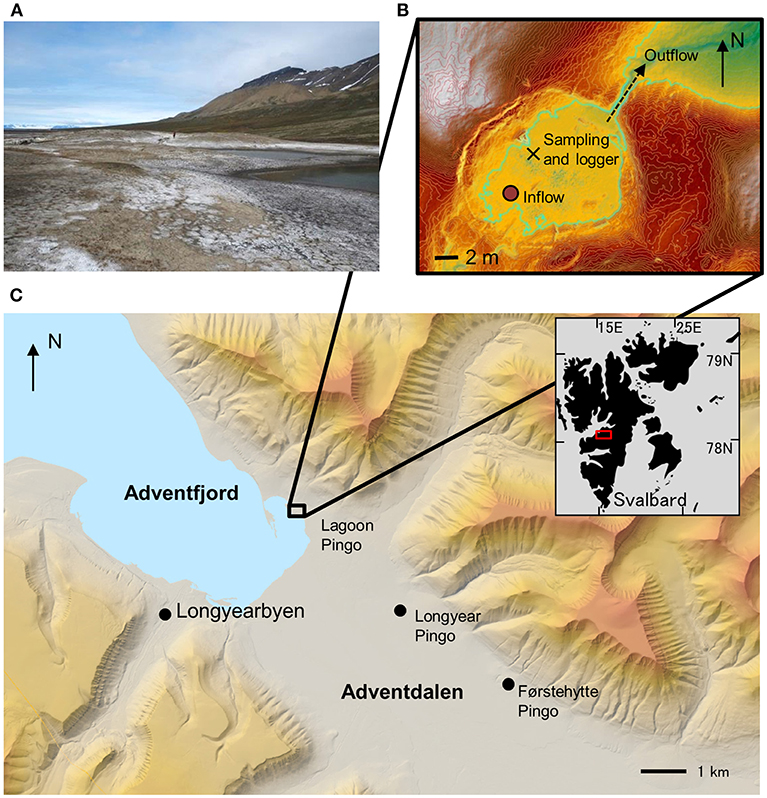
Figure 1. Field Site description. (A) Photograph looking west showing efflorescent salts on surface of uplifted pingo. Note person for scale. (B) Aerial view of pingo pond monitoring site showing principal outflow to northeast, the upwelling inflow, the sampling and instrumentation sites and (green line) the pond level in October. Contours are at 10 cm intervals. (C) Local setting of the pingo in Adventdalen, showing two more open system pingos in the valley floor.

FIGURE 2

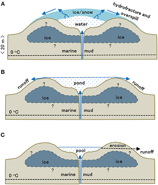
Figure 2. Seasonal development of the Lagoon Pingo system, showing the winter (A), early (B), and late summer (C) configurations. Question marks indicate uncertainty in the sub-surface ground ice distribution.

Field Methods

A Druck pressure transducer was installed in the pond during the 2017 summer to record water level continuously. This was then used in conjunction with a digital elevation model produced at seasonal minimum water level to estimate continuous pond surface area. Other hydrometeorological parameters were available from the nearby Adventdalen Automatic Weather Station maintained by The University Center in Svalbard (see https://www.unis.no/resources/weather-stations/). These data include hourly air pressure, wind speed and air temperature at 10 m elevation for a site 4.5 km away from the pingo in a SSE direction. Liquid precipitation (summer only) was determined at Svalbard Airport, ca. 4 km west.

Electrical conductivity and pond surface temperature were also measured continuously at the same site as the pressure transducer using a Campbell CS547A sensor. Continuous records of water level, surface temperature and electrical conductivity were derived from July 13th until 21st October, 2017 (day of year or “DOY” 164–294). In addition, water samples were collected at the site in April 2016 and March, April, July, August, September and October, 2017. These were used to estimate the dissolved CH₄ and CO₂ concentrations, the major ion chemistry, the concentration of Fe and Mn and the δ¹³C isotopic composition of dissolved methane. Figure 1 shows that sampling was conducted at a single site under the assumption that the pond was well-mixed on account of its small area and exposure to winds. Furthermore, the fluidised, soft muddy bottom of the pond made access to other parts of the pond for sampling rather treacherous. For CH₄ concentration and stable isotope composition, unfiltered samples were collected in pre-cleaned 20 mL crimp-top bottles and stored inverted in the dark at 4°C prior to analysis in the UK up to 2 months later. The same procedure was used for the determination of dissolved inorganic carbon. In-situ dissolved CH₄ measurements were also determined twice (late summer and spring) using a MiniCH₄ detector (Pro-Oceanus, Canada) immediately after factory calibration. The MiniCH₄ results suggested minimal CH₄ change during storage because its results were within 10% of those from the laboratory, and neither technique produced consistently higher values.

For all parameters other than CH₄ and CO₂, samples were filtered using pre-rinsed 0.45 μm Whatman Puradisc Aqua 30 syringe filters. Samples for Fe and Mn analysis were stored in 15 mL Eppendorf Tubes after immediate acidification to pH ~1.7 using reagent grade HNO${}_3^{-}$ (AnalaR 65% Normapur, VWR, IL, USA). Samples for major ions were stored in sterile 15 mL Eppendorf Tubes after filtration and rinsing. The following parameters were collected on-site using Hach HQ40D meters: pH by gel electrode, O₂ by luminescence (detection limit 0.1 mg L⁻¹), Oxidation-Reduction Potential (ORP) by gel electrode. Factory calibrations were used for all but the pH sensor, which was calibrated with the manufacturer's pre-made solutions of pH 4, 7 and 10. ORP data are not presented here as they were only used to prevent collection of oxygenated waters (i.e., waters with positive ORP values) in samples collected from beneath the winter ice lids. Strongly reducing conditions were encountered during the sampling conducted in March and April (ORP down to −300 mV).

Prior to the summer, sampling required drilling through up to 2 m of ice in order to gain access to the underlying water (rather than any partially degassed water discharging from the cracks). Drilling was conducted immediately above the inflow (Figure 1B). Each time this was conducted, pressurized water was encountered, which facilitated sampling through the 7 cm diameter drill hole. To prevent the electrodes from freezing, this water was also pumped through a bespoke flow cell with an internal heating unit. This usually maintained the water at about 7°C, and the inflow temperature was nearly always ca. −0.1°C. Handling these samples in air temperatures down to −30°C was therefore very difficult due to rapid freezing. Syringe filtration was therefore achieved by using hand-warmth to prevent the filter from freezing.

When sampling and monitoring ceased on October 21st a complete aerial survey was undertaken using a DJI Phantom 4 drone, capturing 410 images of 12 Mpx each, yielding a ground resolution of 2.1 cm. The images were processed using Agisoft Photoscan version 1.3.5, employing Structure-from-Motion (SfM) photogrammetry in order to construct a digital elevation model (DEM) (e.g., Mancini et al., 2013; James et al., 2017; Forsmoo et al., 2018). Ground Control Points (GCPs) were derived from the Norwegian Polar Institute's (NPI) aerial photogrammetric survey in 2009 (http://geodata.npolar.no/), resulting in a mean horizontal RMSE of 0.304 m, and a vertical RMSE of 0.176 m. Next, a dense point cloud reconstruction was performed and optimized in PhotoScan, to produce 100,331,290 points representing the surface and then a final 25 × 25 cm DEM (Figure 1B). The DEM was then used to construct an inundation area vs. water level curve after tracing the contours of the terrain surrounding the pond, using ESRI's ArcMap 10.5, and then measuring their planimetric areas. In so doing, the southern and northern outlets of the pond needed to be artificially dammed in order simulate the area of the pond observed in early summer. This testified to the erosion of the soft mud and ice at the two outlets from the pond by early summer runoff.

Laboratory Methods

Analysis of Cl⁻, NO${}_3^{-}$, PO${}_4^{3-}$ and SO${}_4^{2-}$ employed a Dionex ICS90 ion chromatography module calibrated in the range 0–2 mg L⁻¹ for NO${}_3^{-}$ and PO${}_4^{3-}$ and in the range 0–50 mg L⁻¹ for Cl⁻ and SO${}_4^{2-}$ (necessitating dilution). Precision errors for these ions ranged from 0.9% (SO${}_4^{2-}$) to 1.6% (PO${}_4^{3-}$) and the limit of detection (three times the standard deviation of ten blanks) was ≤ 0.05 mg L⁻¹. A Skalar Autoanalyser, was employed for quantification of NH${}_4^{+}$ and then dissolved Si (detection limits 0.1 mg L⁻¹) on a separate, previously unopened 15 mL vial that had been purposely filled to exclude any headspace. Both assays used standard colorimetric methods. Concentrations of cations Ca²⁺, Mg²⁺, Na⁺ and K⁺ were determined by ICP-OES using a Thermo Fisher iCAP 7400 Radial ICP-OES with an internal standard of 1 ppm Y, a limit of detection of 0.07 mg L⁻¹ or better and precision errors ≤ 3.65%. For Sr, Fe and Mn, we employed a Thermo Fisher iCAPQc ICP-MS, with internal standard of 1 ppb Rh, a limit of detection ≤ 0.7 ppb and precision 3.2% or better. Accuracy of each method was assessed by analyzing freshwater certified reference standards throughout the analyses.

Alkalinity was deduced by charge balance calculations involving all of the ions described above. Methane and CO₂ concentrations were determined using a GC-2014 Shimadzu Gas Chromatograph with a methaniser and flame ionization detector, employing a 30 m GS-Q, 0.53 mm internal diameter column with N₂ as a carrier gas at a flow rate of 8 ml/min. The analysis used 100 μL of gas after creating a 5 mL headspace in the sample vial with N₂, and the sample run time was 3 min at 40°C. The limit of CH₄ detection was 10 ppm v as gas, corresponding to an aqueous concentration of ca. 0.3 ppb. The corresponding values for CO₂ were 75 ppm v and 0.2 mg L⁻¹. The precision errors according to certified gas standards (BOC 60% CH₄, 40% CO₂) were always < 1%.

The δ¹³C isotopic composition of dissolved methane also employed a gas headspace equilibration technique after 5 mL sample water was injected into a Viton-stoppered, He-flushed 120 ml glass serum vial. 10 mL of the headspace was then flushed through a 2 mL sample loop, before injection into a 25 m MolSieve column within an Agilent 7890B GC attached to an Isoprime100 Isotope Ratio Mass Spectrometer (IRMS). Analytical precision errors were < 0.3‰ for samples with more than 3 ng C. Due to risk of freezing, samples were crimped immediately and without preservation. Since the delay between sampling during the pre-melt period and analysis was up to 2 months, the δ¹³C of these early samples might be influenced by microbial processes in the sample vial. However, these samples were notable for having almost no turbidity. During summer, great care was taken to avoid suspended sediment being incorporated into the vials. Since this was also challenging, biological effects cannot be discounted for these samples either.

Gas Evasion Modeling

CH₄ and CO₂ evasion fluxes from the pond that formed in the summer period were estimated using the Thin Boundary Layer approach following Wanninkhof (2014). The diffusion-only flux F is given by Equation (1):

$\begin{array}{cc}\begin{array}{r}{F}^{summer}=A\times 0.251\times U_{10}{(Sc/660)}^{-0.5}(C_w-C_a)\end{array}& (1)\end{array}$

Where F^summer (g C h⁻¹) is the outgassing flux when the pond existed during summer, A is the water surface area (m²), established for each water level using the DEM and which decreased from 330 to 180 m². Two empirically-derived constants, 0.251 and 660 enable the gas transfer velocity of a particular gas to be estimated from wind speed. This works best at wind speeds between 3 and 15 ms⁻¹ for reasons discussed by Wanninkhof (2014). U₁₀ is the average wind velocity at 10 m elevation and Sc the unitless, gas-specific and temperature-sensitive Schmidt Number (see Wanninkhof, 2014; Table 1). The difference between the gas concentration in the surface waters of the pond and the atmosphere above it is represented by (C_w – C_a) in g m⁻³. We assumed fixed atmospheric CH₄ and CO₂ partial pressures of 1.935 and 406 ppm v, respectively (www.mosj.no) and then calculated C_a values for each gas using Equation (2):

$\begin{array}{cc}\begin{array}{r}{C}_a=P_{gas}\times \beta \times P_{BARO}\end{array}& (2)\end{array}$

Where β is temperature- and salinity-dependent Bunsen Solubility coefficient calculated using following Yamamoto et al. (1976) and Weiss (1974) for CH₄ and CO₂, respectively and P_BARO is ambient atmosphere barometric pressure. Linear interpolation was used to fill the gaps in C_w for both gases between sampling intervals.

TABLE 1

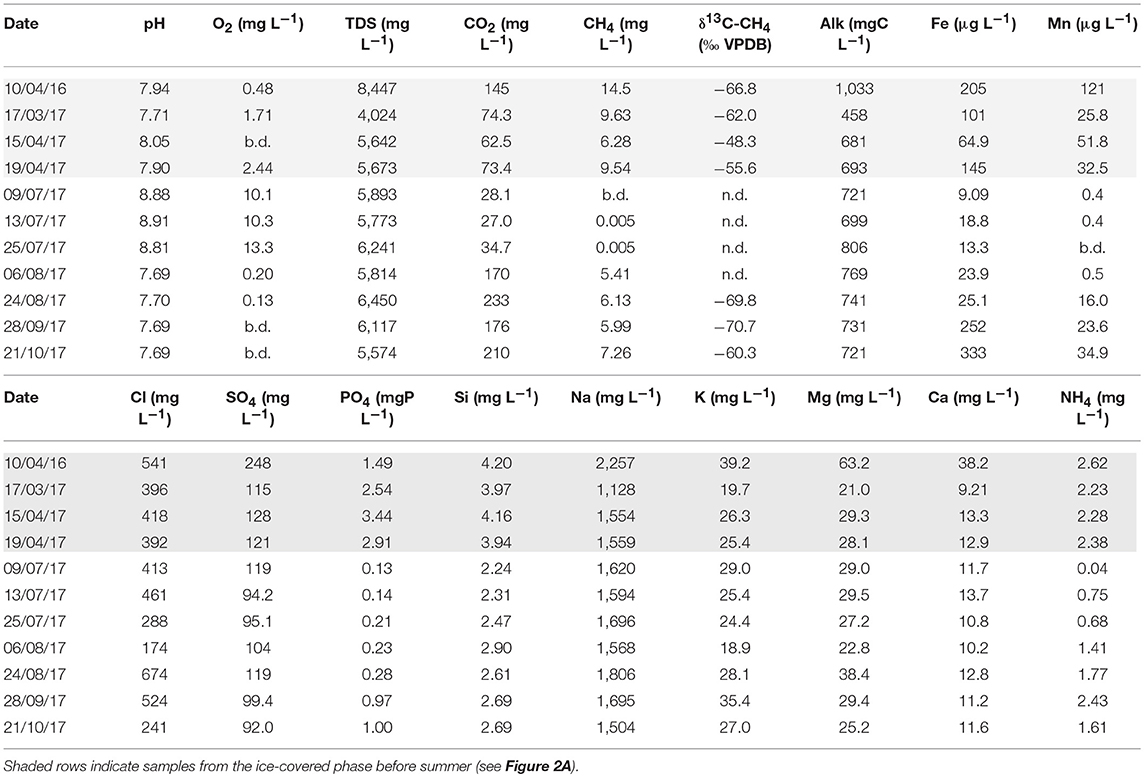
Table 1. Geochemical characteristics of Lagoon Pingo surface waters (“b.d.” means below detection, “n.d.” means not determined).

Non-diffusive evasion, such as ebullition, or bubble transfer to the surface, are not considered by this approach, suggesting that our estimates will be conservative if this process is effective. Ebullition has been observed at the site, but not quantified.

Winter Emission Estimation

The potential contribution of winter methane evasion F^winter was estimated using Equation (3).

$\begin{array}{cc}\begin{array}{r}{F}^{winter}=\overline{Q}\times (C_w-C_a)\end{array}& (3)\end{array}$

Where F^winter units are g C day⁻¹, $\overline{Q}$ is the mean daily water discharge volume and (C_w – C_a) is the difference between the gas concentration of the spring and atmospheric equilibrium. This simple procedure ignores the gas content of the ice lid, which we feel is reasonable given that the ice thickness seemed to remain constant throughout the winter and much of its gas content would have been retained by the residual water during freezing. Values of C_w were 142.8 ± 27.0 (standard error, n = 7) mg CO₂ L⁻¹ and 7.17 ± 0.66 (standard error, n = 7) mg CH₄ L⁻¹), representing the average of all 2017 samples except those collected during July (i.e., when values in the pond were not representative of the inflowing spring due to the high water level). Values for C_a (1.05 mg CO₂ L⁻¹ and 7.85 × 10⁻⁵ mg CH₄ L⁻¹) were calculated in the same manner as in section Gas Evasion Modelling using a fixed salinity and temperature of 5 p.s.u and 0°C, respectively. The mean spring discharge was assumed to be 0.36 L s⁻¹ (31 m³ day⁻¹) for reasons that are discussed in section Methane Sources and Fluxes to the Atmosphere.

Results

In winter, an ice blister with a convex upwards surface ca. 1 m thick formed over the pingo outflow (Figure 2A). When punctured during the sampling in March and April, the blister would discharge water for several hours at an initial flow rate of ca. 1 L s⁻¹ before refreezing of the ice caused closure. The volume of water stored beneath the blister at the time could not be discerned, but is likely to have been broadly equivalent to the pond that formed at the start of the summer once the ice blister had ablated. Later, presumably in early June (when the site was inaccessible), the ice blister collapsed and ablated completely to reveal the pond. This pond persisted until late October, when freezing commenced again. Local variations in air temperature (not shown) involved a clear switch to sustained, positive air temperatures on ca. 7th June 2017 (DOY 158), when the ice lid likely ablated. As a consequence, an influx of local snowmelt and ice melt from the overlying blister occurred at this time, resulting in seasonal maximum water storage in the pond between mid-June and the 9th July (DOY 190) sampling visit. Thereafter, Figure 3A shows that sustained, positive air temperatures generally persisted until early October (DOY 279), during which a slow drainage of the pond took place, with the exception of a slight increase in water level commencing during late August (DOY 234). Throughout the observation period, the outflow rate and thus the pond level were influenced by the erosion of the soft mud banks, lowering the base level of the outflow points by ca. 20 cm and causing the pond to reach seasonal minimum levels at the very end of the observation period. No major changes in the inflow rate were discernible. However, the small increase in water level in late August was most-likely linked to increased inflow, because although it was preceded by appreciable rainfall (ca. 19 mm) in the interval July 13th−20th (DOY 194–201), other rainfall events of equivalent magnitude in late August and late September were not associated with any subsequent changes in water level.

FIGURE 3

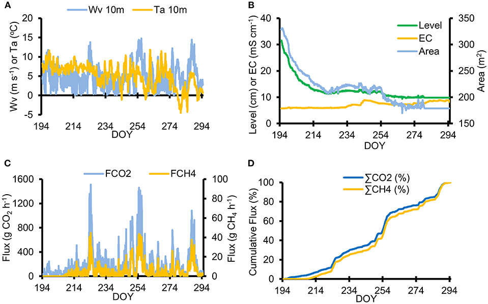
Figure 3. Hourly meteorological conditions and modeled CH₄ and CO₂ evasion fluxes from 13th July (DOY 194) until 21st October (DOY 294) 2017. (A) Wind velocity and air temperature at 10 m elevation (“WV” and “Ta,” respectively); (B) pond level (“Level”), area (“Area”) and electrical conductivity (“EC”); (C) Evasion flux of CO₂ and CH₄ (FCO₂ and FCH₄, respectively), and (D) Percentage distribution of the cumulative evasion flux of both gases [“∑CO₂ (%)” and “∑CO₂ (%)”].

Figure 3B shows that the electrical conductivity (EC) of the pond (5–8 mS cm⁻¹) was far in excess of values reported in natural surface waters of the region (i.e., up to 0.4 mS cm⁻¹: see Hodson et al., 2016 and Rutter et al., 2011), and therefore indicative of highly concentrated water flowing into the pond. Since only minor changes in EC were recorded (relative to the significant variations in pond water level) there seems to have been little mixing between the groundwater spring flowing into the base of the pond and either local surface runoff (EC = < 0.4 mS cm⁻¹), or the sea (sea water EC at 0°C = ~30 mS cm⁻¹), which approaches the base of the pingo when spring tides are pushed ashore by winds from the south. The small increase in pond level during August described above was coincident with a gradual increase in the EC (Figure 3B), which therefore suggests the increased inflow of concentrated groundwaters occurred.

Table 1 shows that the dissolved O₂ levels in the pingo pond increased to values typical of well-aerated surface waters (i.e., >10 mg L⁻¹) or even super-saturated (13 mg L⁻¹) in the case of the 25th July sample. These values were far in excess of those recorded either prior to the summer, or from August onwards. Trace quantities of O₂ were reported on occasion at these times, although in March and April, this probably reflected the introduction of O₂ whilst transferring sample to the flow cell during difficult (freezing) sampling conditions. Methane concentrations were greatest (14.5 mg L⁻¹ in April 2016 and up to 9.63 mg L⁻¹ in 2017) when the system was entombed beneath the ice lid (Figure 4A). Concentrations then dropped to below the limit of detection during July, before recovering slightly thereafter to between 5 and 7 mg L⁻¹. Figure 4A also shows that dissolved CO₂ concentrations demonstrated similar variability to CH₄, because minimum values occurred during July, but unlike CH₄, concentrations in late summer exceeded those in March or April. Therefore, the ratio of CH₄ to CO₂ was greatest prior to the onset of melt, indicating important differences in the dynamics of CH₄ and CO₂ over the entire year. However, these differences were not captured in during the shorter period of monitoring and evasion modeling that commenced in July.

FIGURE 4

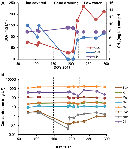
Figure 4. Time series observations of the principal water quality results given in Table 1. (A) pH and the dissolved gases, (B) major ions.

Table 1 and Figure 4 show the aqueous water quality parameters collected at the site. The pH values were in the 7.7–8.9 range, with the highest pH values being observed when the water was most oxygenated (in mid-July). Marine salts were an important source of ions, because Cl⁻ concentrations were 400 mg L⁻¹ or more. However, the period of high pond water levels clearly shows Cl⁻ dilution occurred in early summer (DOY 194–218), suggesting an influx of snowmelt or other meteoric water from the vicinity of the pond. The cation results show that Na⁺ concentrations were far in excess of Cl⁻ and all the other cations, because they were generally >1,100 mg L⁻¹. Other notable features of the water quality parameters included the absence of detectable NO${}_3^{-}$, yet the occurrence of SO${}_4^{2-}$ concentrations clearly in excess of that which would be expected from a marine source (according to the Cl⁻ concentrations in the pond and a typical sea water SO${}_4^{2-}$/Cl⁻ ratio of 0.14). Dissolved Fe and Mn concentrations were both at the sub-ppm level, whilst Si was up to 4 mg L⁻¹ before summer and 2–3 mg L⁻¹ thereafter (see Table 1).

Although NO${}_3^{-}$ was consistently below detection limits, NH${}_4^{+}$ and PO${}_4^{3-}$ were observed at mg L⁻¹ levels far in excess of surface waters, whose nutrients are typically at the μg L⁻¹ level and dominated by NO${}_3^{-}$ (e.g., Rutter et al., 2011). However, Figure 4B shows that strong depletion in both NH${}_4^{+}$ and PO${}_4^{3-}$ occurred during July, before recovering gradually in August and September. Whilst concentrations of NH${}_4^{+}$ recovered to pre-summer levels toward the end of the sampling period, PO${}_4^{3-}$ concentrations remained below 1 mg L⁻¹.

Flux estimates from the thin boundary layer calculations using an hourly time step are shown in Figures 3C,D. Error analysis suggested that the uncertainty (not shown) was ca. 28% for CO₂ and 22% for CH₄. A strong correlation existed between the CO₂ and CH₄ fluxes (Pearson's Correlation Coefficient of 0.99, p < 0.01) according to the instantaneous flux estimates from sampling days after the loss of the ice cover (n = 6). However, this correlation is limited to the period when both gas concentrations demonstrated similar temporal variations once detectable CH₄ levels returned to the pond (especially after 9th August or DOY 218). According to the hourly evasion flux estimates, four periods of high winds are discernible in Figure 3C (DOYs 223–228; 249–251; 254–259 and 285–291), each adding significant increments to the cumulative seasonal fluxes shown in Figure 3D. These 22 days contributed more than 50% of the total 100 days flux of both gases.

Discussion

Geochemical Characteristics of the Spring

The water quality data presented in Table 1 indicates that the spring discharging from Lagoon Pingo is clearly influenced by the underlying marine sediments, although only modest concentrations of Cl⁻ result in the pond. Therefore, the majority of the groundwater entering its bed via the spring is more likely of meteoric origin. This means the simple expulsion of marine sediment pore waters undergoing freezing during uplift of the lagoon seems unlikely to be solely responsible for the spring. A ground water flowpath through fractured sandstone bedrock beneath the permafrost has been reported in Adventdalen (Braathen et al., 2012; Huq et al., 2017) and is thought to be connected to pockmarks on the fjord floor (Roy et al., 2014). We therefore argue that the pingo spring is connected to this aquifer, albeit resulting in a very minor discharge, and that it may exploit a flowpath first established during the formation of the pockmark swarms further out in the fjord, which are thought to pre-date isostatic uplift and permafrost aggradation (Portnov et al., 2016). Other geochemical characteristics of the spring indicate frequent over-saturation with respect to several carbonate mineral phases (calcite, dolomite and siderite: data not shown) according to geochemical speciation modeling with Phreeqc Software (Parkhurst, 1980). Mineral precipitation reactions, as well as potential ion exchange processes, therefore greatly influence the cation composition of the spring water. This, coupled with significant rates of alkali feldspar (e.g., Albite) weathering (Yde et al., 2008), lead to a clear dominance of Na⁺ at concentrations in excess of those that would be expected from marine pore waters (given their modest contribution to Cl⁻). With respect to the anion composition, NO${}_3^{-}$ is almost certain to have been removed by denitrification, but it is unclear whether the modest SO${}_4^{2-}$ concentrations have been influenced by SO₄ reduction, although black sulfide precipitates circulating in the pond bed clearly indicated that some SO₄ reduction was likely taking place, as did the occasional odor of H₂S. Since the ratios of SO${}_4^{2-}$ to Cl⁻ (average 0.32 ± 0.12 using Table 1 data) are in excess of those that may be expected from the standard marine water (ie ca. 0.14), SO${}_4^{2-}$ acquisition from sulfide oxidation and/or gypsum dissolution appears likely to have occurred prior to the onset of any sulfate reduction. Further studies will therefore need to examine the sulfur cycle in greater detail. However, the development of high SO${}_4^{2-}$ and Na⁺ concentrations following rock weathering are well-known from studies of surface waters in the area (Yde et al., 2008; e.g., Rutter et al., 2011) and do not allow us to reject the hypothesis that Lagoon Pingo spring waters are the result of high rock-water contact in a bedrock aquifer within sandstones and shales.

Seasonal Hydrological and Biogeochemical Changes in the Pingo Pond

Our study reveals how the simple seasonal progression of hydrological and biogeochemical conditions at the site are controlled largely by the interplay between an anoxic, methane-rich inflow to the bed of the pond, diluted by meltwater from a salty ice lid and local snowmelt during early summer (Figure 4B), and the outflow. Since very little rainfall occurred at this site, the seasonal changes in Figures 3B, 4A show that the groundwater inflow gradually allowed gas-rich water to dominate the pond, once the meltwaters had drained from it in early summer. Erosion of the pond outlet reduced the volume of the pond as well, which hastened the runoff of the aerated melt water and made it easier for recent groundwater inflow to dominate. Turbulent mixing will also have been facilitated by the shallower depths. As a consequence, the flux of greenhouse gases to the atmosphere increased in spite of the pond surface area decreasing. Simple hydrological changes therefore played a cardinal role in the methane and carbon dioxide outgassing rate of the system at shorter time scales. Figures 3B,D show that CH₄ evasion was negligible until the pond level had dropped by 15 cm. After this, gas concentrations increased and strong, shorter-term (hourly to daily) variations in methane and carbon dioxide outgassing occurred in response to meteorological forcing (Figures 3C, 4A).

Prior to summer, the ventilation of the anoxic water was far from continuous, because it required fracture of the ice lid. This event has been witnessed at a total of four pingos in the local Adventdalen area, and is evidenced by the formation of large icings downstream from the fracture point. It is also observable at open system pingos in two other major valleys in the region (Grøndalen and Reindalen). The escape of methane to the atmosphere therefore occurs during winter as well as summer, but the winter freezing results in an overlying ice blister that dilutes these systems in early summer (especially if a pond is present) because solute rejection and rapid evasion minimize the CH₄ and CO₂ content of the ice as it forms the lid.

Differences between the ratio of CH₄ and CO₂, as well as non-conservative nutrient dynamics suggest that the biogeochemical conditions within the pingo pond were also influenced by biological activity. For example, the assimilation of NH${}_4^{+}$ and PO${}_4^{3-}$, both present at far greater concentrations than natural surface waters in Svalbard (e.g., Hodson et al., 2005), almost certainly occurred, because biofouling of the hydrological sensors necessitated their cleaning and there was a visible algal biomass in the center of the pond by the end of the summer. Autotrophic production (photosynthesis) therefore most likely reduced the CO₂, PO${}_4^{3-}$, and NH${}_4^{+}$ content of the pond to seasonal minimum values, as is discernible in Figure 4B. Since CH₄ was undetectable for a while (9th July, 2017), it is also possible that methanotrophy was being influential at this time.

Methane Sources and Fluxes to the Atmosphere

Although local production of methane in the bottom sediments of the pond was feasible, methanogenesis is known to occur in the sediments and bedrock just beneath the permafrost in Adventdalen (Huq et al., 2017). Table 1 also shows that biogenic methane dominates the pond in late summer, on account of the low δ¹³C-CH₄ values that approach −71 ‰ VPDB (Schoell, 1980). These values are therefore consistent with the supply of biogenic methane from a sub-permafrost groundwater flowing into the bottom of the pond. Furthermore, these values cannot be attributed to the thermogenic methane that is known to be diffusing upwards from depths in excess of 400 m in the region, and which have an end-member composition of ca. −45 ‰ VPDB (Huq et al., 2017). However, Table 1 shows that the δ¹³C-CH₄ values during the period of ice cover were markedly higher (less negative) than those from late summer, indicating that a greater proportion of thermogenic methane was possible. However, oxidation and/or methanotrophy could also have been influential beneath the ice lid during winter. Post-sampling oxidation of the methane might also have contributed to this difference, although this seems unlikely because these samples contained no visible turbidity and there was no evidence for significant CH₄ concentration change during storage. Establishing how much oxidation occurs beneath the ice cover during winter is difficult, however. For example, the occasional detection of O₂ during March and April might indicate partial oxidation, but this could instead have been an artifact of the electrode measurements at this time of year (which required pumping water to a heated flow cell. Measurements in summer simply required immersion of the electrodes into the water). Furthermore, the possibility that more biogenic methane is present during summer seems plausible and has been deduced from the δ¹³C-CH₄ of summer outflows from an Icelandic glacier (Burns, 2016). However, this alternative explanation is difficult to invoke at Lagoon Pingo, because the concentrations of CH₄ were lower during summer than during the pre-melt period. Therefore, it seems most plausible to conclude that isotopic fractionation affects the δ¹³C-CH₄ values when large volumes of the gas were stored beneath the ice lid at their seasonal maximum concentration. This means that while the importance of biogenic methane is clear at Lagoon Pingo, the importance of thermogenic methane cannot be established from our data.

Estimates of the total pond evasion fluxes of CH₄ and CO₂ from the pingo system are shown in Table 2, based initially upon the 100 days of summer monitoring and evasion modeling. For methane, the modeled flux is 13 kg ± 2.9 CH₄ (i.e., 0.13 ± 0.03 kg CH₄ day⁻¹). This could have been sustained by the complete evasion of methane from a constant inflow of just 0.21 L s⁻¹ carrying a CH₄ concentration of 7.18 mg L⁻¹, the average concentration of all samples thought to be most representative of the inflowing spring (i.e., the average of all samples other than those from July). For CO₂, the flow required to maintain the modeled evasion flux of 440 ± 121 kg CO₂ is greater (0.36 L s⁻¹) when the same samples are used to calculate the average inflow concentration (142.8 mg L⁻¹). Variations in the relative concentrations of the two gases through time might contribute to these different estimates of spring inflow into the bottom of the pond. However, CH₄ is likely to be most sensitive to removal processes in the pond, because its concentrations are furthest from equilibrium with respect to the atmosphere. Therefore, we assumed that the higher value of 0.36 L s⁻¹ was most representative of the actual inflow into the pond.

TABLE 2

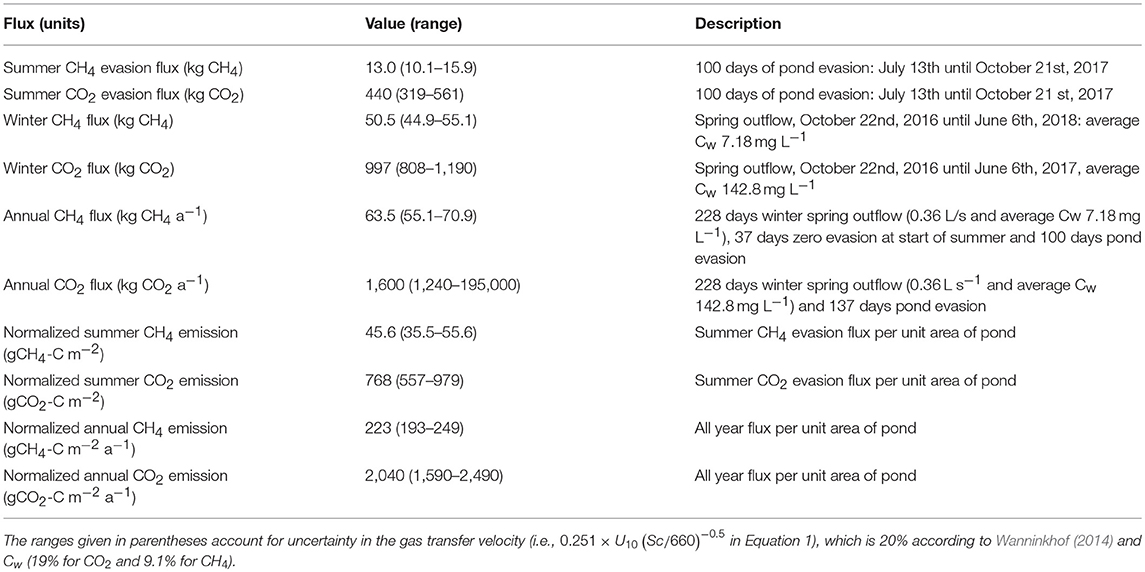
Table 2. Fluxes of CH₄ and CO₂ estimated by the study and including the summer emissions from the pond and the winter emissions from the spring.

An estimate of methane emission for the entire year was derived by adding the winter emission rate to the summer evasion rate from the pond. In so doing, we assumed from meteorological records that the pond formed on June 7th, and that zero CH₄ evasion occurred from this date until July 13th, when dissolved CH₄ was detectable in pond surface waters once more. For the preceding winter period (defined as October 22nd, 2016 until June 7th, 2017) we followed the calculations outlined in section Winter Emission Estimation, using the estimate of average spring discharge (0.36 L s⁻¹) described above and the difference between average gas concentrations and atmospheric equilibrium concentration values (see section Winter Emission Estimation). However, unlike CH₄, the CO₂ evasion between June 7th and July 13th could not be assumed negligible because concentrations in the pond were in excess of the equilibrium concentrations (i.e., C_a in Equation 1). Therefore, we used a scaling factor of 1.37 to account for the extra 37 days not accounted for prior to our 100 days of CO₂ evasion modeling. Table 2 shows that the contribution to total annual emission during the winter can be potentially very significant, representing 80 and 62% of the total annual flux estimates for CH₄ and CO₂, respectively. More insights into the frequency of cracking and outflow through the ice lid should be sought in order to better understand this period of emission. Also, more effort is required to estimate the variability of groundwater discharge at this site and others like it. The frequent, sulfurous odor at Lagoon Pingo and two other open system pingos in the valley when no outflows are discernible, suggests that gas emissions through the cracks in the ice lid should also be considered.

When normalized for surface area, the pingo pond emissions during the summer can be compared to chamber measurements that are used to describe active layer emissions. Data in Table 2 show that the pingo pond methane evasion flux in summer of 46 gCH₄-C m⁻² exceeds values for local wetlands in Adventdalen, whose (median) rates are in the range 1–2 gCH₄-C m⁻² (Pirk et al., 2017). The differences are clearly increased when the winter emissions from the pingo are included, resulting in an annual methane emission of ca. 223 gCH₄-C m⁻². CO₂ emissions (768 gCO₂-C m⁻² from the pingo pond in summer) are difficult to compare to regional wetlands, owing to strong variations in primary production and respiration, and also differences between wetlands and other types of soil. However, in a study conducted in meadow and heathlands of Adventdalen, Björkman et al. (2010) estimated annual emission rates of up to 600 gCO₂-C m⁻², dominated by summer. Therefore, during summer, Lagoon Pingo constitutes an important local hotspot for the emission of CH₄ but less so for CO₂. By late winter, it probably represents the only significant emission source in the immediate vicinity. Gas emissions by groundwater seepages associated with both pingos and springs in coastal Arctic lowlands undergoing isostatic uplift are therefore worthy of inclusion in their greenhouse gas budgets. Their further study will also provide a means for improving our understanding of the biogeochemical processes occurring beneath permafrost.

Conclusions

This study demonstrates how significant contributions to landscape methane evasion can be made by sub-permafrost ground water that is able to discharge at the land surface following minimal interaction with water and soil ecosystems along the way. In West Spitsbergen, open system pingos are important conduits for these fluids, and their genesis is linked to isostatic uplift and permafrost aggradation in response to ice sheet retreat (in this case the Barents Ice Sheet) over the last 10 000 years. Other features that enable the rapid escape of methane from the sea floor, namely pockmarks, have also been associated with ice sheet retreat in this region (e.g., Portnov et al., 2016). Our study suggests that the uplift of pockmarks from shallow glacio-marine environments can be responsible for open system pingo formation during subsequent permafrost aggradation, because the ground water migration route already exists. In our case study of one such pingo (Lagoon Pingo, Adventdalen), we have demonstrated the occurrence of high methane concentrations (up to 14.4 mg L⁻¹) and revealed a strong seasonality in emission rates. This seasonality is due to early summer melt water ingress into the pond that forms at the center of the pingo, causing negligible emissions until the summer melt layer is replaced by new groundwater inflow. This water exchange process is accelerated by erosion of the small channels that drain the pond, resulting in appreciable rates of gas evasion from early August until the start of winter refreezing (46 gCH₄-C m⁻² a⁻¹ and 768 gCO₂-C m⁻² a⁻¹). During winter, evasion is associated with sporadic outflows and thermal or hydrostatic cracking of the ice lid. Further studies of the winter emission rates are necessary because they can constitute the majority of the annual CH₄ and CO₂ emissions according to our measurements. However, comparison of the emission rates of both gases to local wetlands and soils suggests that only the CH₄ emissions are important contributors to landscape greenhouse gas emissions.

Data Availability

The raw data supporting the conclusions of this manuscript but not presented above will be made available by the authors to any qualified researcher. These data include the meteorological and hydrological time series used in the pond evasion modeling and the digital elevation model. All other data can be found in this manuscript.

Author Contributions

AH and AN collected the samples and the on-site geochemical data. EH conducted the UAV survey and processed the data. The laboratory analysis was undertaken by KR and AT. AH conducted the evasion modeling and wrote the manuscript, with equal editorial input from AN, HC, KR, EH, and AT after the first draft.

Conflict of Interest Statement

The authors declare that the research was conducted in the absence of any commercial or financial relationships that could be construed as a potential conflict of interest.

Acknowledgments

The authors acknowledge the Joint Programming Initiative (JPI-Climate Topic 2: Russian Arctic and Boreal Systems) Award No. 71126, UK Natural Environment Research Council grant NE/M019829/1, Research Council of Norway grant No. 244906 and a Royal Geographical Society (with IBG) Ralph Brown Memorial Award (2017). Sarah Sapper, Molly Peek, and Peter Betlem are thanked for their field assistance during the summer.

References

Anthony, K. M. W., Anthony, P., Grosse, G., and Chanton, J. (2012). Geologic methane seeps along boundaries of Arctic permafrost thaw and melting glaciers. Nat. Geosci. 5, 419–426. doi: 10.1038/ngeo1480

CrossRef Full Text | Google Scholar

Björklund, A. (1990). Methane venting as a possible mechanism for glacial plucking and fragmentation of Precambrian crystalline bedrock. Geologiska Föreningen i Stockholm Förhandlingar 112, 329–331. doi: 10.1080/11035899009452731

CrossRef Full Text | Google Scholar

Björkman, M. P., Morgner, E., Björk, R. G., Cooper, E. J., Elberling, B., and Klemedtsson, L. (2010). A comparison of annual and seasonal carbon dioxide effluxes between sub-Arctic Sweden and High-Arctic Svalbard. Polar Res. 29, 75–84. doi: 10.1111/j.1751-8369.2010.00150.x

CrossRef Full Text | Google Scholar

Braathen, A., Bælum, K., Christiansen, H. H., Dahl, T., Eiken, O., Elvebakk, H., et al. (2012). The Longyearbyen CO₂ Lab of Svalbard, Norway—initial assessment of the geological conditions for CO₂ sequestration. Nor. J. Geol. 92, 353–376.

Google Scholar

Burns, R. K. (2016). Cryogenic Carbon Cycling at an Icelandic Glacier. PhD thesis, Lancaster University. 275.

Forsmoo, J., Anderson, K., Macleod, C. J. A., Wilkinson, M. E., and Brazier, R. (2018). Drone-based structure-from-motion photogrammetry captures grassland sward height variability. J. Appl. Ecol. 55, 2587–2599. doi: 10.1111/1365-2664.13148

CrossRef Full Text | Google Scholar

Forwick, M., Baeten, N. J., and Vorren, T. O. (2009). Pockmarks in Spitsbergen fjords. Nor. J. Geol. 89, 65–77.

Google Scholar

Gentz, T., Damm, E., von Deimling, J. S., Mau, S., McGinnis, D. F., and Schlüter, M. (2014). A water column study of methane around gas flares located at the West Spitsbergen continental margin. Cont. Shelf Res. 72, 107–118. doi: 10.1016/j.csr.2013.07.013

CrossRef Full Text | Google Scholar

Gilbert, G. L., Cable, S., Thiel, C., Christiansen, H. H., and Elberling, B. (2017). Cryostratigraphy, sedimentology, and the late Quaternary evolution of the Zackenberg River delta, northeast Greenland. Cryosphere 11, 1265–1282. doi: 10.5194/tc-2016-299

CrossRef Full Text | Google Scholar

Gilbert, G. L., O'Neill, H. B., Nemec, W., Thiel, C., Christiansen, H. H., and Buylaert, J. P. (2018). Late Quaternary sedimentation and permafrost development in a Svalbard fjord-valley, Norwegian high Arctic. Sedimentology 65, 2531–2558. doi: 10.1111/sed.12476

CrossRef Full Text | Google Scholar

Hodson, A., Nowak, A., and Christiansen, H. H. (2016). Glacial and periglacial floodplain sediments regulate hydrologic transfer of reactive iron to a high arctic fjord. Hydrol. Proc. 30, 1219–1229. doi: 10.1002/hyp.10701

CrossRef Full Text | Google Scholar

Hodson, A. J., Mumford, P. N., Kohler, J., and Wynn, P. M. (2005). The High Arctic glacial ecosystem: new insights from nutrient budgets. Biogeochemistry 72, 233–256. doi: 10.1007/s10533-004-0362-0

CrossRef Full Text | Google Scholar

Hong, W. L., Sauer, S., Panieri, G., Ambrose, W. G., James, R. H., Plaza-Faverola, A., et al. (2016). Removal of methane through hydrological, microbial, and geochemical processes in the shallow sediments of pockmarks along eastern Vestnesa Ridge (Svalbard). Limnol. Oceanogr. 61, S324–S343. doi: 10.1002/lno.10299

CrossRef Full Text | Google Scholar

Humlum, O. (2005). Holocene permafrost aggradation in Svalbard. Geol. Soc. London. Spec. Publications 242, 119–129. doi: 10.1144/GSL.SP.2005.242.01.11

CrossRef Full Text | Google Scholar

Huq, F., Smalley, P. C., Mørkved, P. T., Johansen, I., Yarushina, V., and Johansen, H. (2017). The longyearbyen CO₂ lab: fluid communication in reservoir and caprock. Int. J. Greenhouse Gas Control 63, 59–76. doi: 10.1016/j.ijggc.2017.05.005

CrossRef Full Text | Google Scholar

James, M. R., Robson, S., d'Oleire Oltmanns, S., and Niethammer, U. (2017). Optimising UAV topographic surveys processed with structure-from-motion: ground control quality, quantity and bundle adjustment. Geomorphology 280, 51–66. doi: 10.1016/j.geomorph.2016.11.021

CrossRef Full Text | Google Scholar

Liestøl, O. (1996). Open system pingos in Spitsbergen. Norsk Geogr. Tidsskr. 50, 81–84. doi: 10.1080/00291959608552355

CrossRef Full Text | Google Scholar

Mancini, F., Dubbini, M., Gattelli, M., Stecchi, F., Fabbri, S., and Gabbianelli, G. (2013). Using unmanned aerial vehicles (UAV) for high-resolution reconstruction of topography: the structure from motion approach on coastal environments. Remote Sens. 5, 6880–6898. doi: 10.3390/rs5126880

CrossRef Full Text | Google Scholar

Mau, S., Römer, M., Torres, M. E., Bussmann, I., Pape, T., Damm, E., et al. (2017). Widespread methane seepage along the continental margin off Svalbard-from Bjørnøya to Kongsfjorden. Nat. Sci. Rep. 7:42997. doi: 10.1038/srep42997

PubMed Abstract | CrossRef Full Text | Google Scholar

Myhre, C. L., Ferré, B., Platt, S. M., Silyakova, A., Hermansen, O., Allen, G., et al. (2016). Extensive release of methane from Arctic seabed west of Svalbard during summer 2014 does not influence the atmosphere. Geophys. Res. Lett. 43, 4624–4631. doi: 10.1002/2016GL068999

CrossRef Full Text | Google Scholar

Orvin, A. K. (1944). Litt om kilder på Svalbard. Nor. Geogr. Tidsskr. 10, 1–26. doi: 10.1080/00291954408621804

CrossRef Full Text | Google Scholar

Parkhurst, D. L. (1980). PHREEQC; a computer program for geochemical calculations. US Geol. Surv. Wat. Resour. Investig. Rep. 80, 1–195.

Pirk, N., Mastepanov, M., López-Blanco, E., Christensen, L. H., Christiansen, H. H., Hansen, B. U., et al. (2017). Toward a statistical description of methane emissions from arctic wetlands. Ambio 46, 70–80. doi: 10.1007/s13280-016-0893-3

PubMed Abstract | CrossRef Full Text | Google Scholar

Portnov, A., Vadakkepuliyambatta, S., Mienert, J., and Hubbard, A. (2016). Ice-sheet-driven methane storage and release in the Arctic. Nat. Comm. 7:10314, doi: 10.1038/ncomms10314

CrossRef Full Text | Google Scholar

Roy, S., Hovland, M., Noormets, R., and Olaussen, S. (2015). Seepage in Isfjorden and its tributary fjords, West Spitsbergen. Mar. Geol. 363, 146–159. doi: 10.1016/j.margeo.2015.02.003

CrossRef Full Text | Google Scholar

Roy, S., Senger, K., Braathen, A., Noormets, R., Hovland, M., and Olaussen, S. (2014). Fluid migration pathways to seafloor seepage in inner Isfjorden and Adventfjorden, Svalbard. Nor. J. Geol. 94, 99–119.

Google Scholar

Rutter, N., Hodson, A., Irvine-Fynn, T., and Solås, M. K. (2011). Hydrology and hydrochemistry of a deglaciating high-Arctic catchment, Svalbard. J. Hydrol. 410, 39–50. doi: 10.1016/j.jhydrol.2011.09.001

CrossRef Full Text | Google Scholar

Schoell, M. (1980). The hydrogen and carbon isotopic composition of methane from natural gases of various origins. Geochim. Cosmochim. Acta 44, 649–661. doi: 10.1016/0016-7037(80)90155-6

CrossRef Full Text | Google Scholar

Smith, L. M., Sachs, J. P., Jennings, A. E., Anderson, D. M., and DeVernal, A. (2001). Light δ¹³C events during deglaciation of the East Greenland continental shelf attributed to methane release from gas hydrates. Geophys. Res. Lett. 28, 2217–2220. doi: 10.1029/2000GL012627

CrossRef Full Text | Google Scholar

Wallmann, K., Riedel, M., Hong, W. L., Patton, H., Hubbard, A., Pape, T., et al. (2018). Gas hydrate dissociation off Svalbard induced by isostatic rebound rather than global warming. Nat. Comm. 9:83. doi: 10.1038/s41467-017-02550-9

PubMed Abstract | CrossRef Full Text | Google Scholar

Wanninkhof, R. (2014). Relationship between wind speed and gas exchange over the ocean revisited. Limnol. Oceanogr. Methods 12, 351–362. doi: 10.4319/lom.2014.12.351

CrossRef Full Text | Google Scholar

Weiss, R. F. (1974). Carbon dioxide in water and seawater: the solubility of a non-ideal gas. Mar. Chem. 2, 203–215. doi: 10.1016/0304-4203(74)90015-2

CrossRef Full Text | Google Scholar

Weitemeyer, K. A., and Buffett, B. A. (2006). Accumulation and release of methane from clathrates below the Laurentide and Cordilleran ice sheets. Glob. Planet. Change 53, 176–187. doi: 10.1016/j.gloplacha.2006.03.014

CrossRef Full Text | Google Scholar

Yamamoto, S., Alcauskas, J. B., and Crozier, T. E. (1976). Solubility of methane in distilled water and seawater. J. Chem. Eng. Data 21, 78–80. doi: 10.1021/je60068a029

CrossRef Full Text | Google Scholar

Yde, J. C., Riger-Kusk, M., Christiansen, H. H., Knudsen, N. T., and Humlum, O. (2008). Hydrochemical characteristics of bulk meltwater from an entire ablation season, Longyearbreen, Svalbard. J. Glaciol. 54, 259–272. doi: 10.3189/002214308784886234

CrossRef Full Text | Google Scholar

Yoshikawa, K. (1993). Notes on open system pingo ice, Adventdalen, Spitsbergen. Permafrost Periglac. 4, 327–334. doi: 10.1002/ppp.3430040405

CrossRef Full Text | Google Scholar

Yoshikawa, K., and Harada, K. (1995). Observations on nearshore pingo growth, Adventdalen, Spitsbergen. Permafrost Periglac. 6, 361–372. doi: 10.1002/ppp.3430060407

CrossRef Full Text | Google Scholar