A Stratigraphic Approach to Inferring Depositional Ages From Detrital Geochronology Data

1. Introduction

The age of a sedimentary deposit is no older than its youngest constituent. This fact, and the recent proliferation of detrital geochronology data to understand sedimentary provenance, have expanded the use of maximum depositional ages (MDAs) to constrain the ages of sedimentary deposits. With MDAs, researchers seek to limit the age of an otherwise undateable sedimentary deposit (e.g., a sandstone) using the ages of individual mineral grains, most commonly U-Pb ages of zircons determined by Laser Ablation-Inductively Coupled Plasma-Mass Spectrometry (LA-ICP-MS). The challenge to this approach is transforming the many individual dates of a detrital zircon study (tens to hundreds of grains are often dated per sample, see Sharman et al., 2018; Coutts et al., 2019) to a single measure of the maximum age of the deposit. Analytical and geologic uncertainty in dating methods cause variability about the “true” age of crystallization, such that any given measured age may be scattered about the true age of the rock. Repeated processing of samples in mineral separation facilities also introduces the possibility of potential contamination, as a single misplaced grain of sand could skew results. The imperfection of geologic chronometers means that in the case of radiometric dates, parent or daughter isotopes may be lost, resulting in an incorrect or inaccurate calculation of an age. In response to these challenges, a variety of methods have been developed to aggregate a suite of measured ages from a single detrital sample into a single estimate of the maximum age of the deposit (Dickinson and Gehrels, 2009; Coutts et al., 2019).

In addition to being no older than its youngest constituent, the age of a sedimentary deposit is bracketed by the ages of deposits above and below it in a stratigraphic succession. A Geologist would refer to this as the principle of superposition. A Bayesian Statistician would call this valuable prior information. Superposition and Bayesian statistics have long been used to refine inferences about deposit ages that are based on geochronology (Naylor and Smith, 1988; Buck et al., 1992; Christen et al., 1995). The utility of these methods has resulted in the development of a number of computational tools to enable routine Bayesian analysis of suites of (primarily) radiocarbon ages (e.g., Blaauw and Christen, 2005; Haslett and Parnell, 2008; Parnell et al., 2008; Bronk Ramsey, 2009; Blaauw, 2010; Blaauw and Christeny, 2011). Most commonly these tools are employed to make probabilistic assessments of the age of sedimentary intervals between dated horizons that record environmental changes of interest (Parnell et al., 2011). Radiocarbon calibration results in complicated probabilities of age, which is perhaps part of the reason for the popularity of Bayesian methods (Parnell et al., 2011). Inferring depositional ages from detrital geochronology data provides a similar challenge. While some methods of calculating MDAs predict a gaussian uncertainty, that uncertainty is still only describing the limiting age and hence we cannot use observed detrital mineral ages alone to describe a normally-distributed probability of a true depositional age.

Here, we demonstrate the application of Bayesian statistics to the analysis of detrital geochronology data. Specifically, we attempt to formalize the existing, relative age constraints provided by superposition or cross-cutting relationships into the analysis of deposit ages in stratigraphic sections containing detrital geochronologic and other diverse age constraints. It is common practice to informally place the constraints provided by superposition into interpretations of deposit ages in order to bridge the divide between what we can infer from detrital geochronology samples (a maximum age) and the true age of deposition. However, formalizing this approach in a statistical model allows for the direct estimation of true depositional ages and their uncertainties from collections of diverse geochronologic constraints.

We begin by summarizing our general approach and then with a discussion that follows from Andersen (2005) on how likely it is to observe the youngest detrital mineral grains in a sample, and thus the likelihood of calculating the best possible MDA constraint available from the analysis of a single deposit. Then, we introduce a general model for the probability of a depositional age given an observed suite of detrital geochronology ages within a deposit. We use synthetic examples to demonstrate how Bayesian statistics allow for the incorporation of the principle of superposition into the analysis of depositional ages, specifically allowing for the calculation of depositional ages and uncertainty estimates from diverse geochronologic constraints (including limiting ages such as those provided by detrital geochronology). We follow this with a real example from the Magallanes basin of Patagonia (after Schwartz et al., 2017). In this example we demonstrate that the observed chronology of stratigraphy in the Magallanes basin is consistent with the self-similar progradation of a continental shelf-slope system with a topography that is consistent with observations from analagous modern depositional systems. Thus, we show how added geologic context can refine our interpretations of geochronology-based depositional ages.

2. Theory

2.1. Enforcing Superposition in the Inference of True Depositional Ages

Detrital geochronology samples are commonly collected alongside suites of other observations (e.g., Figure 1A): information regarding stratigraphic position, notable fossil assemblages, and (often sparse) age constraints from units that can be directly dated (e.g., ashes) within a sedimentary succession. There are two strategies for incorporating the principle of superposition into age determinations, directly modeling the ages of depositional events (e.g., Naylor and Smith, 1988; Bronk Ramsey, 2009) and using observations that constrain the ages of units to model a curve describing the stratigraphic accumulation through time (e.g., Blaauw and Christen, 2005; Haslett and Parnell, 2008; Parnell et al., 2008, 2011; Bronk Ramsey, 2009; Blaauw, 2010; Blaauw and Christeny, 2011).

FIGURE 1

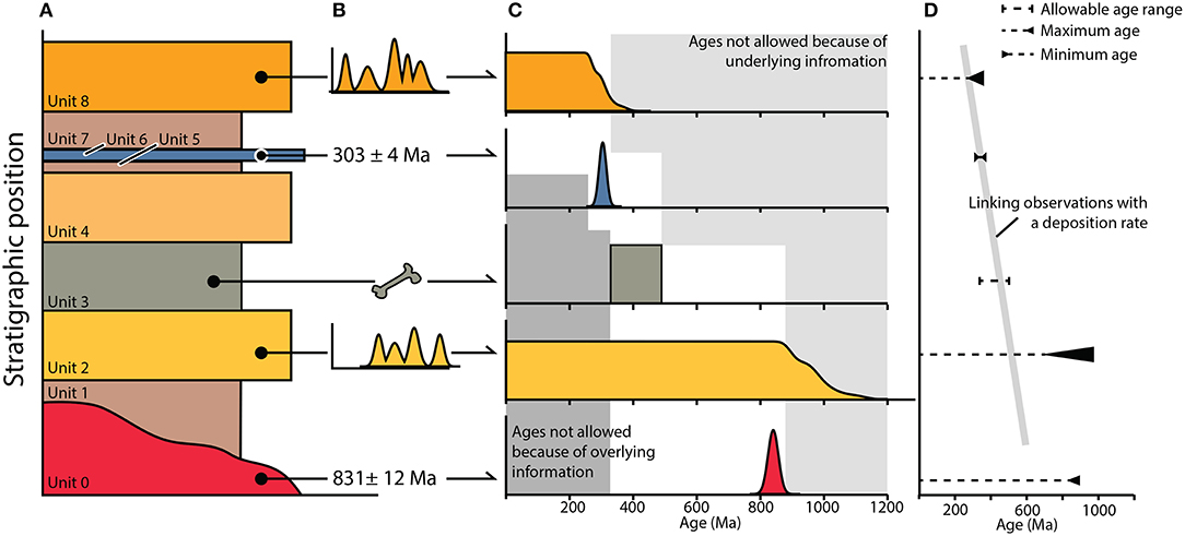
Figure 1. Cartoon illustrating the use of sets of variable observations to constrain the timing of deposition. (A) shows a stratigraphic column where a series of observations, shown in (B), were made that pertain to the ages of units within the section. (C) highlights the constraint on depositional age provided by each individual observation and the cumulative constraints provided by all observations in the section (shown in gray). In (D), all of the individual observations are linked through a curve describing a constant-rate of uninterrupted sediment accumulation.

Directly modeling the credible ages of units based on the geochronologic constraints available and their stratigraphic relationship to one another is the simplest approach conceptually. The premise of this approach (that the observed geology provides a strict relative ordering to deposits) is easily transferable to other geologic scenarios where context provides constraints on the relative age of samples (i.e., any cross-cutting relationship). Given n units in a sedimentary section that contain age information, we seek to describe the probability of the age, t_i, of the geologic unit U_i, based on a series of observations, O (Figure 1B). Here, our “observations” are those data that we collect that pertain to the age of a deposit. We refer to the probability of a set of ages for those units, t, given a set of j observations, as p(t|O), the posterior probability. Bayes rule gives:

$\begin{array}{cc}p\left(t|O\right)\propto p\left(t\right)p\left(O|t\right)=p\left(t\right){\displaystyle \prod _{i=0}^{j}p}\left(O_i|t_i\right).& (1)\end{array}$

Here, p(t) is our prior understanding of the probability of a set of n ages of stratigraphic units, information we had before collecting our observations of unit ages. The likelihood of our observations given a suite of modeled deposit ages is p(O|t), as shown in Figure 1C. Conceptually, the posterior probability of t reflects the probability of depositional ages after we have accounted for our observations. The prior probability is what we understood of the ages of units before analyzing our geochronologic data.

Some geologic units are directly dateable (e.g., ash deposits) and may result in normally distributed likelihoods (e.g., Units 0 and 6, Figure 1). Here, we consider fossil assemblages to limit the age of deposition to a range of ages (e.g., Unit 3, Figure 1) with strict bounds based on the geologic timescale (Walker et al., 2018). While this provides a useful starting point, in reality the likelihood of observing a fossil at a particular time period is not a simple step function as depicted for Unit 3 of Figure 1, as our knowledge of the timing of extinctions is not perfect and the preservation of fossils is not constant through time. We discuss the likelihood of a depositional age given a suite of detrital mineral ages more below, but the general form of the likelihood function is highlighted by Unit 2 and Unit 8 of Figure 1C: probabilities are uniform for every age we are confident is younger than the youngest grain age, and then decline according to the mean ages, uncertainties, and overlap of young grains.

The simplest way to enforce the stratigraphic ordering of our samples is the statement that a sample cannot be older than the units below it (Figure 1C) (e.g., Naylor and Smith, 1988; Bronk Ramsey, 2009),

$\begin{array}{cc}p\left(t\right)=\{\begin{array}{ll}1,\hfill & \text{if }{t}_{\text{0}}>t_{\text{1}}>t_{\text{2}}\dots t_{\text{n}-\text{1}}>t_{\text{n}}\hfill \\ 0,\hfill & \text{otherwise}.\hfill \end{array}& (2)\end{array}$

When combined with age constraints from our observations, this stratigraphic, prior constraint on the “stacking” of ages explicitly disallows those ages that would violate an age constraint from under- or overlying material (Figure 1C). It is worth noting here that we are assuming that a single point in time, t_i, can characterize the age of a deposit from which a geochronologic constraint was established and that all the dated units represent distinct events; in other words deposition of the sampled unit was instantaneous. This is a reasonable assumption when the time it takes to form a deposit is much smaller than the precision of the chronometers used to date that deposit, but shorter timescales of deposition than the millions-of-year histories we consider here and more precise dating methods require more detailed consideration of events and the constraints within them (Bronk Ramsey, 2009).

Markov-chain Monte Carlo methods (MCMC) allow us to model depositional ages according to Equation 1 given a set of observations with differing descriptions of the probability of a given age (e.g., the different shapes to the curves in Figure 1C).

Alternatively, rather than model a suite of depositional ages directly, observations throughout the stratigraphic column can be linked through a sediment accumulation rate curve (Figure 1D). Here we use the phrase “stratigraphic accumulation rate” rather than “deposition rate” because we intend to characterize the time difference between measured intervals in a stratigraphic section, which may integrate variable deposition rates, small and unrecognized unconformities, and the effects of compaction. Modeling a stratigraphic accumulation rate curve has the distinct advantage of allowing for the assessment of ages and uncertainties of depths in the stratigraphic column that are undated, but may record important events (Parnell et al., 2011). As a result, tools such as such as BChron (Haslett and Parnell, 2008; Parnell et al., 2008), OxCal (Bronk Ramsey, 2009), and Bacon (Blaauw and Christeny, 2011) have been developed to enable routine incorporation of this analysis into investigations of sedimentary successions.

As an example, consider a constant sediment accumulation rate, R [Lt⁻¹], that begins at the time of the lowest stratigraphic interval t₀; the age of unit i at the height H_i [L] above the lowest stratigraphic unit is:

$\begin{array}{cc}{H}_i=R\left(t_0-t_i\right).& (3)\end{array}$

Because H_i can be measured from the stratigraphic section, this limits the model of depositional ages to two parameters, the sediment accumulation rate, R, and the timing of initial deposition, t₀, such that $t_i=t_0-\frac{H_i}{R}$. In this framework, we modify the parameters of interest in Equation (1),

$\begin{array}{cc}p\left(t_0,R|O\right)\propto p\left(t_0,R\right)p\left(O|t_0,R\right).& (4)\end{array}$

In Equation (4), our prior probability, p(t₀, R), would be assigned so that ages decrease upsection.

The choice of a linear sediment accumulation rate is arbitrary, and it is easy to see from Figure 1 how this can cause problems. For example, a period of non-deposition between Unit 1 and Unit 0 in Figure 1A seems to best describe the observed ages of these units. It is impossible to fit a linear sediment accumulation rate through all the constraints in the column with deposition beginning at 831 Ma, the measured age of Unit 0 (Figure 1). Different forms to the sediment accumulation rate curve could be specified based on additional geologic context, and features such as unconformities could even be considered directly (e.g., Blaauw, 2010). Many existing age-depth models simulate stratigraphic accumulation rate curves in ways that allow a great deal of flexibility in the determination of accumulation rates and how they fluctuate through time (see Parnell et al., 2011, for a more detailed discussion of these approaches). For example, Bacon (Blaauw and Christeny, 2011) allows for variations in deposition rates through time as dictated by the observed age constraints (while enforcing monotonic accumulation of sediment) but can introduce smoothness to stratigraphic accumulation rate curves by simulating and assigning a prior probability to a term that governs a time period's “memory” of previous accumulation rates.

2.2. The Search for the Youngest Grain

To incorporate detrital geochronology and the Bayesian approach in our characterization of depositional ages, we must characterize the likelihood of a true depositional age given a set of detrital mineral ages (Equation 1). One of the most common methods for characterizing the formation age of the youngest mineral grains is to compute the weighted mean (and its uncertainty) of the youngest cluster of grains that overlaps within uncertainty (Dickinson and Gehrels, 2009; Coutts et al., 2019). Typically, the youngest cluster is only considered if it contains a minimum number of individual dates, k_c, where k_c is commonly three or more (Dickinson and Gehrels, 2009; Coutts et al., 2019). The theory behind this approach is that a set of overlapping ages suggests that there is a real age component present, rather than a single age being a fluke of the analysis or the result of contamination. However, a concern with this approach is that requiring a certain number of grains potentially ignores ages that are providing real depositional information, but may be fairly uncommon and therefore rarely analyzed in a given sample. A question naturally follows from this: how likely are we to actually observe k_c grains that came from the youngest unit when we date n total grains? In other words, if we require k_c grains to calculate an MDA, how likely are we to observe the true youngest age of a deposit's detrital components?

To address this, we conceptualize each of our detrital geochronometer dates as representing a lottery with one of two possible outcomes; a success or a failure. A success occurs when we date a grain from that youngest unit, a failure occurs when we do not. As was previously recognized by Andersen (2005), the question of how likely we are to identify a particular component age can be characterized as a binomial experiment. Given that the youngest geologic unit contributed a fraction of the total dateable grains deposited in a unit, f, the probability of any one date being a “success” is f and the probability of a “failure” is 1 − f. In most, if not all, ancient geologic settings, it is impossible to know what f is before conducting a detrital geochronology study. The relative contribution of detrital minerals from a young geologic source will depend on the average erosion rate, concentration of minerals of interest in that unit (i.e., its “fertility”), the areal extent of the youngest unit, and the mixing and transport of detrital sediments prior to deposition (Amidon et al., 2005). Understanding any one of these important controls on f is difficult in an ancient setting, let alone all of them. Nevertheless, we find it useful to define the quantity f as a means of exploring MDAs. The probability of dating exactly k grains from the youngest unit out of a total of n grains is given by the binomial distribution

$\begin{array}{cc}p\left(k\right)=\left(\begin{array}{c}n\\ k\end{array}\right)f^k{\left(1-f\right)}^{n-k}.& (5)\end{array}$

Here $\left(\begin{array}{c}n\\ k\end{array}\right)$ (read “n choose k”) is the binomial coefficient, which accounts for the number of ways that k “successes” and n − k “failures” could be organized in a series of n dates,

$\begin{array}{cc}\left(\begin{array}{c}n\\ k\end{array}\right)=\frac{n!}{k!(n-k)!}.& (6)\end{array}$

A more appropriate question for the purpose of determining an MDA from a detrital sample is how likely are we to undersample the youngest age population, given that we set a criterion of dating k_c grains? We can consider the odds of sampling “enough” young grains to calculate an MDA [e.g., p(k >= k_c)] by characterizing the sum of the odds of sampling too few grains. That is, if we decide we need three grains to calculate an MDA, the odds of not dating all three is the sum of the odds of dating only two grains from the youngest unit, dating one grain from the youngest unit, and dating no grains from the youngest unit. Specifically, the odds of dating enough grains for an MDA is given as one less the probability of not dating enough,

$\begin{array}{cc}p\left(k>=k_c\right)=1-{\displaystyle \sum _{i=0}^{k_c-1}\left(\begin{array}{c}n\\ i\end{array}\right)}{f}^i{\left(1-f\right)}^{n-i}.& (7)\end{array}$

If we require using at least three grains to determine an MDA, then we lower the probability that we will actually resolve the youngest MDA (e.g., Figure 2, Dickinson and Gehrels, 2009). Rather than viewing the probability field of Figure 2, we can directly ask how many grains are needed such that in 95% of cases we would date at least k_c grains from the youngest age component (Figure 3). In cases where these youngest grains make up 1% or less of all dateable minerals, we would only expect to date three of the same grains 95% of the time if we were to date around 630 grains (Figures 2 and 3). If the youngest detrital minerals only make up 1% of all dateable minerals, analyses of ~100 grains would only resolve the youngest MDA ~10% of the time. Even if we only require two dates from the same youngest unit (Figure 2, k_c = 2), it is only in cases where those youngest grains represent ~5% of all grains that we would expect to observe two of them in 95% of experiments where we dated 100 grains. While a simplification, Equation (5) reflects results from previous work that large numbers of analyses are essential for confidently resolving the youngest population of grains through repeated analyses (e.g., Coutts et al., 2019).

FIGURE 2

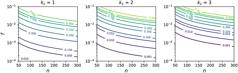
Figure 2. Probabilities of dating enough grains from the youngest constituent to compute an MDA, given that k_c grains are required to compute an MDA and that the grains belonging to the youngest age component constituents a fraction f of all dateable grains (Equation 7). The three panels show probability contours for k_c = 2, 3, and 4.

FIGURE 3

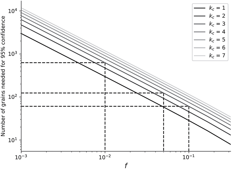
Figure 3. How many grains should be dated in order to be 95% confident that we would date at least k_c grains from the youngest source of grains? The solid lines provide this recommendation as a function of f, the fraction of dateable mineral grains from the youngest source. In practice, it is unlikely that this quantity can be known. The dashed lines represent specific recommendations for if f = 10, 5, and 1%. In 95% of cases where you date 50, 90, and 500 grains, at least 3 grains will be dated from sources that contributed 10, 5, and 1% of all the dateable minerals.

Equation (5) and Figure 2 highlight another concern with methods that seek to quantify an MDA through averaging replicate measurements and assigning an uncertainty to the resulting MDA: that the resulting uncertainty is not a actually a measure of confidence in the MDA, but rather a measure of the similarity and precision of those ages that were selected as representative. In other words, the 2σ bound on pooled MDA methods does not reflect 95% confidence in the youngest grains in a population being drawn from that interval, because we may have had a very small chance of observing the youngest grains to begin with (Figure 2).

2.3. Transforming Maximum Depositional Ages Into Predictions of True Depositional Age

It is challenging, if not impossible, to identify an infallible method to compute a single MDA from a series of ages; how can you appropriately characterize confidence in establishing the age of the youngest material when it is impossible to know how common that material should be (e.g., f of Figure 2)? How likely is it that your sample was contaminated or that a mineral grain retained, and you measured, all of its parent and daughter isotopes?

To compute MDAs we rely on an approach presented by Keller et al. (2018). We model the timing of last crystallization as the truncation of a prior expectation of the probability of zircon ages. Given a prior understanding of the relative proportions of dateable grains formed throughout mineral growth, f_xtal, we can modify that distribution by truncating the probability of observing an age, t_obs, greater than the time at which the first mineral crystallized, t_sat, and less than the time at which the youngest crystal could have formed, t_e,

$\begin{array}{cc}p\left(t_{obs}|t_e,t_{sat}\right)=\{\begin{array}{ll}0,\hfill & \text{if }{t}_{obs}<t_e\hfill \\ 0,\hfill & \text{if }{t}_{obs}>t_{sat}\hfill \\ f_{xtal}/\left(t_{sat}-t_e\right),\hfill & \text{otherwise.}\hfill \end{array}& (8)\end{array}$

Keller et al. (2018) present results constructing f_xtal from expectations derived from a thermodynamic model of a steadily cooling magma body, from kernel density estimates derived from observed ages within the dated unit, and with a uniform prior that makes no assumptions about the relative timing of crystallization (e.g., f_xtal = 1 in Equation 8). Here, we utilize the uniform prior approach, as detrital distributions likely integrate complex histories of crystal growth and recycling which we don't presume to be able to fully characterize. We utilize a Markov-Chain Monte Carlo Model (Foreman-Mackey et al., 2013) to infer the posterior distributions of t_e and t_sat, although for MDA analysis we are only interested in the former. In this approach, a series of “walkers” take random steps about an initial guess of parameters such that they first explore the parameter space (a “burn-in” phase) and then take steps such that the frequency of parameters sampled at each step mirrors the posterior probability of those parameters. From initial guesses of t_e and t_sat that vary randomly about the youngest and oldest ages in a sample, respectively, we update these estimates over 700 steps taken by an ensemble sampler with 100 walkers and trim a burn-in period of 200 steps from the sample-chain constructed by each walker, resulting in 50,000 samples characterizing the posterior of t_e and t_sat.

Examples of MDAs calculated with the weighted mean of the youngest grain cluster overlapping at 2 sigma (YGC2σ, Dickinson and Gehrels, 2009) and t_e estimates are shown in Figures 4D,F. In the example shown in Figure 4D, there is relatively good agreement between the two samples, as an isolated cluster of three young grains defines the MDA calculated with the YGC2σ method. However, the example shown in Figure 4F shows how the two methods can deviate; an over-dispersed but overlapping cluster of grains pulls the YGC2σ MDA toward older values, while t_e is limited by the youngest observed grains. Unlike the weighted mean approach, characterizing t_e does not require the selection of a sub-population of observed ages and is therefore able to produce reliable estimates without interpretations of groupings. For these reasons, in addition to those discussed in Keller et al. (2018), we use t_e to characterize MDAs from here out in the text.

FIGURE 4

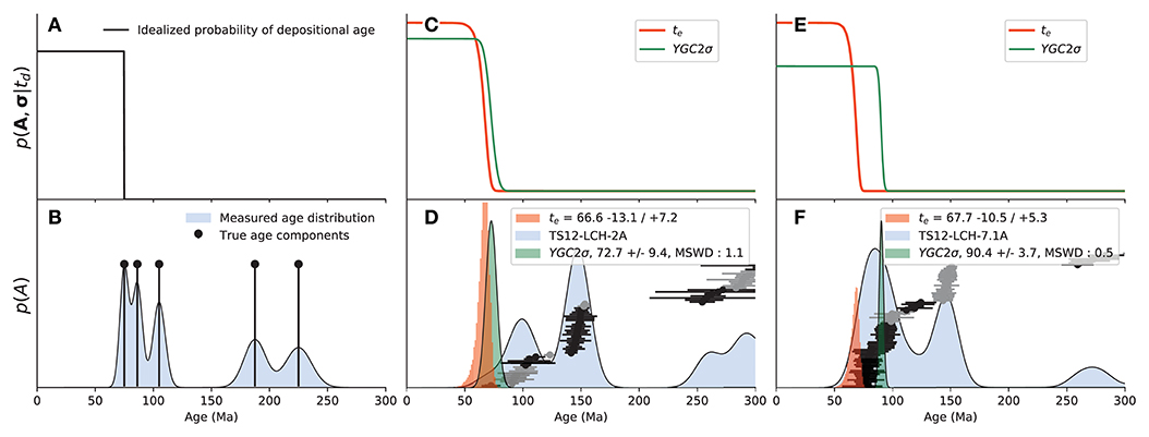
Figure 4. The top row highlights probabilities of observing a set of detrital ages (A),σ, given an age of the deposit t_d, whereas the bottom row shows our observations. (A,B) show an idealized example, where we have absolute confidence that we have characterized the true formation age of constituent minerals, shown in (B), so that the deposit is equally likely to be any age younger than the youngest age component. (B) also highlights an example of how we might have characterized the distribution of ages of this example based on measurements. (D,F) highlight real detrital zircon geochronology data, whereas (C,E) show example likelihood functions for the depositional age of these samples based on two methods for determining MDAs from observed data. In (D,F), a Gaussian kernel density estimate with a 10 Ma bandwidth (Vermeesch, 2012) is shown alongside the observed ages and their uncertainties (shown as circles with lines showing the 95% confidence intervals). Individual ages are shown in alternating colors to indicate different groups. Groups are defined based on overlap of the 2σ confidence interval of the youngest grain in that group.

More important than the MDA method used is the recognition that when using detrital geochronology data to understand geologic histories, it is the true depositional age that we are typically interested in. The bottom row of Figure 4 highlights the probabilities of crystallization ages. The top row of Figure 4 highlights our focus in the manuscript, how likely is it that we would have observed a suite of detrital mineral ages if the deposit were of a certain age? We refer to this as p(A, σ|t_d), the likelihood of a series of ages, A, and their associated uncertainties, σ, given a depositional age t_d. If we knew the true age components of our sample (Figure 4B), then p(A, σ|t_d) would be equal for all ages younger than the youngest true component age (Figure 4A), but there is no chance (e.g., p = 0) that one of these true component ages could be less than t_d. In some situations, for example known proximity to an active arc, future work may wish to consider the situation where true depositional ages close to those of the youngest zircons are more likely than those associated with large lags between crystallization and deposition. We ignore this special case and just consider detrital ages to define upper bounding ages. Our characterization of the youngest mineral ages is subject to uncertainties associated with our measurements and our ability to identify the youngest mineral ages from within a complex population (Figures 4C–F). Here we assume that we can characterize the likelihood of observing a set of detrital mineral ages given a true depositional age, p(A, σ|t_d), based entirely on the probability that the depositional age is less than the MDA,

$\begin{array}{cc}p\left(A,\sigma |t_d\right)=\frac{1-{\displaystyle {\int }_0^{t_d}p}\left(t|MDA\right)dt}{{\displaystyle {\int }_0^{4.5Ga}1}-p\left(t|MDA\right)dt}.& (9)\end{array}$

Here, p(t|MDA) refers to the probability of a particular age, t, characterizing an MDA. In the case of YGC2σ this would be governed by a normal distribution, but the probabilities of t_e are not necessarily normally distributed. The numerator in Equation 9 is just a mirror image of the cumulative density function of the MDA (Figures 4A,C,E). The denominator in Equation 9 integrates over the age of the earth to ensure that the probabilities of all possible ages integrate to one. Plotting Equation (9) emphasizes that these are indeed only maximum depositional ages; providing no information about the lower bound on possible depositional ages (Figures 4C, E). It is only through context with other neighboring samples that we can determine bound estimates of true depositional ages.

2.4. Examples of Depositional Age and Uncertainty Inference

We use synthetic examples to demonstrate how the depositional ages inferred using Equation (1) respond given ideal and, perhaps, more common scenarios with detrital geochronology. Figure 5 highlights a stratigraphic section from which five geochronology samples were collected. The lower four are all detrital geochronology samples, while the upper sample is a direct date of an ash bed (this sample provides a lower-limit to the underlying ages). Figure 5B highlights a well-behaved example; the best-case scenario where the youngest grains from a suite of detrital geochronology samples nearly overlap or young upsection and are close to overlapping with the absolute age constraint at the top of the section (Figure 5B). Figures 5C,D provide increasingly complicated scenarios: in Figure 5C not all youngest grain ages decrease upsection, and in Figure 5D there is a large time gap between the youngest grains of the basal sample and the second sample up from the bottom of the section. The examples shown in Figures 5C,D are derived by incrementing all the observed ages in a subset of samples shown in Figure 5B.

FIGURE 5

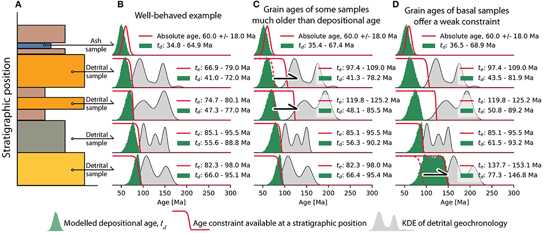
Figure 5. A synthetic example of a stratigraphic section (A) with five geochronologic constraints. The bottom four age constraints are from detrital geochronology samples, the top sample represents a dated ash bed (or any other deposit that can be directly dated). The plot in column (B) is an idealized example; plots in columns (C,D) are results given modifications to (B). In (B-D) each row shows the posterior probability of the depositional age of that unit as a green histogram of MCMC samples with 50 evenly spaced bins, the likelihood of a depositional age given the data available for that deposit, and for detrital geochronology sample a KDE constructed with a gaussian kernel with a bandwidth equal to the mean 2σ uncertainty of samples. The black arrows in (C,D) show the datasets that were perturbed from the case shown in (B). In each plot of model results, the legend indicates the 95% credible interval for the modeled true depositional age t_d and, for detrital geochronology samples, the MDA, t_e, determined with the approach of Keller et al. (2018).

To integrate the individual age constraints informed by observations within individual deposits (e.g., the detrital geochronology data and age of the upper ash that inform the likelihood of a unit's age, p(O|t) of Equation 1) with the constraints dictated by stratigraphic ordering (Equation 2), we utilize a Monte Carlo sampling approach. We make a guess of the age for each sample and then evaluate both its prior (Equation 2) and likelihood (e.g., Equation 1, Figure 7). Specifically, we employ a Bayesian, MCMC approach with an affine-invariant ensemble sampler (Foreman-Mackey et al., 2013). In each iteration, a series of “walkers” (each walker makes parameter guesses and evaluates them) takes a “step” by evaluating a suite of parameters (e.g., the vector of true depositional ages t). In the MCMC approach, the suite of guessed ages is chosen such that over time, the frequency with which ages are sampled mirrors the posterior probability (Foreman-Mackey et al., 2013; VanderPlas, 2014). For detrital samples, we first model the posterior of t_e and use this to numerically evaluate (Equation 9). For this work, we ignore all grain ages older than 200 Ma in MCMC models of t_e. We run the MCMC models of t_d with 200 walkers that each take a total of 1,200 steps, and we trim the first 400 steps from each walker to allow for a ‘burn-in’ phase of the model where the sampler explores the parameter space around the initial guesses. Because of the stiff constraints imposed by stratigraphic ordering, we find that having a large number of samples characterizing the burn-in phase can be necessary to allow the model to fully explore the parameter space. Although we do not explore this concept here to maintain simplicity, the true depositional age also limits t_e, providing additional prior information that could be exploited if one simultaneously modeled values of t_e and t_d in a stratigraphic succession.

In the well-behaved example of Figure 5B, we are able to predict comparable uncertainties (a 95% credible interval of 30 Ma) for all samples despite only having a single absolute age constraint. The other way of viewing this, is that we are able to propagate the confidence we have from the directly dated sample into predictions of true depositional ages lower in the section.

Having some samples that do not contain MDAs close to the true depositional age does not necessarily substantively impact our predicted depositional ages (Figure 5C). While the top two detrital samples in Figure 5C have much older youngest grains than those in Figure 5B, the predicted true depositional ages for these samples are only marginally older in example C. This is because the upper samples did not provide much information that was not already available from one of the lowermost two samples due to the overlap in t_e within these deposits (Figure 5).

In Figure 5D, the ages of the youngest grains in the basal sample are much older than the youngest grains in the next sample upsection. This results in a broad, flat-topped posterior probability of true depositional ages because there is an extensive region between where overlying samples provide information limiting the youngest ages and the grains provided in this sample limit the oldest allowable age. The change in ages of the basal sample also impacts the credible intervals of ages in all the overlying samples (allowing the upper bounds of most samples to increase by 4 Ma). This is reflecting the complex covariances that exist between the modeled true depositional ages of samples, and the cascade of information that propagates through the prior constraint of superposition. If the upper bounding absolute constraint was not present (and there were no other constraints available to provide minimum bounds on ages), then all the modeled posterior probabilities of true depositional ages would be broad plateaus, similar to that in the bottom sample of Figure 5D, but extending all the way to the present.

The other phenomenon highlighted by the examples in Figure 5 is how detrital geochronology can refine the age estimates provided by direct dating. The uppermost age in these examples has a broad uncertainty, but in Figure 5B, the median value inferred from the depositional age model (t_d) is shifted to be younger than the mean age of the absolute date. In Figure 5B, the underlying detrital geochronology samples provide information that shifts this sample to younger values, but as the constraints provided by detrital geochronology are relaxed (in Figures 5C,D), the posterior estimate of t_d from the depositional age model becomes closer to the assigned absolute age.

3. Application to the Magallanes Basin, Patagonia

3.1. Geologic Setting and Data Exposition

The Magallanes basin is a retroarc foreland basin that formed during Late Cretaceous to Neogene uplift of the southern Andes (Wilson, 1991). The foreland basin is floored by attenuated, transitional-oceanic crust associated with the Jurassic-Early Cretaceous Rocas Verdes extensional basin (Dalziel et al., 1974; Dalziel, 1981; Biddle et al., 1986; Wilson, 1991). Loading and flexure of the dense, attenuated crust facilitated the formation of a deep-marine foredeep (Natland, 1974; Fosdick et al., 2014), which accumulated more than 4 km of deep-marine basin floor to slope deposits (Punta Barrosa, Cerro Toro, and Tres Pasos Formations; Biddle et al., 1986; Romans et al., 2010; Fosdick et al., 2011) that are overlain by up to 1 km of shelfal deposits (Dorotea Formation; Schwartz and Graham, 2015) during Late Cretaceous time (Figure 6). The uppermost deep-marine deposits (Tres Pasos Formation; Figure 6) and overlying shelfal deposits (Dorotea Formation; Figure 6) record shoaling in the foredeep between ca. 80–65 Ma, and together represent a genetically linked shelf and slope that prograded southward along the axis of the Magallanes foredeep (Macellari et al., 1989; Covault et al., 2009; Hubbard et al., 2010; Schwartz and Graham, 2015; Schwartz et al., 2017; Daniels et al., 2018a).

As a whole, the Magallanes foreland basin fill is well-constrained based on lithostratigraphic correlations, radiometric dates from ashes, and MDAs from detrital zircon samples (Fildani and Hessler, 2005; Romans et al., 2010; Bernhardt et al., 2011; Fosdick et al., 2011; Malkowski et al., 2017; Schwartz et al., 2017; Daniels et al., 2018a). Ashes are relatively abundant in the deep-marine phase of the basin fill (e.g., Fildani and Hessler, 2005; Bernhardt et al., 2011; Fosdick et al., 2011; Malkowski et al., 2017), but have not been observed above the base of the Tres Pasos Formation (Schwartz et al., 2017; Daniels et al., 2018a). Detrital zircon MDAs in the deep-marine section have been shown to closely overlap with stratigraphically adjacent ash ages (Bernhardt et al., 2011; Malkowski et al., 2017), supporting connectivity between the active Patagonian arc and foredeep as well as rapid transfer of volcanogenic sediment from the arc to the retroarc foreland basin (Schwartz et al., 2017). In addition, most detrital zircon MDAs from the shallow-marine section exhibit apparent younging up-section, supporting continued connectivity between the arc and foredeep through time and suggesting that MDAs may closely track true depositional ages of the deposits (Schwartz et al., 2017; Daniels et al., 2018a). In addition to radiometric age constraints, the Dorotea Formation contains relatively abundant fossil assemblages including ammonites, bivalves, shark teeth, and dinosaurs (Schwartz et al., 2017).

Lithostratigraphically, we simplify the 2.25 km-thick Tres Pasos-Dorotea depositional system into three conformable lithofacies assemblages: (1) mudstone-dominated slope clinoforms of the Tres Pasos Formation (1,200 m thick) that downlap onto basinfloor deposits of the Cerro Toro Formation; (2) sandstone-dominated delta-front clinoforms of the Dorotea Formation (300 m thick) that interfinger with topsets of the Tres Pasos Formation; and 3) heterolithic delta-plain deposits of the Dorotea Formation (750 m thick, Figure 6, Schwartz et al., 2017). Figure 6 shows the vertical distribution of twenty existing age constraints for the Tres Pasos-Dorotea succession (compiled from Schwartz et al., 2017; Daniels et al., 2018a): (1) one ash at the base of the Tres Pasos Formation; (2) fourteen detrital zircon samples that are distributed throughout the Tres Pasos and Dorotea formations, one of which (TS12-LCH-7.1A) is interpreted as a fluvially reworked ash; and (3) five fossil assemblages from the Dorotea Formation (Figure 6, Table 1).

FIGURE 6

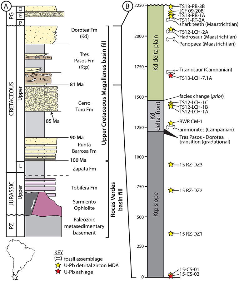
Figure 6. Stratigraphic context for the zircon data modeled in this paper. (A) Simplified stratigraphic column for the Rocas Verdes and Magallanes basin fill in southern Chile, between approximately 51° 30' S and 50° 30' S (modified from Fosdick et al., 2011; Schwartz et al., 2017; Daniels et al., 2018a,b). Numeric ages in bold indicate well-established radiometric ages for major lithostratigraphic boundaries in the basin fill (after Daniels et al., 2018a,b). (B) Highly simplified, composite stratigraphic column for the Tres Pasos and Dorotea Formations at approximately 50° 45' S, which record shoaling in the Magallanes foredeep from bathyal to non-marine environments through the successive deposition of progradational slope, delta-front and delta-plain deposits (after Schwartz et al., 2017; Daniels et al., 2018a). The stratigraphic positions of all available ash, detrital zircon, and fossil age constraints are indicated to the right of the column.

TABLE 1

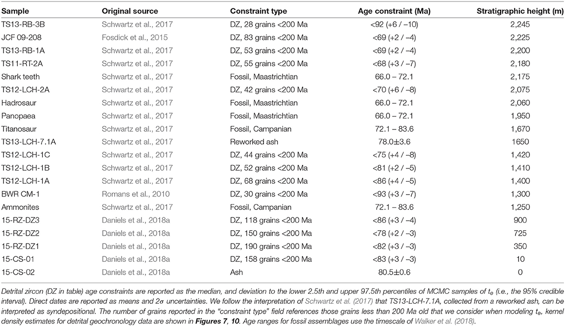
Table 1. Summary of data sources and ages constraints used in modeling depositional ages of the Magallanes-Austral Basin.

The Tres Pasos-Dorotea succession provides a unique opportunity to test our proposed modeling framework for depositional ages for two reasons. First, this example includes abundant and varied age constraints that are relatively evenly distributed throughout the > 2 km succession of strata, but a relatively limited number of them (2 of 20) are expected to directly record the timing of deposition. As a result, we can explore how well the modeling framework can refine estimates of the timing of deposition provided by different sets of observations. Second, detailed sedimentological comprehension of the Tres Pasos-Dorotea depositional system provides confidence in the relative stratigraphic position of various age constraints and in the depositional environment, from which we can construct an informed expectation for the form of a sedimentation rate curve. In the two sections that follow, we explore how both the constraints of stratigraphic ordering (Equation 2, Figure 1C) and a sediment accumulation rate curve (Figure 1D) refine our models of depositional ages based on geochronology data. For all detrital zircon geochronology samples we recompute an MDA (following Keller et al., 2018, see above) independent of modeling t_d, but for samples where direct age constraints are available we describe the likelihood of depositional ages using the reported ages and uncertainties of the presenting studies rather than reanalyzing the data ourselves (Table 1).

3.2. Modeling the Ages of Stratigraphy With Stratigraphic Ordering

We begin by investigating the impacts of enforcing stratigraphic ordering (Equation 2) on the modeled depositional ages of the lower approximately 1,500 m of the Tres Pasos-Dorotea succession (Tres Pasos slope clinoforms through Dorotea delta-front clinoforms, samples 15-CS-02 through the Titanosaur observation above TS12-LCH-7.1A; Figure 6). This lower part of the Tres Pasos-Dorotea succession is bracketed by absolute age constraints. At the base, sample 15-CS-02 is an ash with 13 zircons dated by isotope dilution-thermal ionization mass spectrometry (ID-TIMS, Daniels et al., 2018a). At the top, sample TS12-LCH-7.1A is a detrital sample with 99 zircons dated by LA-ICP-MS (Schwartz et al., 2017). Based on the sedimentological characteristics of the sampled bed, its modal composition, and the presence of 21 zircon grains defining an indistinguishable, young population, Schwartz et al. (2017) interpreted this unit to be a fluvially reworked ash. We follow the interpretation of Schwartz et al. (2017) and assume that the youngest grain ages in this deposit are syndepositional, such that their age characterizes the true depositional age (i.e., although it is a detrital sample, it is treated as an ash). In the middle of this sub-section, at the transition from Tres Pasos slope clinoforms to Dorotea delta-front clinoforms, an ammonite fossil assemblage restricts the timing of deposition to Campanian (72.1 - 83.6 Ma; age bounds after Walker et al., 2018). A Titanosaur fossil at the top of this sub-section further restricts deposition to within the Campanian. Based on these fossil assemblages, we treat the likelihood of an age of this unit (Equation 1), that is the probability of the observation of this fossil assemblage given an age for the unit, as equally likely within the range 72.1–83.6 Ma and impossible outside this range (Figure 7). As discussed above, this likelihood is in no doubt an oversimplification, but nonetheless provides a starting point for incorporating these data. Within this lower interval, eight other detrital zircon samples provide additional age constraints (Figure 7). We describe the likelihood of a true depositional age at the stratigraphic height associated with each of these detrital samples with Equation (9). We refer to the modeled ages of this stratigraphy later in the text as the “well constrained” age only model.

FIGURE 7

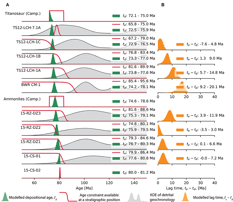
Figure 7. Results of modeling the ages of stratigraphic units from the lower half of the study section (Figure 6). Each row shows one of the stratigraphic units that contains an age constraint. Age constraints and modeled ages are shown in column (A). In (A), each row shows a KDE constructed with a gaussian kernel with a bandwidth equal to the mean 2σ uncertainty of samples if that row corresponds to a detrital geochronology sample, the likelihood of a depositional age given the data available for that deposit as a red line, and the posterior probability of the depositional age of that unit as a green histogram of MCMC samples with 50 evenly spaced bins. In each plot, the legend indicates the 95% credible interval for the modeled true depositional age t_d and, for detrital geochronology samples, the MDA, t_e, determined with the approach of Keller et al. (2018). For those samples where we compute t_e, column (B) highlights the duration between the modeled timing of last crystallization (t_e) and the modeled timing of deposition (t_d), refered to here as ‘lag time’ (Brandon and Vance, 1992; Romans et al., 2016).

We initialize the model with random parameter guesses that obey stratigraphic ordering and are within the intervals allowed by overlying, underlying, and local information (e.g., within the interval bound by the gray regions in Figure 1). From our initial estimates, we run the MCMC model for 4,000 iterations after an initial burn-in period of 1,000 iterations with 300 walkers. Examination of the results with these parameters shows that this number of iterations allows the model to explore the allowable parameter space during the burn-in phase of the model, so that the post burn-in iterations reflect a stable sampling of the posterior distribution.

3.2.1. Results and Discussion

Histograms of the MCMC samples for the depositional ages model after the burn-in period, which approximate the posterior probabilities of depositional ages, are shown in Figure 7A. We summarize the MCMC samples for each depositional age (t_d) and MDA (t_e) with the 95% credible interval approximated by the MCMC samples. The modeled ages for all units are limited to fairly precise ranges (95% credible intervals span ~3-4 Ma) despite limited absolute age constraints. As was highlighted by Figures 5C,D, this is a function of the strong age constraints that are available within this section. At the base of the section, the high-precision ID-TIMS date (Daniels et al., 2018a) provides a narrow range of allowable ages, and the identified fossil assemblages (Schwartz et al., 2017) provide lower limits to depositional ages close to the MDAs.

Even though modeled MDAs do not get consistently younger up-section (Figure 7A), our stratigraphic constraint (Equation 2) enforces this behavior in the modeled true depositional ages. This is highlighted by directly computing a posterior probability distribution on the “lag-time” between the time of last zircon crystallization and the timing of deposition in the unit of interest (ignoring that in some instances those youngest zircons could have been recycled from other sedimentary units) (Brandon and Vance, 1992; Romans et al., 2016). We compute distributions of lag-time by differencing the MCMC sampled distributions of t_e and t_d (an approach similar to Kruschke, 2013). The lower three detrital zircon samples have lag-times of a few million years or less, but lag-time increases substantially for sample BWR CM-1 (to greater than 10 Ma), and then decreases again toward a few million years or less moving up in the section (Figure 7B).

The computed 95% credible intervals of lag time include and extend beyond zero in samples TS12-LCH-1C and 15-RZ-DZ2. Negative lag-times are not possible. The presence of negative lag-times here reflects that we compute our MDA and t_d independently of one another, and that the uncertainty in the independently calibrated MDA allows for overlap with the modeled true depositional age. In other words, these models suggest nearly synchronous crystallization and deposition of the youngest grains in these samples, but uncertainty in measured ages can results in some dated grains whose age are less than the depositional age (Coutts et al., 2019).

3.3. Modeling the Accumulation of Sediment as a Prograding Shelf-Slope System

Previous sedimentology-based studies have interpreted the Tres Pasos and Dorotea Formations to record a transition from marine to terrestrial environments, represented by progressive shoaling of slope and shelf deposits (Macellari et al., 1989; Covault et al., 2009; Hubbard et al., 2010; Schwartz and Graham, 2015; Schwartz et al., 2017). Here, we use this field-based interpretation to establish further constraints on the history of deposition by modeling the depositional ages of stratigraphy in the context of a stratigraphic accumulation rate (e.g., Figure 1D). In light of these interpretations, we attempt to describe the depositional history with a simple model of the stratigraphic accumulation rate expected for a steadily prograding shelf-slope system (Figure 8A). Specifically, we model a change in accumulation rate that may be expected to occur with the transition from deposition on the continental slope recorded by the lower portion of the section, to deposition on the shelf recorded by the upper portion of the section (e.g., Carvajal and Steel, 2009; Schwartz et al., 2017). Consider a stratigraphic succession being deposited at the 0 coordinate of the x-axis in Figure 8A. As the simplified and idealized shelf-slope system progrades self-similarly out into the basin and over this point, indicated by the star, aggradation will first occur quickly due to the steep gradient of the slope, and will then slow once that point is overtaken by the prograding shelf (at which point we would also expect a change in depositional environment). We simplify this depositional history by expressing this progradation with two stratigraphic accumulation rates, R₀ and R₁, which respectively represent deposition on the slope and shelf,

FIGURE 8

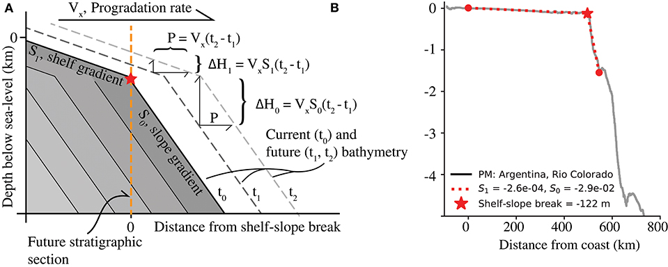
Figure 8. Conceptual model of the accumulation of the Tres Pasos and Dorotea Formations in the Magallanes basin. (A) schematically depicts the accumulation of strata as the result of a prograding shelf-slope system that is advancing self-similarly through time. In this model, the local magnitude of aggradation ΔH is related to the local progradation P by the gradient of the depositional system. As a result, we expect a decrease in vertical sediment accumulation rates (R) when crossing from the higher-gradient shelf to the lower-gradient slope. (B) depicts the bathymetric profile of a modern shelf-slope system (offshore of Rio Colorado, Argentina; PM - passive margin) measured from ETOPO1 elevations data (Amante and Eakins, 2009) and highlights our method for aggregating topographic data from modern systems. The thin, gray line is the entire profile we collected, from which we only consider those elevations below sea-level and above 1,000 m water depth. The thin dashed lines depict the fitted topographic profile, from which we calculate S₁ and S₀, with the shelf-slope break identified by the star.

$\begin{array}{cc}H\left(t\right)=\{\begin{array}{ll}H=R_0\left(t-t_0\right),\hfill & \text{if }H<H_c\hfill \\ H=H_c+R_1\left(t-t_c\right),\hfill & \text{otherwise}.\hfill \end{array}& (10)\end{array}$

Here, H_c is the height in the stratigraphic section where deposition rates slow from R₀ to R₁, which is derived based on the time that deposition on the continental shelf begins, t_c,

$\begin{array}{cc}{H}_c\text{ = }{R}_0\left(t_c\text{ - }{t}_{\text{0}}\right)\text{.}& (11)\end{array}$

Given steady, self-similar progradation of a shelf-slope system (Figure 8), the rates R₀ and R₁ can be considered to be the product of the local depositional gradients, S, and the progradation rate, V_x,

$\begin{array}{cc}{R}_0=V_x{S}_0,R_1=V_x{S}_1.& (12)\end{array}$

From this, we see that we would expect the ratio of accumulation rates to be equivalent to the ratio of depositional gradients on the shelf, S₁, and slope, S₀,:

$\begin{array}{cc}\frac{R_0}{R_1}=\frac{V_x{S}_0}{V_x{S}_1}=\frac{S_0}{S_1}& (13)\end{array}$

While we may have little prior knowledge regarding the deposition rates in the Magallanes basin, if that depositional system was similar to those on earth today, we can make a good prediction of $\frac{S_0}{S_1}$ based on the ratio of depositional gradients observed in modern shelf-slope systems. If the assumptions made in deriving (Equation 13) are valid, then the ratio of modern shelf-slope gradients (Figure 8B) can provide insight into how much accumulation rates may have changed when transitioning from deposition on the slope to deposition on the shelf. We can insert this expectation into our model of stratigraphic accumulation rates in the form of a statement about prior probability in Bayes' rule (Equation 1).

To develop our expectation of $\frac{S_0}{S_1}$, we compiled 45 bathymetric profiles across modern shelf-slope breaks from ETOPO1 elevation data (Amante and Eakins, 2009) using Google Earth Engine (Gorelick et al., 2016). Profiles were selected in order to provide an adequate representation of the variation in shelf-slope morphologies using the following criteria: (1) all profiles were collected from siliciclastic-dominated systems (i.e., excluding high-relief carbonate banks, etc.); (2) the set of profiles is affected by a spectrum of wave-, tide-, and river-associated processes, but with a preference for fluvial input at the shoreline to mimic the Magallanes basin example; (3) all profiles extend across the entire shelf, include the shelf-slope break, and end at the approximate base-of-slope; and (4) no profiles cross plate boundaries, but may be closely associated with one. Between sea-level and depths of 1,500 m, we fit a piece-wise linear-regression by minimizing the sum of the squared errors between that fitted surface and the topography (Figure 8B). This regression intends to mimic a simple slope break where the average bathymetric gradient transitions from shallow to steep, a kinked topographic surface representing a simplified shelf-slope geometry (Figure 8). All extracted topographic profiles are shown in Figure 9A, with their best-fitting counterparts shown in Figure 9B. In these plots we stack all the data so that 0 on the x- and y-axes is at the shelf-slope break.

FIGURE 9

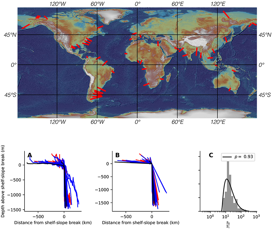
Figure 9. Compilation of observations from 45 modern shelf-slope systems. Map of shaded relief topography from ETOPO1 elevation data (Amante and Eakins, 2009) shows the locations of extracted bathymetric profiles in red. The bottom row (A–C) shows the data extracted from the profiles. (A) is a composite of all profiles of bathymetry collected from ETOPO1 elevation data (Amante and Eakins, 2009), hung so that 0,0 is at the best fit shelf-slope break. (B) depicts all of the simplified topographic fits for the profiles. In (A,B), red, blue, and black lines indicate profiles from convergent, passive, and rifted margins, respectively. (C) depicts the ratio of slope to shelf gradients (e.g., Equation 13), with the thin black line indicating the best fitting distribution of relative gradients of the slope and shelf. Under the assumption that progradation of a similar system was steady, and occurred self-similarly, we use this distribution to characterize the prior probability on the ratio of accumulation rates on the slope and shelf, $\frac{R_0}{R_1}$. The K-S test does not reject the null hypothesis that the observations of shelf-slope data were drawn from this distribution (p = 0.93).

The ratio of shelf to slope gradients, $\frac{S_0}{S_1}$ (Figures 8, 9C), is well-described by a log-normal distribution with a shape σ_R = 1.2, location, θ_R = 5.3, and scale, m_R = 29.4, so we take this as the prior probability of the ratio of accumulation rates ($\frac{R_0}{R_1}$),

$\begin{array}{cc}P\left(R_0,R_1\right)=\frac{1}{(\frac{R_0}{R_1}-{\theta }_R){\sigma }_r\sqrt{2\pi }}{e}^{\frac{-ln{\left(\right(\frac{R_0}{R_1}-{\theta }_R)/m_r)}^2}{2{\sigma }_R^2}}.& (14)\end{array}$

From stratigraphic observations we also have expectations of where in the section we expect stratigraphic accumulation rates to transition from R₀ to R₁ (that is, the stratigraphic height, H_c in Equation 10). There is a lithofacies transition between Dorotea delta-front clinoforms and Dorotea delta plain deposits at approximately 1,450 m in the examined section (after Schwartz et al., 2017). Since the Dorotea delta-front was attached to the shelf-edge (i.e., a shelf-edge delta) (Schwartz and Graham, 2015; Schwartz et al., 2017), the lithofacies transition from delta-front to delta-plain can effectively be considered to represent a change from slope-dominant deposition to shelf-dominant deposition. Defining a continuous prior probability on H_c is more challenging than it was for $\frac{R_0}{R_1}$, where that probability function was dictated by a large number of observations.

The transition in lithofacies used to define H_c at 1450 m occurs within an approximately 150 m-thick succession of sandstone and conglomerate that represents tidally influenced mouth bars and distributary channels (e.g., facies assemblage 3 after Schwartz et al., 2017). We select the parameters of a t distribution describing H_c to conservatively match the scale of this lithofacies unit (Schwartz et al., 2017). Specifically, this is done so that the 95% confidence interval ranges 100 m on either side of 1450 m transition (encompassing the majority of the delta-front interval) and that the 99% confidence bounds extend an additional 150 m beyond this (extending an additional thickness of this lithofacies beyond the 95% interval). This is accomplished with a t distribution with a location, μ of 1450, a scale, σ of 25, and a value, v of 2. We utilize a t distribution to describe our prior probability on H_c because the broad tails allow us to acknowledge that this identification was subjective and that the model should be able to explore values well-outside of our assigned central value. Although v typically denotes the degrees of freedom, we instead use it here as a “normality” parameter (Kruschke, 2013); smaller values of v expand the tails of this distribution and cause it to deviate from a normal distribution.

From our initial estimates, we run the MCMC model for 5,000 iterations after an initial burn-in period of 500 iterations with 400 walkers. We use a starting guess of t₀ = 79.5, of R₀&R₁ = –1,000 & –95 and t₁ = 78.0, as these are consistent with our priors and able to predict ages for all deposits with temporal constraints. The negative values of R indicate that strata accumulate as ages decrease. We start each walker with initial guesses drawn from a normal distribution with the previously mentioned means and a 0.1% relative error. From these initial guesses the MCMC model is able to expand to a stable sampling space over the burn-in period.

3.3.1. Results and Discussion

Results for the model of stratigraphic accumulation rates are shown in Figure 10, which highlights both the modeled depositional ages and the modeled stratigraphic accumulation rate curve from which these ages are derived. For each age, we report the 95% credible interval derived from the MCMC samples. All of the geochronologic constraints can be appropriately described by a ‘kinked’ stratigraphic accumulation rate that transitions from a relatively rapid accumulation rate to a slower one at H_c = 1456 (+100, –104) m (reported as the median and the range between the 5th and 95th percentiles of the MCMC samples characterizing the posterior), approximately the position of a change in depositional facies (Figures 6, 10). The lower, more rapid sediment accumulation rate R₀ = –675 (–1031, +227) m/Ma, we associate with progradation of the Tres Pasos slope. The slower accumulation rate in the upper part of the section, R₁ = –65 (–14, +11) m/Ma, we associate with the Dorotea delta-plain (Figure 6). Based on the relative gradients in modern systems $\frac{S_0}{S_1}$ (Figure 9), we expect the ratio of accumulation rates in self-similarly propagating shelf-slope systems, $\frac{R_0}{R_1}$, to be 11.7. This is similar to the median posterior value of 10.3 observed from our model of the Magallanes basin. In summary, the available geochronologic data are not sufficient to provide a substantive update of our prior knowledge of H_c, resulting in a nearly identical posterior. Similarly, there is much overlap between the prior and posterior distributions on relative rates $\frac{R_0}{R_1}$, but the posterior distribution indicates a much lower probability of relative rates greater than 30 than was suggested by our prior expectations that were derived from measurements of modern bathymetry (Figures 9, 11). In other words, given our model of stratigraphic accumulation rates (e.g., Figure 8A), the ratio of stratigraphic accumulation rates for the Magallanes basin is not expected to be as high as the ratio of shelf to slope gradients observed in many modern systems. However, the most likely value of $\frac{R_0}{R_1}$ (Figure 11) is very similar to the most common observation of $\frac{S_0}{S_1}$ from modern systems (Figure 9)

FIGURE 10

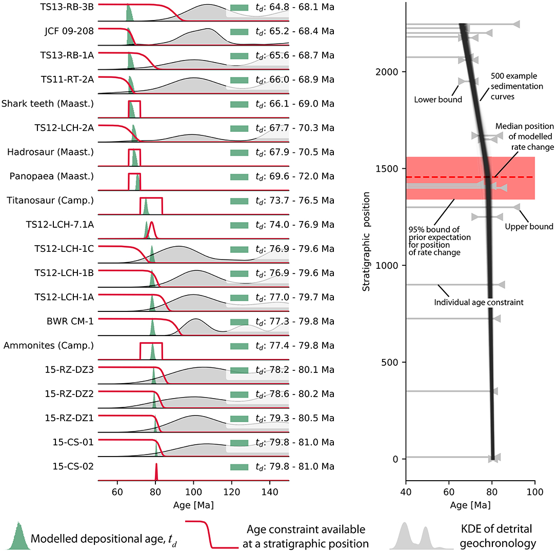
Figure 10. Results of modeling the stratigraphic accumulation rate of the Magallanes basin based on geochronologic constraints. Each row shows a KDE constructed with a gaussian kernel with a bandwidth equal to the mean 2σ uncertainty of samples if that row corresponds to a detrital geochronology sample, the likelihood of a depositional age given the data available for that deposit as a red line, and the posterior probability of the depositional age of that unit as a green histogram of MCMC samples with 50 evenly spaced bins. In each of these plots the legend indicates the 95% credible interval for the modeled true depositional age, t_d and, for detrital geochronology samples, the MDA, t_e, determined with the approach of Keller et al. (2018). Right panel depicts the allowable ranges of ages for each sample, shown by gray horizontal lines, positioned vertically at their respective stratigraphic positions and extending horizontally from the point at which the likelihood function exceeds 1% of its mass to the point where it decreases below 1% of its mass; note that the age constraints are not distributed equally throughout the section. The gray horizontal age constraints do not factor in the geologic constraint imposed by superposition. Stacked, semi-transparent black lines are a subset of the probable stratigraphic accumulation rate solutions drawn from the MCMC samples. Red dashed line and box indicate the median modeled position of a change in sediment accumulation rate and the 95% bound of our prior expectation based on facies transitions (Schwartz and Graham, 2015).

FIGURE 11

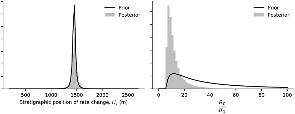
Figure 11. Prior and posterior probabilities (e.g., our initial knowledge and modeled inference) on the stratigraphic position of a change in rate (H_c) and the relative stratigraphic accumulation rates above and below that transition. Prior distributions are shown as solid black lines, posterior distributions are shown as normalized histograms of MCMC samples after the burn-in period.

Alternative depositional histories could also explain the observed geochronology. One such explanation would be the presence of an unconformity at approximately 1,670 m (the location of the observed Titanosaur), above and below which point all geochronologic constraints could be described by a near-instantaneous rate of deposition (Figure 10). In this model, one could effectively describe the observed geochronology with three variables; an age of material below an unconformity, above the unconformity, and the duration of the unconformity. Although an unconformity separating two rapidly deposited accumulations of sediment could explain the geochronologic data from the Magallanes basin (Figure 10), the detailed observational record does not currently support this. No major erosion surfaces, well-developed soils, or dramatic changes in lithofacies have been observed in this interval (Schwartz and Graham, 2015). While the models introduced here produce predictions of deposit ages that are subject to our interpretations of the geologic record, it is for that same reason that we argue they are constructive, as they provide testable prediction for our hypotheses of geologic histories. In the case presented here, the available geochronology can not refute those predictions.

Our model of stratigraphic accumulation rate is derived from the expectation that the stratigraphy represents steady, uninterrupted progradation of a shelf-slope system through the Magallanes foredeep on a multi-Myr scale. This assumption for the model is consistent with observed stratigraphic patterns that suggest (1) progressive southward progradation of the shelf and slope in Late Cretaceous time; 2) maintained genetic linkage between the Dorotea shelf and Tres Pasos slope (at least at the scale of outcrop exposure); and 3) a lack of significant unconformities within the Tres Pasos-Dorotea succession (Hubbard et al., 2010; Romans et al., 2010; Schwartz and Graham, 2015; Schwartz et al., 2017; Daniels et al., 2018a). We note that this is a highly simplified model that does not account for sub-Myr sedimentary processes (e.g., deltaic lobe-switching), variable subsidence patterns, or compaction (which could preferentially impact the finer grain sizes observed on the slope, and thus produce values of $\frac{S_0}{S_1}$ larger than $\frac{R_0}{R_1}$, similar to what we observe here). Rather, this model is an assumption of long-term (multi-Myr), "average" sedimentation patterns consistent with a highly generalized interpretation of the stratigraphy (e.g., Figures 6B, 8, after Schwartz et al., 2017).

4. Discussion and Conclusion

Sedimentary deposits are no older than their youngest mineral constituent, and efforts to calculate maximum depositional ages from detrital geochronology often rely on weighted means that are calculated based on defined groups of young grains (see Coutts et al., 2019, and references therein). Given the typical numbers of grains analyzed in detrital zircon geochronology studies (n ~100, Sharman et al., 2018; Coutts et al., 2019), we can be fairly certain that we will capture at least three grains from the youngest population if that population comprises ~10% of all zircons (Figure 2, see Andersen, 2005, for a more complete discussion). However, caution should be taken as this limits how often we should expect to see certain rare, young populations. Only in ~10% of studies of 100 grains would we expect to date three of the youngest grains if grains of that age only made up ~1% of dateable zircons.

Superposition (or any cross cutting relationship) provides an additional constraint on the ages of deposits. Utilizing Bayesian statistics to enforce this principle has long been a tactic of archeological and paleoenvironmental studies that infer depositional ages from geochronologic data (e.g., Naylor and Smith, 1988; Buck et al., 1992; Christen et al., 1995; Blaauw and Christen, 2005; Haslett and Parnell, 2008; Parnell et al., 2008; Bronk Ramsey, 2009; Blaauw, 2010; Blaauw and Christeny, 2011). Given some additional constraints that provide minimum limiting ages for deposits, these Bayesian approaches can be used to determine true depositional ages for deposits where only maximum depositional age constraints are present. While it is straightforward enough to qualitatively interpret ages with stratigraphic relationships in mind, placing these in a Bayesian framework enables inference of true depositional ages and their uncertainties (e.g., Figure 5). In spite of variations in the lag time between crystal formation and deposition, this approach makes predictions for the depositional ages of samples from the Magallanes basin with credible age intervals that span 4 Ma (Figure 7). While we achieve this degree of precision with limited direct constraints on depositional ages, this is also a favorable example. Situations with greater uncertainties on the samples that are directly dated or larger gaps between the youngest ages of zircons low in the section and constraints that provide lower limits on ages high in the sections will be met with greater uncertainty (Figure 1).

Here we determine age constraints, and assign the likelihood of depositional ages for each deposit, independently of modeling true depositional ages. The independence of these two steps results in some distributions of lag time that unrealistically span 0 Ma (Figure 7B). Future efforts can improve upon this by simultaneously solving for MDAs and t_d and, for example, enforcing the prior expectation that t_e > t_d. Such an approach might enable greater confidence in MDAs that depended on a small number of grains, as it would require these MDAs be consistent with other information in the stratigraphic section and therefore could help to reject observations from inconsistent grains that might by the product of contamination or Pb loss. The posterior probabilities of depositional ages inferred here are dependent on our characterization of the likelihood of a true depositional age given a suite of detrital geochronology ages (Equation 7 & Figure 4). Rather than the method of estimating t_e that we apply here (Keller et al., 2018), another alternative would be to determine the most likely true ages contained within a detrital geochronology sample using a mixture modeling approach that placed emphasis on identification of the youngest component (Vermeesch, 2018). The youngest true component age determined by the mixture model, and its uncertainty, could then be used to define the likelihood of a true depositional age (Equation 9).

Describing the entire stratigraphic section with a sedimentation rate curve provides a way to propagate age constraints to samples at the top of a stratigraphic section that are only characterized by MDAs (Figure 10). In our example from the Magallanes basin, the uppermost four age constraints are all obtained from detrital zircon analyses. Had we viewed these samples individually, each of them could be well-described by any age < 92 Ma, but given our model of stratigraphic accumulation rate, the uppermost unit (TS13-RB-3B) has a predicted age of 64.8–68.1 Ma. Here we prescribe the form of this sedimentation rate curve in order to replicate expectations from a simple conceptual model of a prograding shelf-slope break (Figure 8). This in turn allows us to inform our inference of ancient deposition rates with expectations derived from measurements of modern depositional systems (Figure 9). Rather than specifying a form to the deposition rate curve, there are many existing tools for more flexibly determining how sedimentation rates might vary through time, some of which can also enable introduction of expectations of hiatuses or inflections in deposition rates derived from sedimentologic observations (e.g., Blaauw and Christen, 2005; Haslett and Parnell, 2008; Parnell et al., 2008; Bronk Ramsey, 2009; Blaauw, 2010; Blaauw and Christeny, 2011).

Our model of sedimentation rates (Figure 10) produces parameter estimates that overlap significantly with the prior expectations we derive based on sedimentology (Schwartz et al., 2017) and measurements of modern depositional systems (Figures 9, 11). It is easy to imagine two seemingly conflicting interpretations of the observation that the posterior probabilities significantly overlap the prior probabilities: (1) that through asserting these prior probabilities we have forced a particular outcome, or (2) that the data we do have is consistent with our expectations for this system. A more conservative statement would be to acknowledge both points: the available geochronologic constraints do not provide information that is either contrary to our expectation or in support of a more precise quantification of the rates of stratigraphic accumulation or the point in the stratigraphic section at which they change.

The probabilities of ages we report here (Figures 7, 10) are explicitly linked to the model that generated them. As a result, model ages covary with one another. In the stratigraphic accumulation model (Figure 10), the detrital zircon sample from sedimentary unit 15-CS-01 that immediately overlies the ID-TIMS dated ash sample 15-CS-02 has a similarly precise posterior. We do not take that to mean that the timing of deposition is equally well-known for both samples; rather, this implies that both samples are similarly constrained given our model of the deposition history. In general, we have attempted to show how coupling geologic insights with geochronology can improve our understanding of sedimentary sections and can expand the inferences we can make from sections with detrital records of maximum depositional ages. The routine practice in geology of enforcing stratigraphic order in interpretation of the ages of deposits from MDAs is inherently Bayesian. Building this knowledge into a statistical model can provide a cascade of information through series of samples that can improve our characterization of geologic histories.

Author Contributions

The idea for this manuscript arose from discussions between all coauthors. SJ drafted the manuscript and preformed the modeling. TS wrote the geologic settings sections, selected the modern analog profiles, provided the data and geologic framework for the example study, and provided the idea for coupling stratigraphic interpretations with the model. CH-D edited the manuscript, provided insight on ideal example locations, helped guide the formulation of the maximum depositional age function, and guided the sections of the manuscript motivating this alternative approach to maximum depositional ages.

Funding

Support for this work came from the FEDMAP component of the US Geological Survey National Cooperative Geologic Mapping Program and from the Mineral Resources Program.

Conflict of Interest Statement

The authors declare that the research was conducted in the absence of any commercial or financial relationships that could be construed as a potential conflict of interest.

Acknowledgments

We thank L.E. Morgan for introduction to the concept of enforcing stratigraphic ordering into geochronology data. Early conversations with G. Sharman and M. Malkowski inspired this manuscript and discussion with S. Hubbard and D. Coutts provided further insights into maximum depositional ages. Editorial comments from B. Romans and two reviews substantively improved the clarity and direction of this manuscript. This draft manuscript is distributed solely for purposes of scientific peer review. Its content is deliberative and predecisional, so it must not be disclosed or released by reviewers. Any use of trade, firm, or product names is for descriptive purposes only and does not imply endorsement by the U.S. Government.

References

Amante, C., and Eakins, B. W. (2009). ETOPO1 1 Arc-Minute Global Relief Model: Procedures, Data Sources and Analysis. NOAA Technical Memorandum NESDIS NGDC-24. National Geophysical Data Center; NOAA.

Amidon, W. H., Burbank, D., and Gehrels, G. (2005). U–Pb zircon ages as a sediment mixing tracer in the Nepal Himalaya. Earth Planet. Sci. Lett. 235, 244–260. doi: 10.1016/j.epsl.2005.03.019

CrossRef Full Text | Google Scholar

Andersen, T. (2005). Detrital zircons as tracers of sedimentary provenance: Limiting conditions from statistics and numerical simulation. Chem. Geol. 216, 249–270. doi: 10.1016/j.chemgeo.2004.11.013

CrossRef Full Text | Google Scholar

Bernhardt, A., Jobe, Z. R., and Lowe, D. R. (2011). Stratigraphic evolution of a submarine channel-lobe complex system in a narrow fairway within the Magallanes foreland basin, Cerro Toro Formation, southern Chile. Mar. Petrol. Geol. 28, 785–806. doi: 10.1016/j.marpetgeo.2010.05.013

CrossRef Full Text | Google Scholar

Biddle, K. T., Uliana, M. A., Mitchum, R. M., Fitzgerald, M. G., and Wright, R. C. (1986). “The stratigraphic and structural evolution of the central and eastern magallanes basin, Southern South America,” in Foreland Basins, eds P. A. Allen and P. Homewood. doi: 10.1002/9781444303810.ch2

CrossRef Full Text | Google Scholar

Blaauw, M. (2010). Methods and code for 'classical' age-modelling of radiocarbon sequences. Quatern. Geochronol. 5, 512–518. doi: 10.1016/j.quageo.2010.01.002

CrossRef Full Text | Google Scholar

Blaauw, M., and Christen, J. A. (2005). Radiocarbon peat chronologies and environmental change. J. R. Stat. Soc. Ser. C Appl. Stat. 54, 805–816. doi: 10.1111/j.1467-9876.2005.00516.x

CrossRef Full Text | Google Scholar

Blaauw, M., and Christen, J. A. (2011). Flexible paleoclimate age-depth models using an autoregressive gamma process. Bayesian Anal. 6, 457–474. doi: 10.1214/11-BA618

CrossRef Full Text | Google Scholar

Brandon, M. T., and Vance, J. A. (1992). Tectonic evolution of the Cenozoic Olympic subduction complex, Washington State, as deduced from fission track ages for detrital zircons. Am. J. Sci. 292, 565–636. doi: 10.2475/ajs.292.8.565

CrossRef Full Text | Google Scholar

Bronk Ramsey, C. (2009). Bayesian analysis of radiocarbon dates. Radiocarbon 51, 337–360. doi: 10.1017/S0033822200033865

CrossRef Full Text | Google Scholar

Buck, C. E., Litton, C. D., and Smith, A. F. (1992). Calibration of radiocarbon results pertaining to related archaeological events. J. Archaeol. Sci. 19, 497–512. doi: 10.1016/0305-4403(92)90025-X

CrossRef Full Text | Google Scholar

Carvajal, C., and Steel, R. (2009). Shelf-edge architecture and bypass of sand to deep water: influence of shelf-edge processes, sea level, and sediment supply. J. Sediment. Res. 79, 652–672. doi: 10.2110/jsr.2009.074

CrossRef Full Text | Google Scholar

Christen, J. A., Clymo, R. S., and Litton, C. D. (1995). A Bayesian approach to the use of 14C dates in the estimation of the age of peat. Radiocarbon 37, 431–441. doi: 10.1017/S0033822200030915

CrossRef Full Text | Google Scholar

Coutts, D. S., Matthews, W. A., and Hubbard, S. M. (2019). Assessment of widely used methods to derive depositional ages from detrital zircon populations. Geosci. Front. doi: 10.1016/j.gsf.2018.11.002

CrossRef Full Text | Google Scholar

Covault, J. A., Romans, B. W., and Graham, S. A. (2009). Outcrop expression of a continental-margin-scale shelf-edge delta from the Cretaceous Magallanes Basin, Chile. J. Sediment. Res. 79, 523–539. doi: 10.2110/jsr.2009.053

CrossRef Full Text | Google Scholar

Dalziel, I. W., De Wit, M. J., and Palmer, K. F. (1974). Fossil marginal basin in the southern Andes. Nature 250, 291–294. doi: 10.1038/250291a0

CrossRef Full Text | Google Scholar

Dalziel, I. W. D. (1981). Back-Arc extension in the Southern Andes: a review and critical reappraisal. Philos. Trans. R Soc A Math Phys Eng Sci. 300, 319–335.

Google Scholar

Daniels, B. G., Auchter, N. C., Hubbard, S. M., Romans, B. W., Matthews, W. A., and Stright, L. (2018a). Timing of deep-water slope evolution constrained by large-n detrital and volcanic ash zircon geochronology, Cretaceous Magallanes Basin, Chile. Bull. Geol. Soc. Am. 130, 438–454. doi: 10.1130/B31757.1

CrossRef Full Text | Google Scholar

Daniels, B. G., Kaempfe, S., Hubbard, S. M., Romans, B. W., and Matthews, W. A. (2018b). “The influence of Andean orogenic uplift and deformation style on the evolution of stratigraphic architecture, Cretaceous Magallanes foreland basin, Chilean Patagonia,” in XV Congreso Geológico Chileno Actas, 1156.

Google Scholar

Dickinson, W. R., and Gehrels, G. E. (2009). Use of U-Pb ages of detrital zircons to infer maximum depositional ages of strata: a test against a Colorado Plateau Mesozoic database. Earth Planet. Sci. Lett. 288, 115–125. doi: 10.1016/j.epsl.2009.09.013

CrossRef Full Text | Google Scholar

Fildani, A., and Hessler, A. M. (2005). Stratigraphic record across a retroarc basin inversion: Rocas Verdes-Magallanes Basin, Patagonian Andes, Chile. Bull. Geol. Soc. Am.117, 1596–1614. doi: 10.1130/B25708.1

CrossRef Full Text | Google Scholar

Foreman-Mackey, D., Hogg, D. W., Lang, D., and Goodman, J. (2013). emcee : the MCMC Hammer. Publ. Astron. Soc. Pacific 125, 306–312. doi: 10.1086/670067

CrossRef Full Text | Google Scholar

Fosdick, J. C., Graham, S. A., and Hilley, G. E. (2014). Influence of attenuated lithosphere and sediment loading on flexure of the deep-water Magallanes retroarc foreland basin, Southern Andes. Tectonics 33, 2505–2525. doi: 10.1002/2014TC003684

CrossRef Full Text | Google Scholar

Fosdick, J. C., Grove, M., Graham, S. A., Hourigan, J. K., Lovera, O., and Romans, B. W. (2015). Detrital thermochronologic record of burial heating and sediment recycling in the Magallanes foreland basin, Patagonian Andes. Basin Res. 27, 546–572. doi: 10.1111/bre.12088

CrossRef Full Text | Google Scholar

Fosdick, J. C., Romans, B. W., Fildani, A., Bernhardt, A., Calderon, M., and Graham, S. A. (2011). Kinematic evolution of the Patagonian retroarc fold-and-thrust belt and Magallanes foreland basin, Chile and Argentina, 51 30'S. Geol. Soc. Am. Bull. 123, 1679–1698. doi: 10.1130/B30242.1

CrossRef Full Text | Google Scholar

Gorelick, N., Hancher, M., Dixon, M., Ilyushchenko, S., Thau, D., and Moore, R. (2016). Google Earth Engine: Planetary-scale geospatial analysis for everyone. Remote Sens. Environ. 202, 18–27. doi: 10.1016/j.rse.2017.06.031

CrossRef Full Text | Google Scholar

Haslett, J., and Parnell, A. (2008). A simple monotone process with application to radiocarbon-dated depth chronologies. J. R. Stat. Soc. Ser. C Appl. Stat. 57, 399–418. doi: 10.1111/j.1467-9876.2008.00623.x

CrossRef Full Text | Google Scholar

Hubbard, S. M., Fildani, A., Romans, B. W., Covault, J. A., and McHargue, T. R. (2010). High-relief slope clinoform development: insights from outcrop, Magallanes Basin, Chile. J. Sediment. Res. 80, 357–375. doi: 10.2110/jsr.2010.042

CrossRef Full Text | Google Scholar

Keller, C. B., Schoene, B., and Samperton, K. M. (2018). A stochastic sampling approach to zircon eruption age interpretation. Geochem. Persp. Lett. 8, 31–35. doi: 10.7185/geochemlet.1826

CrossRef Full Text | Google Scholar

Kruschke, J. K. (2013). Bayesian estimation supersedes the t test. J. Exp. Psychol. Gen. 142, 573–603. doi: 10.1037/a0029146

PubMed Abstract | CrossRef Full Text | Google Scholar

Macellari, C. E., Barrio, C. A., and Manassero, M. J. (1989). Upper cretaceous to paleocene depositional sequences and sandstone petrography of southwestern Patagonia (Argentina and Chile). J. South Am. Earth Sci. 2, 223–239. doi: 10.1016/0895-9811(89)90031-X

CrossRef Full Text | Google Scholar

Malkowski, M. A., Sharman, G. R., Graham, S. A., and Fildani, A. (2017). Characterisation and diachronous initiation of coarse clastic deposition in the Magallanes-Austral foreland basin, Patagonian Andes. Basin Res. 29, 298–326. doi: 10.1111/bre.12150

CrossRef Full Text | Google Scholar

Natland, M. L., Eduardo, G. P., Cañon, A., and Ernst, M. (1974). “A system of stages for correlation of magallanes basin sediments,” in Geological Society of America (Boulder, CO), 1–126. doi: 10.1130/MEM139

CrossRef Full Text | Google Scholar

Naylor, J. C., and Smith, A. F. M. (1988). An archaeological inference problem. J. Am. Stat. Assoc. 83, 588–595. doi: 10.1080/01621459.1988.10478638

CrossRef Full Text | Google Scholar

Parnell, A. C., Buck, C. E., and Doan, T. K. (2011). A review of statistical chronology models for high-resolution, proxy-based Holocene palaeoenvironmental reconstruction. Quatern. Sci. Rev. 30, 2948–2960. doi: 10.1016/j.quascirev.2011.07.024

CrossRef Full Text | Google Scholar

Parnell, A. C., Haslett, J., Allen, J. R., Buck, C. E., and Huntley, B. (2008). A flexible approach to assessing synchroneity of past events using Bayesian reconstructions of sedimentation history. Quatern. Sci. Rev. 27, 1872–1885. doi: 10.1016/j.quascirev.2008.07.009

CrossRef Full Text | Google Scholar

Romans, B. W., Castelltort, S., Covault, J. A., Fildani, A., and Walsh, J. P. (2016). Environmental signal propagation in sedimentary systems across timescales. Earth Sci. Rev. 153, 7–29. doi: 10.1016/j.earscirev.2015.07.012

CrossRef Full Text | Google Scholar

Romans, B. W., Fildani, A., Graham, S. A., Hubbard, S. M., and Covault, J. A. (2010). Importance of predecessor basin history on sedimentary fill of a retroarc foreland basin: provenance analysis of the Cretaceous Magallanes basin, Chile (50-52°S). Basin Res. 22, 640–658. doi: 10.1111/j.1365-2117.2009.00443.x

CrossRef Full Text | Google Scholar

Schwartz, T. M., Fosdick, J. C., and Graham, S. A. (2017). Using detrital zircon U-Pb ages to calculate Late Cretaceous sedimentation rates in the Magallanes-Austral basin, Patagonia. Basin Res. 29, 725–746. doi: 10.1111/bre.12198

CrossRef Full Text | Google Scholar

Schwartz, T. M., and Graham, S. A. (2015). Stratigraphic architecture of a tide-influenced shelf-edge delta, Upper Cretaceous Dorotea Formation, Magallanes-Austral Basin, Patagonia. Sedimentology 62, 1039–1077. doi: 10.1111/sed.12176

CrossRef Full Text | Google Scholar

Sharman, G. R., Sharman, J. P., and Sylvester, Z. (2018). detritalPy: A Python-based toolset for visualizing and analysing detrital geo-thermochronologic data. Depos. Rec. 4, 202–215. doi: 10.1002/dep2.45

CrossRef Full Text | Google Scholar

VanderPlas, J. (2014). Frequentism and Bayesianism: a Python-driven Primer. arXiv, astro-ph.I(Scipy):1–9.

Google Scholar

Vermeesch, P. (2012). On the visualisation of detrital age distributions. Chem. Geol. 312–313, 190–194. doi: 10.1016/j.chemgeo.2012.04.021

CrossRef Full Text | Google Scholar

Vermeesch, P. (2018). IsoplotR: A free and open toolbox for geochronology. Geosci. Front. 9, 1479–1493. doi: 10.1016/j.gsf.2018.04.001

CrossRef Full Text | Google Scholar

Walker, J. D., Geissman, J. W., Bowring, S. A., and Babcock, L. E. (2018). Geologic Time Scale v. 5.0. Geol. Soc. Am. 125, 259–272. doi: 10.1130/B30712.1

CrossRef Full Text | Google Scholar

Wilson, T. J. (1991). Transition from back-arc to foreland basin development in the southernmost Andes: stratigraphic record from the Ultima Esperanza District, Chile. Geol. Soc. Am. Bull. 103, 98–111.

Google Scholar