Robust Characteristics of the Laschamp and Mono Lake Geomagnetic Excursions: Results From Global Field Models

1. Introduction

The geomagnetic main field varies on a broad temporal range. From years to decades, spherical harmonic (SH) core field models based on data from ground-based observatories and satellites provide an increasingly detailed view of the spatial and temporal evolution of the global geomagnetic field (e.g., Lesur et al., 2011; Hulot et al., 2015). Such models allow the geomagnetic field to be mapped at the core-mantle boundary (CMB), allowing investigation into core dynamics and the geodynamo process.

Models of the historical field (Jackson et al., 2000) and a growing number of models based on archeo- and paleomagnetic data covering the past 2 to 14 millennia (e.g., Korte et al., 2011; Licht et al., 2013; Nilsson et al., 2014; Pavón-Carrasco et al., 2014; Panovska et al., 2015; Constable et al., 2016) have improved our understanding of global field evolution on centennial to millennial time-scales (e.g., Constable and Korte, 2015). However, we lack a good understanding of the global geomagnetic field during more extreme changes in the field, such as reversals and excursions. These events have occurred numerous times in the geological past (Singer, 2014; Laj and Channell, 2015) and are relevant for understanding the full range of geodynamo behavior. Individual records, however, provide a limited view for understanding the global excursion dynamics.

To date there have been only a small number of attempts to develop global SH models of reversals and excursions. Initial models used time snapshots of the field (Mazaud, 1995; Shao et al., 1999; Ingham and Turner, 2008). More recent models implemented temporal continuity and expanded SH basis functions to degree and order 5 (Leonhardt and Fabian, 2007; Lanci et al., 2008; Leonhardt et al., 2009), but all these models are based on limited global data coverage. Brown et al. (2018) presented the first model (LSMOD.1) spanning both the Laschamp and Mono Lake (~33 ka) excursions with the time interval 50 to 30 ka and based on 12 sediment records. The first continuous SH model continuously spanning the past 100 kyr (GGF100k) was recently derived by Panovska et al. (2018b), constrained by more than 100 sediment records. These two models include all volcanic data that were available at the time.

Reversals are full global polarity changes of the geomagnetic field. However, the global nature of excursions is less well-known. Many paleomagnetic records indicate that intensity generally weakens during excursions (as during reversals), but accompanying transitional directions have not always been observed globally (e.g., Roberts, 2008; Laj and Channell, 2015). This may reflect field behavior or may result from imperfections in the sedimentary recording mechanism. Post-depositional remanent magnetization acquisition processes may act as a low-pass filter, so that the excursional signal might be completely smoothed out by the combination of a low sedimentation rate and lock-in depth (Roberts and Winklhofer, 2004). Moreover, both sedimentation rate and lock-in depth may vary within a sediment record, increasing age uncertainties further (e.g. Sagnotti et al., 2005). The intensity low in general seems to last longer than the strong directional changes, and in particular fast directional excursion signals might not be recorded.

However, we should not necessarily expect to find transitional or reversed directions everywhere on Earth during an excursion (e.g., Leonhardt et al., 2009). Brown and Korte (2016) demonstrated, by using a toy model, that this would be the case if the excursion process was governed purely by decay and recovery of axial dipole strength, and smaller scale secular variation continued as during the past millennia. In that scenario, the directional excursion signal varies strongly by region. Even with the axial dipole decreased to zero there are areas that show little directional variation. Globally reversed directions only appeared in the model when the axial dipole was reversed and gained at least 20% of pre-excursional strength in the opposite direction at the excursion midpoint. It seems conceivable that the geomagnetic field can show a broad range of excursional behavior depending on the reduction in strength of the axial dipole and whether it reverses, and on the role of equatorial dipole and non-dipole fields. This suggests that the global surface field morphology during an excursion can be non-uniform and that different excursions can display different surface field behavior, a result that was also found in a recent statistical analysis of high resolution paleomagnetic sediment records from three different regions on Earth (Lund, 2018).

Here, we analyse a suite of new SH models spanning 50 to 30 ka, which include the Laschamp (~41 ka) and Mono Lake (~33 ka) excursions. For comprehensive reviews of paleomagnetic and geochronological studies on these excursions, see Laj and Channell (2015) and Singer (2014). Our models are built from sediment and volcanic paleomagnetic data. The main aim of our study is to investigate the global geomagnetic field behavior during these excursions. Uncertainties regarding magnetic field recording fidelity and accuracy of dating of the paleomagnetic data suggest that model errors might be larger than one would estimate from considering only one data set. Therefore we investigate a range of models, giving different weight to individual records by using them individually or stacking them regionally, and making different assumptions about the contemporaneity of the intensity minimum seen at different locations. We assess the influence of these data variations on the geomagnetic field structures produced by our models, compare them to existing models, and determine which characteristics are robust to all models. Although volcanic data are included in our models, these data and their uncertainties have a minor influence on the models due to their sparsity.

In section 2 the data sets for our new models are summarized, and we outline how they differ to those used for the previously published models IMOLEe (44–36 ka) (Leonhardt et al., 2009) and GGF100k (100–0 ka) (Panovska et al., 2018b). The modeling method is described in section 3, including tests on reconstructing known fields from synthetic data. Several global characteristics of the models and their robustness depending on variations of the underlying data are described in section 4. They are also compared with findings from IMOLEe and GFF100k. A slightly updated version of LSMOD.1 is included in our suite of models. This is our preferred model and is made available under the name LSMOD.2 (http://doi.org/10.5880/GFZ.2.3.2019.001). Potential implications of our findings regarding the excursion process are discussed in section 5 before concluding with an outlook.

2. Data and Existing Models

All of our data sets combine volcanic data and high resolution sediment records spanning 50 to 30 ka.

2.1. Volcanic Data

The volcanic data compilation is the same as used by Brown et al. (2018). It consists of 65 inclinations, 64 declinations and 41 paleointensities (Figure 1) (including results from a fired archeological site in Australia). Details are given in the supplement of Brown et al. (2018). With the exception of data from New Zealand and Australia, all volcanic data are from the Northern hemisphere. The volcanic data set was not varied for the different models.

FIGURE 1

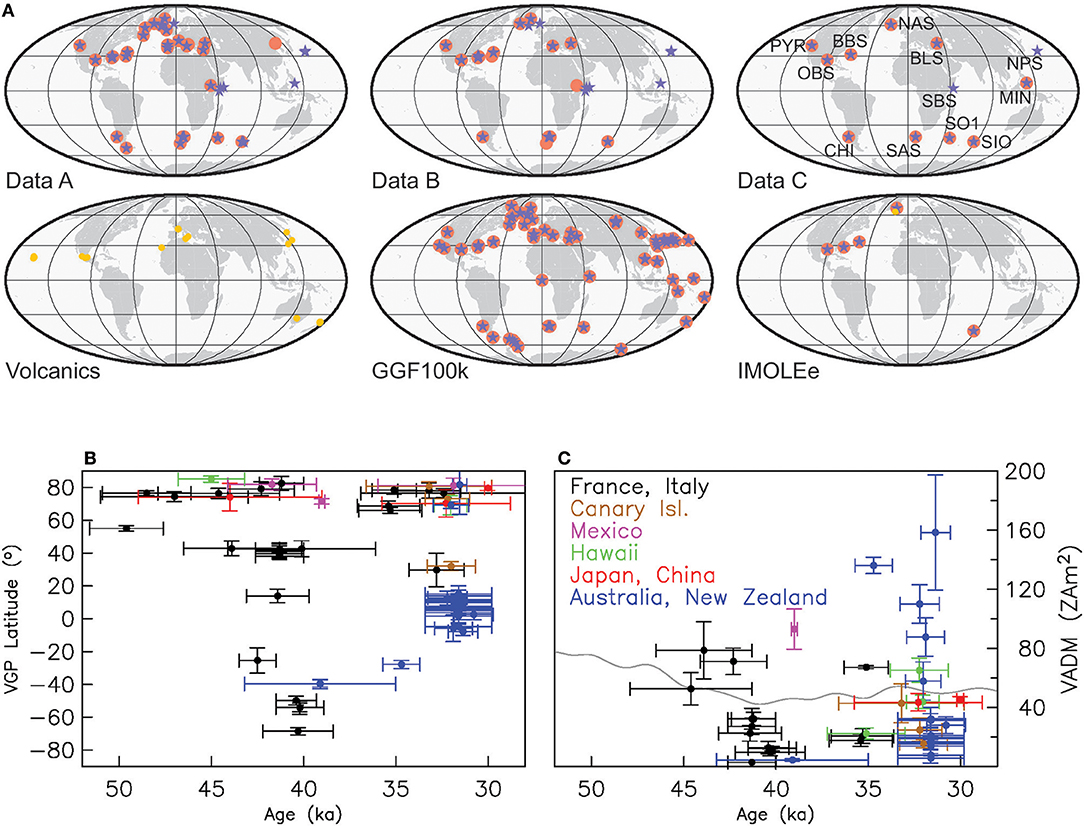
Figure 1. Spatial data distribution for the models investigated in this study (A). Red dots indicate locations with directional and blue stars with intensity data, for the different models. Orange dots (bottom left) indicate the locations of volcanic data. Their distribution for GGF100k is very similar, whereas IMOLEe (bottom right) includes only one volcanic record from Iceland indicated in that panel by an orange dot. Volcanic data are unevenly distributed in time, both for directions (B) and intensity (C). Volcanic results from one region hardly cover the full time interval. The gray line intensity time series in (C) is the axial dipole moment reconstruction PADM2M (Ziegler et al., 2011) used for our sediment RPI scaling.

2.2. Sediment Records

Our data set is dominated by sediment records. They provide more uniform time series for individual sites and regions than volcanic data. We use the global set of directional and relative paleointensity (RPI) records, fully or partly spanning the 50–30 ka time interval, as compiled by Brown et al. (2018) and summarized in Table S1. The variations of the complete data set used for our suite of models are described in section 2.2.2

2.2.1. RPI Calibration, Declination Orientation, and Age Control

Sediment paleomagnetic records cannot provide information on absolute paleointensity, they only give variations in RPI if the measurements can be suitably normalized (see, e.g., Tauxe and Yamazaki, 2015). It is therefore necessary to calibrate these data to absolute values. Ideally this would be done by using nearby absolute intensity results from volcanics, but this is not possible owing to the sparse spatio-temporal distribution of volcanic data in the time interval of interest (Figure 1). We therefore calibrated each RPI record by comparison to the global axial dipole moment reconstruction PADM2M by Ziegler et al. (2011), as described in detail by Brown et al. (2018).

Sediment cores are in general not oriented azimuthally, and declinations are determined as relative values. Ideally the rotation to absolute values could be done using nearby oriented volcanic data. However, as with intensity data, the spatial and temporal sparsity of volcanic declinations often means this approach is not feasible. Most commonly, sediment declination records are rotated so that their mean declination is zero. It is important to consider both the method of core rotation and the period of time over which the rotation is performed (see, e.g., Korte et al., 2019), as this influences virtual geomagnetic pole (VGP) positions and, therefore, the investigation of preferred VGP paths. In general we used declination data oriented to zero mean over the full length of the published record. Note that this is one source of difference between our new models and IMOLEe (Leonhardt et al., 2009). Leonhardt et al. (2009) used the Southern Indian Ocean record MD94-103 (location called SIO here, see Figure 1) spanning 44–37 ka as presented in Laj et al. (2006). However, we used a longer version of this record (Mazaud et al., 2002), which has a different zero mean declination.

Dating is another critical point. In order to avoid any prior assumption about the timing of the excursions at different locations we used each record with the most current independent age information. Ages of lavas constrained by radiocarbon dates were re-calibrated using the most recent ¹⁴C calibration curves, i.e., IntCal13 (Reimer et al., 2013) and SHCal13 (Hogg et al., 2013) for the northern and southern hemisphere, respectively (see Brown et al., 2018).

Sediment records with chronologies based purely on directional or RPI correlation to another record or global/regional stack do not provide independent paleomagnetic information and were not used. Some studies combine independent age control and paleomagnetic dating and we included five such records. Depth-age models of several sediment records were updated, especially when new age information had become available since the original publication date. Radiocarbon ages were recalibrated using the most recent calibration curves (Hogg et al., 2013; Reimer et al., 2013). Chronologies based upon older δ¹⁸O reference records were adjusted to more recently published ones. The Greenland Ice Sheet Project 2 (GISP2) chronology (Meese et al., 1997) was transferred to the Greenland Ice Core Chronology (GICC05) time scale (Svensson et al., 2008) using the algorithm of Obrochta et al. (2014). Age tie points based on the SPECMAP δ¹⁸O chronology were converted to the U/Th derived chronology of Thompson and Goldstein (2006). Details of all chronologies and their adjustments are given in the supplement to Brown et al. (2018).

2.2.2. Variations on Data for a Suite of Models

Several factors limit the reliability and temporal resolution of paleomagnetic measurements. All sediment records are smoothed representations of the magnetic field signal, depending on a combination of the remanence acquisition process, sedimentation rate, potential influence of diagenesis, and sampling method (see, e.g., Roberts and Winklhofer, 2004; Roberts et al., 2013; Roberts, 2015; Philippe et al., 2018; Sagnotti, 2018). This may result in the directional changes of short excursions not or only partially being recorded, or distorted. The accuracy and precision of chronological data and associated age models dictate whether a reliable time series of paleomagnetic field variations can be obtained. Poorly constrained age models may result in age offsets between records that are not geomagnetic in origin.

Another difficult issue is whether the measured sediment magnetization can be normalized to reliably reflect RPI (see, e.g., Tauxe and Yamazaki, 2015). Environmental influences and insufficient understanding of the remanance acquisition process may strongly limit the reliability of the recovered magnetic intensity signal. This can result in inconsistent RPI variations in records from neighboring locations. Even with detailed rock magnetic and sedimentological analyses it is not always clear which records reliably capture RPI variations.

To understand which model characteristics are robust and independent of subjective assumptions about the data, we built more than 20 models based on different (sub)sets of data with variations in assumptions on data reliability and their age-models. Variations in assumed reliability are expressed in the modeling process by varying the relative weighting by stacking or rejection of some records. Potential influences of dating uncertainties were considered by regional or global age alignment of the records.

To simplify the analysis we show results from four models representative of our suite of models. They are based upon data sets A to D, which are summarized in Table 1 and their locations are shown in Figure 1. The coordinates of the records and further details are given in Supplement S1.

TABLE 1

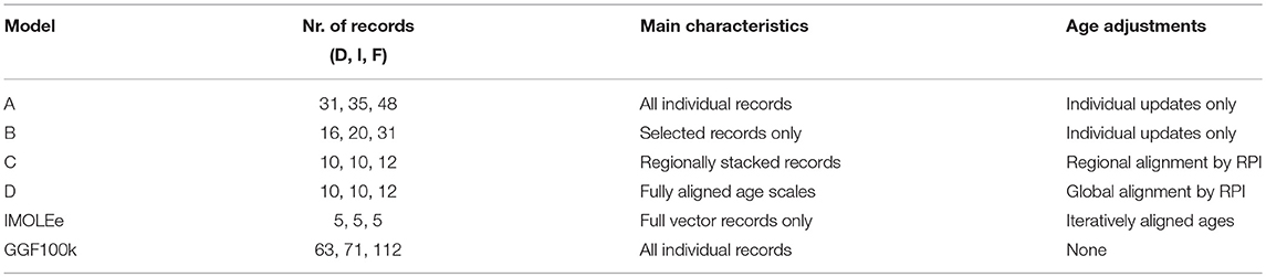
Table 1. Characteristics of sediment data sets underlying the models.

Data set A consists of all individual available sediment records and can be considered as an end member utilizing the available information with least additional assumptions, and no further corrections than described in section 2.2.1.

As seen in Figure 1, more than two records exist in relatively close proximity for some regions. Plotting these time series together revealed cases where at least two records show consistent signals in the magnetic field components (though sometimes offset in age), whereas others appear incompatible given their spatial proximity relative to the distance from the field source in Earth's core. Data set A is, therefore, not necessarily the best input for the inverse modeling, because inconsistencies in the data may smooth or distort magnetic field features in the resulting model.

To mitigate this effect, we created data sets where we removed records that appeared regionally inconsistent. To give one example for what is meant by inconsistency: consider that one record shows a clear intensity minimum around 41 ka and another, closely adjacent one does not. In that case we would have kept the record with the minimum, and discarded the other one, arguing that it seems more likely that a real field variation was smoothed out, than an excursion signal was created by environmental or sedimentary processes. Further examples are given in section 4.1, where we look at the fit of the models to the data. Data set B represents one example of such an (arguably subjective) selection.

For data set C we took into account that some signals of adjacent records look similar but offset in time. Data set C is essentially the same as used by Brown et al. (2018) for LSMOD.1, with a correction to a coordinate error in one directional data file, see Supplement S1. We adjusted the chronologies of adjacent RPI records to a master record considered to have the most reliable independent chronology, and stacked the records (see Brown et al., 2018, Supplement, for details). With very few exceptions the distances to the master record were <700 km, with a maximum distance of 1700 km for one of the records included in the North Atlantic (NAS) stack. Note that the consistency of the declination signals did not necessarily improve by this RPI-based alignment. In our opinion this data set gives the most coherent currently available information about the past global geomagnetic field evolution, and we consider the model based on data set C (model C) our preferred model. We make it available as an update to LSMOD.1 under the name LSMOD.2.

Data set D contains the same records as data set C, but we additionally aligned all records linearly so that the Laschamp intensity minimum appears uniform in all records globally, not only regionally. Although there is no reason to assume that the intensity minimum of an excursion should be seen coevally everywhere on Earth, we cannot fully rule out that possibility given the considerable uncertainties in sediment chronologies. This data set and resulting model are our other end member using strong assumptions about the timing of the Laschamp excursion at Earth's surface.

2.3. Models Used in Comparison

Two existing models are included in the comparison with our new models: IMOLEe (Leonhardt et al., 2009) and GGF100k (Panovska et al., 2018b). Information on their data sets is included in Table 1.

IMOLEe is the shortest model, spanning 44–36 ka. It includes the Laschamp, but not the Mono Lake excursion. It is based on one volcanic record from Iceland, and five full vector sediment records that were considered the most reliable at that time (see Figure 1 and Table S1). Four of them are from the North Atlantic and the Gulf of Mexico (Figure 1A). Uncertainties in the chronologies were treated in a special way: starting with a model from one record the other records were added iteratively with adjustments to the age scales for agreement with the previous iteration model.

GGF100k was optimized to span the full time interval from 100 ka to present. The modeling method is similar to our new models. The number of included records for 50–30 ka (Table 1) is higher than for our new models, because records with lower sedimentation rates were included. The temporal resolution of GGF100k is notably lower. All underlying sediment records were used as originally published, without any of the updates made to our data set.

3. Methods

3.1. Paleomagnetic Global Field Modeling

The modeling method is essentially the same as used for the CALSxk series of Holocene paleomagnetic field reconstructions (see, e.g., Korte et al., 2009, for more details than summarized in the following). In regions free from magnetic field sources the vector field B can be expressed as the negative gradient of a scalar potential, V, which is expanded in spherical harmonic (SH) functions in space:

$\begin{array}{l}V(r,\theta ,\varphi ,t)=a{\displaystyle \sum _{l=1}^{L_{max}}}{\displaystyle \sum _{m=0}^l}{\left(\frac{a}{r}\right)}^{l+1}\left[g_l^{m}cos(m\varphi )+h_l^{m}sin(m\varphi )\right]\end{array}$

$\begin{array}{ll}{P}_l^m(cos\theta ),& (1)\end{array}$

where (r, θ, ϕ) are spherical polar coordinates, a = 6371.2 km is Earth's mean radius and the $P_l^m(\text{cos}\theta )$ are Schmidt quasi-normalized associated Legendre functions of degree l and order m. A model is given by a set of time, t, dependent Gauss-coefficients $g_l^m(t),h_l^m(t)$ of SH degree l and order m up to maximum degree l = L_max, which are determined from the data by inversion. The temporal basis functions are cubic B-splines. L_max and the number of splines are chosen to allow for smaller scale structure and faster variations than expected to be resolved by the data. We chose L_max=10 and the number of splines such that models have spline knot-points every 50 years, and our models span the interval 50 to 30 ka. A close fit to the data is traded off in the inversion against regularization constraints that limit the spatial and temporal complexity by minimizing a measure, (Ψ), considered to damp short wavelength more strongly than long ones in proportion to Ohmic dissipation (Gubbins, 1975; Bloxham and Jackson, 1992; Korte et al., 2009),

$\begin{array}{ll}\Psi ={\displaystyle \sum _{l=1}^{L_{max}}}\frac{(l+1)(2l+1)(2l+3)}{l}{\left(\frac{a}{c}\right)}^{2l+3}{\displaystyle \sum _{m=0}^l}\left[{(g_l^m)}^2+{(h_l^m)}^2\right],& (2)\end{array}$

and the second time derivative of the radial field component (B_r),

$\begin{array}{ll}\Phi =\frac{1}{t_e-t_s}{\displaystyle \underset{t_s}{\overset{t_e}{\int }}}{{\displaystyle \oint }}_{CMB}{({\partial }_t^2{B}_r)}^2\text{d}\Omega \text{d}t& (3)\end{array}$

over the time interval (t_e − t_s) and the surface Ω of the core-mantle boundary. This is done in order to account for data uncertainties and to avoid unrealistic small-scale structures in the model from fitting the data too closely. The spatial and temporal complexity of the model are determined by regularization parameters λ and τ, respectively. If the uncertainties of the data were well-determined we could choose the regularization parameters to fit the data just within their uncertainties, thus obtaining the smoothest, simplest model that explains the data given their uncertainties. However, as the errors are not well-known we have to make more subjective choices. For λ, we considered that the core field power spectrum is expected to be approximately white at the core-mantle-boundary (CMB) for SH degrees ≥2, as seen in the present-day field. The regularization constraint is designed such that increasing values of λ lead to increased damping of short wavelength power, becoming a plain dipole for very large λ. If the regularization factor is weak, the spectrum rises toward small scales. The regularization strength that we consider suitable gives an approximately white spectrum for SH degrees 2 to 5 and drops quickly with higher degree, so that the effective spatial resolution of the models is no higher than SH degree ~5. To give the highest temporal resolution considered reasonable given the time series resolution, the temporal regularization parameter τ was chosen by visual comparison of the sediment input data with the model predictions.

The available magnetic field components declination, inclination and intensity are non-linearly related to the scalar potential that is expanded in the SH functions. The inversion therefore has to be linearized and solved iteratively. The largest changes to model and fit to the data are observed in the first few steps and the iteration was terminated with step 35 when convergence was reached. Outlying data rejection was not applied because the directional excursion signal might in places be too rapid to be fit properly by a regularized model. We did not want to smooth the model even more by rejecting probably realistic data. All data were weighted by uncertainty estimates in the inversion. For volcanic data these are given by the scaled α₉₅ values (see, e.g., Equations 1 and 2 in Donadini et al., 2009) and the reported intensity uncertainties, with minimum values set to α₉₅=4.3° and 5μT, respectively, as used in Holocene models. However, data uncertainties are in general not reported for sediment paleomagnetic data. Again following the practice used in Holocene models (Donadini et al., 2009) they were set to α₉₅=6° in all cases, and calibrated RPI intensities also were assigned an uncertainty of 5μT.

3.2. Tests of the Method

We performed a number of tests to ensure the robustness and reliability of model results during extreme field changes like excursions, with respect to modeling method, data distribution and influence of regularization. Data distribution plays a critical role, more important than modeling method, and we show this through a comparisons between IMOLEe and a test model based on the same five records in the Supplement S2.

3.2.1. Reconstruction of a Known Model

Although we have increased the global data basis notably compared to IMOLEe, large areas of the world remain poorly sampled by the available data (see Figure 1). The effect on resolvable structure and the influence of the required regularization can be tested by reconstructing a known model from a set of synthetic data obtained by model predictions with the spatial and temporal distribution of the actual paleomagnetic data. Brown et al. (2018) showed from tests using the historical gufm1 model (Jackson et al., 2000) that if the data were accurate we would be able to resolve structure up to SH degree and order 6 with the available data distribution. The likely not normally distributed and partly correlated errors on the paleomagnetic data lower the achievable resolution.

Another question is whether the design of our regularization constraints is suitable for a non-dipole dominated field, as might be the case during an excursion. To test this we used one of the toy models by Brown and Korte (2016), where a simple excursion mechanism was simulated over 10 kyrs by modifying the CALS10k.2 Holocene magnetic field model (Constable et al., 2016). The secular variation (SV) of the axial dipole contribution was scaled linearly to decrease from its original value at 8000 BC to 0 in 3005 BC and to increase back to its original value in 1990, while equatorial dipole coefficients and SH degrees 2 to 10 of the model were not altered. We predicted time series of the field components from this toy model at the locations of our data set A, and then reconstructed the toy model from these synthetic records.

This error-free input data set can be reproduced very closely with our modeling method. However, if the regularization is too weak, artificial small-scale structure appears, in particular during the time of weak dipole moment in the middle of the excursion. At this time there is an increase in high SH degree power in the main field and SV power spectra. This can be seen in Figure S5, where the power spectra of two reconstructions averaged over the 10 kyr, and for the simulated excursion midpoint at 3005 BC, are compared with the input model for the same times. Low degree power is similar for both reconstructions, with reasonable agreement during times of weak axial dipole in the middle of the excursion. The high degree power increases during the excursion, but this effect is small if the regularization is strong enough. We consider a flat or concave shape of the average main field and/or SV spectrum at high degrees (as seen for the higher resolution model in Figures S5A,B) as an indication for insufficient damping in our modeling strategy when using real data. The results of this exercise do not change notably if we add randomly distributed errors to the synthetic records (on the order of those estimated for the real data) or change the weighting of the data. Therefore, we consider our regularization constraints, based on the spectral power distribution, to be suitable to avoid this effect.

3.2.2. Reconstruction of a High Resolution Model

The past field at times might be less dipole dominated than the present day and historical field. Therefore, we investigated how our modeling and regularization methods perform for reconstructing models of high spatial complexity and generally weaker dipole dominance. Numerical dynamo simulations often have these characteristics. We predicted dense time-series for the locations of our available real data distribution from such a simulation (see Supplement S3 for details) for a time interval considered to be equivalent to 40 kyr based on magnetic diffusion time, and which includes an excursion. We modeled these time series up to SH degree 10, a spline knot point spacing of 50 years and chose the regularization strength according to our usual criteria of power spectral characteristics and visual comparison of model predictions and data. Comparing the original dynamo simulation with the reconstructed model (Figure S6) confirms that the available data distribution can recover structures up to SH degree 6. The model fits the data closely and, naturally, the loss of resolution for high degrees is less pronounced at the Earth's surface than the CMB. A comparison with the spectrum from the International Geomagnetic Reference Field (IGRF) for 2015 (Thébault et al., 2015) illustrates that the numerical simulation is less dipole dominated and has less power in SH degrees 2 to 5 than the present-day field.

4. Results: Robustness of Model Features and Comparison to Findings From Other Models

The four new models presented here represent the range of differences found in investigating more than 20 models based on a wider variety of (sub)sets of the available data. They are named models A to D, according to the underlying data sets (Table 1). Their regularization parameters and resulting spatial and temporal complexity, as well as normalized root mean square misfit to the data are listed in Table S4. In this section we first consider the fit to the data, then describe global features, such as dipole moment and spectral power distribution. We investigate the duration of the Laschamp and Mono Lake excursions at the CMB and Earth's surface, assess their global field morphology, and highlight differences between the two excursions. In order to get an overview over links between different model characteristics and their evolution with time we created animations depicting many of the discussed magnetic field maps and properties. They are available at the EarthRef Digital Archive https://earthref.org/ERDA/2385/ and https://earthref.org/ERDA/2386/.

4.1. Fit to the Data

The data uncertainties used for weighting in the modeling and in normalizing the root mean square (rms) misfit might not be fully realistic and we have not considered any age uncertainties. Therefore, we do not expect to fit the data to a normalized rms misfit of 1.0 (Table S4). Our regularization strategy leads to varying model complexity depending on data distribution and consistency (see also section 4.3). The normalized misfit to the directional data is generally larger than to the intensity data. This might reflect that large directional variations during the excursion might not be accurately described by the models, but it could also be influenced by our choice of uncertainty estimates for directional and RPI data. Interestingly, the declination misfit is larger for the regionally or globally age aligned models (C and D, respectively), while at the same time the intensity misfit is smaller. This is in agreement with our earlier observation that the regional declination signals do not become more consistent by age alignment based on RPI.

We show model predictions with perhaps the most detailed paleomagnetic record of the Laschamp excursion, the Black Sea (BLS) record (Nowaczyk et al., 2012, 2013) as an example for fit to the data in Figure 2. Several more comparisons are presented in Figure S7 grouped by region. All these data are the records as used for model A. Note that some of the data have not been used for all models or have been used on different age scales in models C, D, IMOLEe and GGF100k. Overall, several variations seen in the data are fit reasonably well. However, the closeness of fit to certain features varies among models. Directional changes and the degree to which they are fit by the models vary widely in different regions. In contrast, all model predictions indicate the occurrence of a clear intensity low everywhere on Earth during the Laschamp excursion, fitting a feature seen in many of the records. Most of the models show similar long-term trends in intensity with differences in short-term variations depending on the underlying data. GGF100k tends to show higher values due to different RPI scaling.

FIGURE 2

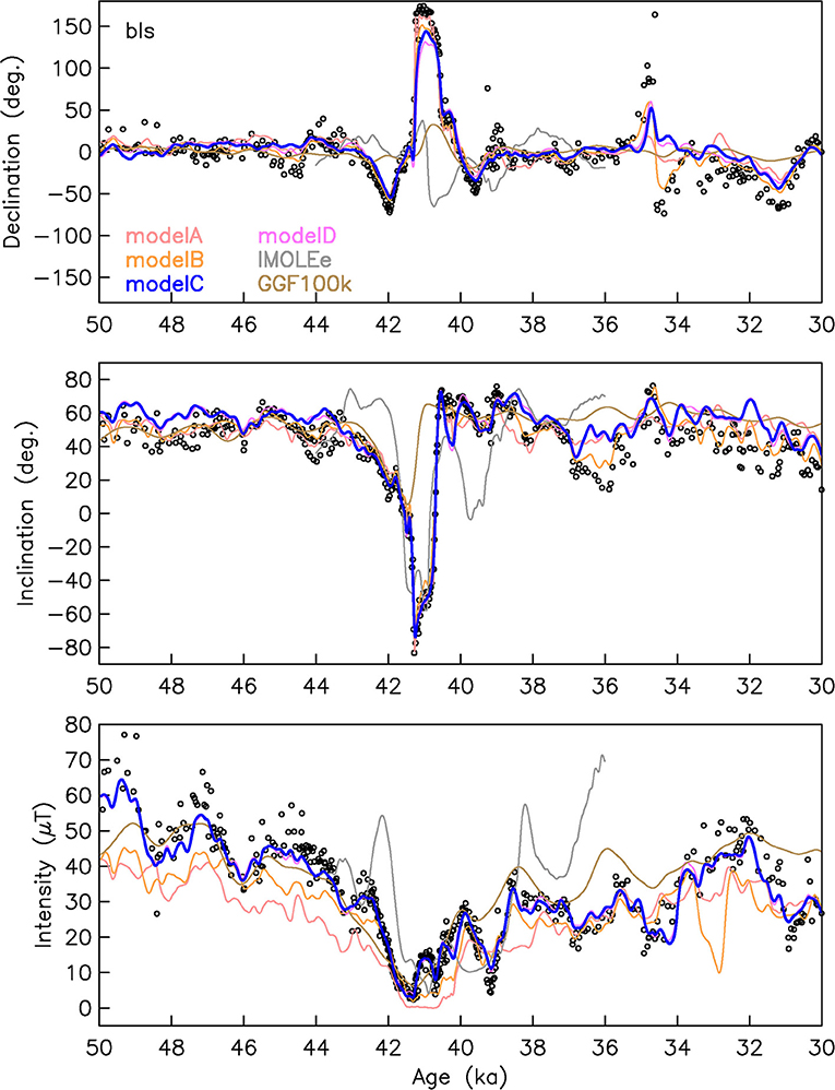
Figure 2. Comparison of the six model predictions (colored lines) to the Black Sea record (black circles) (Nowaczyk et al., 2012, 2013) (c.f. Figure 1 and Table S1) for field components declination, inclination and RPI from top to bottom. Model C (LSMOD.2) is our preferred model.

Examples, such as GAR or PM2 (Figures S7E,H) where in particular the intensity signals show little similarity to model predictions, even when the data were included (model A), justify rejection based on their inconsistency. Examples like ORP or SO1 (Figures S7G,K) justify some age adjustment, as their signals appear similar to the model predictions, but offset in time.

However, it is also obvious that all models, including our preferred model, fail to fit some variations in the data series and may underestimate the full amplitude of the excursion directional swing. This is seen, e.g., in Figure 2 for declination around 33 ka, inclination around 36 and 32 ka and intensity around 49 and 47 ka and many more examples are found in Figure S7. The global regularization smoothes the models too strongly in places in order to avoid spurious structure in other areas. Nevertheless, the regionally organized representative examples in Figure S7 also show that our preferred model does not miss strong directional changes, in particular indications of the Mono Lake excursion, completely.

4.2. Dipole Evolution

In Figure 3 we show the dipole evolution as predicted by the different models and the globally averaged paleo-secular variation (PSV) index $\overline{P_i}$ (Panovska and Constable, 2017) as a measure of overall field variability. The $\overline{P_i}$ global average has been determined based on the model predictions from an equal area global grid based on 1x1° distance at the equator.

FIGURE 3

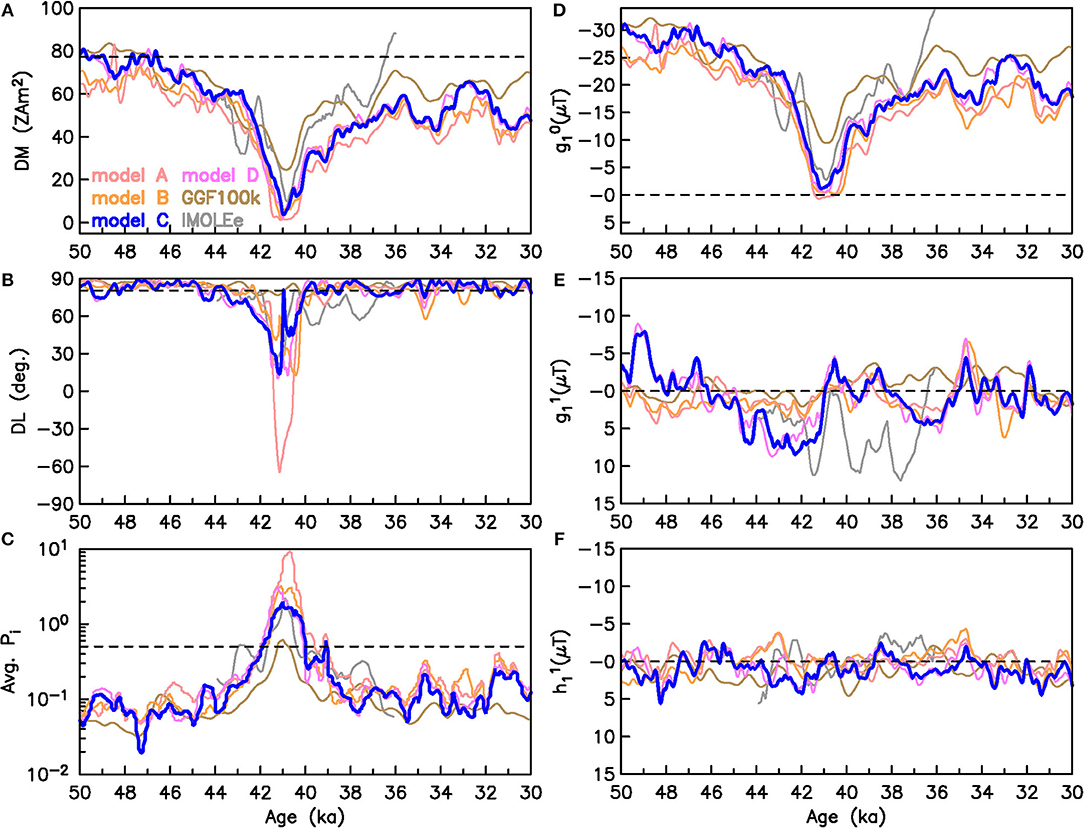
Figure 3. Comparison of the six models in terms of (A) dipole moment (DM), (B) dipole latitude (DL), (C) PSV index P_i, and the three SH dipole coefficients (D–F) at Earth's surface. Dashed lines indicate present day values in (A) and (B), 0.5 suggested as limit for excursional behavior (Panovska and Constable, 2017) in (C) and zero in (D), (E), (F). Model C (LSMOD.2) is our preferred model.

All models show broadly the same DM evolution with a clear, extreme minimum roughly between 43 and 38 ka (Figure 3A), during which the maximum dipole tilt (minimum dipole latitude, Figure 3B) reaches quite different values, though. The latter is not surprising as small differences in equatorial dipole components can have a large effect on dipole tilt when axial and equatorial dipole contributions are of similar magnitude. By definition dipole tilt has little physical meaning when the field is not dipole dominated. IMOLEe and GGF100k have somewhat higher DM due to their different methods of RPI scaling, and the stronger temporal regularization in the case of GGF100k. All other models have minimum DM values below 4 ZAm², and even below 2 ZAm² in models A, B, and D (Table S5), during the Laschamp excursion. The minimum is reached between 41.55 and 40.65 ka, depending on the model. The DM minimum for the Laschamp excursion is broadest for model A, where regionally inconsistent records have been included. Model A therefore produces a global dipole moment that is low for longer than in any of the other models, in particular compared with those where the ages of the Laschamp intensity minimum have less spread (models C and D). Minimum DM values are notably higher during the Mono Lake event, staying above 40 ZAm² in nearly all models (except A). Actually, two similar minima are observed, around ~34 and ~31 ka.

The maximum DM of the models is in the range of 20th century values of ~80 ZAm² (Table S5). However, in all models spanning the 20 kyr interval, the DM does not recover to its pre-Laschamp strength after the excursion. This is accompanied by slightly larger dipole tilt variations than prior to the Laschamp. This is a natural result if the axial dipole contribution (${\text{g}}_1^0$) is weaker but equatorial dipole contributions (${\text{g}}_1^1$, ${\text{h}}_1^1$) stay about the same (Figures 3D–F). The precursory minimum to the Laschamp excursion at about 43 ka found in IMOLEe is not present in any of the models containing more data. Variable small short-term DM minima around 48 and 46 ka accompany surface field intensity structures resembling the present-day South Atlantic Anomaly (SAA) as observed by Brown et al. (2018). A similar structure is also clearly seen in GGF100k at around 46 ka.

4.3. Spherical Harmonic Spectral Power

Time averaged spectral main field power is similar in most of the models up to SH degree five, as shown in Figure 4A. These spectra are averaged over the same time interval as IMOLEe (44 to 36 ka), which is the model of shortest duration. The spectra are further compared to the 400 yr average of gufm1 (Jackson et al., 2000), as a representation of a medium resolution historical to present-day field model. The dipole power of the Laschamp excursion models is lower than of gufm1, as expected, but similar values are found for degrees two to five. The averaged IMOLEe has higher quadrupole and octupole power than the other models, but comparable in degrees four and five. This is due to the sparser data distribution and is not caused by the truncation at SH degree five. We find a similar effect for our test model reconstructed from the 5 IMOLEe records, which is expanded to SH degree 10 (Figure S3C): there, less data are more easily fit by low SH degree field structures, whereas a larger and more diverse data set (model A) requires more power in higher (and not fully resolved) SH degrees. The low degree power of the spectra of models A to D is also controlled by our constraint of an approximately white spectrum for low degrees with stronger damping of higher degrees. This additional constraint differs from GGF100k, where the regularization strength is chosen as the knee of the trade-off between model complexity and its fit to the data.

FIGURE 4

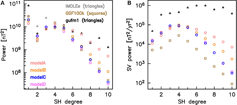
Figure 4. Power spectra at the CMB for (A) the time-averaged field and (B) its secular variation of the six models. All averages are calculated over 44–36 ka. Model C (LSMOD.2) is our preferred model. The 400 years average spectra of the historical model gufm1 are shown for comparison.

The time-averaged SV power spectra (Figure 4B) demonstrate that models A to D all have comparable temporal variability. The spectral SV power is lower than of gufm1, indicating that the field might have varied faster also during the excursion than the models predict. GGF100k has the lowest temporal resolution. The model based on the largest amount of data (model A) requires the highest variability in small spatial scales. When the Laschamp excursion signals are regionally or globally temporally aligned (models C and D) less small scale spatial structure and lower temporal variability are required to fit the data to similar levels.

Some spectral power characteristics at the CMB over time and relations thereof are shown in Figure 5 and Figure S8, including quantities suggested as useful for assessing the Earth-like nature of geodynamo simulations by Christensen et al. (2010). These are relative axial dipole power given by the ratio of power in axial dipole (AD) to non-axial-dipole (NAD) (Figure S8A), i.e., to all the rest, and two measures of symmetry. Equatorial symmetry is expressed by the power in odd (O, equatorially antisymmetric) to even (E, equatorially symmetric) coefficients, with odd and even referring to the difference between SH degree and order (l−m) (Figure S8D). The strongly dominating degree l = 1 is omitted. Axisymmetry or zonality is expressed by the power in zonal (Z, m = 0) to non-zonal (NZ, all the rest) coefficients, again omitting degree l = 1 (Figure S8B). Minimum, maximum and arithmetic mean values of the ratios are listed in Table S5.

FIGURE 5

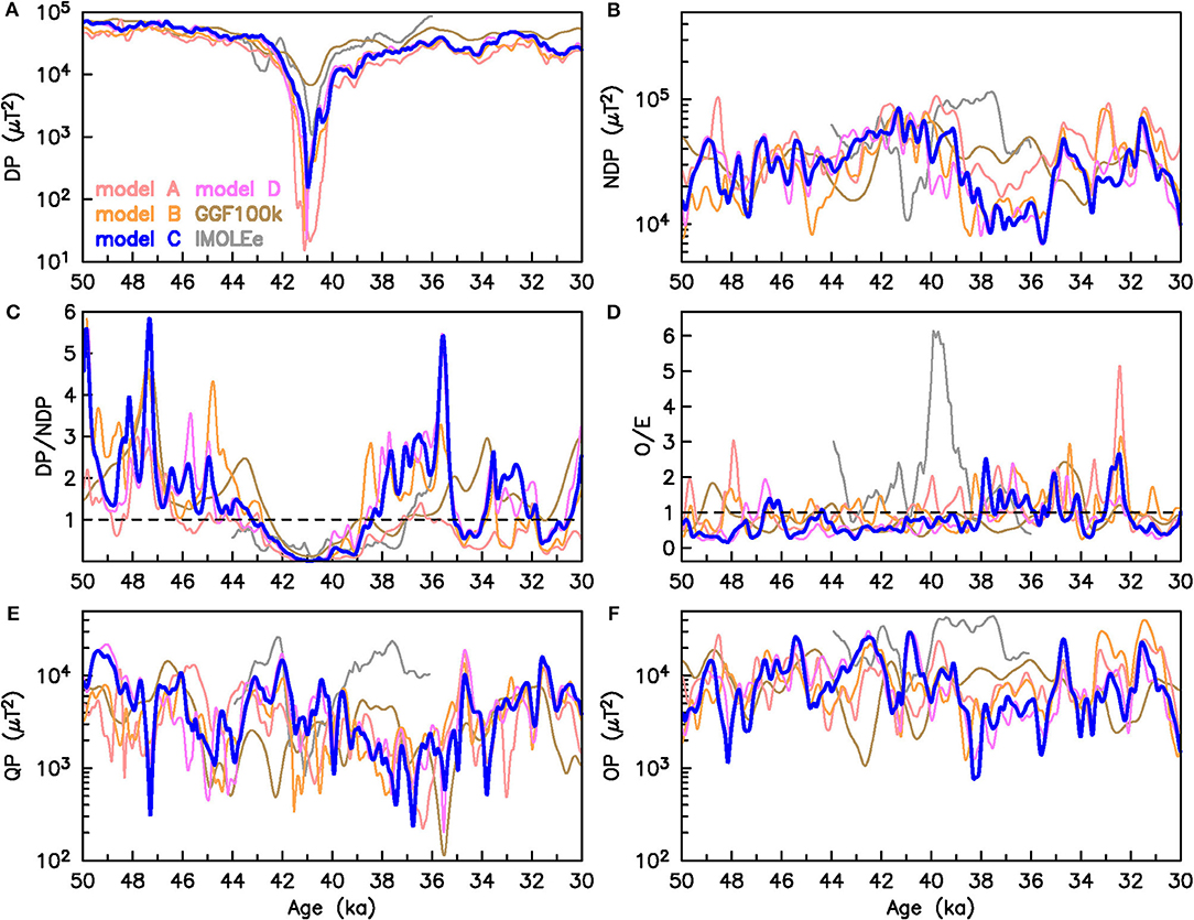
Figure 5. Comparison of various measures of geomagnetic field behavior at the CMB for the six models. (A) Dipole power (DP), (B) Non-dipole power (NDP), relations of (C) power in dipole to non-dipole terms and (D) in odd (O) to even (E) SH terms, respectively, (E) Quadrupole power (QP), and (F) Octupole power (OP). Model C (LSMOD.2) is our preferred model.

The characteristics of models A to D are quite different from IMOLEe in many respects (Figures 5B,D–F). We attribute this to improved data coverage (see section 2). A broad agreement with GGF100k, with its similar data basis, is evident in various quantities over large parts of the time interval.

Unlike IMOLEe, none of the other models suggests that non-dipole power (NDP, Figure 5B) decreases along with dipole power (DP, Figure 5A) during the Laschamp excursion. On the contrary, several models have a slight increase in NDP around the excursion time. Except for models A and GGF100k, where no data selection or age adjustment for regional consistency have been done, the new models have low NDP between ~39 and ~36 ka. This is reflected in relatively high DP/NDP and AD/NAD ratios (Figure 5C and Figure S8A), but these vary notably in all models, in particular while DP is high before the Laschamp excursion. The similarity between DP/NDP (Figure 5C), and AD/NAD (Figure S8A) indicates that there is no strong influence of equatorial dipole components, or of significant dipole tilt during times of clearly dipole dominated field. During the Laschamp excursion the ratios become close to zero due to the low DP. As noted by Christensen et al. (2010), the AD/NAD ratio cannot be directly compared to present-day values due to the limited resolution of paleomagnetic models (and the same is true for DP/NDP).

Quadrupole and octupole power (Figures 5E,F) in particular vary notably and rather rapidly over time, with only very few of these variations appearing consistent (within some uncertainty) in phase and amplitude in several of the models. The spectral power distribution clearly depends strongly on data distribution and weighting and must not be over-interpreted.

The average O/E ratios of the models are similar to the historical field [0.84 to 1.42 (Christensen et al., 2010)], but vary over a larger range (Table S5). The same is true for zonality. The strong increase of equatorial antisymmetry during the Laschamp excursion shown by IMOLEe is not reproduced in any other model, but several of them show a short time peak of O/E at about 33 ka (Figure 5D). In general variations in equatorial symmetry (Figure 5D) and zonality (Figure S8B) ratios appear partly consistent among models in a similar way as quadrupole and octupole power.

4.4. Global Excursion Duration

Defining the beginning and end of an excursion is not straightforward. The excursion process in the core manifests itself in globally non-uniform directional and intensity variations at Earth's surface. This makes defining a cut-off for the beginning and end of an excursion problematic when using individual surface observations. Furthermore, as will be seen in the following, all our models suggest that local changes in direction and intensity are shorter in duration than the overall duration of the underlying excursion process. We consider three parameters that might serve to define the global excursion duration: (1) the global average $\overline{P_i}$ at Earth's surface; (2) the point at which the power spectrum becomes flat at the CMB and (3) DP/NDP at the CMB.

Panovska and Constable (2017) suggested P_i ≥0.5 as representative of excursional field behavior. This value was calculated using the commonly used 45° VGP latitude cut-off for excursions and a virtual (axial) dipole moment (VDM or VADM) of about half the present day field (40 ZAm²). We use the times when $\overline{P_i}$ exceeds 0.5 to define the start and end of the surface field observations associated with the Laschamp excursion. The onset/cessation times and the duration constrained by P_i are given in Table 2 for all six models. For the four models constructed as part of this study, the surface field enters an excursional state around 42 ka and exits around 40 ka (although there is 500 years difference between model A and model C). If we take the model C duration as our best estimate, the major surface field directional and intensity changes associated with the Laschamp excursion occur within a 1.8 ka window.

TABLE 2

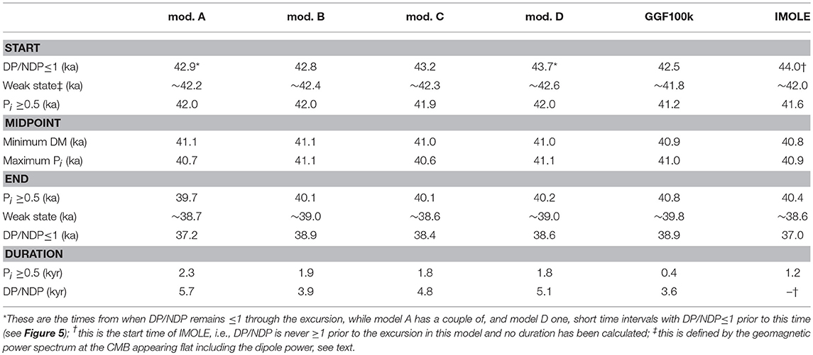
Table 2. Global age (start, mid-point, end) and duration of the Laschamp excursion in the six models considered in this study.

To investigate the duration of the underlying excursion process we take two approaches. The first is to define an excursion state following the suggestion of Brown et al. (2018). They proposed two mean states of the geomagnetic field: a dipole dominated state vs. a state where the dipole power is comparable to the power in the individual higher order SH degrees at the CMB. The initiation of the Laschamp excursion would therefore not be expected to occur before the dipole power has reduced to a similar level of power as in the individual non-dipole components of the field. Estimates of the beginning and end of this state according to visual inspection of the model spectra are included in Table 2.

A slightly different, but more easily quantifiable criterion is DP/NDP = 1, where non-dipole power is summed up. This measure depends on model resolution or SH truncation degree if the main field power spectrum is white for the non-dipole field at the CMB. With the limited model resolution to approximately degree 5 the ages according to this criterion differ by a couple of centuries from the Brown et al. (2018) criterion (Table 2). A justification for why DP/NDP up to SH degree 5 seems an empirically suitable criterion is seen in Figure S6: the input data from a numerical dynamo simulation with white CMB power spectrum are fit closely at Earth's surface (Figure S6A) by a model of effective resolution no higher than degree 5 to 6 (Figure S6C). Higher degree contributions to surface field variations are minor due to mantle filtering (the temporal variations could not be fit so closely if they were too small scale to be resolved spatially by the model).

All models indicate that the field enters the weak state at about 42 ka or a few centuries earlier, and the Laschamp excursion begins to show at the surface about 600 years later, with a duration of ~2 kyrs. Only IMOLEe and the more strongly smoothed GGF100k show clearly shorter durations of 1.2 and 0.4 kyrs, respectively. The global excursion midpoint according either to minimum DM or maximum $\overline{P_i}$ lies between 41.1 and 40.6 ka in the different models. Highest $\overline{P_i}$ values are shown by model A with the largest amount of most diverse data.

In all of our models, the axial dipole does not fully recover to pre-Laschamp strength in the studied time interval. The field seems to remain close to the weaker state, allowing the occurrence of the Mono Lake excursion, although intervals of dipole dominance at the CMB are also seen (c.f. Figure 5C). Note that our study cannot inform whether globally seen excursions are in general followed by the field remaining in the weak state for some time or whether prompt full dipole recovery is possible as well. The Mono Lake excursion does not exceed the global 0.5 $\overline{P_i}$ threshold in any of the models.

4.5. VGP Paths and Regional Differences

VGP paths have been widely used to study transitional field behavior from individual sites (e.g., Hoffman, 1981; Laj, 1991; Love, 1998; Laj and Channell, 2015). We calculated 1667 VGP paths from each of the models evenly distributed over the globe (as a sphere on a 5° grid), each consisting of 101 values in 20 years steps from 43–39 ka BP for the Laschamp, and from 36–30 ka BP for the Mono Lake excursion. Moreover, we determined the minimum values and ages of VADM and VGP latitude, and the maximum values of P_i within these time intervals from global 1x1° grids, and also the duration of the excursions according to P_i > 0.5 Results for our preferred model C (LSMOD.2) are shown in Figures 6, 7, 8. The following discussion focuses on these results, which are broadly seen in all models. Noteworthy differences among models are pointed out and several comparison plots with the other models are given in Figures S9–S15.

FIGURE 6

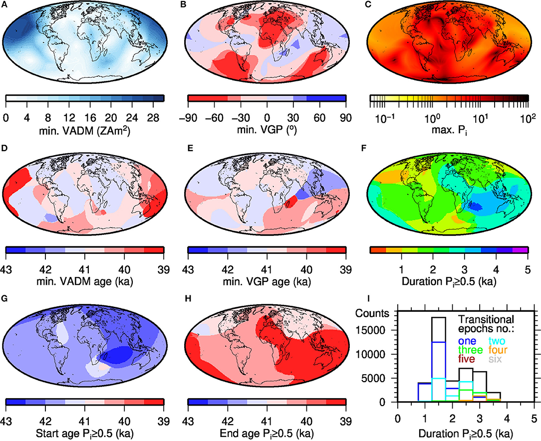
Figure 6. Minimum VADM (A), VGP (B, note the non-linear color scale) and maximum P_i (C) reached in different areas (at different times) during the Laschamp excursion; ages when minimum VADM (D) and VGP (E) values are reached; (F) regional duration of the excursion according to P_i ≥0.5 and earliest (G) and latest (H) age of P_i = 0.5; and histograms of duration of the Laschamp excursion in 500 years bins (I) according to earliest and latest P_i ≥0.5 occurrence (black). Colored lines indicate whether P_i ≥0.5 for the whole duration or whether this time was split into two (cyan), three (green), four (orange), five (brown), or six (gray) intervals between which P_i < 0.5. All results are from our preferred model C (LSMOD.2).

FIGURE 7

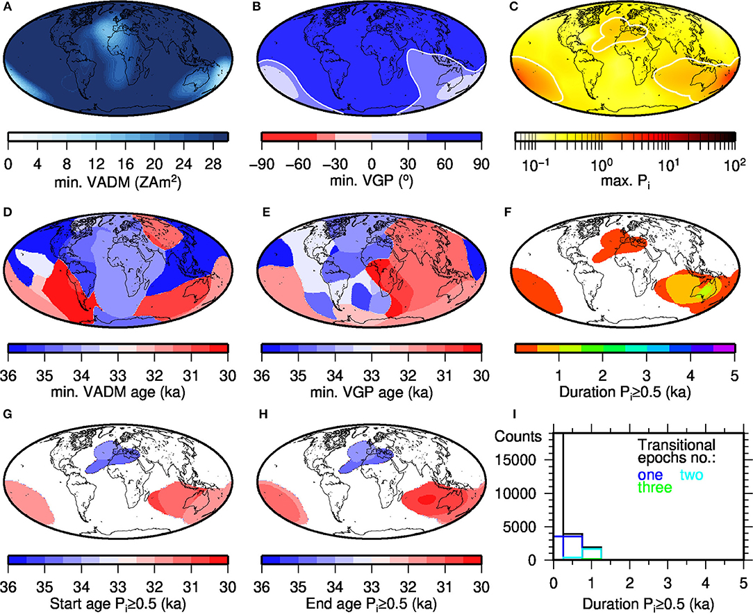
Figure 7. Minimum VADM (A), VGP (B, note the non-linear color scale) and maximum P_i (C) reached in different areas (at different times) during the Mono Lake excursion; ages where minimum VADM (D) and VGP (E) values are reached; (F) regional duration of the excursion according to P_i ≥0.5 and earliest (G) and latest (H) age of P_i = 0.5 (P_i does not exceed 0.5 in white areas); and histograms of duration of the Mono Lake excursion in 500 years bins (I) according to earliest and latest P_i ≥0.5 occurrence (black). Colored lines indicate whether P_i ≥0.5 for the whole duration or whether this time was split into two (cyan) intervals between which P_i < 0.5. All results are from our preferred model C (LSMOD.2).

FIGURE 8

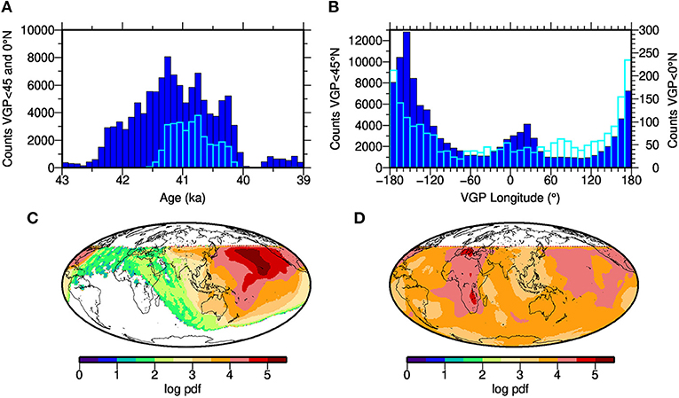
Figure 8. VGP statistics during the Laschamp excursion from model C (LSMOD.2), determined from an equal area grid defined by 5° latitude by 5° longitude at the equator. (A) Temporal distribution of all VGPs ≤ 45°N (blue) and ≤ 0°N (cyan) between 43 and 39 ka in 100 yr bins. (B) Distribution of all VGPs ≤ 45°N (blue, left ordinate) and VGPs crossing the equator (cyan, right ordinate) between 43 and 39 ka by longitude in 10° bins. (C) Global density distribution of all VGPs ≤ 45°N from 42.2 to 41.2 ka and (D) from 41.2 to 40.2 ka. The logarithms of the determined smoothed probability density functions (pdf) are shown. White areas <45°N have zero probability density, and VGP latitudes >45°N were not plotted (white) to avoid the strong dominance by high latitude VGPs in the density distribution even during the excursion.

For the Laschamp we first note that in most of the models VGP latitudes below 45°N, commonly considered as transitional, are observed all over the globe (Table S6 and Figure S9). The exceptions are GGF100k, and four small regions in model A (2% of the sites). The reason that only 21% of the records reach transitional VGPs in GGF100k lies in its lower temporal resolution compared with the dedicated excursion models. The occurrence of small regions with no transitional VGPs in model A is due to the higher spatial resolution that allows larger regional differences in field variations. Between 68 and 76% of VGP paths cross the equator in our new models, and 18 to 36% reach 45°S. These numbers are much smaller for IMOLEe (a result of insufficient data coverage) and GGF100k (owing to stronger smoothing). Our new models agree partly on the locations which give equatorial and southern hemisphere VGPs (Figure S9). In all these cases the areas that predict southernmost VGPs include South America and surroundings, eastern Australia and parts of the southern Indian Ocean, and European to western Asian regions (Figure 6B and Figure S9). These areas generally coincide with the areas of weakest intensity (Figure 6A and Figure S9). All models (again with the exception of GGF100k) indicate that the PSV index exceeds 0.5 all over the globe for some time during the Laschamp (Figure 6C and Figure S9). The highest values, indicating strongest field variability, appear in the Atlantic and parts of the Indian Ocean regions. The lowest values are found in the Pacific. The distribution of P_i values in IMOLEe coincides with the underlying data distribution (compare Figure S9 and Figure 1), and we attribute the lower PSV activity in and around South America to a lack of data.

The minima of VADMs (Figure 6D), as well as VGP latitudes (Figure 6E), do not occur at the same time all over the globe. For instance, early occurrences of both VADM and VGP latitude minima are found in the South Atlantic region, whereas VADM minima are found later in the Australian region. Although such time differences are seen for all models, the specific occurrence times are different for each of the models (Figure S11). This may partly be due to some of the time series having more than one intensity or VGP low, so that the absolute minimum might not always be the best indicator for the excursion midpoint at an individual site (see Figure S7). It also reflects the assumptions made about alignments in the regional excursion signals in the different data sets. Thus, the spread is smaller in model D (strong alignment) than model A and GGF100k (no alignment). The late occurrence (~39 ka) of VADM minimum in the Pacific area in model C is somewhat surprising. Considering the earliest and latest occurrence of P_i ≥0.5, the regional duration of the Laschamp mostly ranges between 1 and 4 kyr. It is mostly shorter in GGF100k and with small areas with durations up to 5 kyr in models A and IMOLEe (Table S7). However, in regions with long excursion durations P_i does not always remain above 0.5 for the duration of the excursion. Brief epochs with P_i < 0.5 give the appearance of two, three or even more consecutive transitional intervals (Figure 6I and Figure S13). The onset and end times of regional excursions based on P_i > 0.5 vary regionally by more than 1 kyr (Figures 6G,H). Our models consistently suggest that the Laschamp begins across the Indian Ocean and has the longest duration in that area (Figure S13).

During the Mono Lake excursion (not covered by IMOLEe), none of the models predicts VGP paths that reach equatorial latitudes (except for a very small region in the southern Pacific in model A). On the contrary, even transitional VGP latitudes (<45°N) are only obtained from a few areas of the world in all models (4 to 31% of the VGP paths), mainly from the southern Pacific (Figure 7B and Figure S10). This is also nearly the only region where P_i exceeds 0.5 (Figure 7). Frequent regional excursion signals occur most often in model A between 35.1 ka and the end of the studied time interval, and less often in the strongly age-aligned model D (Figure S10). The minimum VADM does not fall below ~30 ZAm² during the Mono Lake excursion in most regions (Figure 7A and Figure S10). The ages of minimum VADM and VGP latitude values are variable from 36–30 ka (Figures 7D,E, and Figure S10). In most models they appear at about 34 ka in the Atlantic and surrounding areas and at about 31 ka around Australia (Figures 7F–H). The maximum regional duration of both of these events is below 1.5 kyr in our preferred model C, with a maximum of two distinct transitional epochs (Figures 7F,I). Model A has several short intervals with regional P_i > 0.5 in the southern hemisphere (Figure S10). The models suggest that more than one regional “Mono Lake” excursion have occurred in the time interval 36–30 kyr.

The longitudinal distribution of VGP paths is uneven during the Laschamp excursion in all models. In Figure 8 and Figure S14 we show the longitudinal distribution of all VGPs that fall between 45°N and 45°S, and from those crossing the equator, from the calculated grid paths. We see from Figure 8A that most transitional VGPs are reached between 42 and 40 ka (the interval used for Figure S14). Both the longitudinal distributions of the 45°N-45°S VGPs and the equator crossings have similar maxima and minima and suggest that the VGPs have a preference for longitudes between roughly 160°E and 160°W. Another grouping appears non-uniform across the models' distributions: between 20 and 50°W in models A and B, but around 20°E in models C, D and IMOLEe. Figures 8C,D illustrate through VGP density plots for the earlier and later half of the Laschamp (here taken as 42.2–41.2 and 41.2–40.2 ka) that several VGPs tend to a clockwise loop, going south over the Pacific and returning north over Africa. This is reminiscent of a loop that was described for a compilation of individual data records by Laj et al. (2006); Laj and Channell (2015). The few VGP paths that cross 45°N during the Mono Lake excursion fall around 40°E in models A and B and closer to 0° longitude in models C and D (Figure S15).

4.6. Field Morphology

Using our SH models to map the field at Earth's surface or the CMB can give a general idea about field morphology, but small scale structures should be interpreted with care. For example, intensity minima, that accompany reverse flux patches at the CMB, and which resemble the present day SAA, appear in all models around 46 ka (Figure S16), but vary in strength and their exact location.

Figure 9 depicts surface field intensity, VGP latitude and radial field (B_r) at the CMB for the beginning, middle and end of the Laschamp excursion (defined by $\overline{P_i}$ exceeding 0.5) and for 34.7 ka, the potential middle of one of the Mono Lake excursions from our preferred model. The following discussion is based mainly on these results, with differences among models noted and illustrated by model comparisons in Figures S17–S21. Due to the age adjustments applied to the data sets used for several of the models, comparing field morphologies at slightly different times according to this criterion is more reasonable and gives more similar results than mapping all models for exactly the same ages.

FIGURE 9

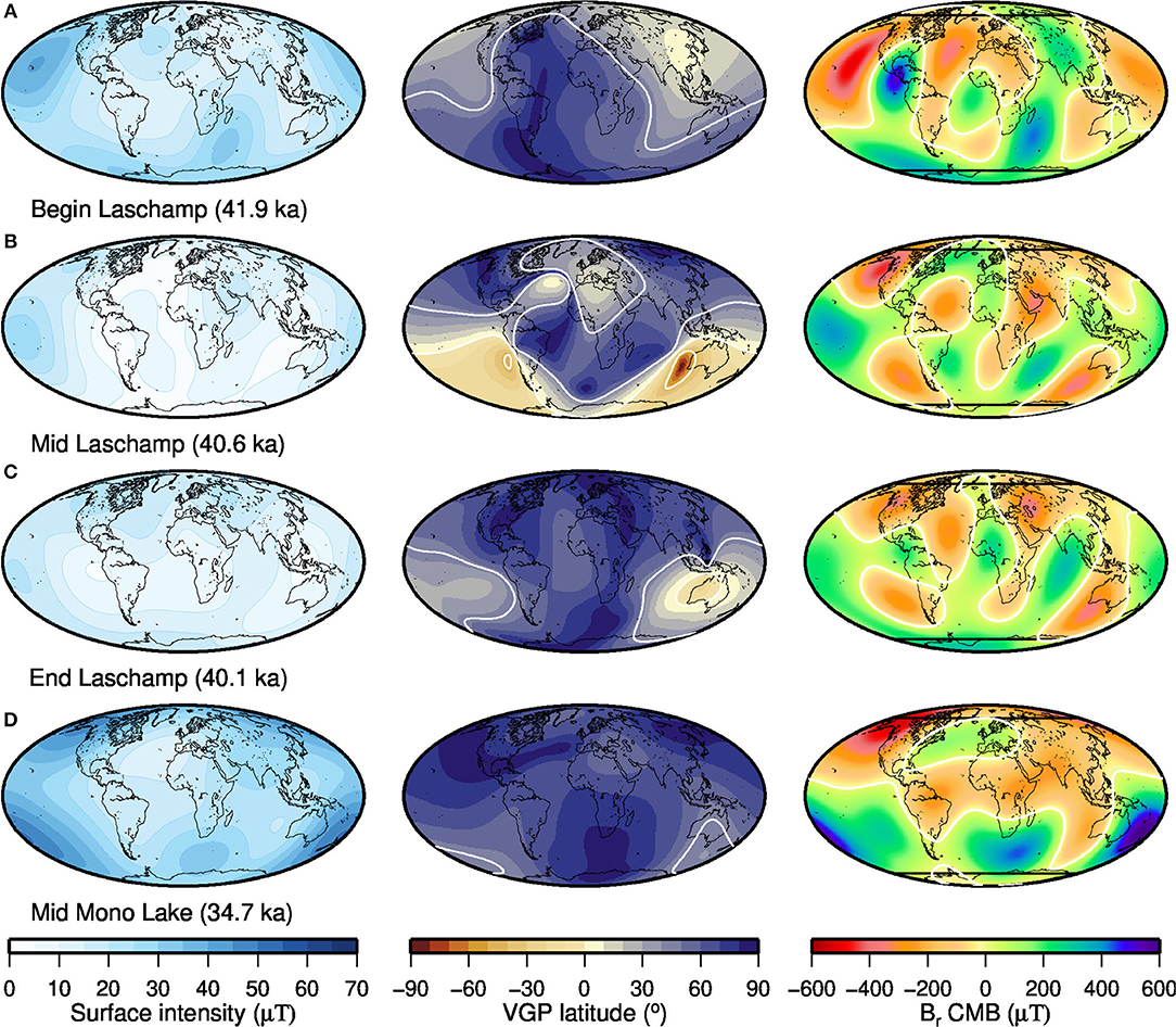
Figure 9. Field morphology at (A) beginning, (B) middle, (C) end of the Laschamp excursion, and (D) the middle of the Mono Lake excursion according to maximum P_i values and model C (LSMOD.2). Field intensity at the Earth's surface (left), VGP latitude distribution (middle) and radial field at the CMB (right). White lines in the middle and right panels indicate 45° and 0 μT, respectively. Black lines in the right panels indicate the tangent cylinder.

The excursion starts with field strength getting weak in several parts of the world, associated with reverse flux patches appearing in northern to central American, Asian and southern Indian Ocean regions. Excursional directions with VGP latitudes <45°N occur in similar areas. (Figure 9A and Figure S17). Intensity is weak all over the globe in the middle of the excursion (Figure 9B), with minimum values at the Earth's surface <1μT in all cases, as low as 0.03 μT in model A and 0.12 μT in preferred model C (Figure S18). Most of the models suggest that intensity gets weakest over the Atlantic and parts of the southern Indian Ocean and remains slightly stronger over the western Pacific. However, flux patterns at the CMB appear partly contradictory among the models during the main excursion phase. The same is true for VGP latitudes predicted by the various models for different parts of the world at this time, but these vary rapidly. Differences in flux distribution at the CMB and VGP latitude distribution from the different models remain toward the end of the excursion and for some time afterwards (Figure 9C and Figure S19). Nevertheless, nearly all models show notable amounts of reverse flux inside the tangent cylinder (TC) in both hemispheres during the main phase of the Laschamp excursion, partly seen in Figure 9B and Figure S18.

Maps of the middle of the Mono Lake excursion according to maximum $\overline{P_i}$ (Figure S20) show stronger dipolarity, with weak surface intensity and some reverse flux at the CMB from the Americas to Asia and Australia, but not over the Pacific. The maximum $\overline{P_i}$ of the Mono Lake excursion is found at the same time (34.7 ka) in most models, while the minimum DM occurred several centuries later. None of the models predict transitional VGP directions at that time, but the flux distribution at the CMB has some additional reverse flux in the Pacific region (Figure S21). The amount of reverse flux seen inside the TC during the Mono Lake excursion appears less than during the Laschamp, but it varies notably among the models.

5. Discussion of Robust Excursion Features and Geophysical Implications

The comparison of several features from a range of global SH models in section 4 indicates both robust and less certain global characteristics of the Laschamp and Mono Lake excursions. We start this discussion by focussing on the differences seen in our models before summarizing the observations that are consistent in all models.

The results from the previously published IMOLEe model deviate in several aspects from the new models due to its much more limited data coverage (Figure 1). Several sediment records that we used were not published at the time IMOLEe was created (Table S1). Moreover, we followed a less strict data selection strategy than Leonhardt et al. (2009). In particular we included also incomplete vector records. For any global field model we face a trade-off between good data coverage and quality selection criteria, and subjective choices have to be made about the data to include in the modeling. We currently do not have a complete understanding of the reliability of all published paleomagnetic data. Despite a significant amount of research and progress in the field, several aspects of the remanence acquisition process that may affect paleomagnetic sediment data quality remain hard to assess objectively (see, e.g., Roberts et al., 2013; Tauxe and Yamazaki, 2015; Chang et al., 2016). Prior data selection is largely based on which records have “reasonable” or “unreasonable” paleomagnetic variations through time and whether a collection of records are regionally consistent. Such a selection makes implicit assumptions about the temporal and spatial complexity of the field. The modeling method can discriminate between consistent and inconsistent data to a certain amount (section 4.1 and Figure S7) under the regularization constraints. These constraints are also based on assumptions about past field characteristics and assumed to be physically reasonable. SH models, such as ours represent smoothed field behavior. Rapid field changes may be distorted and field structure may lack in them. This applies in particular to regions where input data are strongly smoothed representations of geomagnetic variation, e.g., when u-channels were used (as is the case for more than half of our records, see Table S1) or sedimentation rate was low (Roberts and Winklhofer, 2004; Philippe et al., 2018). Our new models and GGF100k use a similar data compilation and modeling method, but employ different data treatments. Their large scale characteristics appear broadly similar when considering that GGF100k is more strongly regularized, particularly in time. This indicates that robust information can be obtained from presently available paleomagnetic data.

Uncertainties in sediment chronologies remain a source of ambiguity when reconstructing past field variations. The similarity in overall rms misfit of all our new models indicates that it is possible to fit many variations on their original time scales without the need for strong paleomagnetic age alignment (Table S4). Age offsets seen in visual comparisons between input data and model output indicate errors in the chronologies of some records. However, an overall slightly worse fit to directional data going along with a better fit to intensity data in the more strongly aligned models C and D leave details of the question of contemporaneity of the excursion signal in different locations open (section 4.1). Our new models suggest that both minimum VADMs (intensities) and VGP latitudes might be offset regionally by up to 3 kyr within the time interval 42.13 ka to 38.95 ka (Figure 6).

The similar overall fit to the data is obtained with different SH spectral power distributions (section 4.3 and Figure 4). The less distributed and more aligned the data are (models C and D), the more power is found in the longer ND wavelengths (quadrupole and octupole) and their temporal variability, and globally the excursion appears a few centuries shorter at Earth's surface. To fit the data similarly well, the models based on more individual and less chronologically aligned data require more power and variability in smaller-scale structure, but still well below the values found in the present-day field. The 1.8 kyr global surface field duration of the Laschamp excursion predicted by age-aligned models (C and D) may be considered a lower bound, and the longest value we found is 2.3 kyr (model A). The regionally predicted durations from our models on full global grids based on P_i are in general in good agreement with the durations from 0.35 to 3.10 kyr, with an average of 1.3 kyr, found by Panovska et al. (2018a) directly in their global sediment data compilation. We found only a few areas of longer and shorter duration and only a slight dependence of the maximum regional dependence on the degree of age alignment in the underlying data.

Based on individual records it has been suggested that VGPs might follow preferred longitudinal paths during excursions and reversals, related to non-axial-dipole components of the field. For the Laschamp excursion, Laj et al. (2006) [updated by Laj and Channell (2015)] found a simple clockwise VGP loop passing south through the western Pacific and back north through Africa, which they attributed to a substantial influence from equatorial dipole contributions and a reduced non-dipole field during the excursion. Influence from lowermost mantle conditions on the geodynamo could explain persistent non-axial-dipole contributions causing preferred VGP paths (Laj, 1991; Gubbins and Coe, 1993; Gubbins, 1994). However, the existence of preferred VGP paths is under debate (see, e.g., Roberts, 2008; Laj and Channell, 2015; Valet and Fournier, 2016). A global evaluation of VGP paths suggests a longitudinally uneven distribution of VGPs in all our models (section 4.5). Although the preferred longitudes vary somewhat among the models depending on data distribution, they roughly agree with those suggested from globally uneven data distributions for both the Laschamp and, in reverse direction, for the Iceland Basin (~190 ka) excursion (see Laj and Channell, 2015). However, there is a large range of VGP locations and not all VGP paths follow the preferred paths. They do not support the interpretation of a rotating dipole as suggested by Laj et al. (2006), and moreover, none of our models has the reduced non-dipole contributions during the excursion that is required in that scenario.

Some other characteristics are found in all our models and can be considered reliably resolved given the presently available data. There are clear differences between the Laschamp and Mono Lake excursions. Most of our input data cover both time intervals, so this should not be an artifact.

The Laschamp excursion is characterized by a significant drop in axial dipole power to around 0 for an interval between a few centuries and ~ 1 kyr, which results in low intensity (or VADM) values, transitional VGPs and P_i > 0.5 all over the globe within this time (see sections 4.2, 4.6). Equatorial dipole contributions and ND field do not seem to contribute to the development of the excursion, although the ND field might increase during the excursion (see sections 4.2, 4.3). This result is in contrast to the earlier IMOLEe model, where the ND energy decreased along with the dipole energy. It agrees with a conclusion by Lund (2018) from his statistical analysis of PSV records from three globally distributed regions, that globally diminished field intensity is the main factor leading to an excursion.

The NAD field variations determine the location and timing of absolute VADM and VGP latitude minima, PSV activity and field morphology at the CMB. The latter are not robustly resolved, but some features are common to all of our models (see sections 4.5, 4.6). PSV activity during the Laschamp is stronger in the Atlantic and Indian Oceans than the Pacific Ocean, and in the Southern rather than the Northern hemisphere. Similar differences have been found on time scales from the present day (Holme et al., 2011), over recent centuries (Jackson et al., 2000), the Holocene (Constable et al., 2016), the past 100 ka (Panovska et al., 2018a), to millions of years [e.g., see also Panovska and Constable (2017), Cromwell et al. (2018)]. This morphological agreement in field variability during the Laschamp excursion and over a large range of time scales may be a further indication that NAD variations do not change fundamentally during the excursion and may support the hypotheses that excursions are part of normal SV, occurring during a weaker base state of the field with strong axial dipole variations (Brown et al., 2018).

In all of our models the axial dipole (and consequently also the DM) does not recover to its pre-Laschamp strength after the excursion (section 4.2). This weaker axial dipole phase lasts from 39 ka to the end of the models at 30 ka, while NDP is similar to other times from 36 to 30 ka (and weaker from 39 to 36 ka). Although a persistence of the field in or close to the weak state probably leads to the Mono Lake excursion, the axial dipole does not decrease as strongly during this event than during the Laschamp. In fact all models suggest two epochs of moderate dipole lows, around 34 and 31 ka (Figure 3). As two lows are also seen in GGF100k and directly in a number of RPI records (Figure S7) the younger low is real and not due to modeling edge-effects near the end of our time interval. Note also that two production rate maxima are found in cosmogenic isotope records at about these times (e.g., Wagner et al., 2000; Adolphi et al., 2018), also indicating two intervals of globally low magnetic field intensity. We find transitional VGPs and P_i ≥0.5 in only a few regions and not globally during these two times (see sections 4.5, 4.6), which we propose to be two separate excursions with non-global directional surface signatures. Our results do not exclude the possibility that some sediment records, and consequently also the models, might lack excursion signals in some areas due to smoothing associated with remanent magnetization acquisition (Roberts and Winklhofer, 2004). However, as our continuous models are based more or less on the same sediment records over both excursions we conclude that the observed differences between the two events are real. They are consistent with the theory that excursions might result (nearly) purely from axial dipole variation, which might vary over a wide range of amplitudes during a weak field state (see also Brown and Korte, 2016).

We now expand the hypothesis by Brown et al. (2018), that the geodynamo has two states, and propose to consider three states based on the studied time interval (Figure 10). The first state, which is similar to the present day field lasts from 50–43 ka. In this state the field is dipole dominated and the axial dipole varies over longer times scales than small scale non-dipole secular variation. A second state is characterized by significant axial dipole field decay to nearly zero or even slightly reversed values. The global field becomes temporally weak and transitional directions are seen across Earth (at regionally slightly different times). Non-dipole secular variation remains generally unchanged and is similar to times when the field is in a non-transitional state, although some energy from the dipole might be transferred into NDP. In the third state, found from ~38 ka to at least the end of our model at 30 ka, non-axial-dipole secular variation is still unchanged, but the axial dipole is at a similar level. The field is not so strongly dipole dominated as in the first state, leading to frequent excursions with only a moderate decay of the axial dipole and regionally confined directional signatures at Earth's surface. Such a field state could also explain the widely spread ages of some excursions at other times, e.g., around the Tianchi/Hilina Pali excursion in the interval 22–17 ka. Ahn et al. (2018) recently suggested that a series of multiple excursion swings might have occurred in this time interval, based on preliminary results from a Korean sediment section. In such a phase, one should be extremely careful in using excursions from individual records as stratigraphic markers across large areas, such as different continents or oceans. Note that our present study cannot inform us whether we should consider reversals as a fourth state, or whether there is no real distinction in the process of the direction of axial dipole recovery in the second state. Wicht and Meduri (2016) found similar behavior in a long numerical dynamo simulation that had phases of high dipole moment with stable polarity and phases of low dipole moment with reversals and excursions. As in our empirical models, the equatorial dipole had a negligible role in the excursions. They found no clear distinction between strong excursions and reversals and attribute the direction of the axial dipole recovery to chance.

FIGURE 10

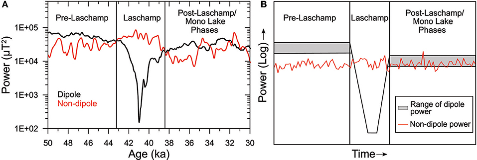
Figure 10. Dipole and non-dipole power evolution at the CMB between 50 and 30 ka from LSMOD.2 (A) and a generalized schematic of three proposed geodynamo states (B). The gray box encapsulates the range of slow dipole power variations. Faster non-dipole power is shown as white noise.

6. Conclusions

We have created a suite of global paleomagnetic field models spanning 50 to 30 ka, including the Laschamp and Mono Lake excursions, from a compilation of 50 published paleomagnetic sediment records and all available volcanic data that we were aware of. Such models have a range of applications, such as predicting the geomagnetic field at any location on Earth, mapping the field and its evolution at the surface and the CMB (allowing inferences about the mechanisms that generate the field), estimating shielding against galactic cosmic rays and solar wind using dipole moment and tilt, and studying spectral power variations to compare with numerical geodynamo simulations. However, variations in assumptions about the quality of the paleomagnetic signal in the sediments and the accuracy of the independent age scales lead to differences in model outputs. We investigated a range of data sets and models, ranging from using all independently dated records with minimum additional assumptions, to data selection based on regional consistency with maximum temporal alignment of the field intensity minimum from all sites.

Several characteristics are found in all models and robustly resolved: (1) clear differences between the Laschamp and Mono Lake excursion; (2) a global duration of the Laschamp of ~2 kyr at Earth's surface and ~5 kyr at the CMB, with (3) a drop of the axial dipole strength close to zero during the Laschamp, and (4) no apparent change in NAD variability with perhaps some increase in overall NAD power. Other features, in particular the distribution of power among different spatial non-dipole scales and details about CMB field morphology depend more strongly on assumptions about the underlying data sets and should be interpreted with care.

We propose (at least) three states of the geodynamo, which are primarily related to the the axial dipole contribution. Secular variation in all other contributions does not seem to change notably across these states. They are (1) a stable, strongly dipole dominated field configuration, found in our study from 50 to 43 ka and similar to the present day, (2) extreme axial dipole decay to a level where the non-dipole field dominates at Earth's surface and transitional field behavior is found all over the globe, as during the Laschamp excursion from ~43 to ~38 ka (which might or might not be a similar state as during the transitional phase of a reversal), and (3) similarly strong axial dipole and NAD field contributions, allowing frequent regionally confined excursion signatures to appear, found in the interval from ~38 to 30 ka. Excursional directions around 34 and 31 ka indicate that the Mono Lake excursion is a series of regionally manifest events rather than one globally seen excursion.

Although we have resolved a number of robust features of the field during excursions, the current underlying data set does not allow us to investigate smaller scale structures of the field at Earth's surface and CMB. Some features of individual records are not fit well by the model, which in general give a smoothed representation of the field. New high-resolution paleomagnetic sediment discrete sample and volcanic data, in particular from hitherto sparsely covered regions, further progress in understanding sediment magnetization acquisition processes and in particular further improvements in dating accuracy for both sediments and volcanic rocks are the required ingredients to resolve more global excursion characteristics robustly.

Moreover, the Laschamp and Mono Lake are only two excursions. Excursions may show a range of behavior depending on the field state. For example, one interesting question is whether the Laschamp is an end member excursion, in the sense of being the most extreme the field can get before a reversal is induced, or whether we can we get excursions that show a substantially reversed axial dipole component. Global investigation of other excursions/reversals and numerical dynamo simulations will allow us to answer these questions in the future.

Author Contributions

The new models were derived in close collaboration between MB, who compiled and processed the data, and MK, who ran the modeling code. MK, MB, and IW designed the tests with synthetic data, using the toy model by MB and numerical dynamo simulation by IW. Data analysis was carried out by MK, and observed results were discussed among all authors, including SP who provided the GGF100k model prior to its publication. MK wrote the initial version of the manuscript that was revised by all authors.

Funding

MB was supported by the Deutsche Forschungsgemeinschaft SPP PlanetMag 1488 project BR4697/1.

Conflict of Interest Statement

The authors declare that the research was conducted in the absence of any commercial or financial relationships that could be construed as a potential conflict of interest.

Acknowledgments

We are grateful to all colleagues who made their paleomagnetic data available for this study, either personally or through data publication or database entries. We thank Sydney R. Gunnarson for her help in data preparation and Catherine G. Constable for sharing her computer code to calculate VGP probability densities. Figures were prepared with the free softwares Generic Mapping Tools (GMT) (Wessel and Smith, 1998) and plotxy by Bob Parker (https://igppweb.ucsd.edu/~parker/Software/).

Supplementary Material

The Supplementary Material for this article can be found online at: https://www.frontiersin.org/articles/10.3389/feart.2019.00086/full#supplementary-material

References

Adolphi, F., Ramsey, C. B., Erhardt, T., Edwards, R. L., Cheng, H., Turney, C. S., et al. (2018). Connecting the Greenland ice-core and U/Th timescales via cosmogenic radionuclides: testing the synchroneity of Dansgaard–Oeschger events. Clim. Past. 14, 1755–1781. doi: 10.5194/cp-14-1755-2018

CrossRef Full Text | Google Scholar

Ahn, H.-S., Sohn, Y. K., Lee, J.-Y., and Kim, J. C. (2018). Preliminary paleomagnetic and rock magnetic results from 17 to 22 ka sediment of Jeju Island, Korea: Geomagnetic excursional behavior or rock magnetic anomalies? Earth Planets Space. 70:78. doi: 10.1186/s40623–018–0850–4

CrossRef Full Text | Google Scholar

Bloxham, J., and Jackson, A. (1992). Time-dependent mapping of the magnetic field at the core-mantle boundary. J. Geophys. Res. 97, 19537–19563.

Google Scholar

Brown, M., Korte, M., Holme, R., Wardinski, I., and Gunnarson, S. (2018). Earth's magnetic field is probably not reversing. Proc. Nat. Acad. Sci. U.S.A. 115, 5111–5116. doi: 10.1073/pnas.1722110115

CrossRef Full Text | Google Scholar

Brown, M. C., and Korte, M. (2016). A simple model for geomagnetic field excursions and inferences for paleomagnetic observations. Phys. Earth Planet. Int. 254, 1–11. doi: 10.1016/j.pepi.2016.03.003

CrossRef Full Text | Google Scholar

Chang, L., Roberts, A. P., Heslop, D., Hayashida, A., Li, J., Zhao, X., et al. (2016). Widespread occurrence of silicate-hosted magnetic mineral inclusions in marine sediments and their contribution to paleomagnetic recording. J. Geophys. Res. 121, 8415–8431. doi: 10.1002/2016JB013109

CrossRef Full Text | Google Scholar

Christensen, U. R., Aubert, J., and Hulot, G. (2010). Conditions for Earth-like geodynamo models. Earth Planet. Sci. Lett. 296, 487–496. doi: 10.1016/j.epsl.2010.06.009

CrossRef Full Text | Google Scholar

Constable, C., and Korte, M. (2015). “Centennial- to millennial-scale geomagnetic field variations,” in Treatise on Geophysics, 2nd Edn., Vol. 5, ed G. Schubert (Elsevier), 309–341.

Google Scholar

Constable, C., Korte, M., and Panovska, S. (2016). Persistent high paleosecular variation activity in southern hemisphere for at least 10,000 years. Earth Planet. Sci. Lett. 453, 78–86. doi: 10.1016/j.epsl.2016.08.015

CrossRef Full Text | Google Scholar

Cromwell, G., Johnson, C. L., Tauxe, L., Constable, C. G., and Jarboe, N. A. (2018). PSV10: A global data set for 0–10 Ma time-averaged field and paleosecular variation studies. Geochem. Geophys. Geosys. 19, 1533–1558. doi: 10.1002/2017GC007318

CrossRef Full Text | Google Scholar

Donadini, F., Korte, M., and Constable, C. (2009). Geomagnetic field for 0–3 ka: 1. New data sets for global modeling. Geochem. Geophys. Geosys. 10:Q06007. doi: 10.1029/2008GC002295

CrossRef Full Text | Google Scholar

Gubbins, D. (1975). Can the Earth's magnetic field be sustained by core oscillations? Geophys. Res. Lett. 2, 409–412.

Google Scholar

Gubbins, D. (1994). Geomagnetic polarity reversals: a connection with secular variation and core-mantle interaction? Rev. Geophys. 32, 61–83.

Google Scholar

Gubbins, D., and Coe, R. S. (1993). Longitudinally confined geomagnetic reversal paths from non-dipolar transition fields. Nature. 362, 51–53.

Google Scholar

Hoffman, K. A. (1981). Paleomagnetic excursions, aborted reversals and transitional fields. Nature. 294, 67–69.

Google Scholar

Hogg, A. G., Hua, Q., Blackwell, P. G., Niu, M., Buck, C. E., Guilderson, T. P., et al. (2013). SHCal13 Southern Hemisphere calibration, 0–50,000 years cal BP. Radiocarbon. 55, 1–15. doi: 10.2458/azu_js_rc.55.16783

CrossRef Full Text | Google Scholar

Holme, R., Olsen, N., and Bairstow, F. L. (2011). Mapping geomagnetic secular variation at the core-mantle boundary. Geophys. J. Int. 186, 521–528. doi: 10.1111/j.1365-246X.2011.05066.x

CrossRef Full Text | Google Scholar

Hulot, G., Sabaka, T. J., Olsen, N., and Fournier, A. (2015). “The present and future geomagnetic field,” in Treatise on Geophysics, 2nd Edn., Vol. 5, ed G. Schubert (Elsevier), 33–78.

Google Scholar

Ingham, M., and Turner, G. (2008). Behaviour of the geomagnetic field during the Matuyama-Brunhes polarity transition. Phys. Earth Planet. Int. 168, 163–178. doi: 10.1016/j.pepi.2008.06.008

CrossRef Full Text | Google Scholar

Jackson, A., Jonkers, A. R. T., and Walker, M. R. (2000). Four centuries of geomagnetic secular variation from historical records. Phil. Trans. R. Soc. Lond. A. 358, 957–990. doi: 10.1098/rsta.2000.0569

CrossRef Full Text | Google Scholar

Korte, M., Brown, M. C., Gunnarson, S. R., Nilsson, A., Panovska, S., Wardinski, I., et al. (2019). Refining Holocene geochronologies using paleomagnetic records. Quat. Geochron. 50, 47–74. doi: 10.1016/j.quageo.2018.11.004

CrossRef Full Text | Google Scholar

Korte, M., Constable, C., Donadini, F., and Holme, R. (2011). Reconstructing the Holocene geomagnetic field. Earth Planet. Sci. Lett. 312, 497–505. doi: 10.1016/j.epsl.2011.10.031

CrossRef Full Text | Google Scholar

Korte, M., Donadini, F., and Constable, C. (2009). Geomagnetic field for 0–3 ka: 2. A new series of time-varying global models. Geochem. Geophys. Geosys. 10:Q06008. doi: 10.1029/2008GC002297

CrossRef Full Text | Google Scholar

Laj, C. (1991). Geomagnetic reversal paths. Nature. 351:447.

Google Scholar

Laj, C., and Channell, J. E. T. (2015). “Geomagnetic excursions,” in Treatise on Geophysics, 2nd Edn., Vol. 5, ed G. Schubert (Elsevier), 343–363.

Google Scholar

Laj, C., Kissel, C., and Roberts, A. P. (2006). Geomagnetic field behaviour during the Iceland Basin and Laschamp geomagnetic excursions: a simple transitional field geometry? Geochem. Geophys. Geosys. 7:Q03004. doi: 10.1029/2005GC001122

CrossRef Full Text | Google Scholar

Lanci, L., Kissel, C., Leonhardt, R., and Laj, C. (2008). Morphology of the Iceland Basin Excursion from a spherical harmonic analysis and an iterative Bayesian inversion procedure of sedimentary records. Phys. Earth Planet. Int. 169, 131–139. doi: 10.1016/j.pepi.2008.06.004

CrossRef Full Text | Google Scholar

Leonhardt, R., and Fabian, K. (2007). Paleomagnetic reconstruction of the global geomagnetic field evolution during the Matuyama-Brunhes transition: Iterative Bayesian inversion and independent verification. Earth Planet. Sci. Lett. 253, 172–195. doi: 10.1016/j.epsl.2006.10.025

CrossRef Full Text | Google Scholar

Leonhardt, R., Fabian, K., Winklhofer, M., Ferk, A., Laj, C., and Kissel, C. (2009). Geomagnetic field evolution during the Laschamp excursion. Earth Planet. Sci. Lett. 278, 87–95. doi: 10.1016/j.epsl.2008.11.028

CrossRef Full Text | Google Scholar

Lesur, V., Olsen, N., and Thomson, A. W. P. (2011). “Geomagnetic core field models in the satellite era,” in Geomagnetic Observations and Models, eds M. Mandea and M. Korte (Dordrecht; Heidelberg; London; New York, NY: Springer), 277–294.

Google Scholar

Licht, A., Hulot, G., Gallet, Y., and Thébault, E. (2013). Ensembles of low degree archeomagnetic field models for the past three millennia. Phys. Earth Planet. Int. 224, 38–67. doi: 10.1016/j.pepi.2013.08.007

CrossRef Full Text | Google Scholar

Love, J. (1998). Paleomagnetic volcanic data and geometric regularity of reversals and excursions. J. Geophys. Res. Solid Earth. 103, 12435–12452.

Google Scholar

Lund, S. P. (2018). A new view of long-term geomagnetic field secular variation. Front. Earth Sci. 6:40. doi: 10.3389/feart.2018.00040

CrossRef Full Text | Google Scholar

Mazaud, A. (1995). An attempt at reconstructing the geomagnetic field at the core-mantle boundary during the upper Olduvai polarity transition. Phys. Earth Planet. Int. 90, 211–219.

Google Scholar

Mazaud, A., Sicre, M., Ezat, U., Pichon, J., Duprat, J., Laj, C., et al. (2002). Geomagnetic-assisted stratigraphy and sea surface temperature changes in core MD94-103 (Southern Indian Ocean): possible implications for north–south climatic relationships around H4. Earth Planet. Sci. Lett. 201, 159–170. doi: 10.1016/S0012-821X(02)00662-3

CrossRef Full Text | Google Scholar

Meese, D. A., Gow, A. J., Zielinski, R. B. A. G. A., Grootes, P. M., Ram, M., Taylor, K. C., et al. (1997). The Greenland Ice Sheet Project 2 depth-age scale: methods and results. J. Geophys. Res. Oceans. 102, 26411–26423.

Google Scholar

Nilsson, A., Holme, R., Korte, M., Suttie, N., and Hill, M. (2014). Reconstructing Holocene geomagnetic field variations: new methods, models and implications. Geophys. J. Int. 198, 229–248. doi: 10.1093/gji/ggu120

CrossRef Full Text | Google Scholar

Nowaczyk, N. R., Arz, H. W., Frank, U., Kind, J., and Plessen, B. (2012). Dynamics of the Laschamp geomagnetic excursion from Black Sea sediments. Earth Planet. Sci. Lett. 351–352, 54–69. doi: 10.1016/j.epsl.2012.06.050

CrossRef Full Text | Google Scholar

Nowaczyk, N. R., Frank, U., Kind, J., and Arz, H. (2013). A high-resolution paleointensity stack of the past 13 to 68 ka from Black Sea sediments. Earth Planet. Sci. Lett. 384, 1–16. doi: 10.1016/j.epsl.2013.09.028

CrossRef Full Text | Google Scholar

Obrochta, S. P., Yokoyama, Y., Morén, J., and Crowley, T. J. (2014). Conversion of GISP2-based sediment core age models to the GICC05 extended chronology. Quat. Geochron. 20, 1–7. doi: 10.1016/j.quageo.2013.09.001

CrossRef Full Text | Google Scholar

Panovska, S., Constable, C. G., and Brown, M. C. (2018a). Global and regional assessment of paleosecular variation activity over the past 100 ka. Geochem. Geophys. Geosys. 19, 1559–1580. doi: 10.1029/2017gc007271

CrossRef Full Text | Google Scholar

Panovska, S., Constable, C. G., and Korte, M. (2018b). Extending global continuous geomagnetic field reconstructions on timescales beyond human civilization. Geochem. Geophys. Geosys. 19, 4757–4772. doi: 10.1029/2018GC007966

CrossRef Full Text | Google Scholar

Panovska, S., and Constable, G. G. (2017). An activity index for geomagnetic paleosecular variation, excursions, and reversals. Geochem. Geophys. Geosys. 18, 1366–1375. doi: 10.1002/2016GC006668

CrossRef Full Text | Google Scholar

Panovska, S., Korte, M., Finlay, C. C., and Constable, C. G. (2015). Limitations in paleomagnetic data and modeling techniques and their impact on Holocene geomagnetic field models. Geophys. J. Int. 202, 402–418. doi: 10.1093/gji/ggv137

CrossRef Full Text | Google Scholar

Pavón-Carrasco, F. J., Osete, M. L., Torta, J. M., and De Santis, A. (2014). A geomagnetic field model for the Holocene based on archeomagnetic and lava flow data. Earth Planet. Sci. Lett. 388, 98–109. doi: 10.1016/j.epsl.2013.11.046

CrossRef Full Text | Google Scholar

Philippe, É. G., Valet, J.-P., St-Onge, G., and Thevarasan, A. (2018). Are paleomagnetic records from u-channels appropriate for studies of reversals and excursions? Geochem. Geophys. Geosyst. 19, 4130–4142. doi: 10.1029/2018GC007803

PubMed Abstract | CrossRef Full Text | Google Scholar

Reimer, P. J., Bard, E., Bayliss, A., Beck, J. W., Blackwell, P. G., Bronk Ramsey, C., et al. (2013). IntCal13 and Marine13 radiocarbon age calibration age curves 0-50,000 years cal BP. Radiocarbon. 55, 1869–1887. doi: 10.2458/azu_js_rc.55.16947

CrossRef Full Text | Google Scholar

Roberts, A. (2008). Geomagnetic excursions: knowns and unknowns. Geophys. Res. Lett. 35:L17307. doi: 10.1029/2008GL034719

CrossRef Full Text | Google Scholar

Roberts, A. P. (2015). Magnetic mineral diagenesis. Earth Sci. Rev. 151, 1–47. doi: 10.1016/j.earscirev.2015.09.010

CrossRef Full Text | Google Scholar

Roberts, A. P., Tauxe, L., and Heslop, D. (2013). Magnetic paleointensity stratigraphy and high-resolution Quaternary geochronology: successes and future challenges. Quat. Sci. Rev. 61, 1–16. doi: 10.1016/j.quascirev.2012.10.036

CrossRef Full Text | Google Scholar

Roberts, A. P., and Winklhofer, M. (2004). Why are geomagnetic excursions not always recorded in sediments? Constraints from post-depositional remanent magnetization lock-in modeling. Earth Planet. Sci. Lett. 227, 345–359. doi: 10.1016/j.epsl.2004.07.040

CrossRef Full Text | Google Scholar

Sagnotti, L. (2018). New insights on sediment magnetic remanence acquisition point out complexity of magnetic mineral diagenesis. Geology. 46, 383–384. doi: 10.1130/focus042018.1

CrossRef Full Text | Google Scholar

Sagnotti, L., Budillon, F., Dinarès-Turell, J., Iorio, M., and Macrì, P. (2005). Evidence for a variable paleomagnetic lock-in depth in the Holocene sequence from the Salerno Gulf (Italy): implications for “high-resolution” paleomagnetic dating. Geochem. Geophys. Geosys. 6:Q11013. doi: 10.1029/2005GC001043

CrossRef Full Text | Google Scholar

Shao, J. C., Fuller, M., Tanimoto, T., Dunn, J. R., and Stone, D. B. (1999). Spherical harmonic analyses of paleomagnetic data: The time-averaged geomagnetic field for the past 5 Myr and the Brunhes/Matuyama reversal. J. Geophys. Res. 104, 5015–5030.

Google Scholar

Singer, B. (2014). A Quaternary geomagnetic instability time scale. Quat. Geochron. 21, 29–52. doi: 10.1016/j.quageo.2013.10.003

CrossRef Full Text | Google Scholar

Svensson, A., Andersen, K. K., Bigler, M., Clausen, H. B., Dahl-Jensen, D., Davies, S. M., et al. (2008). A 60,000 year Greenland stratigraphic ice core chronology. Clim. Past. 4, 47–57. doi: 10.5194/cpd-3-1235-2007

CrossRef Full Text | Google Scholar

Tauxe, L., and Yamazaki, T. (2015). “Paleointensities,” in Treatise on Geophysics, 2nd Edn., Vol. 5, ed G. Schubert (Elsevier), 461–509.

Google Scholar

Thébault, E., Finlay, C., Beggan, C., Alken, P., Aubert, J., Barrois, O., et al. (2015). International geomagnetic reference field: the 12th generation. Earth Planets Space. 67:79. doi: 10.1186/s40623-015-0228-9

CrossRef Full Text | Google Scholar

Thompson, W. G., and Goldstein, S. L. (2006). A radiometric calibration of the SPECMAP timescale. Quat. Sci. Rev. 25, 3207–3215. doi: 10.1016/j.quascirev.2006.02.007

CrossRef Full Text | Google Scholar

Valet, J.-P., and Fournier, A. (2016). Deciphering records of geomagnetic reversals. Rev. Geophys. 54, 410–446. doi: 10.1002/2015RG000506

CrossRef Full Text | Google Scholar

Wagner, G., Beer, J., Laj, C., Kissel, C., Masarik, J., Muscheler, R., et al. (2000). Chlorine-36 evidence for the Mono Lake event in the Summit GRIP ice core. Earth Planet. Sci. Lett. 181, 1–6. doi: 10.1016/S0012-821X(00)00196-5

CrossRef Full Text | Google Scholar

Wessel, P., and Smith, W. H. F. (1998). New, improved version of the generic mapping tools released. Eos Trans. AGU. 79:579.

Google Scholar

Wicht, J., and Meduri, D. G. (2016). A Gaussian model for simulated geomagnetic field reversals. Phys. Earth Planet. Int. 259, 45–60. doi: 10.1016/j.pepi.2016.07.007

CrossRef Full Text | Google Scholar

Ziegler, L. B., Constable, C. G., Johnson, C. L., and Tauxe, L. (2011). PADM2M: a penalized maximum likelihood model of the 0–2 Ma paleomagnetic axial dipole moment. Geophys. J. Int. 184, 1069–1089. doi: 10.1111/j.1365-246X.2010.04905.x

CrossRef Full Text | Google Scholar