Glacier-Surface Velocity Derived Ice Volume and Retreat Assessment in the Dhauliganga Basin, Central Himalaya – A Remote Sensing and Modeling Based Approach

Introduction

The Himalayan-Karakoram region accounts for the maximum glacier cover outside the polar regions. It has gained widespread interest owing to the accelerated rate of glacier mass loss that affects processes like runoff of glacier-fed rivers and global sea level rise (Dyurgerov and Meier, 1997, 2005; Huss et al., 2008; Radić and Hock, 2011). Equally noteworthy is the socio-economic impact it has on the regions along the foothills of the Himalaya, for which glaciers serve as a perennial source of fresh water (Kaser et al., 2010). The significance of estimating the total glacier volume could be realized, from the fact that it gives an insight into the total freshwater storage in the glaciers. In spite of a growing awareness of its importance, the knowledge about accurate glacier volume in the Himalaya is very limited (Armstrong, 2010). Inaccessible and difficult terrain primarily account for the inadequacy of information on in situ/ground ice thickness measurements. Despite these shortcomings, glacier volume estimates can be obtained by using area-based scaling and modeling techniques (Chen and Ohmura, 1990; Bahr et al., 1997). In one of the widely used methods, mean ice thickness and total volume of a particular glacier are derived from its total surface area (Bahr et al., 1997). The inability to determine the spatial distribution of ice thickness is a major drawback of such area-based scaling methods. Moreover, its application in different geographical regions needs adequate calibration using accurate ground measurements of ice thickness to fine-tune the scaling coefficients. Huss and Farinotti (2012) emphasized on the inapplicability of any single area-based relation for all glaciers present on the globe. Thus, it is intuitive that more realistic and reliable estimates of ice volume can be derived by employing a volume-area scaling relation derived using more realistic modeled ice volume estimates. A number of alternative methods have been proposed by various researchers to obtain more precise ice volume estimations using physically based models, sensitive to mass conservation, basal stress, slope, velocity, ice flux etc. (Farinotti et al., 2009a; Linsbauer et al., 2012; Gantayat et al., 2014). Several other models were employed to calculate glacier-ice volume using spatially distributed ice thickness (Huss and Farinotti, 2012; McNabb et al., 2012; Clarke et al., 2013). Farinotti et al. (2019) presented the latest consensus estimate of ice thickness of the globe apart from the ice sheets.

Glacier response to climate change can be related to individual glacier-properties like ice thickness and velocity near the terminus (Johannesson et al., 1989). Kulkarni et al. (2007) performed a retreat analysis for 466 glaciers located in three major basins in the Himalaya. The results reveal that glacier area loss is a function of its total area. The Himalayan glaciers have been showing an accelerated recessional behavior from the past decade (Kulkarni et al., 2006, 2007; Bhambri and Bolch, 2009). Moreover, their non-synchronous response is indicated by the wide-ranging rate of glacier fluctuation over different geographical and climatic zones in the Himalayan cryosphere (Bolch et al., 2012). The changes thus brought about are often reflected in a gradual reduction of the total glacier area. In this present investigation, we estimate the total area loss for the larger glaciers (>1 km²) in the basin selected based on the criteria given in Section “Glacier Selection Criteria” and evaluate the relative glacier-area changes to understand the behavior of the individual glaciers based on size and ice thickness.

Previously, statistical scaling methods have been employed to estimate the global ice volume (Bahr et al., 1997). Huss and Farinotti (2012) presented the first global comprehensive glacier volume estimate, using a physically based dynamic modeling approach. A readily available updated database on glacier-ice thickness observations worldwide has been made accessible using a user interface called GlaThiDa (WGMS, 2016). Farinotti et al. (2019) presented the most recent ice thickness and volume estimates of the glaciers apart from the Greenland and Antarctic ice sheets. The total glacier-stored water in the Indian Himalaya estimated using scaling method is 3,600–4,400 Gt with a total of 13% reduction in the glaciated area in the past few decades (Kulkarni and Karyakarte, 2014). Kulkarni and Karyakarte (2014) suggested the scope for improved estimates of total glacier-stored water in the Himalaya, emphasizing on the consideration of slope and velocity of the glacier. The current study is an attempt to coalesce remote sensing data and numerical modeling techniques for estimating glacier volume of 15 larger glaciers in Dhauliganga basin, Central Himalaya. The study incorporates the modifications defined in the algorithm (Gantayat et al., 2014) by calculating ice thickness along multiple flowlines, and spatially interpolating between adjacent flowlines to obtain an ice thickness distribution (Gantayat et al., 2017).

Farinotti et al. (2017) presented a comprehensive assessment of glacier-ice thickness model performances (ITMIX), concluding that the most reasonable ice thickness estimates can be obtained by averaging between the given models. However, with specific reference to Tasman glacier (valley glacier) and the ice caps, the model by Gantayat et al. (2014) was found to be efficient and a highly reliable method for estimating ice thickness. Moreover, its small model bias as compared to various other ice thickness models revealed its performance (Farinotti et al., 2017). Based on the average model performance of the various models, the model by Gantayat et al. (2014) has been ranked as the third best of the 17 participating models, when considering the ice thickness of glaciers, ice caps and synthetic glaciers together (Farinotti et al., 2017). In case of glaciers only, the small model bias of Gantayat-v2, makes it a comparatively reliable model to derive ice thickness for valley glaciers (Farinotti et al., 2017). The method was adopted in the study, primarily due to its simplicity and the fact that the inputs required (glacier-surface velocity and slope) are easily retrievable using remote sensing datasets. Despite being relatively undemanding, the model by Gantayat et al. (2014) produced as reliable outputs as those produced by models that take into consideration the glacial mass turnover and ice flow mechanics (Farinotti et al., 2017). However, complications may arise in deriving satellite-based glacier-surface velocities due to snow and cloud cover. The mass conservation approaches require glacier mass balance information to reconstruct ice thickness (Farinotti et al., 2009a,b; Morlighem et al., 2011; Huss and Farinotti, 2012; Clarke et al., 2013; Brinkerhoff et al., 2016). In addition, shear stress models also involve mass balance inputs to calculate glacier volume (Clarke et al., 2013). Thus, the absence of mass balance data appears to be a major shortcoming for the application of these models over the Himalayan glaciers. Frey et al. (2014) estimated glacier volume of the Himalaya-Karakoram region using different approaches, of which two ice thickness distribution models (HF-model and GlapTop2) resulted in highly comparable ice volumes. Farinotti et al. (2017) reported the HF-model (Huss and Farinotti, 2012) as the most efficient automated method which can handle large sample size. Due to very sparse glacier mass balance data for the Himalayan glaciers (Bolch et al., 2012), the approach adopted in the present study can be assumed reliable for ice thickness reconstruction, as it maintains the same order of accuracy as that of models taking into account the glacier mass balance like the HF-model (Huss and Farinotti, 2012; Farinotti et al., 2017).

In our study, we present empirically derived glacier-ice volume for 15 larger glaciers in the Dhauliganga Basin, derived using a modeled ice thickness distribution approach. The study also undertakes an investigation of the glacier bed topography, aiming at the identification of overdeepening sites in the basin, which are likely the potential lake formation sites in the future (Bennett and Evans, 2012). A descriptive methodology of the model adopted in the study is presented in Section “Methodology.” The model is calibrated over Chhota Shigri glacier, Western Himalaya, for which ground ice thickness estimates were available. A validation assessment is performed on the Satopanth glacier system, Central Himalaya (see section “Calibration and Validation of the Model”). Section “Results” presents the modeled volume of the larger glaciers and the total volume of the remaining glaciers using a tuned volume-area scaling method. The sensitivity of the model and the scaling method, to different input parameters, is given in Sections “Model Sensitivity” and “Volume-Area Scaling- Uncertainty and Sensitivity,” respectively. The present study uses previously published GPR measurements of ice thickness to calibrate and validate the model. For, inter-comparison of the obtained model output in the present study, distributed ice thickness obtained using a well-established model by Huss and Farinotti (2012) is exploited.

Study Area

The present study is carried out in the Dhauliganga basin, a major basin located in the state of Uttarakhand, Central Himalaya (Figure 1). The basin is drained mostly by glacier-fed rivers, a premier being the Dhauliganga River, a major tributary of the Kali River. The enduring flow of the river is attributable to its steep slopes, intensive monsoon precipitation, and seasonal snowmelt, possessing great potential for hydropower generation. The lower and upper bounds of the basin lie between latitudes 29°58′N to 30°31′N and longitudes 80°21′E to 80°34′E encompassing a total area of 1,667 km². Over 85% of the basin is covered with seasonal snow. Moreover, the area above 5,000 m a.s.l is restricted to permanent ice and snow. We pre-select 15 glaciers that are larger than 1 km². They cover a total surface area of 69 km² and lie in the elevation band between 3,400 and 6,445 m a.s.l. The majority of the selected glacier lie on the western flank of the basin that directly contributes its meltwater to the lesser Yanti river and the remaining in the eastern flank, to the Dhauliganga river. The remaining 159 glaciers in the basin (Randolph Glacier Inventory- RGI 6.0) (RGI Consortium, 2017) cover an area of 82.8 km² and span an elevation range from 3,980 to 6,427 m a.s.l. The primary importance of the study area lies in the fact that there is a direct contribution of glacier meltwater to the mainstream of a hydropower dam, located at the lowest point of the catchment, at Gargua in Pithoragarh district. Moreover, it has a direct influence on the runoff of the mainstream that provides water resources to more than twelve minor settlements along the banks of the river.

FIGURE 1

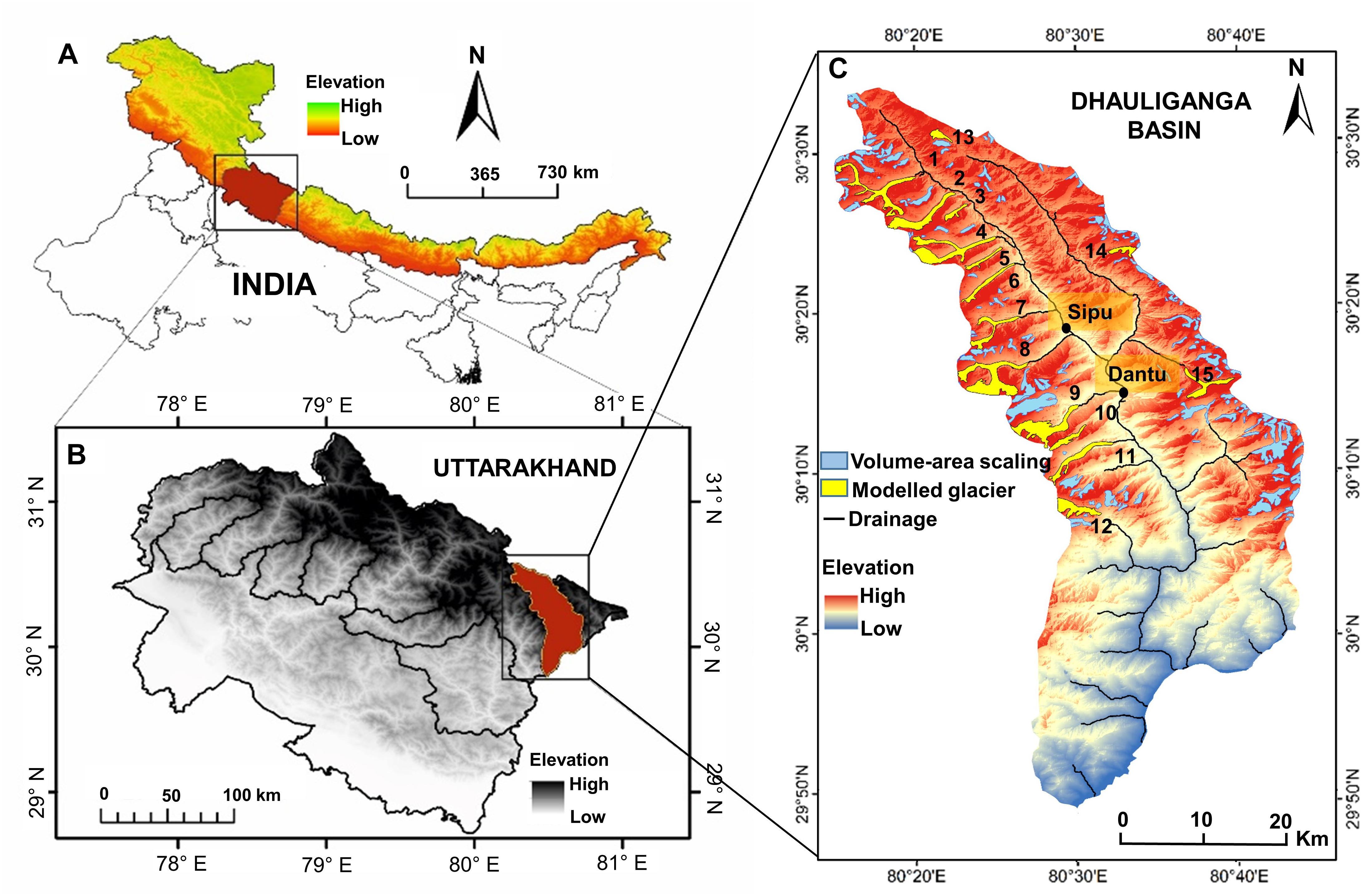
Figure 1. (A) Himalayan arch showing the state of Uttarakhand, Central Himalaya. (B) The location of Dhauliganga Basin, North–east Uttarakhand. (C) Dhauliganga basin showing the glaciers selected for the study.

Data

The present study exploits glacier outlines available in Randolph Glacier Inventory (RGI) which is an open-source database for the existing glaciers in the globe. The latest available version of glacier boundaries (RGI 6.0) is employed for calculating the total volume in the basin (RGI Consortium, 2017). The data can be freely downloaded from http://www.glims.org/RGI. A projection system of UTM-44 was defined to the glacier outlines based on the location of the study region. The Advanced Spaceborne Thermal Emission and Reflection Radiometer (ASTER) global digital elevation model (DEM) (v2) was used to extract topographic information. ASTER GDEM (v2) is a latest version of publicly available elevation model¹ that provides elevation information between 83° N and 83° S with a spatial resolution of 30 m and a vertical accuracy of ∼10–20 m for hilly terrains (Fujita et al., 2008; Tachikawa et al., 2011).

We use Landsat TM and OLI/TIRS (30 m) for glacier mapping in the basin. Two Landsat-8 panchromatic bands (15 m) acquired for consecutive years were used for glacier velocity estimation in the basin, including the validation glaciers. The historical extent of the glaciers was mapped using cloud-free declassified aerial photographs of Corona KH-4 (7.5 m). The Corona database is a collection of very high-resolution aerial images acquired from 1960 to 1972 during a space reconnaissance program, operated jointly by the Central Intelligence Agency (CIA) and the US Air Force (USAF) (Dashora et al., 2007). The Landsat and Corona data used in the study are freely downloaded from https://earthexplorer.usgs.gov/. The acquisition dates and sensor information for the remote sensing datasets are given in Table 1.

TABLE 1

Table 1. Details of the satellite data used.

For the calibration and validation glaciers, available ground measurements of ice thickness were used to compare the model outputs. Ground penetrating radar (GPR) measurements along five transects with a positional accuracy of ±0.1 m and overall uncertainty of ±15 m in ice thickness were used for Chotta Shigri glacier system to calibrate the model inputs (Azam et al., 2012). Similarly, GPR measurements of ice thickness along two transects with a positional accuracy of 1 cm and 7% uncertainty in ice thickness have been used to validate the model for Satopanth glacier system (Mishra et al., 2018). In addition to this, spatially distributed ice thickness of the HF-model by Huss and Farinotti (2012) were employed to compare modeled ice thickness of the calibration and validation glaciers and one glacier in the Dhauliganga basin.

Methodology

In the first phase of the study, satellite imagery has been employed to modify the existing glacier outlines available in RGI (Version 6.0), by mapping the glaciers using a multiple-criteria decision algorithm (Paul et al., 2004). The glaciers chosen for the present study are based on the criteria given in Section “Glacier Selection Criteria.” Furthermore, the investigation incorporates glacier-ice volume estimation of the selected glaciers, using a distributed ice thickness model (see section “Ice Thickness”). The second phase of the study comprises of a multitemporal analysis of satellite imageries to study the glacier fluctuation over the years (see section “Glacier Area Loss”). The description of the methods adopted for the study is given in the following sections.

Glacier Selection Criteria

The 15 larger glaciers (>1 km²) selected for ice thickness modeling, satisfy the following criteria: (i) the obtained velocity field of the glacier is directional with movements from higher to lower elevation, (ii) the glaciers lie entirely within the delineated basin boundary, (iii) the size of the glacier is large enough to map the total area lost using 15 m pan corrected Landsat composite image. Most of the glaciers in the basin fulfill these criteria. The glaciers with an area of less than 1 km² are not considered for thickness modeling due to an inappropriate yield of the velocity field. However, the remaining 159 glaciers with a total area of 82.8 km², have been considered to obtain the total glacier volume in the Dhauliganga basin using a volume-area scaling approach.

Mapping

The remote sensing datasets selected for mapping of the 15 larger (>1 km²) glacier outlines fulfill the following criteria: (i) acquired at the end of ablation season ensuring minimum snow cover, (ii) the presence of minimum cloud coverage in the satellite scene, and (iii) identifiable glacier terminus in both Landsat and Corona satellite imageries. Glacier outlines mapped using Landsat TM and OLI has been considered to estimate ice volume. A few larger glaciers have not been taken into consideration in the retreat analysis due to the unavailability of cloud-free Corona data to map past glacier extent. Unsupervised classification to map glacier boundaries may lead to high level of uncertainties, as most of the glaciers are debris covered in the Himalaya (Kumar et al., 2017). Normalized difference snow index (NDSI) and band ratio method alone is inefficient to map debris-covered glaciers (Bhambri et al., 2011). Hence, the multiple-criteria decision analysis (MCDA) for mapping debris-covered glaciers by thresholding values of TM 4/TM 5, hue, and slope have been exploited (Paul et al., 2004). A band ratio of band 4 (TM 4) and band 5 (TM 5) is computed and a threshold value of 2.0 is applied to distinguish the glacier from its surrounding. Paul (2000) fully justified the accuracy of TM 4/TM 5 band ratio method for glacier mapping by comparing it with the outlines derived using high-resolution SPOT (Satellites Pour l’Observation de la Terre) imageries and thereby establishing an error of less than 1%. The vegetation is distinguished by thresholding the hue component to a value of 126 of an intensity hue-saturation color model developed from TM bands of red, near infra-red (NIR), and short wave infra-red (SWIR). Calculation of glacier slope has been achieved using ASTER GDEM (Abrams et al., 2015). As parts of the glaciers are debris covered a threshold value of <24° is applied to delineate glacier surfaces using slope (Paul et al., 2004). Lastly, an overlay operation of the thematic layers satisfying all the above-mentioned threshold criteria is used to classify glacier surfaces and to map glacier outline (Paul et al., 2004). The terminus of the glacier has been identified by the presence of indicators like a proglacial lake, glacial stream or minimum surface velocity at the snout.

Another challenging task is to orthorectify Corona KH-4 imagery with the aid of ground control points (GCP). Three Corona strips acquired on September 27th, 1968 covering the study area with minimum snow and cloud cover have been employed to map glacier extent in the past. A two-dimensional curve fitting orthorectification technique has been adopted by selecting GCPs on high-resolution orthorectified base imagery. The spline curve fitting method, when applied to a larger spatial extent, may result in residual geometric distortions. Thus, rubber sheeting method for orthorectification is applied to the extracted subsets of the Corona image for each glacier (Bhambri et al., 2011). A total of 70–100 GCPs have been acquired for each Corona subset from Landsat pan-image and high-resolution geo-referenced CNES/Airbus imagery tiles of google-earth. The GCPs were evenly distributed following a gridded pattern to ensure accurate and even co-registration. However, additional GCPs have been collected in and around the glacier boundary to improve local accuracy. A root mean square error (RMSE) for geometric correction in the range of 11–18 m has been achieved. A manual approach to delineate historic glacier boundaries for the year 1968 is employed using the rectified Corona images.

Glacier-Ice Thickness, Glacier Volume and Overdeepings in the Modeled Glacier Bed

Glacier Velocity Estimation

Glacier-surface velocity is obtained by image-to-image correlation at a sub-pixel level using COSI-CORR (Co-registration of Optically Sensed Images and Correlation), a module in ENVI image-processing software. The technique performs co-registration and correlates optical satellite images to calculate the resultant displacement (Scherler et al., 2008). In the present study, we use two Landsat 8 Pan bands, with a temporal interval of 1 year to derive the surface velocity of the glaciers in the Dhauliganga Basin. This method of velocity estimation yields an accuracy of 1/4 of a pixel (Heid and Kääb, 2012). The approach produces N-S and E-W displacement components that are used to estimate the resultant surface movement. A signal to noise filter is finally applied to avoid the anomalous velocity values.

Inaccurate co-registration of the images most often transfer the error to the image matching process, leading to erroneous velocities. To justify the accuracy of the correlation technique, we investigate the RMSE of the displacement measurements obtained over the stable ground in the Dhauliganga basin. In the present study, ice free ground within the basin is assumed to be stable. A total of 334 measurements well spread over the basin is considered, to reveal the shift over the stable ground. The RMSE for E-W component, N-S component, and the resultant displacement is calculated to be 1.4, 0.9, and 0.8 m, respectively (Table 2). The displacement over the stable ground is negligible when compared to the mean resultant displacement of the glaciers in the basin that is measured to be 28 m.

TABLE 2

Table 2. Root mean square error (RMSE) of displacement components obtained over over 149 point locations on the stable ground (assumed to have zero displacement) over 1 year.

Ice Thickness

The present study aims at calculating the glacier-ice volume using two distinct approaches: velocity-slope based modeling and area-based scaling method. In the first approach, the ice thickness distribution of the selected glaciers is computed by equation 1 (Gantayat et al., 2014).

$$H=\sqrt[4]{\frac{1.5Us}{A{\left(f\rho gsin\alpha \right)}^3}}\left(1\right)$$

Where H is the ice thickness in meters, U_s is the surface velocity (derived using image to image correlation of optical satellite image), α is the slope estimated for every 100 m interval, ρ is the ice density, g is the acceleration due to gravity (9.8 ms^-1), f is the shape factor, which is defined as the ratio between the driving stress and basal stress along a glacier (Haeberli and Hoelzle, 1995) and has a range of 0.6 to 1.0, A is the creep parameter which is assigned a constant value of 3.24 × 10^-24 Pa^-3 s^-1 for temperate glaciers (Cuffey and Paterson, 2010). Owing to the unavailability of ground ice thickness measurements in the Dhauliganga Basin, f is calibrated on Chhota Shigri glacier to constrain the value for shape factor (see section “Calibration and Validation of the Model”). The slope calculation has been performed for each elevation distance of 100 m using ASTER GDEM. The ice thickness calculated using pixel-based velocity measurements for different elevation bands using equation 1. It is further mosaicked and converted to individual pixel-based ice thickness point-values using the raster to point GIS-conversion tool. The ice thickness values extracted along the manually digitized flowlines (Linsbauer et al., 2012; Gantayat et al., 2017) are interpolated to obtain a U-shaped ice thickness distribution over the entire glacier area, assuming zero ice thickness along the boundary. The ice volume is thus determined by summing the pixel-wise product of ice thickness and the area of each pixel.

Several scaling methods based on shallow ice approximation enable calculation of mean ice thickness and glacier volume (Bahr et al., 1997). These methods gained widespread acceptance due to the simplicity in both concept and application. In this study, a volume-area scaling is first calibrated to 15 glaciers for which we could directly infer a thickness map using the approach by Gantayat et al. (2014). An intercomparison has been made with the existing power law given by Bahr et al. (1997). The derived volume-area scaling relation is then validated using the total glacier volume of Chhota Shigri glacier (Western Himalaya) and Satopanth glacier (Central Himalaya). The spatially distributed modeled ice thickness of the glaciers is used to calculate the total volume, validated along cross-sections for which ground measurements are available. The total volume of the remaining glaciers in the basin is calculated using a volume-area scaling relation for which the scaling parameters were tuned.

Uncertainty Analysis

The principal causes of the uncertainty are (1) error in surface velocity, (2) uncertain shape factor, (3) glacier-ice density variation, and (4) slope calculation errors. The combined relative uncertainty in glacier-ice volume estimation is determined by the equation derived by taking the natural logarithm of both sides of equation (1) and differentiating:

$$\frac{dH}{H}=0.25\left[\frac{dUs}{Us}-\frac{dA}{A}-3\frac{df}{f}-3\frac{d\rho }{\rho }-3\frac{d(\sin \alpha )}{(\sin \alpha )}\right]\left(2\right)$$

The image-to-image orthorectification errors lead to uncertainty in surface velocity estimation. This, when combined with the error due to image-to-image georectification gives rise to a cumulative error that lies in the range of 3–9 m. The value of dU_s is the difference between the observed and correlated velocity measurements. Since no observed ground velocity measurements were available for the glaciers in the current basin, a value of 3.5 m per year is considered, that is the difference between the observed (Swaroop et al., 2003) and satellite-based glacier-surface velocity outputs as obtained by Gantayat et al. (2014). As f is assumed to be 0.8, which has a range of 0.6 to 1.0, thus the value of df is considered as ±0.2. The value for creep parameter (A) has been considered as 3.24 × 10^-24 Pa^-3 s^-1 (Gantayat et al., 2014). A uniform ice density (ρ) of 900 kg m^-3 throughout the glacier is considered due to unavailability of actual in situ data. It is assumed the ice density may decrease up to 850 kg m^-3. An uncertainty of 5.5% calculated when dρ is 50 kg m^-3. Also, the unavailability of ground elevation measurement for the study area to estimate the uncertainty in slope calculation bound us to consider 11 m as vertical inaccuracy for ASTER DEM calculated for the Himalayan region (Fujita et al., 2008). The uncertainty due to inherent DEM error is given by d (sin α) and is calculated to be 0.11 m.

Identification of the Overdeepening Sites

The spatial distribution of glacier-ice thickness obtained using raster-based modeling technique can be used to extract information pertaining to glacier bed topography (Linsbauer et al., 2009). The overdeepening sites in the glacier bed are potential lake formation sites, as these depressions may hold water after the withdrawal of the overlying ice in the future (Linsbauer et al., 2012; Frey et al., 2014; Maanya et al., 2016). The bed topography of the individual glacier is determined by subtracting the ice thickness from the surface topography of the respective glaciers using GIS-based tools. The sinks in the glacier bed thus formed, are filled with the aid of arc-hydro tools for discrete identification of the overdeepening sites.

Glacier Area Loss

The overall glacier area loss has been determined by calculating the difference in the spatial extent of the glaciers in 1968 and 2016, derived using Corona and Landsat imagery, respectively. In order to understand the behavior of the individual glaciers based on their size and ice thickness, a statistical analysis has been adopted to determine the dependency of the relative area change of the glaciers to that of the total glacier area in 1968. Also, a similar analysis has been performed by plotting relative area loss versus mean modeled ice thickness near the terminus. Figure 2 shows a loss in glacier area and lake growth of the highest lake in the Dhauliganga basin over a period of 48 years from 1968 and 2016.

FIGURE 2

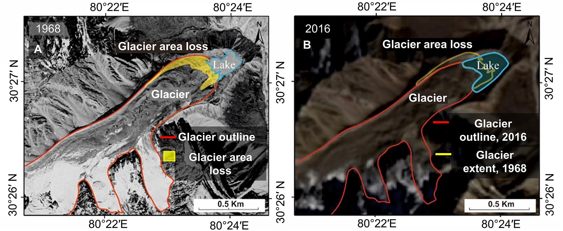
Figure 2. Glacier area loss and change in the lake extent from 1968 to 2016 for glacier IN 5O103 04 030 (^∗GSI ID) shown over base imagery of (A) Corona- KH4 and (B) pan-corrected L8 composite image. (^∗Geological survey of India).

Calibration and Validation of the Model

The distributed ice thickness model adopted in the present study is calibrated on the Chhota Shigri glacier (Western Himalaya) and validated on the Satopanth glacier system (Central Himalaya). Ice thickness distribution was calculated for each glacier as in Section “Ice Thickness.” Glacier-surface velocity was calculated using the same approach as Section “Glacier Velocity Estimation.”

For Chhota Shigri glacier, surface velocity is calculated for 2000–2001 and 2016–2017, revealing mean velocities of 20 and 21 m yr^-1, respectively. A near-zero displacement is evident over the ice free stable ground. The velocity vectors show a directional flow with surface velocities up to 25–28 m yr^-1 at the central part of the glacier. Figures 3A,B shows the velocity-vector field calculated based on the correlation of remotely sensed images. The satellite-derived velocity measurements were validated using the available ground velocities given by Azam et al. (2012) (Figure 3C). The accuracy of the satellite-derived velocity was evaluated by direct comparison with the field-based velocity measurements obtained for the year 2000–2001 and 2016–2017 resulting in an RMSE of 2.2 and 2.5 m yr^-1, respectively. Also, glacier velocity (2000–2001) versus glacier velocity (2016–2017) shows a high correlation with a linear correlation coefficient of 0.91 (Figure 3D). Thus, it can be assumed that the glacier-surface velocity does not change much over the given period of time and therefore the output velocities are assumed to be suitable for thickness reconstruction, despite their temporal separation. Ice thickness calculation was performed for two different shape factors (f) (0.6 and 0.8) to better constrain the value of f. The modeled ice thickness was validated using GPR bed profiles (Azam et al., 2012) along five cross-sections. The RMSE is calculated by taking the difference in the ice thickness at 10 uniformly distributed points along each cross-section. The value f = 0.8 yielded ice thickness, highly comparable to the ground measurements with an RMSE of 12–23% and therefore seems reasonable to assume the applicability of the present approach and the given model parameters to other Himalayan glaciers. Moreover, the modeled glacier-bed profiles show a mean difference of ∼15% when compared to the ones obtained using Huss and Farinotti (2012). Figure 4 shows the modeled ice thickness distribution plot and a comparison of the glacier bed profiles along the cross-sections.

FIGURE 3

Figure 3. Satellite-derived velocity field of Chhota Shigri glacier for (A) 2000–2001 and (B) 2016–2017; displacement over stable ground is nearly zero; discarded vectors are based on signal to noise filtering. (C) Satellite-derived velocity (2000–2001 and 2016–2017) and field-based velocity (2003–2004) (Azam et al., 2012) at different elevations. (D) Glacier velocity (2000–2001) versus glacier velocity (2016–2017).

FIGURE 4

Figure 4. (A–E) Comparision of the model-derived glacier bed profiles of Chhota Shigri glacier (f = 0.6 and f = 0.8) with the GPR measurements by Azam et al. (2012) and Huss and Farinotti (2012). (F) Ice thickness distribution of Chhota Shigri glacier (Western Himalaya) showing transects of the glacier bed profiles; the outlines of the overdeepening sites have been marked by red (Present Study) and yellow (Huss and Farinotti, 2012).

The Satopanth glacier system, over which we perform a validation assessment is located in the adjacent basin (Alaknanda) of the present study area in Central Himalaya. The glacier-ice thickness distribution is calculated using the same set of model inputs as that in the calibration setup. Since f was calibrated on the Chotta Shigri glacier to a value of 0.8, we validate the model by directly comparing the modeled ice thickness (f = 0.8) of Satopanth glacier to the GPR measurements available along two transects, one near the terminus and the other at 10 km upstream of the snout (Mishra et al., 2018). Figure 5 shows the glacier-surface velocity field, modeled ice thickness distribution and the modeled glacier-bed profiles (f = 0.6 and f = 0.8). The modeled glacier-bed profile is plotted against the GPR measurements along a transverse transect near the terminus (Figure 5C) and also compared at a point location along a GPR transect in the upper part of the glacier (Figure 5D). The RMSE when f = 0.8 is calculated to be 8.03 m. The results obtained using Huss and Farinotti (2012) is compared to the modeled ice thickness (f = 0.8) along each transect (Figures 5C,D), resulting in an RMSE of 12.1 m.

FIGURE 5

Figure 5. (A) Satellite-derived velocity vectors of Satopanth glacier (Western Himalaya). (B) Distributed ice thickness of the Satopanth glacier. (C,D) Comparison of the model-derived glacier bed profiles (f = 0.6 and f = 0.8) with the GPR measurements by Huss and Farinotti (2012) and Mishra et al. (2018).

Results

In the present study, glacier volume was calculated for 15 larger (>1 km²) glaciers in the Dhauliganga Basin, Central Himalaya. The study applies a glacier-surface velocity based method to model the ice thickness distribution for the given glaciers. The method was first applied to Chotta Shigri and the Satopanth glacier for model calibration and validation, respectively. In addition, the total volume of the basin is calculated using a volume-area scaling power law in the form of V = c × S^γ for which the scaling parameters were tuned based on regression of the modeled volumes.

Since field measurements of glacier-surface velocity are very sparse and involve rigorous fieldwork, a remote sensing based method to estimate glacier velocity was employed in the study. The satellite-based velocity measurements yielded a mean velocity of 27 m yr^-1 for all the glaciers selected for the study. The maximum velocity of the glaciers occurs in the range of 50–70 m yr^-1. The glaciers exhibit highly directional flow with higher velocities in the upper part of the ablation zone, gradually decreasing toward the terminus of the glaciers. The glacier-surface velocity and the modeled ice thickness distribution of the glacier GSI ID-IN 5O103 04 015 are shown in Figures 6A,C, respectively. The observed mean velocity of the illustrated glacier is estimated to be 23 m yr^-1 with a mean thickness of 63 m and total ice volume of 7.2 × 10⁸ m³. The empirically derived ice thickness distribution of the glacier is compared to estimates calculated using Huss and Farinotti (2012) (Figure 6B). The cross-sectional glacier bed profiles are plotted along four transects aa′, bb′, cc′, and dd′ as shown in Figure 6D. The comparative analysis of the cross-sections yields an average RMSE of 21 m for all cross-sections.

FIGURE 6

Figure 6. (A) Satellite-derived glacier-surface velocity of Glacier 8 (GSI ID-IN 5O103 04 015). (B) Ice thickness distribution of Glacier 8 (Huss and Farinotti, 2012). (C) Empirically derived ice thickness distribution for Glacier 8 (Present Study). The central part of the main trunk has a maximum ice thickness of 230 m. Near the terminus, the thickness is estimated to be approximately 20 m. The overdeepening sites are marked in gray; subset shows the longitudinal glacier-bed profile along ee′. (D) Comparison of the modeled cross-sectional glacier bed profiles with Huss and Farinotti (2012), along four cross-sectional profiles given as aa′, bb′, cc′, and dd′.

The sparingly available ground ice thickness measurements for validation is a major limitation of the approach when applied over the Himalaya. A calibration and validation assessment on the Chotta Shigri and Satopanth glacier system (see section “Methodology”), has shown good agreement between GPR measurements and modeled ice thickness. The calibration of the model constrained the value of the valley shape factor (f) to 0.8. For Satopanth glacier, an overestimation of the total modeled glacier volume by 14.7% using the present approach was evident when f = 0.6. The total modeled volume (f = 0.8) of the 15 selected larger (>1 km²) glaciers in Dhauliganga basin is estimated to be 3.78 × 10⁹ m³ which is equivalent to 3.3 ± 0.5 Gt of ice mass. A total uncertainty is modeled volume is estimated to be 18.4% (see section “Uncertainty Analysis”). The details of the glacier area, ice thickness, and volume are enlisted in Table 3.

TABLE 3

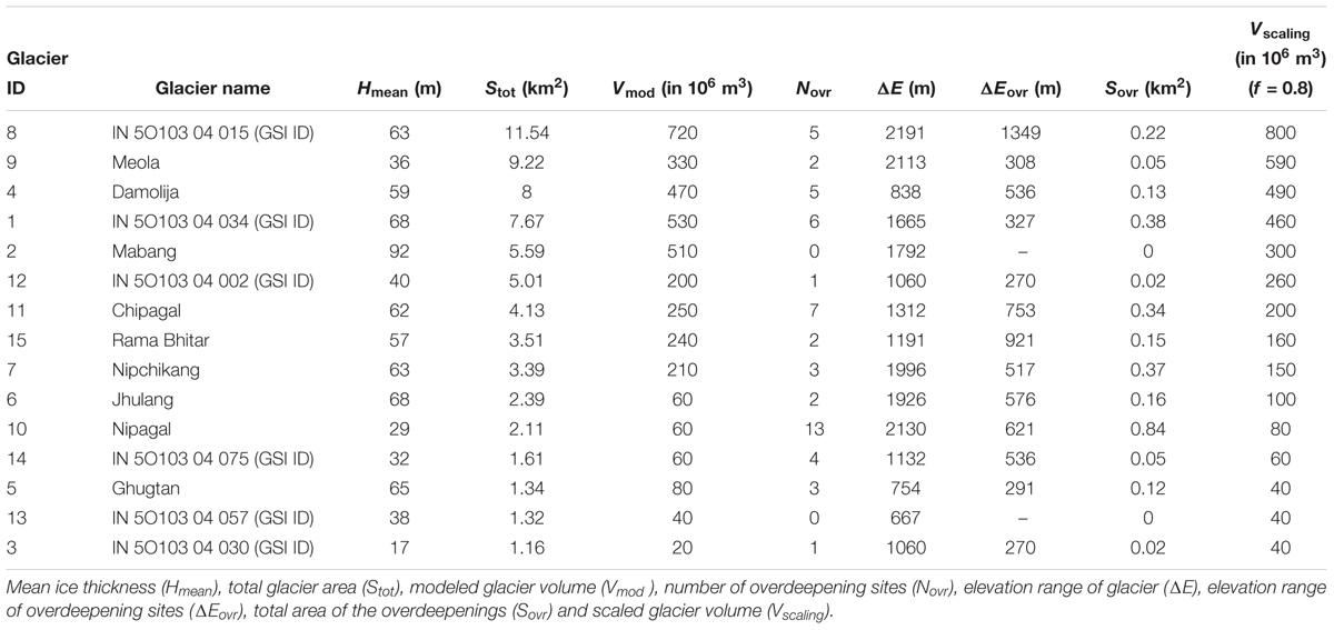
Table 3. Glacier volume derived from the calibrated volume-area scaling relation.

The empirically derived glacier volume versus area regression analysis has been performed for the 15 individual glaciers in the basin. Two sets of modeled volume calculated using different shape factor (f = 0.6 and f = 0.8) are plotted against the respective total glacier area. In both cases, a linear trend is clearly evident. However, the analysis yielded two different volume-area scaling power-law relationships. The level of agreement between the data points for f = 0.6 and f = 0.8 yielded a coefficient of determination of 0.87 and 0.92, respectively. The power law relation obtained for f = 0.6 can be stated as V = 0.030 × S^1.31 and that of f = 0.8 is V = 0.029 × S^1.34 where ‘V’ is the total volume and ‘S’ is the total area of the glacier. Figure 7 shows the volume-area regression plots of the selected glaciers, for which volume is calculated for different values of f (0.6 and 0.8) and also using the volume-area scaling given by Bahr et al. (1997). The obtained scaling (f = 0.8) relation is applied to Chhota Shigri glacier (Western Himalaya) and Satopanth glacier (Central Himalaya), for which modeled ice thickness was validated using the available ground truth. The derived volume-area scaling thereby yielded a total volume with an accuracy of 95.6 and 95.1% for Chhota Shigri and Satopanth glacier, respectively, when compared to their modeled volume. Further tuning of the scaling parameters on the Chhota Shigri and the Satopanth system for better accuracy, yielded a relation which is given by V = 0.030 × S^1.34. The total modeled volume (f = 0.8) of the selected glaciers has a difference of less than 1% when compared to the calculated volume using the proposed volume-area scaling (V = 0.030 × S^1.34). The overestimation of the modeled glacier volume (f = 0.8) of the selected glaciers by 1.4 × 10⁸ m³ (3.8%) using Bahr et al. (1997) suggested the scope of minor tuning in the scaling coefficients of the volume area scaling relation. As area-based scaling method is region specific, the revision of the scaling parameters in the present study yields a more realistic area-volume relation for the given geographical region.

FIGURE 7

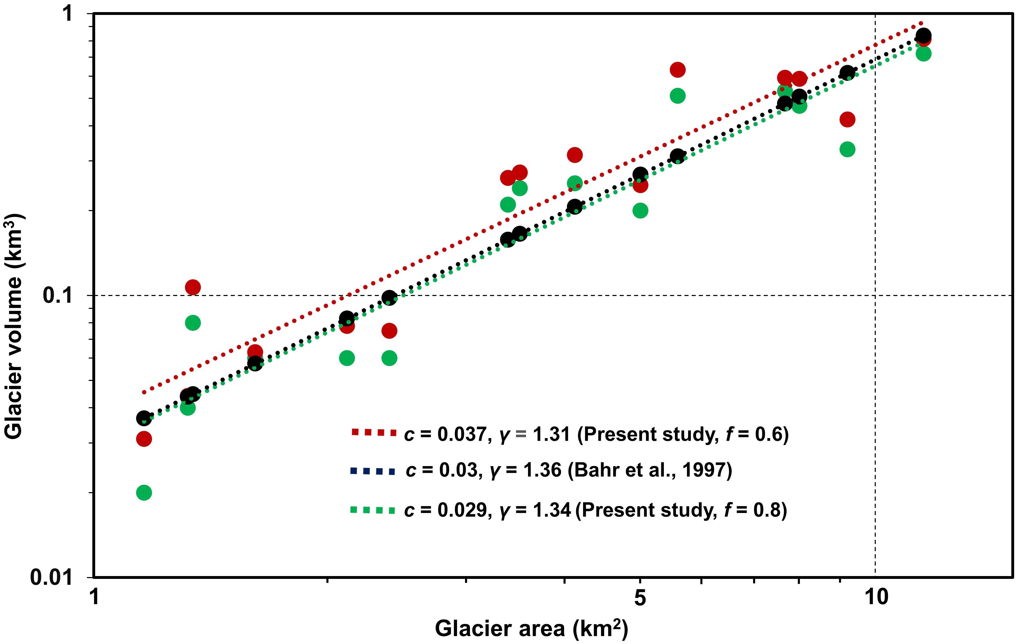
Figure 7. Glacier volume (km³) versus glacier area (km²) for different values of f; the volume-area scaling relations derived from these results in the form of V = c × S^γ are V = 0.037 × S^1.31 (f = 0.6), V = 0.029 × S^1.34 (f = 0.8), and V = 0.030 × S^1.36 (Bahr et al., 1997).

The ice volume for the remaining glaciers excluding the 15 larger glaciers was calculated using the above derived volume-area scaling is 2.71 × 10⁹ m³. The total calculated glacier-ice volume of the basin is calculated to be 6.5 × 10⁹ m³. The total ice volume of the selected glaciers estimated using the present approach is ∼8% higher than the estimates calculated using the approach by Huss and Farinotti (2012). Also, the total volume calculated relation by Bahr et al. (1997) overestimates it by 1.6 × 10⁸ m³.

In addition, evaluation of the glacier bed led to the discrete identification of topographic depressions on the glacier bed. The presence of these depressions at the frontal part of the glacier may lead to formations of proglacial lakes in the near future, as compared to those sites identified in the higher elevation ranges of the glaciers. A total of 54 overdeepening sites with a total area of 2.93 km² were identified, as enumerated in Table 3. The highest number of overdeepening sites are identified in the bed of Nipagal glacier covering an area of 0.84 km². The total overdeepening sites identified in the basin has a volume capacity to hold 15.1 × 10⁷ m³ of water.

Furthermore, the analysis using multi-temporal satellite imagery showed a total of approximately 4.65 km² loss in the total glacier area for the selected glaciers over a span of 48 years from 1969 to 2016. The mean rate of loss is thus calculated to be 0.09 km² yr^-1. To understand the behavior of the individual glacier based on its size and ice thickness, a statistical analysis has been adopted to determine the dependency of the relative area change of the selected glaciers to that of the total glacier area in 1968. It is evident that, of the 15 glaciers selected for the study, smaller glaciers show higher relative change as compared to the larger ones. The smallest glacier reacts very individually. The study is in line with similar findings by Paul (2002) where the dependency of relative area change shows a similar trend, in which the smallest glaciers reacting individually and the larger glaciers show a similar relative change in glacier area. The dependency of relative area change to the modeled mean ice thickness near terminus reveals a similar trend as that of relative area change versus area in 1968. This may be attributed to the fact that larger glaciers have greater ice thickness near the terminus as compared to the smaller glacier (Kulkarni et al., 2011). Figure 8 shows the plot of the relative change (%) in the glacier area between 1968 and 2016 versus glacier area in 1968 and mean ice thickness near the terminus. Also, the growth of the highest pro-glacial lake due to the retreat of the associated glacier in the Dhauliganga basin (Figure 2) is a potential threat to the downstream regions. The formation of such lakes invariably hastens glacier mass loss as they are in direct contact with the glacier (Linsbauer et al., 2012).

FIGURE 8

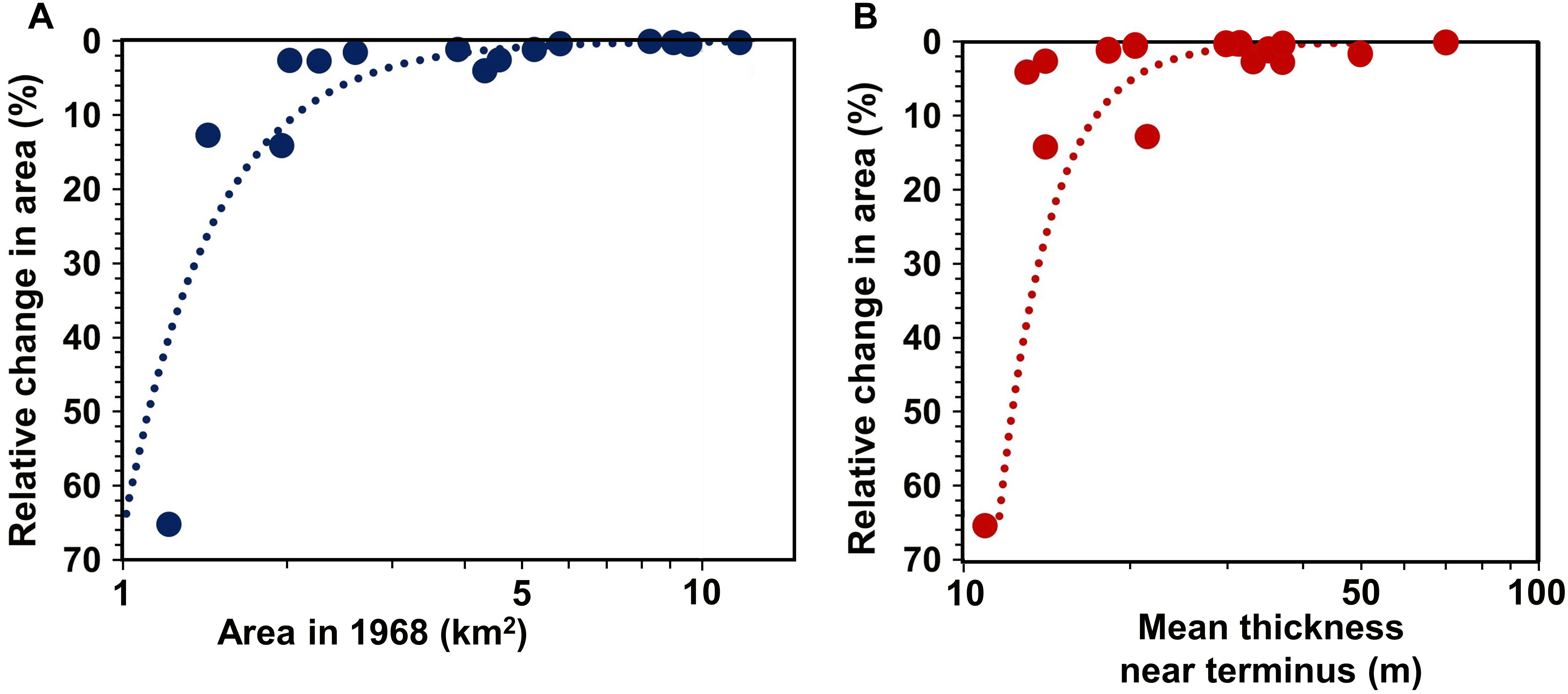
Figure 8. Relative area changes between 1968 and 2016 versus (A) glacier area in 1968 and (B) mean ice thickness near the terminus.

Discussion

Model Sensitivity

The sensitivity of the ice thickness to surface velocity (U_s), valley shape factor (f), and creep-factor (A) and ice density (ρ) was computed for Chhota Shigri glacier. Results indicated that the total glacier volume changes by 1.4 × 10⁸ m³ (10.1%) and 2.5 × 10⁸ m³ (17.8%) with an increment or decrement of the shape factor by 0.1 and 0.2, respectively. This sensitivity can be traced in the glacier thickness profiles along the central-line for different f-values as shown in Figure 9B. A shape factor (f) of 0.6 yielded glacier-ice thickness with a maximum thickness. An increase in f by 0.1 and 0.2 resulted in the maximum thickness by 10.8 and 19.2%, respectively. The sensitivity of ice thickness to creep parameter (A) is shown in Figure 9D. The glacier volume changes by 4.0 × 10⁷ m³ (2.8%) when the creep factor is changed from 3.24 × 10^-24 Pa^-3 s^-1 (Gantayat et al., 2014) to 2.4 × 10^-24 Pa^-3 s^-1 (Farinotti et al., 2009a). In addition, the sensitivity of the model to surface velocity is tested by increasing the remotely derived velocity by 10 and 20% yielding ice volume higher by 3.6 and 7.4%, respectively. Figure 9A shows the ice thickness for different surface velocities. The sensitivity of ice thickness to ice density change was performed by taking into consideration different ice densities (ρ) of 850 and 900 kg m^-3. The resultant glacier-ice volume had a difference of 3.0 × 10⁷ m³ (2.2%). The glacier-ice thickness for the different ρ values is shown in Figure 9C. The method of selecting branch lines also affect the ice thickness measurements. In case of a single branch line, a V-shaped glacier bed profile is obtained. The present study follows the rules by Paul and Linsbauer (2012) to obtain a U-shaped bed profile. The ice thickness model results are least sensitive to changes in the basal velocity (U_b) (Gantayat et al., 2014) and which has been neglected in the present study. The linear error propagation of the distributed ice thickness model assuming certain input uncertainties in the various input parameters is given in Section “Uncertainty Analysis.”

FIGURE 9

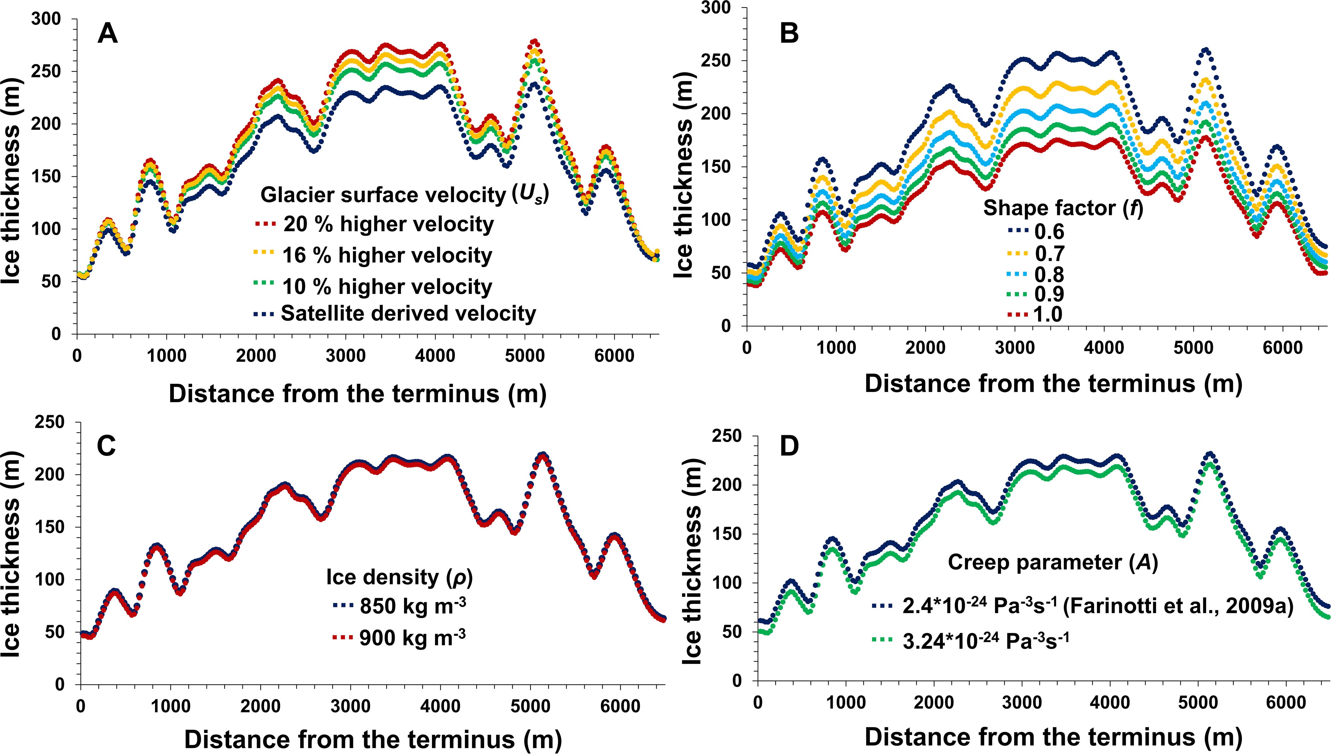
Figure 9. Sensitivity of modeled ice thickness to (A) surface velocity U_s, (B) the shape factor f, (C) the ice density ρ, and (D) the creep parameter A.

The analysis shows that the ice thickness model adopted in the present study is most sensitive to changes in valley shape factor (f) as compared to the other input parameters. Therefore, it is suggested to calibrate the model to better constrain the value of f, wherever direct measurements on ice thickness are available. The model sensitivity versus uncertainty is analyzed to confirm the overall calculated uncertainty in the ice thickness distribution. The total ice volume calculated in the sensitivity analysis varied by 17.6%, considering the same parameter ranges as given in Section “Uncertainty Analysis.”

Volume-Area Scaling- Uncertainty and Sensitivity

The uncertainty and the sensitivity of the volume-area scaling proposed in the present study are described in this section. For this, we have divided the 15 glaciers selected for the study into 75 different parts (subsets) based on random area. The scaling relationship is tested using regression of empirically derived glacier volume for 75 random parts, by plotting their respective area versus its modeled volume calculated for each part. This regression analysis yields a power law which is given as V = 0.037 × S^1.34. The scaling parameters obtained are compared to the tuned volume area relation. The exponent γ in V = c × S^γ remains unchanged and a difference of 23% in the value of c is calculated when compared to the tuned volume-area scaling (V = 0.030 × S^1.34). Figure 10 shows the plot of modeled volume versus area for the 75 glacier subsets and also volume versus area using the tuned volume-area scaling.

FIGURE 10

Figure 10. Modeled volume (km³) versus area (km²) of respective random glacier subsets (Blue) and tuned area-based scaled volume (km³) versus glacier area (km²) for the given subsets (V = 0.030 × S^1.34) (Red).

The sensitivity of the derived volume-area scaling is evaluated by varying the model parameters and computing ice volume for the 15 glaciers. The scaling parameters were recomputed for all the glaciers to see the effect on the total glacier volume. The sensitivity of the volume-area scaling to valley shape factor (f), and creep-factor (A), and ice density (ρ) was computed (Figure 11). Results indicate that the total glacier volume increase or decrease by 4.1 × 10⁸ m³ (11%) and 7. 5 × 10⁸ m³ (20%) when f is varied by 0.1 and 0.2, respectively. Similarly, total volume changes by 2.4 × 10⁸ m³ (6.4%) when A is changed from 2.4 × 10^-24 Pa^-3 s^-1 (Farinotti et al., 2009a) to 3.24 × 10^-24 Pa^-3 s^-1 (Gantayat et al., 2014). The sensitivity of the volume-area scaling is tested for ice density (ρ) by changing the density by 50 kg m^-3. The total volume of the glaciers changes by 3.1% after density variation is applied. The volume-area scaling is most sensitive to the shape factor (f) as compared to the other model input parameters. From the sensitivity analysis it is conclusive that both, the distributed ice thickness model and the derived volume-area scaling are most sensitive to changes in f.

FIGURE 11

Figure 11. Glacier volume (km³) versus glacier area (km²) using different values of (A) the shape factor f, (B) the creep parameter A, and (C) glacier-density ρ; total number of glaciers is given by n.

Conclusion

The current study is an assessment of the two most vital aspects of the Himalayan cryosphere- glacier-ice volume and glacier-area loss. Previous efforts to estimate glacier volume using velocity-based modeling technique mainly focused on a single glacier. In this comprehensive study, the total glacier-ice volume has been estimated for an entire central Himalayan basin. The study also provides insight into the temporal fluctuations of glacier extent over a period of 48 years. The future shrinkage of the glacier area needs a more detailed investigation to understand its intrinsic relationship with its surrounding climate. Moreover, sustainability assessment of the glaciers by knowing the total glacier volume at present would help in the strategic management of the stored freshwater reserves in the Himalaya.

The raster-based modeling technique enabled determination of spatially distributed glacier-ice thickness and expansion of the study over a broader geographical area. We characterized 15 larger glaciers in the basin in terms of its distributed ice thickness. The mean ice thickness of the glaciers range from 17 to 92 m. The comparison of the modeled ice thickness and GPR measurements of two Himalayan glaciers shows that the method is well suited to estimate total glacier volume in the region. The total modeled volume of the 15 larger glaciers is computed to be 3.78 × 10⁹ m³ (f = 0.8) with an uncertainty of 18.4%. Huss and Farinotti (2012) presented a distributed ice thickness and volume of all the glaciers in the world. An inter-comparative evaluation of our model-derived glacier ice thickness to that of Huss and Farinotti (2012) was performed.

The area-based scaling approach (Bahr et al., 1997) resulted in an overestimation of total glacier volume by 1.4 × 10⁸ m³ for the selected larger glaciers. This led to the scope of minor tuning in the scaling coefficients. In the calibration of the volume-area scaling relation (V = c × S^γ) c remains unchanged and γ changes from 1.36 to 1.34, when compared to Bahr et al. (1997). Thus, a volume-area scaling power law (V = 0.030 × S^1.34) is derived for the given Himalayan basin by tuning the scaling parameters. The volume of the remaining glaciers apart from the 15 larger glaciers in the basin calculated using volume area scaling is 2.71 × 10⁹ m³. The total volume of the basin is computed to be 6.5 × 10⁹ m³. The ice thickness model was employed to discretely map the glacier bed and identify the overdeepening sites. A total of 54 overdeepening sites were identified in the basin with a volume capacity to hold 15.1 × 10⁷ m³ of water. The identification of these sites on the glacier bed is crucial, as these depressions identified over the glacier bed may form high altitude lakes in the future (Linsbauer et al., 2012).

Author Contributions

AS gathered and prepared all data, performed all calculations, and made all figures. AS, AG, and AK contributed to the discussion of results and shared in writing the manuscript. AS and PD contributed to carrying out GIS analysis.

Funding

AS received financial support from the Government of India, DST INSPIRE Fellowship programme to carry the research work.

Conflict of Interest Statement

The authors declare that the research was conducted in the absence of any commercial or financial relationships that could be construed as a potential conflict of interest.

Acknowledgments

We acknowledge the IIT Roorkee, for providing necessary laboratory and infrastructure facilities. We thank Dr. Matthias Huss, ETH Zurich for providing valuable data for validation. We are grateful to RGI consortium, USGS for its free data policy, allowing us to use the glacier outlines, Landsat TM/ETM+, Corona KH4, and ASTER GDEM. AS acknowledges the Government of India, DST INSPIRE Fellowship for the financial support to carry the research work.

Footnotes

1. ^ https://earthexplorer.usgs.gov/

References

Abrams, M., Tsu, H., Hulley, G., Iwao, K., Pieri, D., Cudahy, T., et al. (2015). The advanced spaceborne thermal emission and reflection radiometer (ASTER) after fifteen years: review of global products. Int. J. Appl. Earth Obs. Geoinf. 38, 292–301. doi: 10.1016/j.jag.2015.01.013

CrossRef Full Text | Google Scholar

Armstrong, R. L. (2010). The Glaciers of the Hindu Kush-Himalayan Region: A Summary of the Science Regarding Glacier Melt/Retreat in the Himalayan, Hindu Kush, Karakoram, Pamir, and Tien Shan Mountain Ranges. Kathmandu: International Centre for Integrated Mountain Development (ICIMOD).

Google Scholar

Azam, M. F., Wagnon, P., Ramanathan, A., Vincent, C., Sharma, P., Arnaud, Y., et al. (2012). From balance to imbalance: a shift in the dynamic behaviour of Chhota Shigri glacier, western Himalaya, India. J. Glaciol. 58, 315–324. doi: 10.3189/2012JoG11J123

CrossRef Full Text | Google Scholar

Bahr, B., Meier, F., and Peckham, S. D. (1997). The physical basis of glacier volume-area scaling perturbations in the ice mass balance rate D (rate of ice accumulation area at relatively high elevations low elevations (D < 0 on a yearly average), Volume-Size. J. Geophys. Res. 102, 355–362. doi: 10.1029/97JB01696

CrossRef Full Text | Google Scholar

Bennett, G. L., and Evans, D. J. A. (2012). Glacier retreat and landform production on an overdeepened glacier foreland: the debris-charged glacial landsystem at Kvíárjökull, Iceland. Earth Surf. Process. Landforms 37, 1584–1602. doi: 10.1002/esp.3259

CrossRef Full Text | Google Scholar

Bhambri, R., and Bolch, T. (2009). Glacier mapping: a review with special reference to the Indian Himalayas. Prog. Phys. Geogr. 33, 672–704. doi: 10.1177/0309133309348112

CrossRef Full Text | Google Scholar

Bhambri, R., Bolch, T., Chaujar, R. K., and Kulshreshtha, S. C. (2011). Glacier changes in the Garhwal Himalaya, India, from 1968 to 2006 based on remote sensing. J. Glaciol. 57, 543–556. doi: 10.3189/002214311796905604

CrossRef Full Text | Google Scholar

Bolch, T., Kulkarni, A., Kääb, A., Huggel, C., Paul, F., Cogley, J. G., et al. (2012). The state and fate of himalayan glaciers. Science 336, 310–314. doi: 10.1126/science.1215828

PubMed Abstract | CrossRef Full Text | Google Scholar

Brinkerhoff, D. J., Aschwanden, A., and Truffer, M. (2016). Bayesian inference of subglacial topography using mass conservation. Front. Earth Sci. 4:8. doi: 10.3389/feart.2016.00008

CrossRef Full Text | Google Scholar

Chen, J., and Ohmura, A. (1990). “Estimation of alpine glacier water resources and their change since the 1870s,” in I—Hydrology in Mountainous Regions: Hydrologic Measurements, the Water Cycle. Hydrology in Mountainous Regions I, (Oslo: International Association of Hydrological Sciences Publication 193), 127–135.

Google Scholar

Clarke, G. K. C., Anslow, F. S., Jarosch, A. H., Radiæ, V., Menounos, B., Bolch, T., et al. (2013). Ice volume and subglacial topography for western Canadian glaciers from mass balance fields, thinning rates, and a bed stress model. J. Clim. 26, 4282–4303. doi: 10.1175/JCLI-D-12-00513.1

CrossRef Full Text | Google Scholar

Cuffey, K. M., and Paterson, W. S. B. (2010). The Physics of Glaciers. Cambridge, MA: Academic Press.

Google Scholar

Dashora, A., Lohani, B., and Malik, J. N. (2007). A repository of earth resource information - CORONA satellite programme. Curr. Sci. 92, 926–932. doi: 10.2307/24097673

CrossRef Full Text | Google Scholar

Dyurgerov, M. B., and Meier, M. F. (1997). Year-to-year fluctuations of global mass balance of small glaciers and their contribution to sea-level changes. Source Arct. Alp. Res. Arct. Alp. Res. 29, 392–402. doi: 10.2307/1551987

CrossRef Full Text | Google Scholar

Dyurgerov, M. B., and Meier, M. F. (2005). Glaciers amd the Changing Earth System: A 2004 Snapshot. Boulder: INSTAAR.

Google Scholar

Farinotti, D., Brinkerhoff, D. J., Clarke, G. K. C., Fürst, J. J., Frey, H., Gantayat, P., et al. (2017). How accurate are estimates of glacier ice thickness? Results from ITMIX, the Ice Thickness Models Intercomparison eXperiment. Cryosphere 11, 949–970. doi: 10.5194/tc-11-949-2017

CrossRef Full Text | Google Scholar

Farinotti, D., Huss, M., Bauder, A., Funk, M., and Truffer, M. (2009a). A method to estimate the ice volume and ice-thickness distribution of alpine glaciers. J. Glaciol. 55, 422–430. doi: 10.3189/002214309788816759

CrossRef Full Text | Google Scholar

Farinotti, D., Huss, M., Bauder, A., and Funk, M. (2009b). An estimate of the glacier ice volume in the Swiss Alps. Glob. Planet. Chang. 68, 225–231. doi: 10.1016/j.gloplacha.2009.05.004

CrossRef Full Text | Google Scholar

Farinotti, D., Huss, M., Fürst, J. J., Landmann, J., Machguth, H., Maussion, F., et al. (2019). A consensus estimate for the ice thickness distribution of all glaciers on Earth. Nat. Geosci. 12, 168–173. doi: 10.1038/s41561-019-0300-3

CrossRef Full Text | Google Scholar

Frey, H., Machguth, H., Huss, M., Huggel, C., Bajracharya, S., Bolch, T., et al. (2014). Estimating the volume of glaciers in the Himalayan–Karakoram region using different methods. Cryosphere 8, 2313–2333. doi: 10.5194/tc-8-2313-2014

PubMed Abstract | CrossRef Full Text | Google Scholar

Fujita, K., Suzuki, R., Nuimura, T., and Sakai, A. (2008). Performance of ASTER and SRTM DEMs, and their potential for assessing glacial lakes in the Lunana region, Bhutan Himalaya. J. Glaciol. 54, 220–228. doi: 10.3189/002214308784886162

CrossRef Full Text | Google Scholar

Gantayat, P., Kulkarni, A. V., and Srinivasan, J. (2014). Estimation of ice thickness using surface velocities and slope: case study at Gangotri Glacier, India. J. Glaciol. 60, 277–282. doi: 10.3189/2014JoG13J078

CrossRef Full Text | Google Scholar

Gantayat, P., Kulkarni, A. V., Srinivasan, J., and Schmeits, M. J. (2017). Numerical modelling of past retreat and future evolution of Chhota Shigri glacier in Western Indian Himalaya. Ann. Glaciol. 58, 136–144. doi: 10.1017/aog.2017.21

CrossRef Full Text | Google Scholar

Haeberli, W., and Hoelzle, M. (1995). Application of inventory data for estimating characteristics of and regional climate-change effects on mountain glaciers: a pilot study with the European Alps. Ann. Glaciol. 21, 206–212. doi: 10.3189/S0260305500015834

CrossRef Full Text | Google Scholar

Heid, T., and Kääb, A. (2012). Evaluation of existing image matching methods for deriving glacier surface displacements globally from optical satellite imagery. Remote Sens. Environ. 118, 339–355. doi: 10.1016/j.rse.2011.11.024

CrossRef Full Text | Google Scholar

Huss, M., and Farinotti, D. (2012). Distributed ice thickness and volume of all glaciers around the globe. J. Geophys. Res. Earth Surf. 117, 1–10. doi: 10.1029/2012JF002523

CrossRef Full Text | Google Scholar

Huss, M., Farinotti, D., Bauder, A., and Funk, M. (2008). Modelling runoff from highly glacierized alpine drainage basins in a changing climate. Hydro. Proc. 22, 3888–3902. doi: 10.1002/hyp.7055

CrossRef Full Text | Google Scholar

Johannesson, T., Raymond, C. F., and Waddington, E. D. (1989). Time- scale for adjustment of glaciers to changes in mass balance. J. Glaciol. 35, 355–369.

Google Scholar

Kaser, G., Grosshauser, M., and Marzeion, B. (2010). Contribution potential of glaciers to water availability in different climate regimes. Proc. Natl. Acad. Sci. U.S.A. 107, 20223–20227. doi: 10.1073/pnas.1008162107

PubMed Abstract | CrossRef Full Text | Google Scholar

Kulkarni, A. V., Bahuguna, I. M., Rathore, B. P., Singh, S. K., Randhawa, S. S., Sood, R. K., et al. (2007). Glacial retreat in Himalaya using Indian remote sensing satellite data. Curr. Sci. 92, 69–74. doi: 10.1117/12.694004

CrossRef Full Text | Google Scholar

Kulkarni, A. V., Dhar, S., Rathore, B. P., Babu Govindha Raj, K., and Kalia, R. (2006). Recession of samudra tapu glacier, Chandra river basin, Himachal Pradesh. J. Indian Soc. Remote Sens. 34, 39–46. doi: 10.1007/BF02990745

CrossRef Full Text | Google Scholar

Kulkarni, A. V., and Karyakarte, Y. (2014). Observed changes in Himalayan glaciers. Curr. Sci. 106, 237–244.

Google Scholar

Kulkarni, A. V., Rathore, B. P., Singh, S. K., and Bahuguna, I. M. (2011). Understanding changes in the Himalayan cryosphere using remote sensing techniques. Int. J. Remote Sens. 32, 601–615. doi: 10.1080/01431161.2010.517802

CrossRef Full Text | Google Scholar

Kumar, V., Mehta, M., Mishra, A., and Trivedi, A. (2017). Temporal fluctuations and frontal area change of Bangni and Dunagiri glaciers from 1962 to 2013, Dhauliganga Basin, central Himalaya, India. Geomorphology 284, 88–98. doi: 10.1016/j.geomorph.2016.12.012

CrossRef Full Text | Google Scholar

Linsbauer, A., Paul, F., and Haeberli, W. (2012). Modeling glacier thickness distribution and bed topography over entire mountain ranges with glabtop: application of a fast and robust approach. J. Geophys. Res. Earth Surf. 117, 1–17. doi: 10.1029/2011JF002313

CrossRef Full Text | Google Scholar

Linsbauer, A., Paul, F., Hoelzle, M., Frey, H., and Haeberli, W. (2009). The swiss alps without glaciers - a GIS-based modelling approach for reconstruction of glacier beds. Proc. Geomorphometry 2009, 243–247. doi: 10.5167/uzh-27834

CrossRef Full Text | Google Scholar

Maanya, U. S., Kulkarni, A. V., Tiwari, A., Bhar, E. D., and Srinivasan, J. (2016). Identification of potential glacial lake sites and mapping maximum extent of existing glacier lakes in Drang Drung and Samudra Tapu glaciers, Indian Himalaya. Curr. Sci. 111, 553–560. doi: 10.18520/cs/v111/i3/553-560

CrossRef Full Text | Google Scholar

McNabb, R. W., Hock, R., O’Neel, S., Rasmussen, L. A., Ahn, Y., and Braun, M. (2012). Using surface velocities to calculate ice thickness and bed topography: a case study at Columbia Glacier, Alaska, USA. J. Glaciol. 58, 1151–1164. doi: 10.3189/2012JoG11J249

CrossRef Full Text | Google Scholar

Mishra, A., Negi, B. D. S., Banerjee, A., Nainwal, H. C., and Shankar, R. (2018). Estimation of ice thickness of the Satopanth Glacier, Central Himalaya using ground penetrating radar. Curr. Sci. 114, 785–791. doi: 10.18520/cs/v114/i04/785-791

CrossRef Full Text | Google Scholar

Morlighem, M., Rignot, E., Seroussi, H., Larour, E., Ben Dhia, H., and Aubry, D. (2011). A mass conservation approach for mapping glacier ice thickness. Geophys. Res. Lett. 38, 1–6. doi: 10.1029/2011GL048659

CrossRef Full Text | Google Scholar

Paul, F. (2000). Evaluation of different methods for glacier mapping using landsat tm. EARSeL eProceedings 1, 239–245. doi: 10.1080/10106040008542173

CrossRef Full Text | Google Scholar

Paul, F. (2002). Changes in glacier area in Tyrol, Austria, between 1969 and 1992 derived from Landsat 5 Thematic Mapper and Austrian Glacier Inventory data. Int. J. Remote Sens. 23, 787–799. doi: 10.1080/01431160110070708

CrossRef Full Text | Google Scholar

Paul, F., Huggel, C., and Kääb, A. (2004). Combining satellite multispectral image data and a digital elevation model for mapping debris-covered glaciers. Remote Sens. Environ. 89, 510–518. doi: 10.1016/j.rse.2003.11.007

CrossRef Full Text | Google Scholar

Paul, F., and Linsbauer, A. (2012). Modeling of glacier bed topography from glacier outlines, central branch lines, and a DEM. Int. J. Geogr. Inf. Sci. 26, 1173–1190. doi: 10.1109/IAdCC.2013.6514248

CrossRef Full Text | Google Scholar

Radić, V., and Hock, R. (2011). Regionally differentiated contribution of mountain glaciers and ice caps to future sea-level rise. Nat. Geosci. 4, 91–94. doi: 10.1038/ngeo1052

CrossRef Full Text | Google Scholar

RGI Consortium (2017). Randolph Glacier Inventory (RGI) – A Dataset of Global Glacier Outlines:Version 6.0. Technical Report, Global Land Ice Measurements from Space, Boulder, CO: Digital Media.

Google Scholar

Scherler, D., Leprince, S., and Strecker, M. R. (2008). Glacier-surface velocities in alpine terrain from optical satellite imagery-Accuracy improvement and quality assessment. Remote Sens. Environ. 112, 3806–3819. doi: 10.1016/j.rse.2008.05.018

CrossRef Full Text | Google Scholar

Swaroop, S., Raina, V. K., and Sangeswar, C. V. (2003). “Ice flow of gangotri glacier,” in Proceedings of the Workshop on Gangotri glacier, 26–28 March 2003, Lucknow, India, eds D. Srivastava, K. R. Gupta, and S. Mukerji (Kolkata: Geological Survey of India).

Google Scholar

Tachikawa, T., Kaku, M., Iwasaki, A., Gesch, D., Oimoen, M., Zhang, Z., et al. (2011). ASTER global digital elevation model version 2. Summ. Valid. Results 7, 1–27. doi: 10.1017/CBO9781107415324.004

PubMed Abstract | CrossRef Full Text | Google Scholar

WGMS (2016). Glacier Thickness Database 2.0, eds I. Gärtner-Roer, L. M. Andreassen, E. Bjerre, D. Farinotti, A. Fischer, M. Fischer, et al., Zurich: World Glacier Monitoring Service. doi: 10.5904/wgms-glathida-2016-07

CrossRef Full Text