Contrasting Meteorological Drivers of the Glacier Mass Balance Between the Karakoram and Central Himalaya

Introduction

Generally, glaciers are retreating due to global warming, yet glaciers in the Karakoram–Kunlun Shan region remain stable or have even gained mass. This irregularity is often called the Karakoram anomaly and was first noticed by Hewitt (2005) before being confirmed by subsequent geodetic studies. Glacier behavior in the Karakoram is highly heterogeneous, both spatially and temporally, and its drivers are not yet fully understood (Bolch et al., 2012; Gardelle et al., 2012; Jacob et al., 2012; Kääb et al., 2015; Brun et al., 2017).

Several explanations have been proposed for this anomaly. Firstly, the westerly winds, which act as a moisture source in winter, could have strengthened and lowered in altitude, and leading to increased winter precipitation (Archer and Caldeira, 2008). Secondly, a decrease in summer temperatures in the Karakoram has been proposed to contribute to more (solid) precipitation and clouds and therefore less glacier melt (Fowler and Archer, 2005; Forsythe et al., 2017). Thirdly, de Kok et al. (2018) showed that large-scale irrigation in the surrounding areas affect the hydrological cycle and leads to more snow in the Karakoram and Kunlun Shan mountains.

The climate in High Mountain Asia is highly variable: it ranges from monsoon-dominated in the central Himalaya to being dominated by westerly disturbances in the Karakoram and western Himalaya (Bookhagen and Burbank, 2010). Monsoon precipitation generally falls every day in the summer months, while westerlies provide event-based precipitation during the winter months (Bookhagen and Burbank, 2010).

The region is highly inhomogeneous, with complex topography and meteo-climatic regimes that current gridded observational data sets are too coarse to resolve (Andermann et al., 2011; Palazzi et al., 2013; Immerzeel et al., 2015). Observations of precipitation and temperature are scarce at high elevations in High Mountain Asia, leading to a bias in gridded observational datasets (Immerzeel et al., 2015). In order to overcome spatial and temporal gaps, high-resolution modeling is useful and can provide key inputs for glacio-hydrological studies (Immerzeel et al., 2015).

The surface mass balance (SMB) of a glacier is largely driven by accumulated snow and melt. Understanding the mass balance therefore requires insight into the distribution and seasonality of snowfall and into the variability in the components of the surface energy balance (SEB). Here, we investigate the contrasts in the seasonal and altitudinal distribution of the SEB and snow accumulation between the central Himalaya and the Karakoram region that underlie this glaciological anomaly. We model two contrasting catchments with the weather research and forecasting (WRF) model and use nested domains from 25 to 5 to 1 km to obtain a high-resolution data set of the Shimshal (Karakoram) and Langtang (central Himalaya) catchments for 3 years (2011–2013). We analyze systematic differences between years, seasons, and altitude. We show detailed differences in seasonality of precipitation and identify primary drivers of glacier melt by examining different components of the energy balance. Using this information we reveal the differences in glacier sensitivity, which offers important clues for understanding potential drivers of the Karakoram anomaly.

Materials and Methods

Study Area

To represent the two different climates in High Mountain Asia, two contrasting catchments are chosen: the Shimshal valley (Karakoram) and Langtang valley (central-Himalaya).

Shimshal is an east-west positioned, 60 km long, V-shaped valley in Pakistan (∼2900 km²) and ranges in altitude from 2500 to 8000 m a.s.l with a steep relief (Figure 1). The yearly averaged snowline is located between 4800 and 5300 m a.s.l (Iturrizaga, 1997). The catchment is 32.5% glacierized and 20.7% of the glacier surfaces are debris-covered, with a mean glacier size of 11.1 km². Important glaciers are the Lupghar (13 km long), Momhil (35 km), Malangutti (23 km) and Yazghil (31 km) glaciers and the Khurdopin glacier (47 km), which blends with the Yushkin-Gardan and Virjerab glacier (40 km) (RGI Consortium, 2017). The Karakoram precipitation regime is dominated by westerlies and most of the precipitation falls during winter as snow. The glaciers predominantly accumulate mass during winter and ablation occurs during summer (Hewitt, 2005; Bookhagen and Burbank, 2010).

FIGURE 1

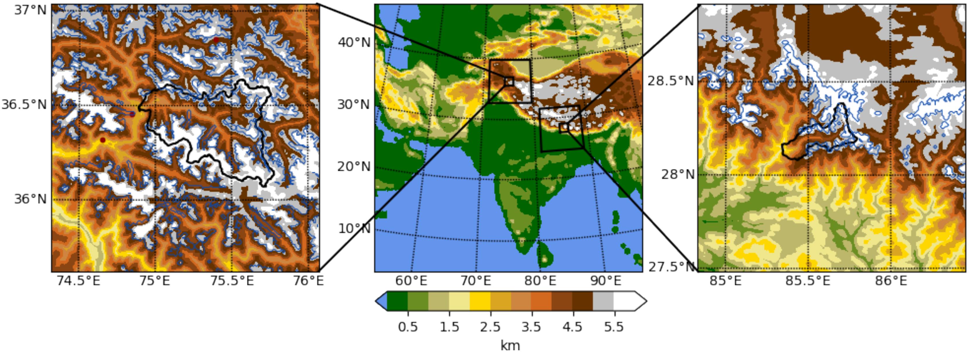
Figure 1. The outer domain (D1, 25 km, middle panel), with its nests. Left panel shows the 1 km domain of Shimshal catchment (D3), and right panel 1 km domain of Langtang catchment (D5). The catchment outlines are indicated by black contours and glacier outlines of GLDAS dataset (Rodell et al., 2004) by blue contours.

The second catchment is the Langtang valley (∼600 km²), located in the central Himalaya, 70 km north of Kathmandu (Nepal) and ranges in altitude from 1406 to 7180 m a.s.l. This valley is U-shaped upstream, while V-shaped downstream. Twenty-four percent of the catchment is glacierized and the average glacier size is 2 km² (Collier and Immerzeel, 2015). Glacier tongues are generally debris-covered (32 km²). Most precipitation (>70%) falls during the monsoon period and glaciers have simultaneous accumulation and ablation during this period (Immerzeel et al., 2014).

Model

We used the advanced research WRF model version 3.8.1 (Skamarock et al., 2008) to simulate the period from January 2011 till January 2014, excluding 1 month of spin up (December 2010). In total we simulate 3 years, to get insight into inter-annual variability. This period is chosen such that no El Niño events are included in the simulation, as they are associated with positive precipitation and temperature anomalies (Syed et al., 2006). The outer domain is showed in Figure 1 and has two nests for each catchment, with resolutions of 5 and 1 km, respectively. All domains have 50 terrain-following vertical levels, stretching from the surface to 50 hPa, with ∼11 levels in the lowest km above the surface. The outer domain is forced with 6-hourly ERA-Interim data (0.75° × 0.75°, Dee et al., 2011), and grid analysis nudging is applied to the horizontal wind, water vapor mixing ratio, and potential temperature fields in the highest 15 vertical levels. Since we are running a 3-year simulation, grid analysis nudging is employed to constrain large-scale circulation (Bowden et al., 2013). We used the same nudging coefficients as Collier and Immerzeel (2015), since that improved the simulated monsoon precipitation for a similar domain as tested in previous work (Collier and Immerzeel, 2015). The model configuration and parameterizations are similar to the ones described in Bonekamp et al., (2018) and are shown in Table 1.

TABLE 1

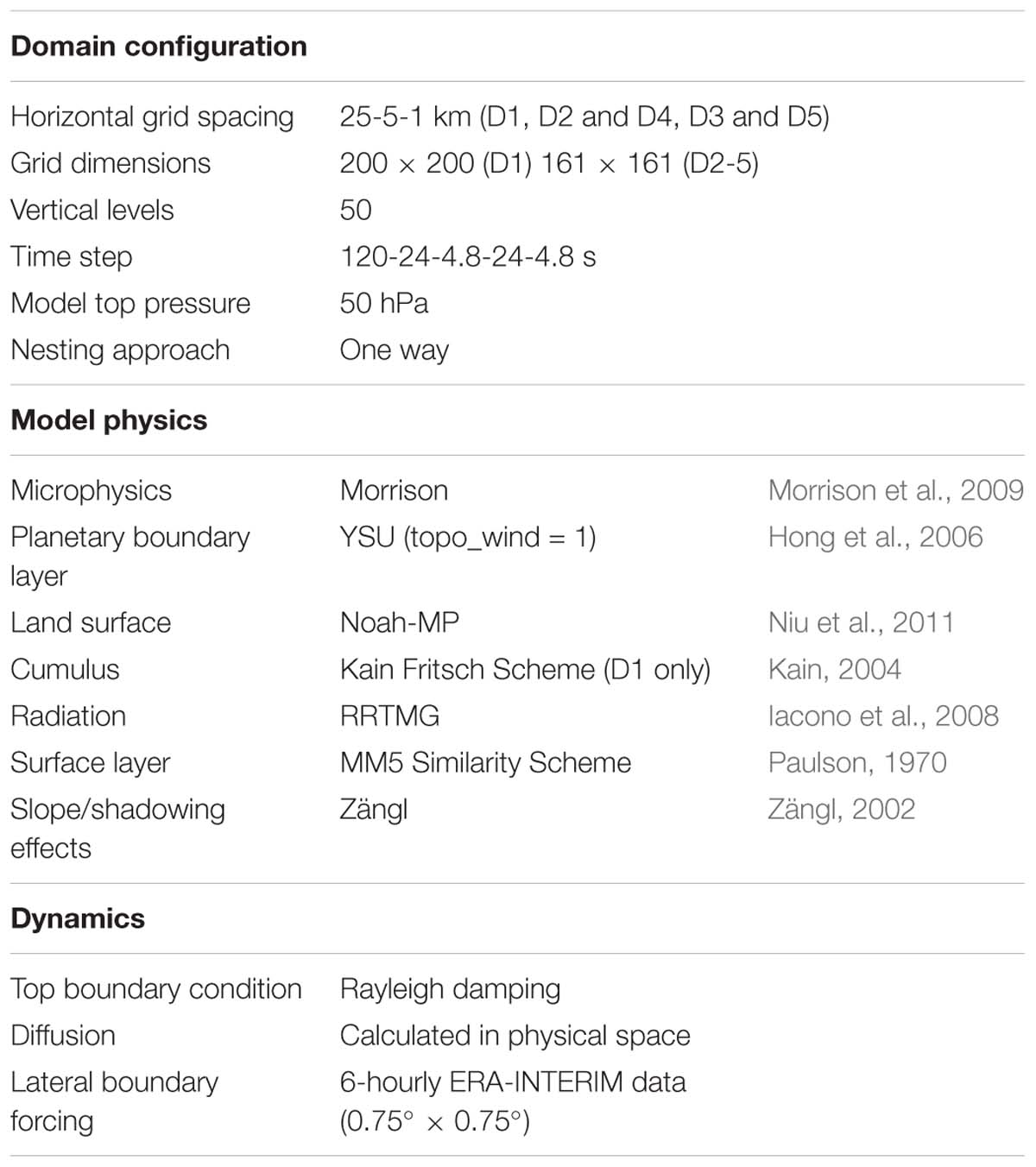
Table 1. Overview WRF configuration.

The default land cover map in WRF is not representative for the region and underestimates both the glacier and forest area (Bonekamp et al., 2018). As the correct representation of land-use is very important for the SEB and thus the valley climate, the land cover dataset is updated using the climate change initiative dataset (CCI; Defourny et al., 2017) of the European Space Agency (ESA), which has a spatial resolution of 300 m.

We initialized the soil moisture, soil temperatures and skin temperatures with the GLDAS (global land data assimilation system) dataset (0.25° × 0.25°; Rodell et al., 2004) as the ERA-Interim initial conditions are unrealistic, in particular the snow depths. The snow height is limited by the amount of snow water equivalent available at each grid point in the GLDAS dataset. The topography is smoothed in D3 only, at a total of eight grid points to reduce numerical instability. The affected grid points are located outside of the studied catchments. WRF simulations are compared to observations for the Langtang catchment in Bonekamp et al. (2018), however, not explicitly for the Shimshal catchment, since those measurements are very limited and the quality is low.

The simulation was performed on the Cartesius cluster of the SURFsara Supercomputing Center¹ on 192 processors and took approximately 55 days to complete.

Glacier Mass Balance

The SMB of a glacier is the sum of all processes adding mass (accumulation) and removing (ablation) mass from the glacier surface over a 1-year period. In our approach, we approximate the glacier mass balance by the difference between snowfall and melt (including refreezing). Melt and refreezing are computed at hourly intervals from the residual in the SEB for all glacier cells, which are designated as clean ice, using the terms calculated by the Noah-MP land surface model (Niu et al., 2011):

$$\text{SEB}={\text{SW}}_{\text{in}}-{\text{SW}}_{\text{ref}}+{\text{LW}}_{\text{in}}-{\text{LW}}_{\text{out}}-\text{SHF}-\text{LHF}+\text{GHF}\left(1\right)$$

Incoming shortwave (SW_in) and longwave radiation (LW_in), outgoing longwave radiation (LW_out), as well as the sensible (SHF), latent (LHF) and ground heat fluxes (GHF), are direct WRF output. The reflected shortwave radiation (SW_ref) is calculated using the simulated surface albedo. Fluxes directed away from the surface are defined as negative. The GHF is driven by the temperature gradient between the surface and the upper soil layer, the upper layer thickness and the thermal conductivity (Niu et al., 2011). If the surface temperature exceeds the melting point, the surface temperature is reset to 273.15 K and the excess energy is used to melt snow or glacier ice. In Noah-MP, the snow layer can consist of three layers and a glacier is treated as frozen soil with appropriate values for albedo, surface roughness, and heat conductivity. In the snowpack and glacier, processes such as refreezing, retention and percolation of melt water and densification are modeled (Niu et al., 2011). This method allows us to investigate the contribution of individual energy balance components to the residual flux. The Pearson correlation coefficients are calculated with 5-day averaged data and the interannual variability is calculated as the standard deviation of each variable.

Our approach involves one-way and offline mass balance modeling (Eq. 1), however, we do implicitly include the feedbacks between the glacier surface and the atmosphere, since those processes are treated by Noah-MP. Since the ground flux accounts for temperature change in the snowpack/ground, there is no need to take the cold content of the snow pack into account for the amount of potential melt in the offline calculations. We assume melt (refreeze) occurs if the residual energy is positive (negative). A snow layer can hold 5% of its volume of water (Pu et al., 2007). We assume that enough liquid water is available in the snow pack or glacier for all negative residual energy to produce a mass gain through refreezing.

Results

Precipitation, Temperature, and Wind

The climates of the central Himalaya and the Karakoram differ considerably. A major contrast between the regions is the precipitation regime: Langtang has a clear monsoon climate, with the highest precipitation amounts during the summer months and a rather dry winter (Figure 2A). Rain dominates the precipitation budget (58%) and falls throughout the year. In January, February, and March a few winter events occur, and precipitation events are more intense than during monsoon. Shimshal, on the other hand, is snow-dominated (92% of the annual precipitation), with most precipitation during the winter months. During the summer months, the monsoon penetrates only episodically into the Karakoram region and provides some rainfall (see section “Origin of Precipitation Events”). This implies that the summers in Shimshal are relatively dry with limited snow accumulation. Seventy-one percent of the snowfall in Shimshal occurs between December and May, compared to fifty-two percent in Langtang. The glaciers in the central Himalaya are therefore simultaneously accumulating and ablating, while glaciers in the Karakoram are gaining mass in winter and melt during summer. Precipitation is variable between years, with potentially large implications for the glacier mass balance (see section “Glacier Surface Mass Balance”).

FIGURE 2

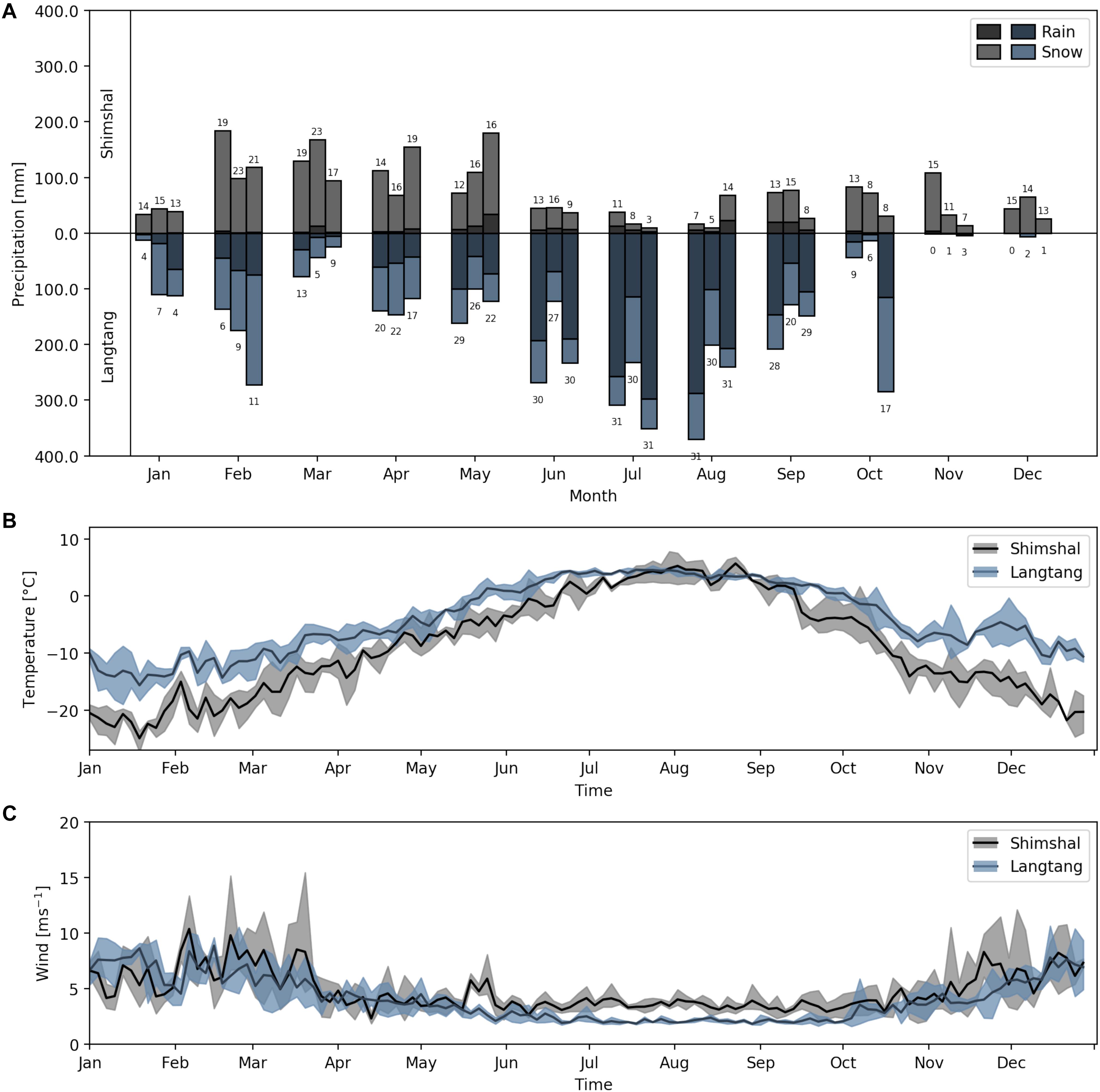
Figure 2. (A) Monthly accumulated catchment-precipitation, with the number of wet days (P > 0.5 mm/day) for 2011–2013 (one bar per year). (B) Five-day catchment average temperature for the Shimshal (black) and Langtang (blue) catchment. (C) as (B) but for the 10-m wind speed. The shading indicates the minimum and maximum value of the individual year.

Shimshal is generally colder than Langtang, with average yearly temperatures of −8.8 and −4.0°C, respectively, and has slightly higher wind speeds on average (4.8 m/s compared to 4.1 m/s in Langtang). Clear similarities in the annual cycle is visible in the two catchments, with the highest temperatures and lowest wind speeds during the summer months (Figures 2B,C).

The precipitation varies with altitude, season, and region. In Figure 3, the seasonal precipitation distribution with altitude is shown for the Shimshal and Langtang catchments. In Langtang, the total annual precipitation is 43% less between 6 and 8 km a.s.l elevation compared to the 2–4 km a.s.l range. The monsoon rain dominates the annual signal, and rain between 2 and 4 km a.s.l altitude is five times higher than between 6 and 8 km a.s.l. Snow between 2 and 4 km a.s.l altitude is 17 times less than between 6 and 8 km a.s.l. The snowfall above 5000 m a.s.l is rather constant with altitude throughout the year. The precipitation peak occurs at the entrance of the Langtang catchment, where the topography blocks the large-scale monsoon winds (Collier and Immerzeel, 2015).

FIGURE 3

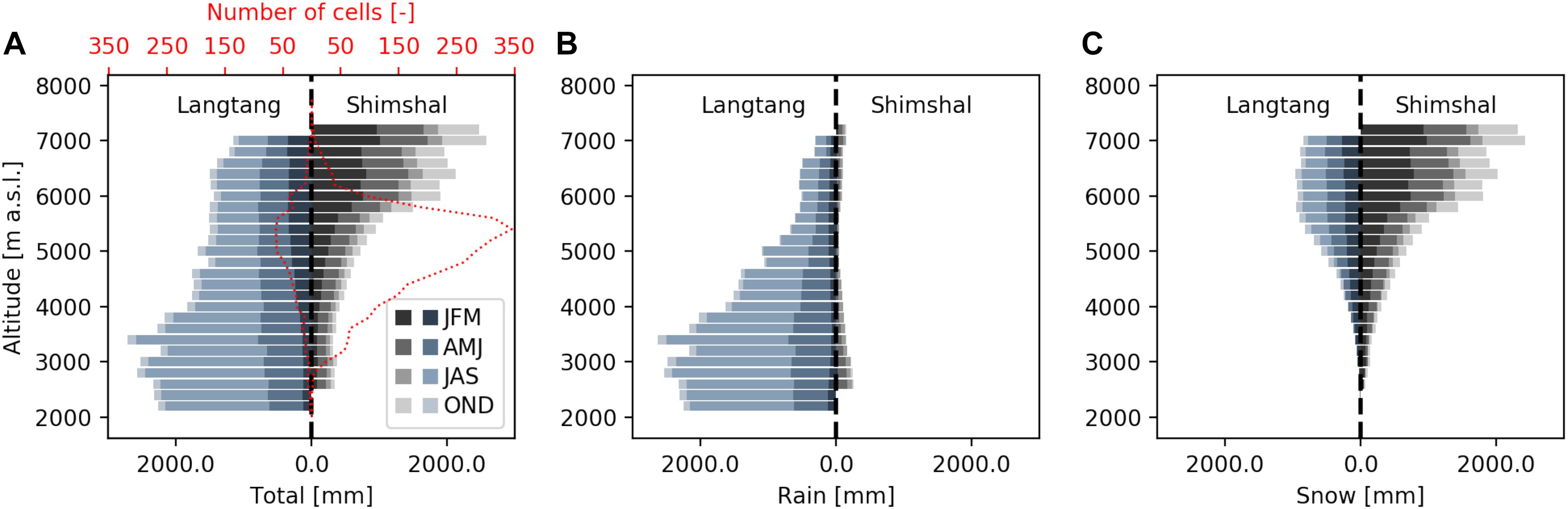
Figure 3. Three-year seasonal average of precipitation (A), rain (B), and snow (C) by 200-m elevation bin. Each bin represents an average of all catchment cells in that altitude range. JFM is the period January, February, March, AMJ is the period April, May, June, JAS is the period July, August, September, and OND is the period October, November, December. The red dotted lines indicate the number of grid cells in each bin for the two catchments (A).

In Shimshal an increase of total precipitation with altitude is observed. The total precipitation is 6 times larger, and snow even 13 times larger, between 6 and 8 km a.s.l than between 2 and 4 km a.s.l. Rain decreases with altitude, as in Langtang, and is 40% lower between 6 and 8 km a.s.l than between 2 and 4 km a.s.l. In Shimshal, 80% of the total snow falls above an altitude of 5000 m a.s.l, while this is only 35% in Langtang.

In summary, in Shimshal, snow dominates the precipitation budget, and the total annual signal shows a positive gradient with altitude, while in Langtang the budget is rain-dominated and the precipitation signal is negative with altitude, consistent with monsoon precipitation peaking at lower altitude than westerly driven precipitation (Immerzeel et al., 2014; Collier and Immerzeel, 2015). Whether the dominant type of precipitation is snow or rain, caused by different circulation systems, is therefore associated with the reverse precipitation gradient with altitude found in Collier and Immerzeel (2015). These results agree with (Hewitt, 2005), who found a fivefold to tenfold increase in precipitation the Karakoram between 2500 and 4800 m a.s.l. Winiger et al. (2005) estimated that snowfall above 4000 m a.s.l ranges from 1000 mm to more than 3000 mm, and that above 5000 m a.s.l altitude, >90% of the precipitation is snowfall, while at lower altitudes >90% of the total precipitation is rain.

Origin of Precipitation Events

The origin of precipitation events is an important unknown in the Karakoram, as both westerlies and monsoon winds influence this region. In this research we propose a simple method to classify the origin of precipitation events in the Karakoram. It would be interesting to combine WRF with a moisture tracking model to fully understand the precipitation sources during the monsoon in the Karakoram (Tuinenburg et al., 2012; de Kok et al., 2018). However, this goes beyond the scope of the present study.

During the winter months (January–March), moisture is transported from west to east, with highest precipitation intensities in the west (Figure 4). Two precipitation bands are clearly visible, which follow the topography clearly. In those months, snow is the dominant precipitation type.

FIGURE 4

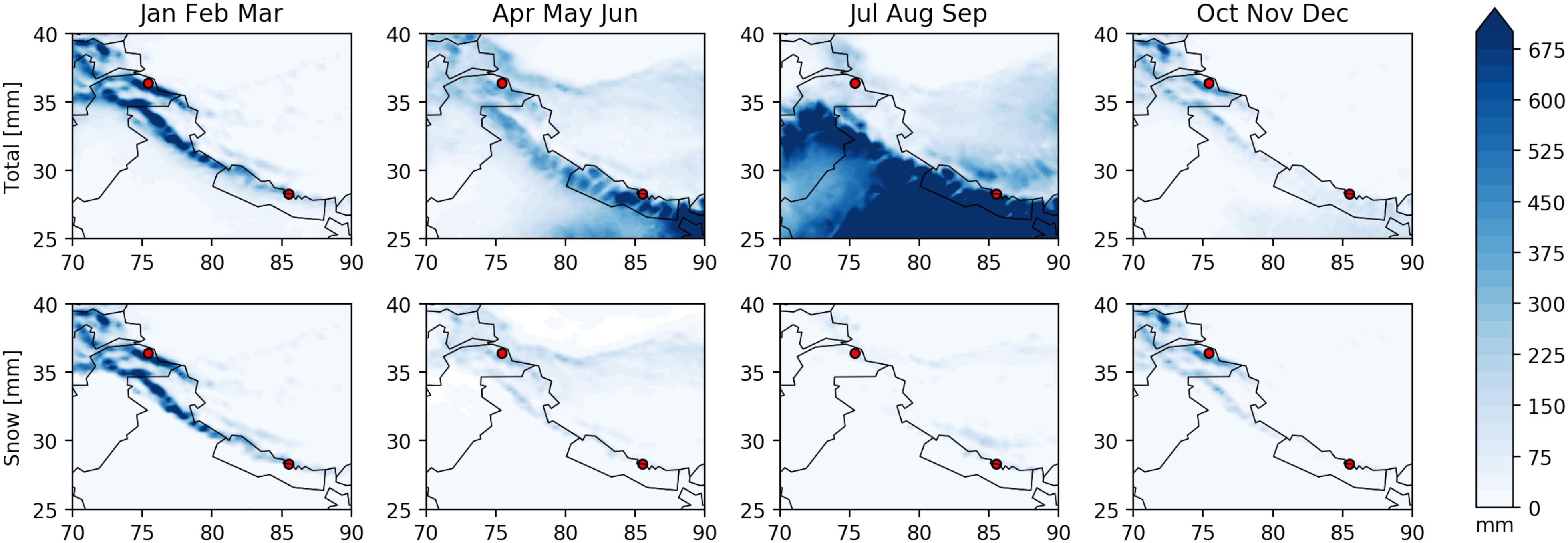
Figure 4. Three-year-averaged seasonal total precipitation (upper panels) and solid precipitation (lower panels) for a subset of the 25-km resolution domain. Black contours indicate country outlines and the red markers the Shimshal (left) and Langtang (right) catchment.

During the summer months (July–September), the monsoon influence is increasing with longitude and it also has a strong south-north decreasing gradient (Figure 4). During those months, snow falls predominantly at high altitudes (>5000 m a.s.l; see Figure 3). In general, moisture is transported from lower to higher latitudes by monsoon winds and provides almost daily precipitation in the central Himalaya.

To investigate the influence and occurrence of the Indian summer monsoon precipitation events in the Karakoram region, the precipitation events with the associated moisture flux and moisture flux direction during the summer period for three different areas are plotted in Figure 5. The precipitation events in box 1, representing the Shimshal catchment, are categorized by the moisture flux direction in box 2, south of Shimshal (75E; 31N). Box 2 is chosen due to its location at the foot of the Himalaya, where winds are generally flowing parallel to the topography and giving a clear separation between monsoon winds (between 40° and 170°) and westerly winds (larger than 170° and smaller than 40°). Box 3 is chosen due to its location in the Karakoram that acts as a funnel for westerly winds.

FIGURE 5

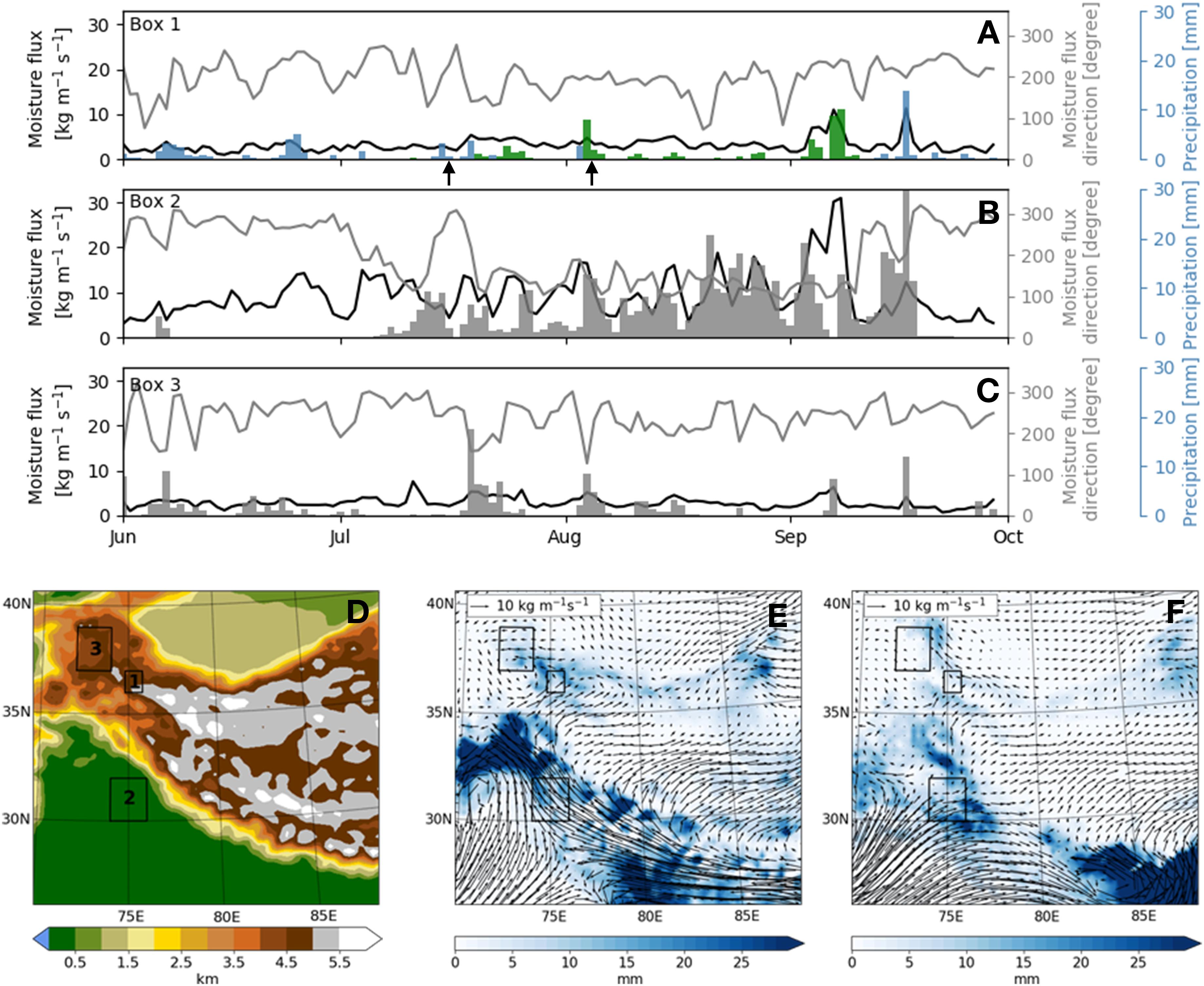
Figure 5. Panels (A–C) show for three different boxes for the months June–October 2012 the daily averaged vertically integrated moisture flux (black), daily averaged moisture flux direction (gray), and daily sum of precipitation (bars). Box 1 (A) represents an average around the Shimshal catchment (75.3E; 36.5N), box 2 (B) is positioned in a monsoon source area (75E; 31N), and box 3 (C) in a westerly source area (73E; 38N). In panel (D) the topography and the position and extent of the boxes is shown. The source of the precipitation events in box 1 are categorized and a green color indicates the precipitation event is monsoon-driven, while a blue color westerly driven. In panel (E) the daily averaged vertically integrated moisture flux (arrows) and daily averaged accumulated precipitation (blue) for a monsoon categorized event (August 04, 2012) for the area same as in (D). Panel (F) is similar to panel (E), but for a westerly categorized event during the monsoon (July 15, 2012). The arrows in (A) indicate the timing of the events used in (E,F).

During the monsoon, the dominant moisture flux direction during a precipitation event is southwest in Karakoram, while the origin of precipitation differs. In other words, it is possible that the direction of the moisture flux as a result of the interaction with the topography during a precipitation event in monsoon is southwest, but that it has a westerly source. The moisture flux direction in the Shimshal catchment (Figure 5A) does not give information directly about the origin of the precipitation events due to the complex topography that creates regional meteo-climatic regimes. The three different boxes are used to track the large scale forcing and therefore origin of the precipitation events. A precipitation event in Shimshal (box 1, Figure 5A) is classified as monsoon event if the integrated moisture flux in box 2 is between 40° and 170°, and classified as westerly event if the moisture flux direction is smaller than 40° or larger than 170° (Figures 5A,B). Based on this characterization, the monsoon period in the Shimshal catchment starts in July and ends halfway September and agrees well with other studies (Lau and Yang, 1997). In the 3-year simulation, on average 22 days with precipitation above 0.5 mm/day occurred between June 1 and August 31. Two third of these events are classified as direct monsoon incursions, an example of which is shown in Figure 5E, and one third from other origins.

Precipitation and moisture fluxes clearly follow the topography. During the winter the westerly disturbances split due to the Hindu-Kush and Pamir mountain ranges, and during summer months the monsoon penetrates deepest in the Karakoram where the topography is lowest. However, this categorization based on the moisture direction in one specific box is rather simple and depends on our selected range of moisture flux direction. Although it works well and provides a clear indication of the large-scale origin of precipitation in the Karakoram, some specific circulation patterns may be missed. An example is shown in Figure 5F, where a monsoon event is wrongly categorized as westerly event and gives noise in the signal.

Glacier Energy Balance

There are clear differences in the simulated surface energy dynamics between the two catchments. The relative contribution of the different terms in the SEB of a glacier controls how sensitive a glacier is to changes in climate, such as increasing temperatures and changing cloud coverage. In Figure 6 the individual energy balance components, as well the residual flux of all glacier grid cells in the Shimshal and Langtang catchments are shown. In Figure 7 the average contribution of each of the individual energy balance components to the residual flux for the months May–September are given to indicate the main drivers of the melt signal.

FIGURE 6

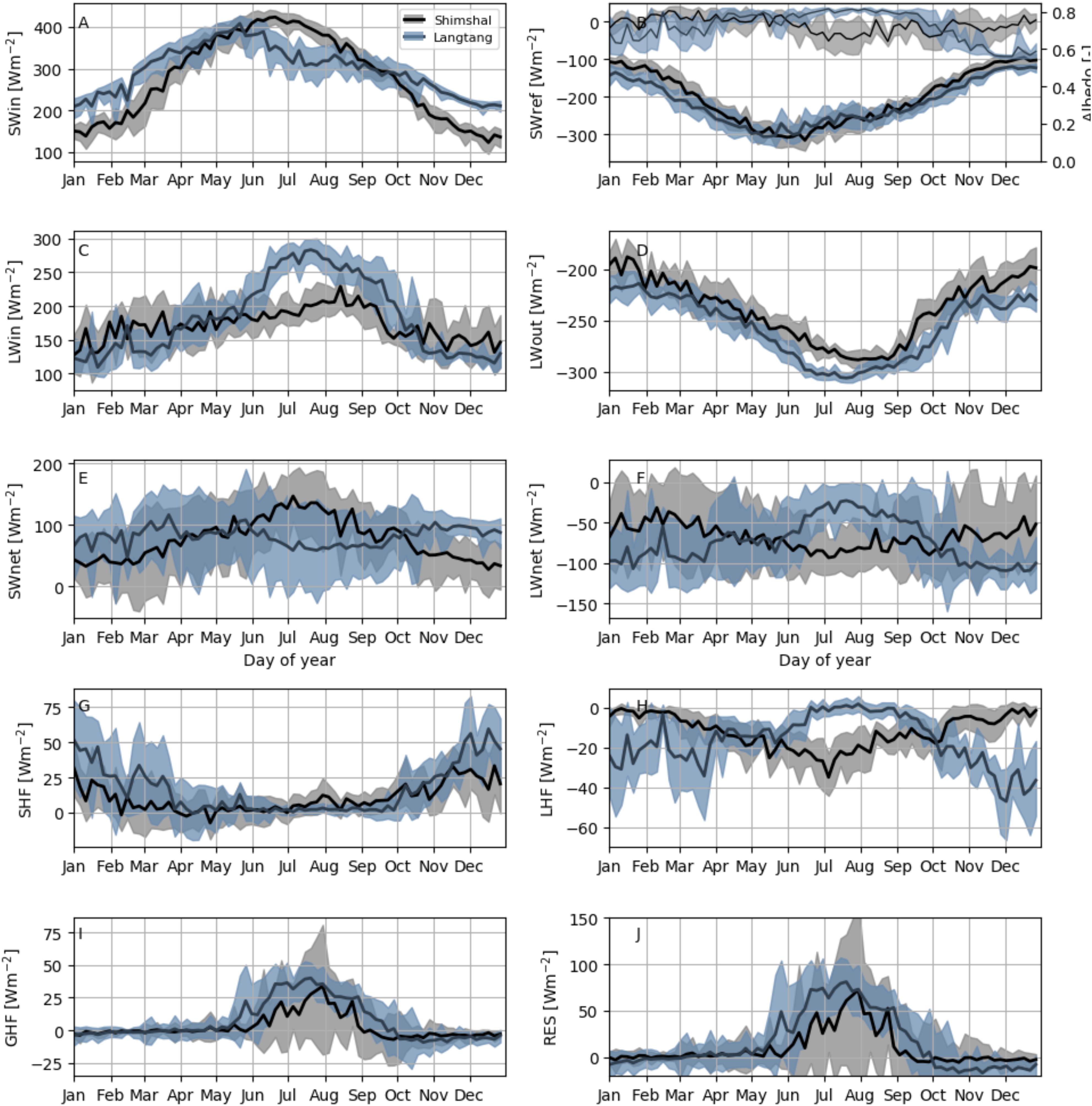
Figure 6. The surface energy balance (SEB) components, 5-day averaged, 3-years average for the glacierized cells in Shimshal (black) and Langtang (blue). The shading indicates the lowest and maximum value of the individual year. SWin (A) and LWin (C) are the short and longwave incoming radiation components, SWref (B) and LWout (D) the shortwave reflected and longwave outgoing radiation components, and SWnet (E) and LWnet (F) the net radiation components. SHF (G), LHF (H), and GHF (I) are the sensible, latent, and ground heat flux, respectively. The albedo is plotted in panel (B) (thin lines). The residual term (RES, Panel J) is calculated as SWnet + LWnet + SHF + LHF + GHF.

FIGURE 7

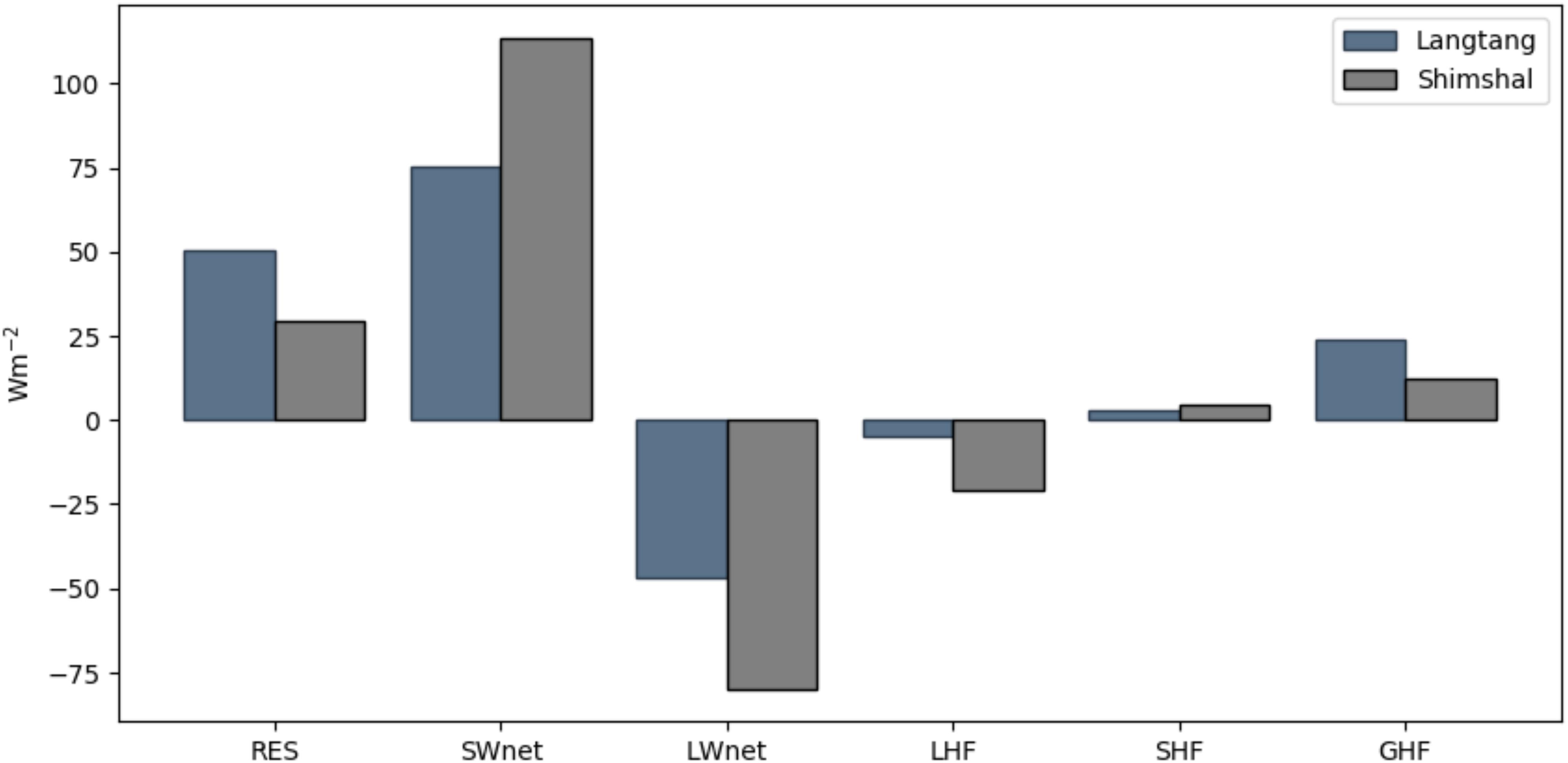
Figure 7. The average residual flux (RES), shortwave net (SWnet), longwave net radiation (LWnet), latent heat flux (LHF), sensible heat flux (SHF), and ground heat flux (GHF) for all glacierized cells in Langtang (blue) and Shimshal (gray) for the three melt seasons (May–September).

The net shortwave radiation provides the largest energy input at the surface (Figures 6, 7) and, due to a lower and more variable surface albedo, its variations correlate (Pearson correlation) most strongly with those of melt in Shimshal (r = 0.79 ± 0.01). Conversely, the net longwave radiation dominates the melt signal in the Langtang (r = 0.76 ± 0.02), due to greater cloud cover and higher atmospheric humidity during the monsoon. The net longwave radiation itself is negative, but variations in this flux have the strongest influence on the residual flux in Langtang. The absolute values of the sensible, latent and GHF are low compared to the shortwave and longwave radiation components (Figure 6). However, the latent heat flux could also be an important contributor to the regional differences in the residual flux and thus glacier melt, as it shows the opposite temporal pattern in the two regions (Figure 6H). During the melt season, the LHF is almost zero in Langtang (r = −0.83) due to high relative humidity, while in Shimshal this flux is larger and negative (r = 0.43) due to relatively dry conditions during summer, and indicating that significant amounts of energy are extracted from the surface by sublimation and evaporation. Previous estimates have shown that snow sublimation in Langtang could account for 21% of the loss of the total snowfall (Stigter et al., 2018). For the Karakoram, however, no studies have been done to quantify the effects of sublimation. Understanding regional and seasonal differences in the LHF could therefore be important to understand the glacier mass balance anomaly in detail.

The variation in the residual flux is more pronounced at Shimshal, mainly due to variability in the surface albedo, which is infrequently increased by a small number of snow events during the melt season. The surface albedo influences the shortwave reflected radiation and is mainly influenced by the age of the snow pack on the glacier. In Langtang, however, snow events happen on a daily basis at high altitude, resulting in a consistently higher surface albedo (Figure 6B). The surface albedo resets to the albedo of fresh snow in the Noah-MP land surface model (0.84) when fresh snow covers the old layer by a depth of at least 10 mm. Due to the land surface model treatment of glacier surfaces as being permanently snow covered, glacier surface albedo ranges between 0.6 and 0.84 for both catchments throughout the year (Figure 6B). The importance of the albedo effect is expressed in the fact that the shortwave incoming radiation is much higher in Shimshal during summer, while the reflected shortwave radiation of Shimshal and Langtang is comparable. The summer months in Langtang are generally cloudy with large variability in shortwave incoming and therefore net radiation as a result.

Clouds influence the SEB mainly by emitting longwave radiation (thin high clouds warm the surface) and blocking the incoming shortwave radiation (low thick clouds cool the surface) (Twomey, 1991). However, since clouds in a cold climate are colder and less optically thick, the warming effect of high-level clouds is small in cold regions. In Langtang, low- and high-level clouds are present during the monsoon and lead to a decrease in incoming shortwave radiation and an increase in incoming longwave radiation (see Figures 6, 8). In Shimshal, low-level clouds occur during the winter months and decrease the shortwave incoming radiation. Therefore, clouds impact the energy balance components and represent an important driver for the differences in the glacier energy balance between Shimshal and Langtang.

FIGURE 8

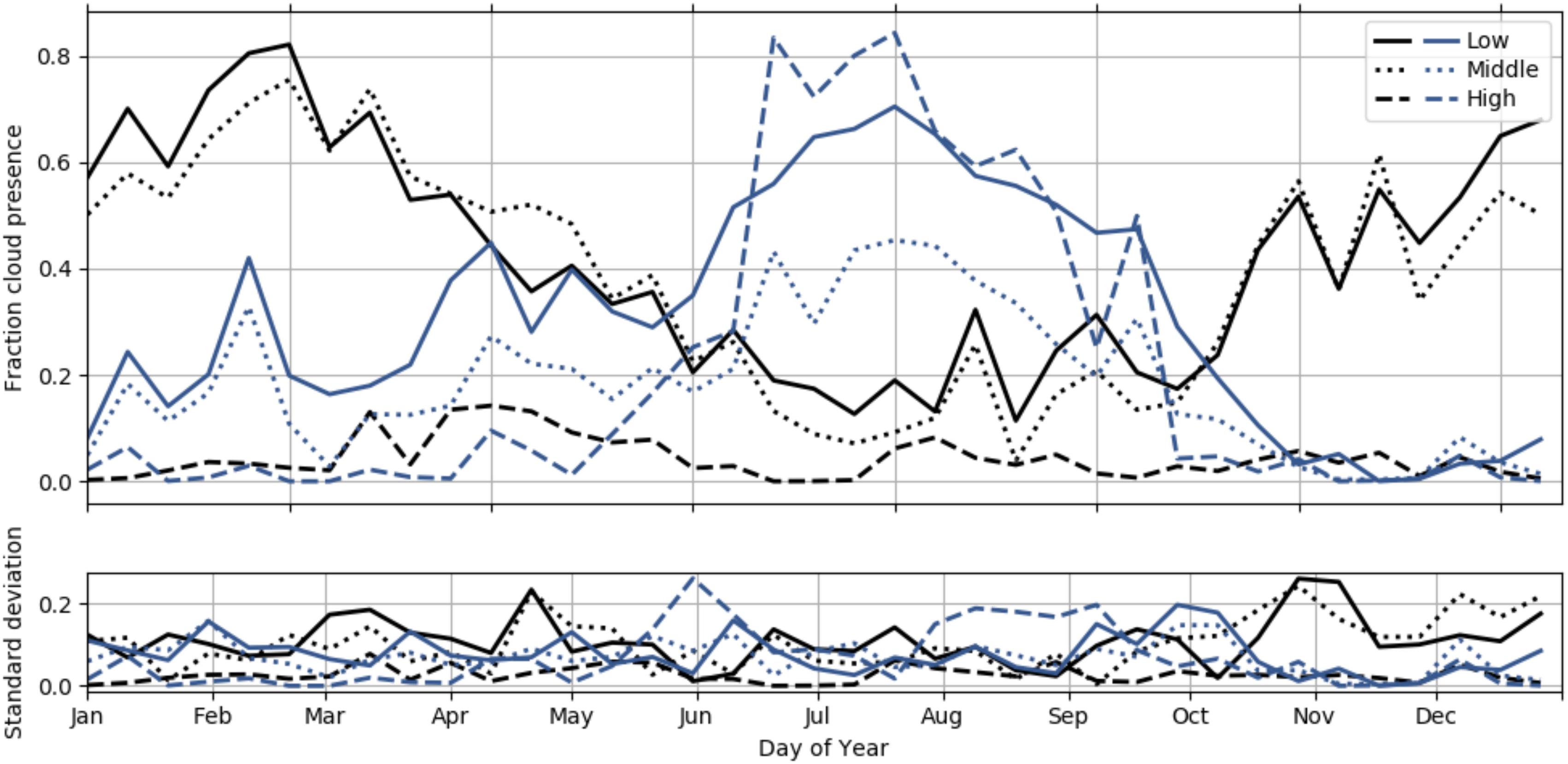
Figure 8. Fraction of glacierized cells which are covered by high- (>6 km a.s.l) middle- (2–6 km a.s.l) and low (<2 km a.s.l) clouds (upper panel). The lower panel indicates the standard deviation of the average values. Altitudes are indicated as altitude above the surface. Three-years averaged for Langtang (blue) and Shimshal (black).

The residual flux at sub-daily time steps provides information about the melt and refreezing cycle of glacier cells in the two different regions. The differences in timing of the melt peaks are caused by the latitudinal differences of the two catchments. In the yearly averaged diurnal cycle of the residual flux, Langang has a higher residual-energy peak than Shimshal (Figure 9). In Langtang and Shimshal, average melt fluxes of 17.7 and 11.3 Wm⁻², respectively, are observed. Our calculations assumed that the negative residual flux is used for refreezing of melt water and liquid precipitation. Based on this assumption, the amount of refreezing on a yearly basis could amount to 60 and 52% of the total melt in Langtang and Shimshal, respectively. Calculations with station data in the Langtang catchment show refreezing in a snowpack can be up to 43% of the total snow melt (Stigter, 2019 personal communication). However, those calculations neglect rain as liquid water input and assume refreezing is water-limited, since the snow pack is shallow and can hold maximum of 10% of its mass as liquid water. Therefore, the amount of refreezing calculated in this paper is likely overestimated, which is discussed in more detail in Section “WRF Caveats.”

FIGURE 9

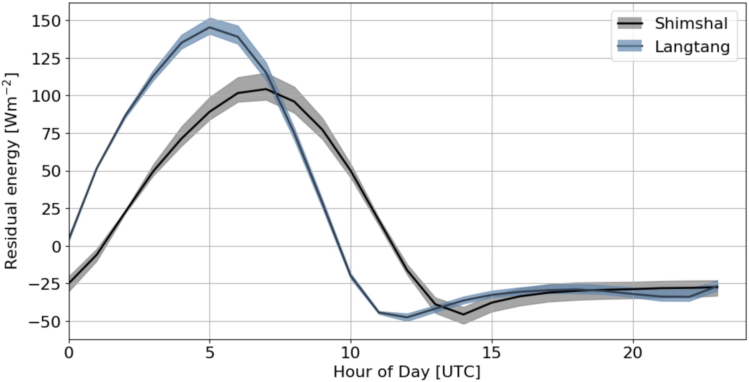
Figure 9. Diurnal cycle of the residual flux for Shimshal (black) and Langtang (blue). The shading indicates the interannual variability.

Glacier Surface Mass Balance

In Figure 10, the SMB, snow melt and snow accumulation are shown for all glacier cells in the inner domains for each year separately.

FIGURE 10

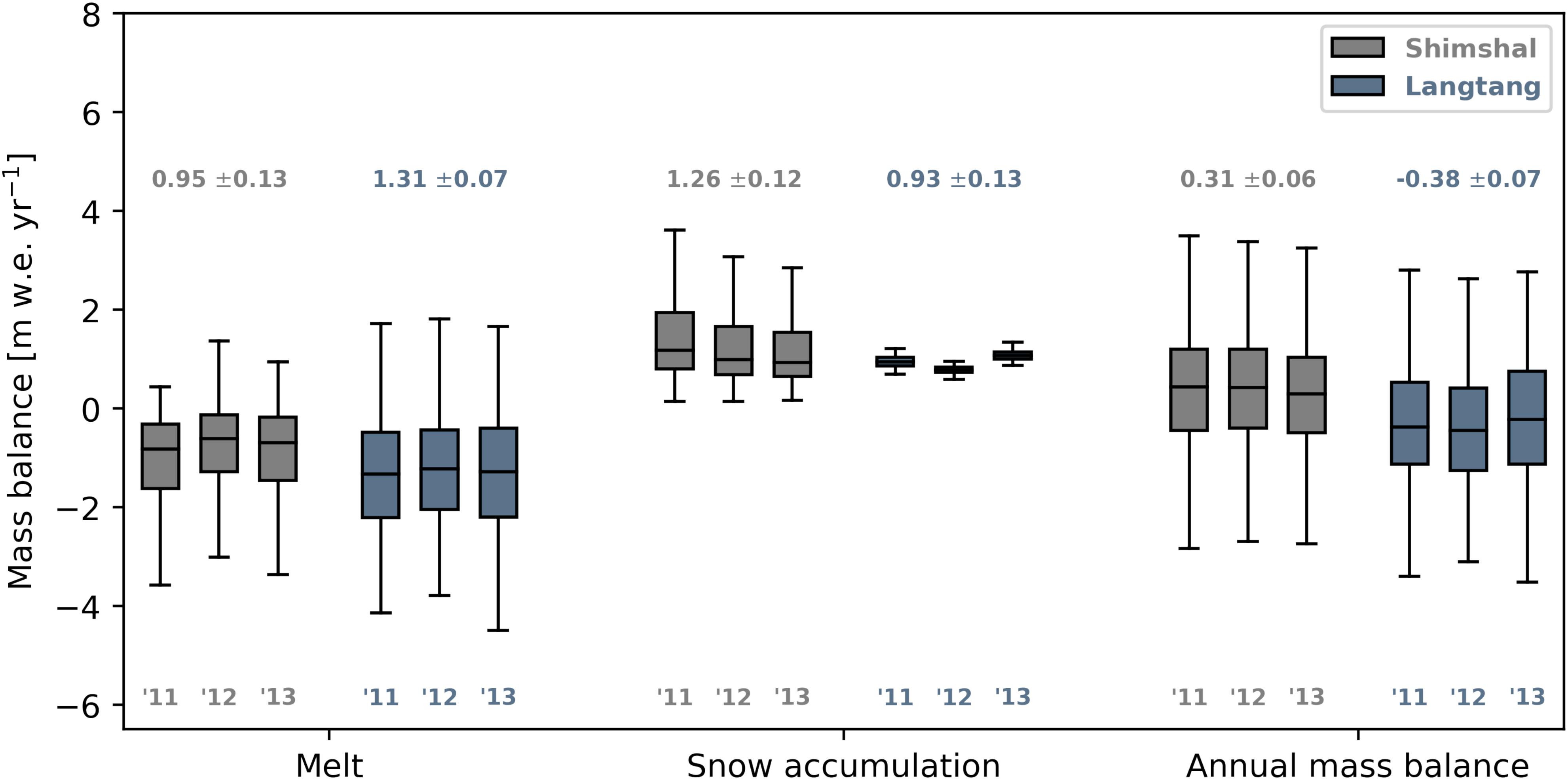
Figure 10. Box plots of the effect of the melt and snow accumulation on the glacier surface mass balance, and the annual mass balance for each simulated year shown for Shimshal (gray) and Langtang (blue). The 3-yearly mean and standard deviation is shown above the boxplots for each category and catchment.

The melt is lower in the Shimshal catchment, but more variable (σ = 0.13 m w.e. year⁻¹) than in Langtang (σ = 0.07 m w.e. year⁻¹). This variability originates from the shortwave variation in particular (cf. section “Glacier Energy Balance”). However, another important driver for the difference in mass balance between the catchments is the amount of snowfall, which leads to a positive mass balance in Shimshal (1.26 m w.e. year⁻¹ snowfall). In Langtang the snow amount (0.93 m w.e. year⁻¹) does not compensate for melt (−1.31 m w.e. year⁻¹) and the mass balance is negative for the majority (63%) of the glacier cells. The variability in snow accumulation is much higher in Shimshal than in Langtang, likely due to the erratic nature of snow storms produced by westerly disturbances in Shimshal, while snowfall at high-altitude in Langtang is more constantly driven by monsoon precipitation. This result suggests that the variability in the mass balance in Langtang is mainly controlled by spatially variable melt, rather than snow fall.

In Figure 11, the average SMB per altitude bin is shown. The different sign in the mass balances of Langtang (−0.40 m w.e. year⁻¹) and Shimshal (0.31 m w.e. year⁻¹) shows the vertical glacier mass balance profile is different in the central Himalaya and the Karakoram region. The residual energy at lower altitudes shows a strong interannual variability in Shimshal, which indicates that the melt on the glacier tongues varies strongly. However, the number of glacier cells is low (<5) at low elevations (<4400 m a.s.l) and could explain the sensitive signal as well.

FIGURE 11

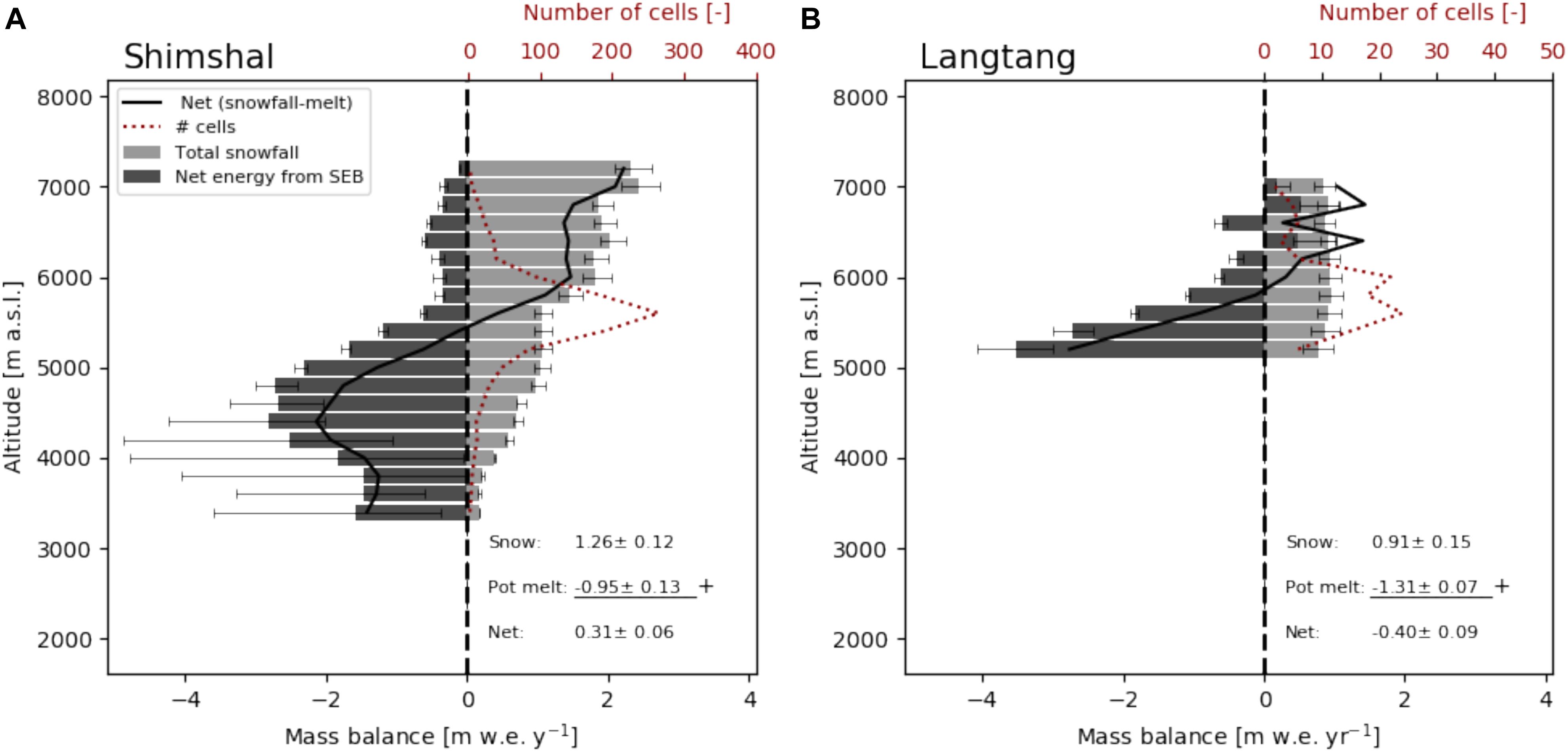
Figure 11. Normalized mass balance (black line) with altitude for Shimshal (A) and Langtang (B). Snow (light gray) and melt caused by residual energy (dark gray). Each bin represents an average of that altitude range. The red dashed line indicates the amount of cells. Error bars indicate the variability between simulated years. Numbers indicate the average snow (snow), residual energy flux (pot melt), and total mass balance (net) over 2011–2013.

In the Langtang catchment, glaciers are relatively small and located in a small altitude range (5200–7000 m a.s.l). 17.9% of the catchment is a clean-ice glacier and 59% [accumulation area ratio (AAR) is 0.41] of the glacier points is located below the equilibrium line altitude (5900 m a.s.l), indicating relatively high melt rates. The Shimshal catchment is glacierized by clean-ice glaciers over 37.4% of its area, contains larger glaciers, and has a large accumulation (>5500 m a.s.l) and ablation zone (<5500 m a.s.l). Shimshal contains big glaciers, which originate at higher altitude, and accumulation is possible due to large amounts of snow and low melt rates. The AAR is 0.61, which leads to a positive mass balance when all glacier cells are averaged.

Discussion

Model Performance

The simulated mass balance for years 2011–2013 in Langtang of −0.40 ± 0.09 m w.e year⁻¹ is in agreement with previously reported values. Baral et al. (2014) estimated the mass balance of Yala glacier in the Langtang catchment (November 10, 2011 to November 03, 2012) to be −0.89 m w.e. year⁻¹. Pellicciotti et al. (2015) estimated the average mass balance of four glaciers in the Langtang catchment (with only non-debris parts of the glacier taken into account) at −0.32 ± 0.18 m w.e. year⁻¹ between the years 1974–1999. Ragettli et al. (2016) found a similar number for debris-free glaciers −0.38 ± 0.17 m w.e. year⁻¹, which is an ensemble mean between the years 2006 and 2015.

For the Karakoram region, previous studies report both positive and negative mass balances (a selection is provided in Table 2). Our calculated mass balance for Shimshal is comparatively high (+0.31 ± 0.06 m w.e. year⁻¹). Previous studies have found stable and positive mass balances in the central and northeastern part of the Karakoram and negative mass balances in the west (Groos et al., 2017). However, they have also reported high-spatial variability, indicating that regional averages could give a distorted view.

TABLE 2

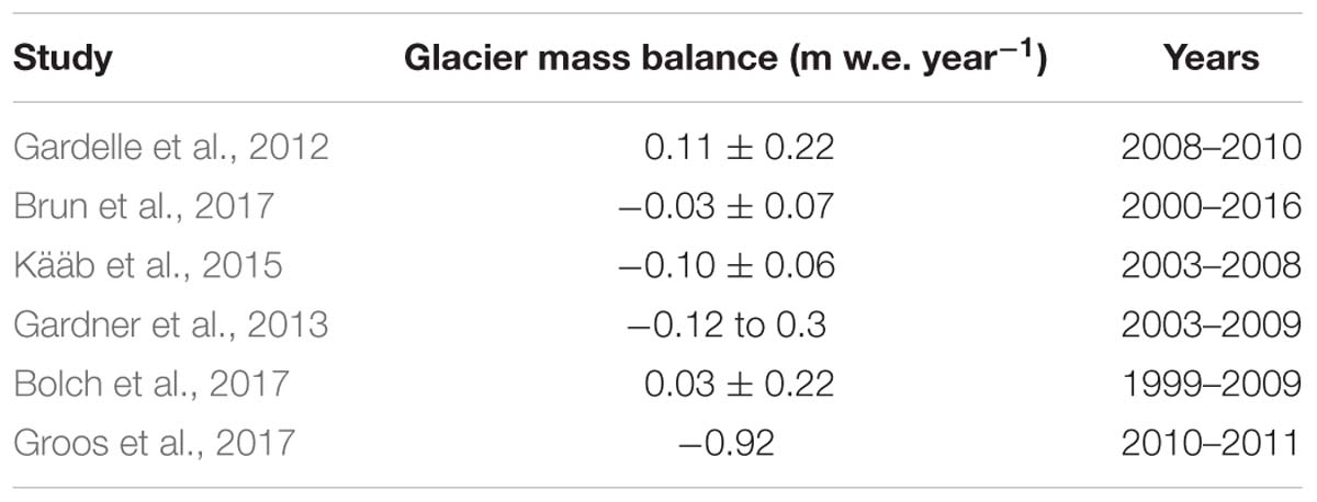
Table 2. Overview of selected mass balance studies in the Karakoram.

Examining individual glaciers, for example, the Yazghil glacier gained ±5 m, Malungutti 5–10 m and Khurdopin 15–20 m in thickness between the years 1997 and 2001 (Hewitt, 2005). These observations suggest accumulation rates of more than 1 m w.e. year⁻¹ may be reasonable for this region. However, we note that due to the cold bias in WRF for High Mountain Asia (Bonekamp et al., 2018), the estimation of snowfall could be overestimated.

In our study WRF appears to reproduce regional differences in glacier mass balance compared to previous studies. Critical is the high spatial resolution as shown in Collier and Immerzeel (2015), Groos et al. (2017), and Bonekamp et al. (2018). The spatial resolution of the model is also important to explicitly resolve local conditions at the glaciers, especially outside the Karakoram region, where relatively small glaciers are present. However, results in this paper exclude the smallest glaciers, due to the grid spacing of 1 km. In general catchments and glaciers are larger in the Karakoram than in central Himalaya, and we note that the differing catchment sizes of Shimshal and Langtang may impact the altitudinal gradients presented. Nonetheless, our results are consistent with previous studies that investigate the Karakoram anomaly and show the importance of winter snow accumulation (Archer and Caldeira, 2008), lower summer temperatures and more (solid) summer precipitation (Fowler and Archer, 2005), and less net radiation (de Kok et al., 2018) that favor the Karakoram anomaly. Unfortunately, our study does not provide data with which any of these hypotheses could be tested due to the time frame.

A limitation of our work is that we only take clean ice glaciers into account and therefore the melt could be overestimated assuming the debris has a net insulating effect. However, the role of this insulation in debris-covered glaciers is still unclear, since the two types of glaciers seem to experience very similar melting rates (Pellicciotti et al., 2015; Brun et al., 2018). Currently, there are two hypotheses that try to explain the relatively high melting rates in debris-covered glaciers: the first is that high-melt rates at ice cliffs compensate for the low-melt rates averaged over the debris covered tongues (Pellicciotti et al., 2015). The second hypothesis is that debris-covered glacier tongues have a lower emergence velocity than clean-ice glacier tongues, whereby the similar thinning rates between the two types of glaciers are observed, while melt rates are lower at debris-covered glaciers (Anderson and Anderson, 2016).

WRF Caveats

A major mass input of glaciers is caused by snow-avalanching, especially in the Karakoram region (Hewitt, 1993). Although avalanching is not incorporated in WRF, we still see a positive mass balance in this region, and we conclude glaciers behave differently, even without the avalanching effect. Avalanching would also redistribute snow to lower altitudes, and could bias the simulated glacier mass balance from WRF to high altitudes. To make a better glacier mass balance estimation, glacier accumulation area outlines should be included to estimate the snow accumulation available from avalanching.

Snow drift and wind-blown redistribution of snow are also a major contributor to the glacier mass balance (Dadic et al., 2010), and are not taken into account in WRF. Similarly, WRF does not include glacier flow, but since glacier extents are not likely to change significantly within a 3-year period, we do not expect large uncertainties, as we consider all glacier cells in the domain.

There are also uncertainties in the treatment of glacier surfaces in the Noah-MP land-surface model. The main issue is the imposition of a minimum snow depth on glaciers often leads to an overestimate of albedo during the ablation season, which impacts local meteorological conditions on the glaciers (e.g., Collier et al., 2013). The treatment of glaciers as fully saturated and fully frozen soil surfaces in the Noah family of land-surface models is a simplification but has been found to produce reasonable simulations of glacier surface energy and mass fluxes (Mölg and Kaser, 2011).

In our approach, we also assume an unlimited amount of water is available for (re)freezing of water, while in reality the refreezing process will be water-limited, especially during dry and cold periods, when there is no melt, and no precipitation. In WRF, a cold bias is common at high altitudes (e.g., Bonekamp et al., 2018) and will likely influence the amount of snowfall and of melt of glacier surfaces and snow. Both issues likely bias the mass balance positively. The total simulation period of 3 years also gives a limited view of the interannual variability and averages presented, since those 3 years do not represent a climatological period. Furthermore the study period is too short to assess climatic trends that might have caused Karakoram anomaly, and/or glacier mass loss in Nepal.

Several studies have validated the performance of WRF for the Langtang region (e.g., Collier and Immerzeel, 2015; Bonekamp et al., 2018), however, direct observations of high-altitude precipitation are sparse and satellite derived products are of insufficient resolution and quality to capture spatial variation and the magnitude of mountain precipitation (Immerzeel et al., 2015). It is therefore difficult to draw quantifiable conclusions about potential biases at high altitude.

Climate Sensitivity

The annual average temperature in Shimshal is low and the catchment is therefore likely more sensitive to future precipitation rather than temperature shifts. However, with increasing air temperatures, the air can hold more moisture and therefore potentially more precipitation can occur, which favor a positive mass balance (Kapnick et al., 2014). Furthermore, our results show that the longwave radiation is the dominant driver of the variations in the melt signal in Langtang. Hence, besides a decrease in mass balance due to a rise of the equilibrium line altitude, glaciers in Langtang will likely show an enhanced sensitivity to temperature due to the increase in incoming longwave radiation.

Currently, snow events are only sporadic during the melt season in Shimshal (Mayer et al., 2014), leading to lower surface albedo and more energy available for melt compared with Langtang. However, these summer snow events also input mass, reduce the amount of sunshine hours, and increase the albedo (Hewitt, 2005; de Kok et al., 2018). This implies that a change in the number of summer snow events in Shimshal could influence the melt through several processes, with an increase supporting positive mass balance conditions. In contrast, slight changes in summer precipitation amounts affect the melt only marginally in Langtang, since the frequent summer snowfall already results in a high albedo. Hence, the sensitivity of the glacier melt to summer precipitation is higher in Shimshal than in Langtang.

Eventually, changes in large-scale forcing, such as westerly winds, will explain the glacier response only partly, since different glaciers will respond differently to identical changes in external conditions. We have shown that the glacier response is very different in Shimshal and Langtang, owing to a very different distribution of the energy balance. The climate system is complex and each component in it will adapt, aiming for a new equilibrium.

Conclusion

Understanding regional differences of meteorological variables at the catchment scale is key to understand the heterogeneous behavior of glaciers in High Mountain Asia. In this study, we modeled at 25, 5 and 1-km grid spacing two catchments in contrasting climate regions: the central Himalaya and the Karakoram. We show at high-resolution that climate and glacier behavior is spatially highly variable between the Karakoram and the central Himalaya, and that the accumulation and melt dynamics of both regions are different as a result of contrasting meteorological conditions. The interpretation of their impact on the glacier energy and mass fluxes and the elucidation of differences between catchments is novel. To our knowledge, this is the first multi-year simulation at 1-km resolution for regional comparison of catchments in High Mountain Asia and gives a unique data set to investigate catchment-scale atmospheric processes.

Glacier melt is highly variable between years in the Karakoram and its variability is primarily driven by the net shortwave radiation (r = 0.79 ± 0.01), with only limited cloud cover during the melt season. The surface albedo variability drives melt variation, and is strongly influenced by summer snow events in the Karakoram region. The number of snow events during the melt season is more important than the total amount of snow to increase the albedo and thus reduces energy available for melt. This indicates that if the frequency of summer precipitation events will increase in the Karakoram in future due to, for example, a stronger summer Indian monsoon, this will favor the mass balance of Karakoram glaciers. In Shimshal, the latent heat flux also plays an important role in extracting energy from the surface during the comparatively dry conditions during summer. Conversely, in the central Himalaya, variability in glacier melt is driven primarily by net longwave radiation (r = 0.76 ± 0.02), as both high- and low-level clouds dominate the weather during the melt season. This indicates that glaciers in the central Himalaya have an additional sensitivity to air temperature, since the melt signal is dominated by the net longwave radiation (specific humidity and clouds).

In the Karakoram, there is an additional sensitivity to summer precipitation by means of the albedo increase and summer cloudiness. The precipitation sensitivity differs between the Karakoram and the central Himalaya, due to the different precipitation gradients and dominant precipitation type. Although the precipitation sensitivity of glaciers is usually less than the temperature sensitivity (Anderson and MacKintosh, 2012), this might not be the case for Karakoram and summer precipitation.

To understand glacier response to atmospheric conditions a detailed insight into the accumulation and ablation regimes is required and is for the first time done in this study for two contrasting sites in HMA. We show glaciers behave differently in central Himalaya and the Karakoram region, and that the glacier mass balance is sensitive to both the residual flux of the energy balance and snowfall. Annually, 1.26 ± 0.12 m w.e. snowfall in Shimshal occurs compared with 0.91 ± 0.15 m w.e. in Langtang. The residual energy available for melt is lower in Shimshal (−0.95 ± 0.13 m w.e. year⁻¹) compared with Langtang (−1.31 ± 0.07 m w.e. year⁻¹), resulting in positive and negative simulated SMB in Shimshal (+0.31 ± 0.06 m w.e. year⁻¹), and in Langtang (−0.40 ± 0.09 m w.e. year⁻¹), respectively.

Our research implies that the sensitivity of glaciers to climate change is regionally driven and future work could map regions of sensitivity to different components of the energy balance and meteorological forcing fields. This will give a more detailed insight into glacier behavior under climate change, as not all glaciers behave similarly, to rising temperatures. Understanding glacier mass balance anomalies requires quantification and insight in subtle shifts in the energy balance and accumulation regimes at high altitude.

Data Availability

The data are available at https://doi.org/10.5281/zenodo.2611581 (Langtang) and https://doi.org/10.5281/zenodo.2611323 (Shimshal).

Author Contributions

PB and WI designed the study. PB performed the simulations and the analysis with input of WI, RdK, and EC. PB wrote the initial version of the manuscript. RdK, EC, and WI commented on the initial manuscript and helped to improving this version.

Funding

This project has received funding from the European Research Council (ERC) under the European Union Horizon 2020 Research and Innovation Program (Grant Agreement No. 676819) and Netherlands Organization for Scientific Research under the Innovational Research Incentives Scheme VIDI (Grant Agreement No. 016.181.308). EC was supported by the German Research Foundation (DFG) Grant MO 2869/1-1. Supercomputing resources were financially supported by NWO and provided by SURFsara (www.surfsara.nl) on the Cartesius cluster.

Conflict of Interest Statement

The authors declare that the research was conducted in the absence of any commercial or financial relationships that could be construed as a potential conflict of interest.

Footnotes

1. ^ www.surfsara.nl

References

Andermann, C., Bonnet, S., and Gloaguen, R. (2011). Evaluation of precipitation data sets along the himalayan front. Geochem. Geophys. Geosys. 12:Q07023. doi: 10.1029/2011GC003513

CrossRef Full Text | Google Scholar

Anderson, B., and MacKintosh, A. (2012). Controls on mass balance sensitivity of maritime glaciers in the southern alps, new zealand: the role of debris cover. J. Geophys. Res. 117:F01003. doi: 10.1029/2011JF002064

CrossRef Full Text | Google Scholar

Anderson, L. S., and Anderson, R. S. (2016). Modeling debris-covered glaciers: response to steady debris deposition. Cryosphere 10, 1105–1124. doi: 10.5194/tc-10-1105-2016

CrossRef Full Text | Google Scholar

Archer, K. (2008). Historical trends in the jet streams. Geophys. Res. Lett. 35, doi: 10.1029/2008GL033614

CrossRef Full Text | Google Scholar

Baral, P., Kayastha, R. B., Immerzeel Walter, W., Pradhananga Niraj, S., Bhattarai Bikas, C., Shahi, S., et al. (2014). Preliminary results of mass-balance observations of yala glacier and analysis of temperature and precipitation gradients in langtang valley, Nepal. Ann. Glaciol. 55, 9–14. doi: 10.3189/2014AoG66A106

CrossRef Full Text | Google Scholar

Bolch, T., Kulkarni, A., Kääb, A., Huggel, C., Paul, F., Cogley, J. G., et al. (2012). The state and fate of himalayan glaciers. Science 336, 310–314. doi: 10.1126/science.1215828

PubMed Abstract | CrossRef Full Text | Google Scholar

Bolch, T., Pieczonka, T., Mukherjee, K., and Shea, J. (2017). Brief communication: glaciers in the hunza catchment (Karakoram) have been nearly in balance since the 1970s. Cryosphere 11, 531–539. doi: 10.5194/tc-11-531-2017

CrossRef Full Text | Google Scholar

Bonekamp, P. N. J., Collier, E., and Immerzeel, W. W. (2018). The impact of spatial resolution, landuse and spin-up time on resolving spatial precipitation patterns in the himalayas. J. Hydrometeorol. 19, 1565–1591. doi: 10.1175/JHM-D-17-0212.1

CrossRef Full Text | Google Scholar

Bookhagen, B., and Burbank, D. W. (2010). Toward a complete himalayan hydrological budget: spatiotemporal distribution of snowmelt and rainfall and their impact on river discharge. J. Geophys. Res. 115, 1–25. doi: 10.1029/2009JF001426

CrossRef Full Text | Google Scholar

Bowden, J. H., Christopher, G. N., and Tanya, L. O. (2013). Simulating the impact of the large-scale circulation on the 2-m temperature and precipitation climatology. Clim. Dyn. 40, 1903–1920. doi: 10.1007/s00382-012-1440-y

CrossRef Full Text | Google Scholar

Brun, F., Berthier, E., Wagnon, P., Kääb, A., and Treichler, D. (2017). A spatially resolved estimate of High Mountain Asia glacier mass balances from 2000 to 2016. Nat. Geosci. 10:668. doi: 10.1038/ngeo2999

PubMed Abstract | CrossRef Full Text | Google Scholar

Brun, F., Wagnon, P., Berthier, E., Shea, J. M., Immerzeel, W. W., Kraaijenbrink, P. D. A., et al. (2018). Ice cliff contribution to the tongue-wide ablation of changri nup glacier, Nepal, Central Himalaya. Cryosphere Discussions 12, 3439–3457. doi: 10.5194/tc-12-3439-2018

CrossRef Full Text | Google Scholar

Collier, E., Mölg, T., Maussion, F., Scherer, D., Mayer, C., and Bush, A. B. G. (2013). High-resolution interactive modelling of the mountain glacier–atmosphere interface: an application over the Karakoram. Cryosphere 7, 779–795. doi: 10.5194/tc-7-779-2013

CrossRef Full Text | Google Scholar

Collier, E., and Immerzeel, W. W. (2015). High-resolution modeling of atmospheric dynamics in the nepalese himalaya. J. Geophys. Res. 120, 9882–9896. doi: 10.1002/2015JD023266

CrossRef Full Text | Google Scholar

Dadic, R., Mott, R., Lehning, M., and Burlando, P. (2010). Wind influence on snow depth distribution and accumulation over glaciers. J. Geophys. Res. 115, 1–8. doi: 10.1029/2009JF001261

CrossRef Full Text | Google Scholar

de Kok, R. J., Tuinenburg, O. A., Bonekamp, P. N. J., and Immerzeel, W. W. (2018). Irrigation as a potential driver for anomalous glacier behavior in high mountain asia. Geophys. Res. Lett. 45, 2047–2054. doi: 10.1002/2017GL076158

PubMed Abstract | CrossRef Full Text | Google Scholar

Dee, D. P., Uppala, S. M., Simmons, A. J., Berrisford, P., Poli, P., Kobayashi, S., et al. (2011). The ERA-interim reanalysis?: configuration and performance of the data assimilation system. Q. J. R. Meteorol. Soc. 137, 553–597. doi: 10.1002/qj.828

CrossRef Full Text | Google Scholar

Defourny, P., Bontemps, S., Lamarche, C., Brockmann, C., Boettcher, M., Wevers, J., et al. (2017). Land Cover CCI PRODUCT USER GUIDE - VERSION 2.0. Esa. doi: 10.1080/00223980.1975.9923902

PubMed Abstract | CrossRef Full Text | Google Scholar

Forsythe, N., Fowler, H. J., Li, X.-F., Blenkinsop, S., and Pritchard, D. (2017). Karakoram temperature and glacial melt driven by regional atmospheric circulation variability. Nat. Clim. Change 7:664. doi: 10.1038/nclimate3361

CrossRef Full Text | Google Scholar

Fowler, H. J., and Archer, D. R. (2005). “Hydro-climatological variability in the upper indus basin and implications for water resources” in Proceedings of the Regional Hydrological Impacts of Climatic Change—Impact Assessment and Decision Making, eds T. Wagener, S. Franks, H. V. Gupta, E. Bøgh, L, Bastidas, C. Nobre, C. de Oliveira Galvão (Brazil: IAHS) 295, 131–138.

Google Scholar

Gardelle, J., Berthier, E., and Arnaud, Y. (2012). Slight mass gain of karakoram glaciers in the early twenty-first century. Nat. Geosci. 5, 322–325. doi: 10.1038/ngeo1450

CrossRef Full Text | Google Scholar

Gardner, A. S., Moholdt, G., Cogley, J. G., Wouters, B., Arendt, A. A., Wahr, J., et al. (2013). A reconciled estimate of glacier 2003 to 2009. Science 340, 852–857. doi: 10.1126/science.1234532

PubMed Abstract | CrossRef Full Text | Google Scholar

Groos, A. R., Mayer, C., Smiraglia, C., Diolaiuti, G., and Lambrecht, A. (2017). A first attempt to model region-wide glacier surface mass balances in the karakoram: findings and future challenges. Geografia Fisica e Dinamica Quaternaria 40, 137–159. doi: 10.4461/GFDQ2017.40.10

CrossRef Full Text | Google Scholar

Hewitt, K. (1993). “Altitudinal Organization of Karakoram Geomorphic Processes and Depositional Environments,” in Himalaya to the Sea. Geology, Geomorphology and the Quaternary, ed. J. F. Shroder Jr. (New York, NY: Routledge).

Google Scholar

Hewitt, K. (2005). The karakoram anomaly? Glacier expansion and the ‘Elevation Effect,’ karakoram himalaya. Mt. Res. Dev. 25, 332–340. doi: 10.1659/0276-4741(2005)025

CrossRef Full Text | Google Scholar

Hong, S. Y., Noh, Y., and Dudhia, J. (2006). A new vertical diffusion package with an explicit treatment of entrainment processes. Mon. Weather Rev. 134, 2318–2341. doi: 10.1175/MWR3199.1

CrossRef Full Text | Google Scholar

Iacono, M. J., Jennifer, S. D., Eli, J. M., Mark, W. S., Shepard, A. C., and William, D. C. (2008). Radiative forcing by long-lived greenhouse gases: calculations with the AER radiative transfer models. J. Geophys. Res. Atmos. 113:D13103. doi: 10.1029/2008JD009944

CrossRef Full Text | Google Scholar

Immerzeel, W. W., Petersen, L., Ragettli, S., and Pellicciotti, F. (2014). The importance of observed gradients of air temperature and precipitation for modeling runoff from a glacierized watershed in the nepalese himalayas. Water Resour. Res. 50, 2212–2226. doi: 10.1002/2013WR014506

CrossRef Full Text | Google Scholar

Immerzeel, W. W., Wanders, N., Lutz, A. F., Shea, J. M., and Bierkens, M. F. P. (2015). Reconciling high-altitude precipitation in the upper indus basin with glacier mass balances and runoff. Hydrol. Earth Syst. Sci. 19, 4673–4687. doi: 10.5194/hess-19-4673-2015

CrossRef Full Text | Google Scholar

Iturrizaga, L. (1997). The valley of shimshall - a geographical portrait of a remote high mountain settlement and its pastures with reference to environmental habitat conditions in the north-west karakorum (Pakistan). GeoJournal 42, 303–328. doi: 10.1023/A:1006869406576

CrossRef Full Text | Google Scholar

Jacob, T., Wahr, J., Pfeffer, W. T., and Swenson, S. (2012). Recent contributions of glaciers and ice caps to sea level rise. Nature 482:514. doi: 10.1038/nature10847

PubMed Abstract | CrossRef Full Text | Google Scholar

Kääb, A., Treichler, D., Nuth, C., and Berthier, E. (2015). Brief communication: contending estimates of 2003-2008 glacier mass balance over the pamir-karakoram-himalaya. Cryosphere 9, 557–564. doi: 10.5194/tc-9-557-2015

CrossRef Full Text | Google Scholar

Kain, J. S. (2004). The kain–fritsch convective parameterization: an update. J. Appl. Meteorol. 43, 170–181. doi: 10.1175/1520-04502004043<0170:TKCPAU<2.0.CO;2

CrossRef Full Text | Google Scholar

Kapnick, S. B., Delworth, T. L., Ashfaq, M., Malyshev, S., and Milly, P. C. D. (2014). Snowfall less sensitive to warming in karakoram than in himalayas due to a unique seasonal cycle. Nat. Geosci. 7, 834–840. doi: 10.1038/ngeo2269

CrossRef Full Text | Google Scholar

Lau, K. M., and Yang, S. (1997). Climatology and interannual variability of the southeast asian summer monsoon. Adv. Atmos. Sci. 14, 141–162. doi: 10.1007/s00376-997-0016-y

CrossRef Full Text | Google Scholar

Mayer, C., Lambrecht, A., Oerter, H., Schwikowski, M., Vuillermoz, E., Frank, N., et al. (2014). Accumulation studies at a high elevation glacier site in central karakoram. Adv. Meteorol. 2014:215162. doi: 10.1155/2014/215162

CrossRef Full Text | Google Scholar

Mölg, T., and Kaser, G. (2011). A new approach to resolving climate-cryosphere relations: downscaling climate dynamics to glacier-scale mass and energy balance without statistical scale linking. J. Geophys. Res. Atmos. 116. doi: 10.1029/2011JD015669

CrossRef Full Text | Google Scholar

Morrison, H., Thompson, G., and Tatarskii, V. (2009). Impact of cloud microphysics on the development of trailing stratiform precipitation in a simulated squall line: comparison of one- and two-moment schemes. Mon. Weather Rev. 137, 991–1007. doi: 10.1175/2008MWR2556.1

CrossRef Full Text | Google Scholar

Niu, G. Y., Yang, Z. L., Mitchell, K. E., Chen, F., Ek, M. B., Barlage, M., et al. (2011). The community noah land surface model with multiparameterization options (Noah-MP): 1. Model description and evaluation with local-scale measurements. J. Geophys. Res. Atmos. 116, 1–19. doi: 10.1029/2010JD015139

CrossRef Full Text | Google Scholar

Palazzi, E., Von Hardenberg, J., and Provenzale, A. (2013). Precipitation in the hindu-kush karakoram himalaya: observations and future scenarios. J. Geophys. Res. Atmos. 118, 85–100. doi: 10.1029/2012JD018697

CrossRef Full Text | Google Scholar

Paulson, C. A. (1970). The mathematical representation of wind speed and temperature profiles in the unstable atmospheric surface layer. J. Appl. Meteorol. 9, 857–861. doi: 10.1175/1520-04501970009<0857:TMROWS<2.0.CO;2

CrossRef Full Text | Google Scholar

Pellicciotti, F., Stephan, C., Miles, E., Herreid, S., Immerzeel, W. W., and Bolch, T. (2015). Mass-balance changes of the debris-covered glaciers in the langtang himalaya, Nepal, from 1974 to 1999. J. Glaciol. 61, 373–386. doi: 10.3189/2015JoG13J237

CrossRef Full Text | Google Scholar

Pu, Z., Xu, L., and Salomonson, V. V. (2007). MODIS/Terra observed seasonal variations of snow cover over the tibetan plateau. Geophys. Res. Lett. 34:L06706. doi: 10.1029/2007GL029262

CrossRef Full Text | Google Scholar

Ragettli, S., Tobias, B., and Francesca, P. (2016). Heterogeneous glacier thinning patterns over the last 40 years in langtang himal, Nepal. Cryosphere 10, 2075–2097. doi: 10.5194/tc-10-2075-2016

CrossRef Full Text | Google Scholar

RGI Consortium (2017). Randolph Glacier Inventory – A Dataset of Global Glacier Outlines: Version 6.0. GLIMS Technical Report, Global Land Ice Measurements from Space. Colorado, CO: Digital Media.

Google Scholar

Rodell, M., Houser, P. R., Jambor, U., Gottschalck, J., Mitchell, K., Meng, C. J., et al. (2004). The global land data assimilation system. Bull. Am. Meteorol. Soc. 85, 381–394. doi: 10.1175/BAMS-85-3-381

CrossRef Full Text | Google Scholar

Skamarock, W. C., Klemp, J. B., Dudhi, J., Gill, D. O., Barker, D. M., Duda, M. G., et al. (2008). A Description of the Advanced Research WRF Version 3. Technical Report 113.

Google Scholar

Stigter, E. E., Maxime Litt, A., Jakob Steiner, F., Pleun Bonekamp, N. J., Joseph Shea, M., and Immerzeel, W. W. (2018). The importance of snow sublimation on a himalayan glacier. Front. Earth Sci. 6:108. doi: 10.3389/feart.2018.00108

CrossRef Full Text | Google Scholar

Syed, F. S., Giorgi, F., Pal, J. S., and King, M. P. (2006). Effect of remote forcings on the winter precipitation of central southwest Asia Part 1: observations. Theor. Appl. Climatol. 86, 147–160. doi: 10.1007/s00704-005-0217-1

CrossRef Full Text | Google Scholar

Tuinenburg, O. A., Hutjes, R. W. A., and Kabat, P. (2012). The fate of evaporated water from the ganges basin. J. Geophys. Res. Atmos. 117, 1–17. doi: 10.1029/2011JD016221

CrossRef Full Text | Google Scholar

Twomey, S. (1991). Aerosols, clouds and radiation. Atmos. Environ. Part A Gen. Top. 25, 2435–2442. doi: 10.1016/0960-1686(91)90159-5

CrossRef Full Text | Google Scholar

Winiger, M., Gumpert, M., and Yamout, H. (2005). Karakorum-hindukush-western himalaya: assessing high-altitude water resources. Hydrol. Process. 19, 2329–2338. doi: 10.1002/hyp.5887

CrossRef Full Text | Google Scholar

Zängl, G. (2002). An improved method for computing horizontal diffusion in a sigma-coordinate model and its application to simulations over mountainous topography. Mon. Weather Rev. 130, 1423–1432. doi: 10.1175/1520-04932002130<1423:AIMFCH<2.0.CO;2

CrossRef Full Text | Google Scholar