Innovative Closely Spaced Profiling and Current Velocity Measurements in the Southern Baltic Sea in 2016–2018 With Special Reference to the Bottom Layer

Introduction

The Baltic Sea is under the influence of a large number of hazardous substances of technogenic nature, polluting its waters, bottom sediments, and biota. A number of substances obviously have a negative impact and are therefore objects of environmental monitoring coordinated by HELCOM. However, unexploded chemical weapons (CW) with chemical warfare agents (CWA), which were dangerous to leave on the coast and therefore dumped into the sea in the post-war years, turned out to be outside the framework of general environmental monitoring (Sanderson et al., 2010; Bełdowski et al., 2018b). This problem, albeit belatedly, nevertheless became the object of a special and still ongoing monitoring project (DAIMON Project, 2019). Experts were faced with the appearance of CWAs in the marine environment for the first time and had to start studying their behavior (release, decomposition, propagation) and effects on biota. There is no complete clarity on these issues yet and the research continues, but since the main sources of this type of pollution are well known, the task of minimizing the threat in one way or another has been set up. It is considered that the destruction of CW shells and the release of CWA have already begun. The released CWAs degrade due to hydrolysis and oxidation and are also spread over long distances from the dumpsites. However, the occurrence of concurrent adverse side effects that require prior evaluation is unavoidable. Therefore, to solve the problem, more complete information is required about the marine environment and, first of all, about the bottom layer, where all relevant transformations and movements occur. The CWAs that have survived to the present are highly stable in seawater; therefore, after the release, being sorbed by particles of fine easily suspendable silty mud, they can be relocated elsewhere and undergo chemical transformations along the way. From all this it follows that the special monitoring cannot be reduced to observations at a limited number of regular monitoring stations. Taking into account the fact that the two largest CW dumpsites are located in the center of the Bornholm Basin and in the southern part of the Gotland Basin, i.e., on the path of inflow currents, it can be concluded that, as part of a special monitoring to assess the cumulative impact on dumped CW and to estimate the distribution area of polluted resuspended silt, it is necessary to carry out measurements along the entire path of spreading of primary and transformed inflow waters.

Methods of special monitoring of physical processes in the Baltic Sea are developed and successfully used in field studies (Bełdowski et al., 2018a). The main attention is paid to obtaining data on the mesoscale structure of waters on transects, located along the route of inflow currents and in the bottom currents. The accumulated methodological experience of carrying out such measurements is used. Measurements on transects, carried out using towed undulating profilers, are well mastered (Piechura and Beszczyńska-Möller, 2004; Golenko et al., 2008; Rak, 2016). They provide very valuable information, but there is not enough data to describe the bottom conditions, since the undulating fish carrying a probe does not always reach the bottom. At the same time, reliable standard measurements at drift stations show that in some places, in particular where the halocline is at a small altitude above the bottom, the bottom stratification is especially sharp, and the stratification parameters at the bottom and a few meters above the bottom can differ greatly in magnitude. Special measures are required to increase the reliability of data on the bottom layer. The same applies to the bottom current measurements. Down-looking acoustic profilers do not provide information about the near-bottom motion because the signal from the bottom layer interferes with the sea bed reflection. Even up-looking bottom-mounted profilers do not solve the problem since the device with an anchor and acoustic release is elevated up to 1–2 m above the bottom. The only type of the velocity gauge that meets our requirements is an instrument designed for boundary layer measurements, for instance, NORTEK VECTOR velocimeter¹, though its high price might limit more extensive use. Therefore, we must to look for alternative solutions, and in this regard attention should be paid to the TCMs (Hansen et al., 2017), which are specially designed for bottom current measurements with rather moderate requirements to their metrological characteristics but have the advantage of relative simplicity and low cost. However, these devices also require an improvement.

Considering the problems outlined above, the objectives of this study were formulated as follows: (a) to develop and implement in practice of the field work in the Baltic Sea, a new profiling technique capable of allowing a quasi-free probe drop along the route of a ship with a constant sink rate, independent of the pitch of the ship, which is optimal for the applied probe and which reaches the bottom at each dive cycle, (b) to develop and implement in practice a new technique to measure the velocity of currents in a thin near-bottom layer consisting of a sufficiently large number of autonomous TCMs of original design, and (c) to illustrate the innovation benefits on the results of a monitoring campaign that was carried out in the southern Baltic Sea in 2016–2018.

Materials and Methods

Measurements on Extended Transects

The measurements on transects were carried out along a track passing from the Arkona Deep to the Gdansk Deep through the Bornholm Strait, the Bornholm Deep, and the Słupsk Furrow repeatedly used during the last 20 years for CTD tow-yo profiling (Rak and Wieczorek, 2012). There is also a repeated measurement track in the Russian EEZ passing from the Gdansk Deep to the Hoburg Channel (the entrance to the Gotland Deep, see Figure 1).

FIGURE 1

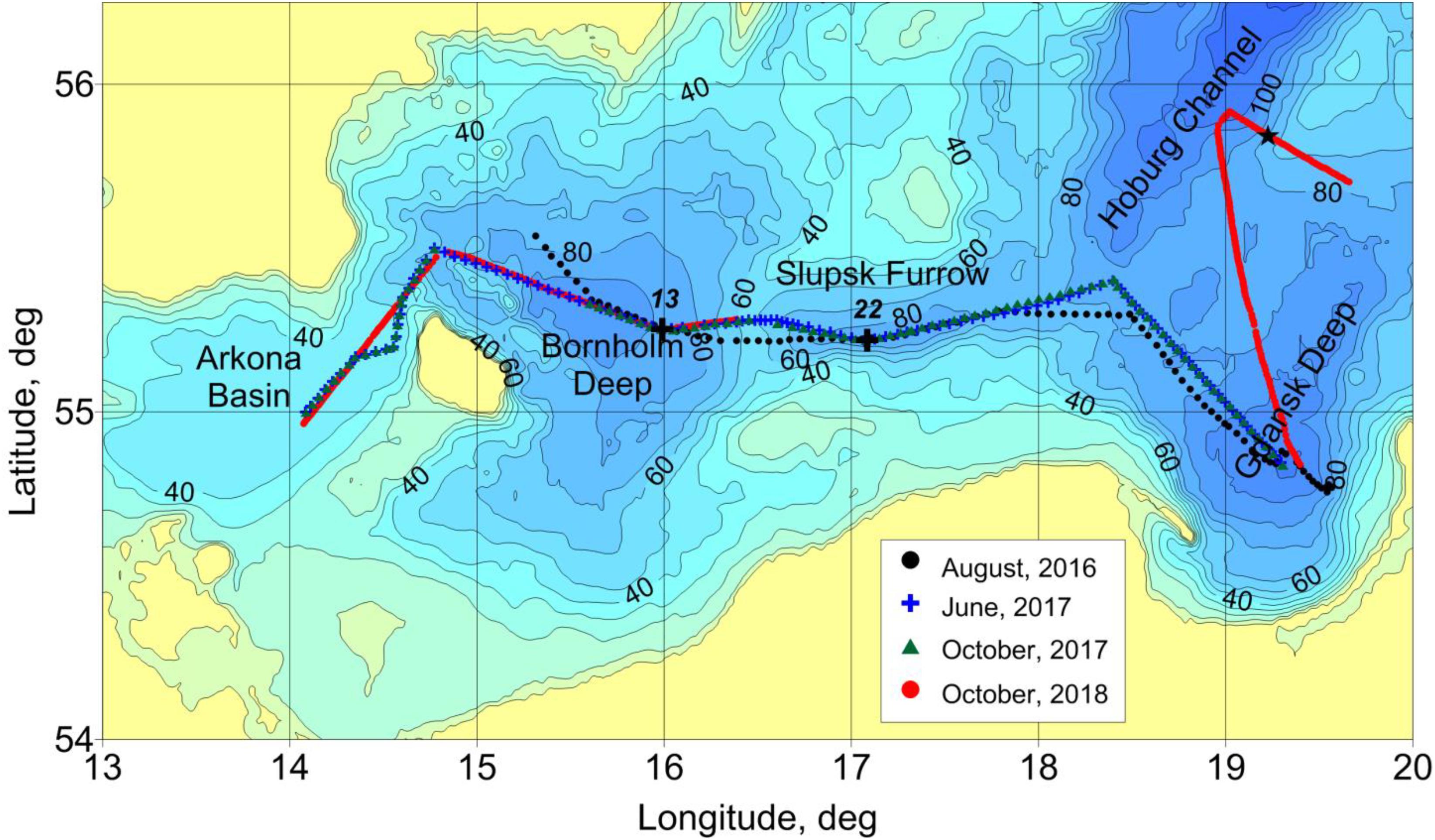
Figure 1. Location of the transects (color lines), the TCM deployment site (black star), and the IOW main monitoring stations, TF0213 and TF0222 (black crosses labeled as 13 and 22, respectively).

The field work on the transects in the 2016–2018 cruises was carried out taking into account the new requirements arising from the tasks of special monitoring. Before 2018, in order to obtain reliable information about the bottom parameters at all points of the extended transect, instead of towed scanning fish carrying the probe we had to return to measurements with the vessel on drift. Because of the ship’s stops every 2 miles, the mean speed of passage of the transect decreased twice relative to the towing speed with scanning. The modified measurement technique that we used in 2016 and 2017 was presented previously (Bełdowski et al., 2018a).

The probe Idronaut OS316+ was used in quasi-free fall mode. According to the manufacturer’s recommendations, the fall rate was 1 m/s and the probe reached the bottom and was kept on the seabed before recovery for at least 20 s, which made it possible to eliminate the inertial error of the estimates of the bottom parameters. Doing so, the most inert sensor—a polarographic oxygen sensor with the time constant of τ = 3 s—provided the correct result at the end of the stand. The proposed method of correction is explained in Figure 2, which shows one of the measurements by the OS316 + probe, performed in an area with a large gradient in the bottom layer. A fragment of a record of temperature T, salinity S, density σ_θ, and oxygen saturation O₂ signals as functions of time is presented. The black vertical line marks the moment of reaching the bottom. It can be seen that during the stay of the probe on the bottom, the signals T, S, and σ_θ practically did not change, whereas the O₂ signal regularly and expectedly changed, asymptotically approaching the value that differs from the initial one by 5% of saturation. Such a large error seems to be unacceptable, especially in the areas of steady hypoxia or oncoming hypoxia.

FIGURE 2

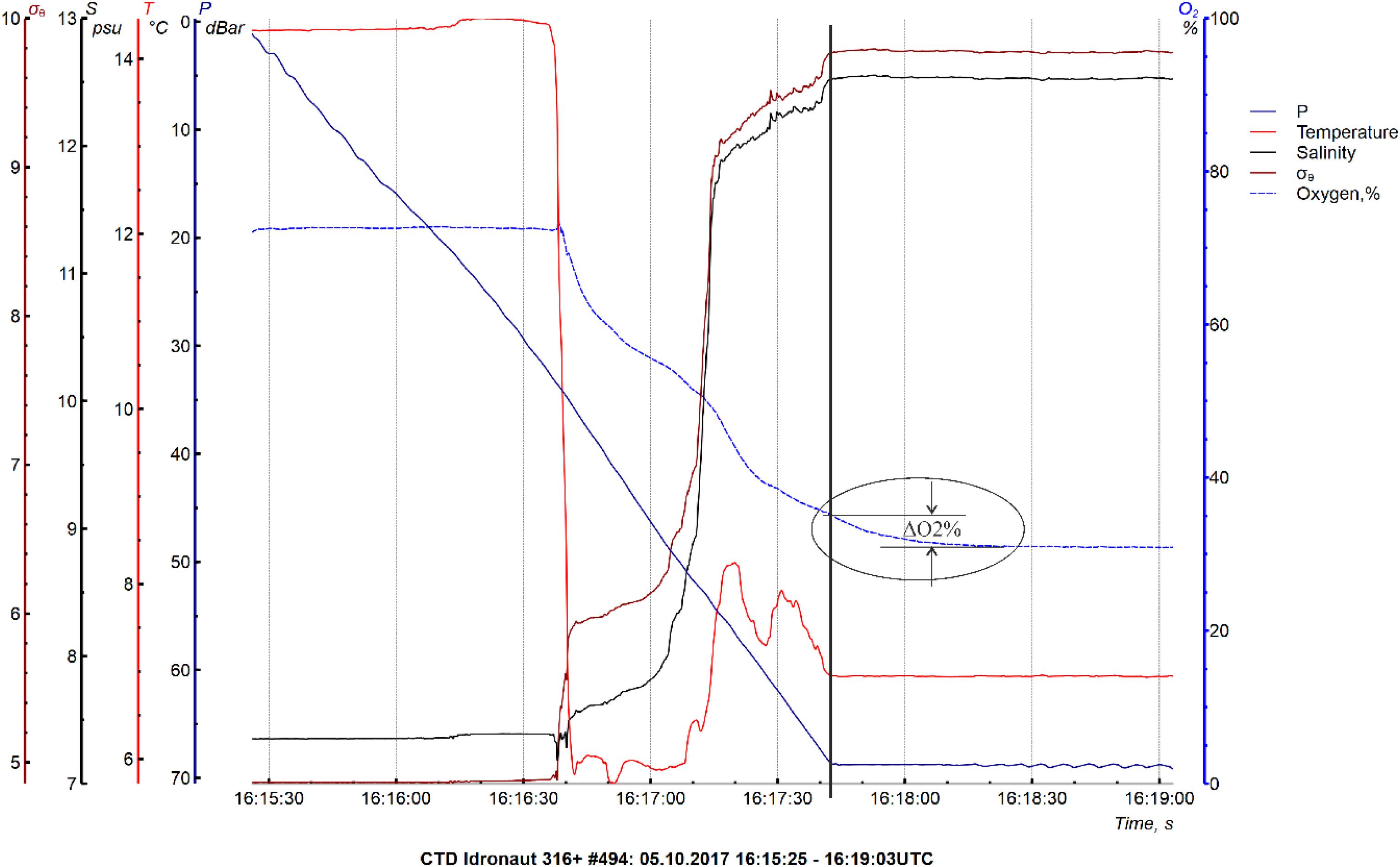
Figure 2. A record of temperature T (°C), salinity S (psu), density σ_θ and oxygen saturation O₂ (%) signals as functions of time during measurements at a drift station. The probe was kept on the ground for 1 min before recovery as can be seen from the pressure signal. The black vertical line marks the moment of reaching the bottom and the start of holding the probe at the bottom. The space between the horizontal lines placed in the ellipse shows the change ΔO₂ (%) in the oxygen saturation signal due to the oxygen sensor inertia. Note that the rest of the parameters, T and S, remained unchanged at this time.

Further, we managed to carry out the final modernization of the method of profiling from the moving ship and increased its speed to the initial value of 4–6 knots. According to the new method, a probe with a tether loosely coiled on the deck was released from the stern and began to sink down vertically, not perceiving the movement of the vessel. At the moment of termination of the free fall, the tether was tensioned, and the probe quickly rose to the surface. At this position, the recovery began. For recovery, a mechanism, which is a modified version of longline haulers designed for fishery, was used². It coils the tether on the deck instead of winding on the winch, and due to this allows repeating the next cast without delay due to preliminary preparation. Our mechanism provides a pulling force of about 50 kG, sufficient for recovery of the probe at a speed of about 1 m/s. For operation in this mode, the probe is placed between the load weighing about 5 kg and the float with a lifting force of about 2 kg, with the tether being fixed between the load and the probe, as shown in Figure 3. The load is chosen in such a way that the steady speed of fall is 1 m/s. When the bottom is reached, the probe, held by the float at a predetermined small distance from the bottom (40 cm), stops for a short time in the vertical position with the sensors directed downward (see Figure 3a). At the time of termination of the release, the tether is fixed on the deck, the outboard part is tensioned, and the onboard part is inserted in a hauler. Then, a recovery is implemented, ending when the probe approaches the stern. The bundle configuration during recovery is shown in Figure 3b. Unlike the towed probe, which rapidly moves with the travel speed at small distances from the bottom and with a high risk of scraping the bottom, the free-falling probe does not move in the horizontal direction from the moment of the beginning of free fall until the tether is fixed on the deck. Only when the probe takes off and is at a safe distance from the bottom does it perform horizontal movement. The loss of the probe with this sensing method is possible only due to the break of the tether, which is loaded with no more than 10% of the allowable tension.

FIGURE 3

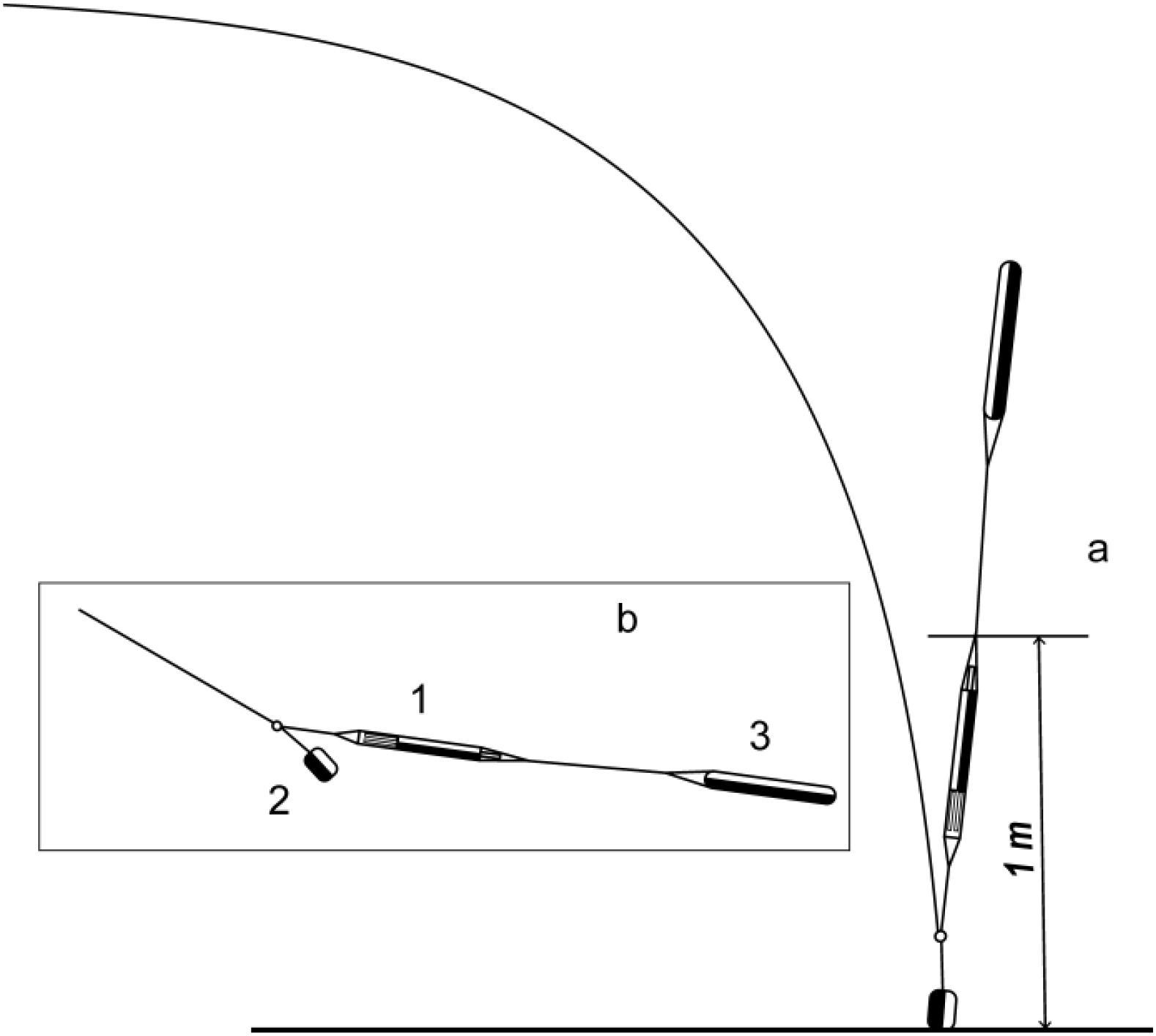
Figure 3. Arrangement of the profiling system, consisting of (1) CTD48Mc (Sea and Sun Technology), (2) load and (3) float, linked by pieces of rope. (a) Configuration when CTD reaches the bottom, (b) configuration during recovery.

The use of the new profiling technique does not obviate the need to correct the dynamic error of the inertial oxygen sensor. On the contrary, the problem is exacerbated because even short-term retention of the probe at the bottom, during which the rapid tether payout continues, results in a loss of time for the slow recovery of the released tether. The solution for this problem can only be a reduction of the inertia of the adopted oxygen sensor. In our last cruise we used the CTD48Mc probe from Sea & Sun Technology, equipped with a fast-response (∼1 s) optical sensor of dissolved oxygen saturation along with a standard set of CTD sensors with a sampling rate of about 10. Within this response time value remains an unintended pause, occurring after the command “stop” is executed on the winch, which lasts for at least 3–5 s. Therefore, working with CTD48Mc, we did not resort to a special delay, and the analysis of continuous records of signals confirmed the absence of an explicit dynamic error. The memory capacity of the probe was sufficient for several hours of continuous work.

The measurements using the new technique were carried out in various regions of the southern and central Baltic in the depth range from 45 to 120 m on a speed of about 5 knots with a frequency of about 8 cycles per hour, which corresponds to a spatial resolution of about 1 km. Approximately the same horizontal resolution is provided by towed scanning probes, but concerning the vertical resolution of the fine structure and reliability of the data in the bottom layer, obtained during contact with the bottom, the new method has an obvious advantage. It can also be noted that the developed measurement method does not require either powerful winches or cranes. Due to this, the method can be implemented on small vessels, which makes it promising for multiple uses.

Microstructure Measurements in the Bottom Layer

For additional measurements in the most interesting areas at the inflow pathway, a microstructure quasi-free (tethered) probe of our own design, “Baklan,” was used (Paka et al., 2010, Paka et al., 2013). The profiler was equipped with precision conductivity and temperature sensors manufactured at our special request by Idronaut S.r.l., a fast-response temperature sensor (type FP07) and an airfoil shear probe (type PNS06 from ISW). The sensors were sampled at 480 Hz with 16 bit resolution. Measurements in weakly turbulent regions showed that “Baklan” had a noise level of the order ε ≈ 10^-9 W/kg, which is sufficiently small to resolve dissipation rates in the turbulent boundary and shear layers. Sensors are protected from damage when they reach the bottom. This measure allows for probing at a very close distance from the bottom (∼10 cm).

Soundings are conducted at drift stations from the weatherboard or from the aft deck with the engine running if due to the weather conditions the vessel cannot be in free drift and is forced to move slowly upwind by bow trusters and a variable pitch propeller. The commonly practiced measurement technique, with the tether loosely slacked away from the deck after sinking the probe, is impossible under heavy drift since the tether lined up on the sea surface violates the vertical orientation of the probe, which is unacceptable for normal functioning of shear probes. Working from the aft deck when the vessel moves upwind is fraught with the risk of losing the probe, since strong wind gusts can force the vessel backward and the tether can get under the working propeller. When the vessel goes only forward, but not sufficiently slowly, then the same problem arises as during operation with a strong drift: the tether pulled out behind the vessel roll with the probe on its side and the turbulence sensor signal becomes noisy. To investigate the turbulence in any weather conditions, still allowing the vessel to work at sea, the construction of “Baklan” provides protection from the tether’s tension. Unlike other microstructure sounds (MSSs), “Baklan” stores a necessary length of the tether inside its body. During the fall, the tether freely leaves the magazine at the tail end of the probe and does not affect the movement. A capron cord has almost zero buoyancy in water; therefore, when the cord is pulled out, the mass of the sinking body does not change. The magazine holds up to 500 m of a thin (4 mm) cord, which makes it possible to use the probe anywhere in the Baltic Sea even in cases when the vessel moves away from the sensing point, with a speed exceeding the speed of the falling probe (60 cm/s) when using other probes is impossible or difficult.

Measurements of Current in the Bottom Layer

To study the spatiotemporal variability of currents in a thin bottom layer, autonomous instruments are necessary, which can be located at a minimum distance from the bottom in a sufficiently large number of points. Universal current meters, in particular acoustic profilers, are of little use for this purpose, because of the fundamental impossibility of measuring near the surface, which reflects an acoustic signal, and because the cost of multiple use is too high. Our choice fell on TCMs, the principle of operation that is based on measuring the inclination of the pendulum under the condition of equal forces of hydrodynamic pressure and buoyancy. We have developed our own device design, shown in Figure 4.

FIGURE 4

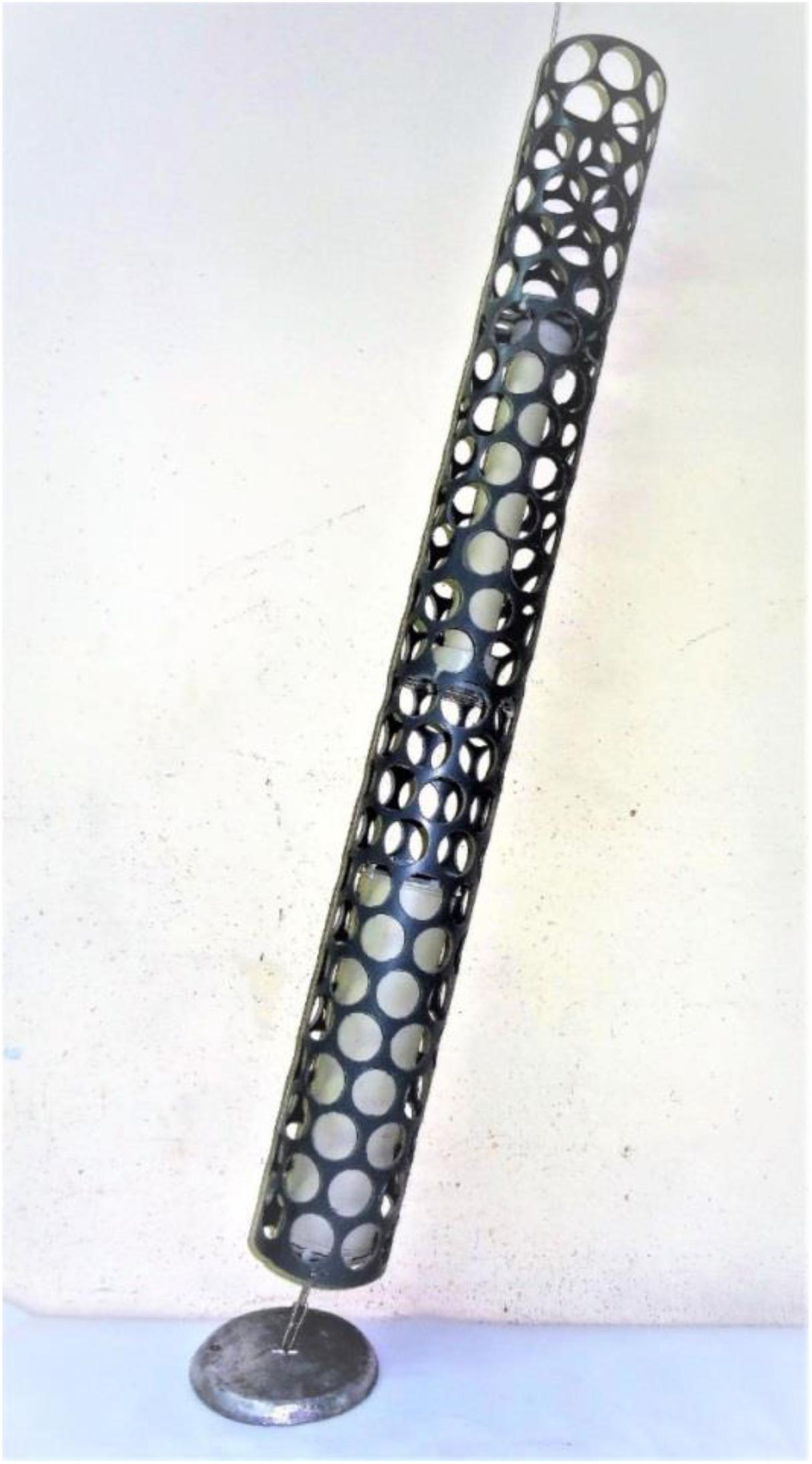
Figure 4. A photograph of the TCM. Its shape is formed by a cylindrical perforated plastic pipe. Inside there are an instrument and buoyancy modules, and the entire floating package is attached to a lead plate by a piece of chain.

The device can be manufactured in two versions—with positive or negative buoyancy. The second version is more complicated than the first one, but its sensitivity has a wider range and it can be used to measure strong currents, for example those occurring in the coastal zone. Figure 4 shows a TCM with positive buoyancy, designed to measure weak and moderately strong currents in the open sea, for which we were preparing. The body of the device has a cylindrical shape. The main disadvantage of the cylindrical shape is the formation of Kármán vortices during a cross-flow and, as a result, the occurrence of auto-oscillations, but this refers to a smooth cylinder. A hard cylindrical perforated shroud is flown around without the formation of coherent vortices and does not oscillate. We utilized this property.

The shroud is made of a thin-walled plastic pipe with a diameter of 110 mm, a length of 1 m, and is evenly perforated with a perforation factor of about 50%, as can be seen in Figure 4. The dimensions of the shroud are chosen taking into account the dimensions of the instrument module and the thickness of the layer under study. A watertight module with electronics is placed in the lower part of the shroud at a minimum distance from the pivot point so that the accelerometer that measures the angle of inclination weakly reacts to linear accelerations due to rapid transient responses. In the same module, there are an electronic compass, which determines the direction of tilt of the cylinder, an electronic clock and other elements that ensure continuous autonomous operation of the device with the possibility of programming the ratio of recording time and pause.

A precision watch was provided with the monthly accuracy of 10 s, which in the first approximation can be considered sufficient to perform synchronous measurements in a large number of points (in perspective). The buoyancy of the instrument module is close to neutral. To increase the buoyancy, a cylindrical float is placed in the upper part of the shroud (see Figure 4). By shifting it along the shroud, it is possible to change the moment of the buoyancy force, adjusting the sensitivity of the device. Sensitivity can be increased as long as acceptable stability of the signal corresponding to zero flow velocity is maintained. Studying the behavior of the device in standing water, it was determined that the lower threshold of measured speeds can be considered 2 cm/s with a relative accuracy of 25%. The full range of measured speeds at a setting for maximum sensitivity is 2–30 cm/s, with a maximum speed measurement error of about 3%. With a coarser adjustment of the sensitivity, the measuring range remains the same. Therefore, the increase of the maximum measured speed up to 1 m/s and more comes on the expense of the accuracy of measuring of weak currents.

We managed to achieve satisfactory quality of our products and calibrated them in the towing tank just before the last cruise. Field tests of new equipment were carried out in an area located on the eastern slope of the Hoburg Channel, along which saltwater flows into the Gotland Deep. Saltwater can come to the Hoburg Channel either directly from the Słupsk Furrow or in a roundabout way through the Gulf of Gdansk, and the choice of the route is probably controlled by the wind field over the water area. On a fragment of the bathymetric map (Gelumbauskaite et al., 1999) presented in Figure 5, the arrow shows a small gully along which saltwater can move from the Gulf of Gdansk in the direction of the arrow. In particular, this site was chosen for testing of TCMs. A group of 10 instruments were tested, and they were identically configured to measure currents with speeds of up to 60 cm/s (the float was placed in the upper part of the shroud, as can be seen in Figure 4). All instruments were deployed as a compact group so that they would be at equal conditions and show similar results. The tests were successful. All ten 5-day records turned out to be similar in terms of both slow and fast changes in flow. Based on this, we can use the data to describe the characteristics of the bottom current in the selected area (see section “Near-Bottom Currents”).

FIGURE 5

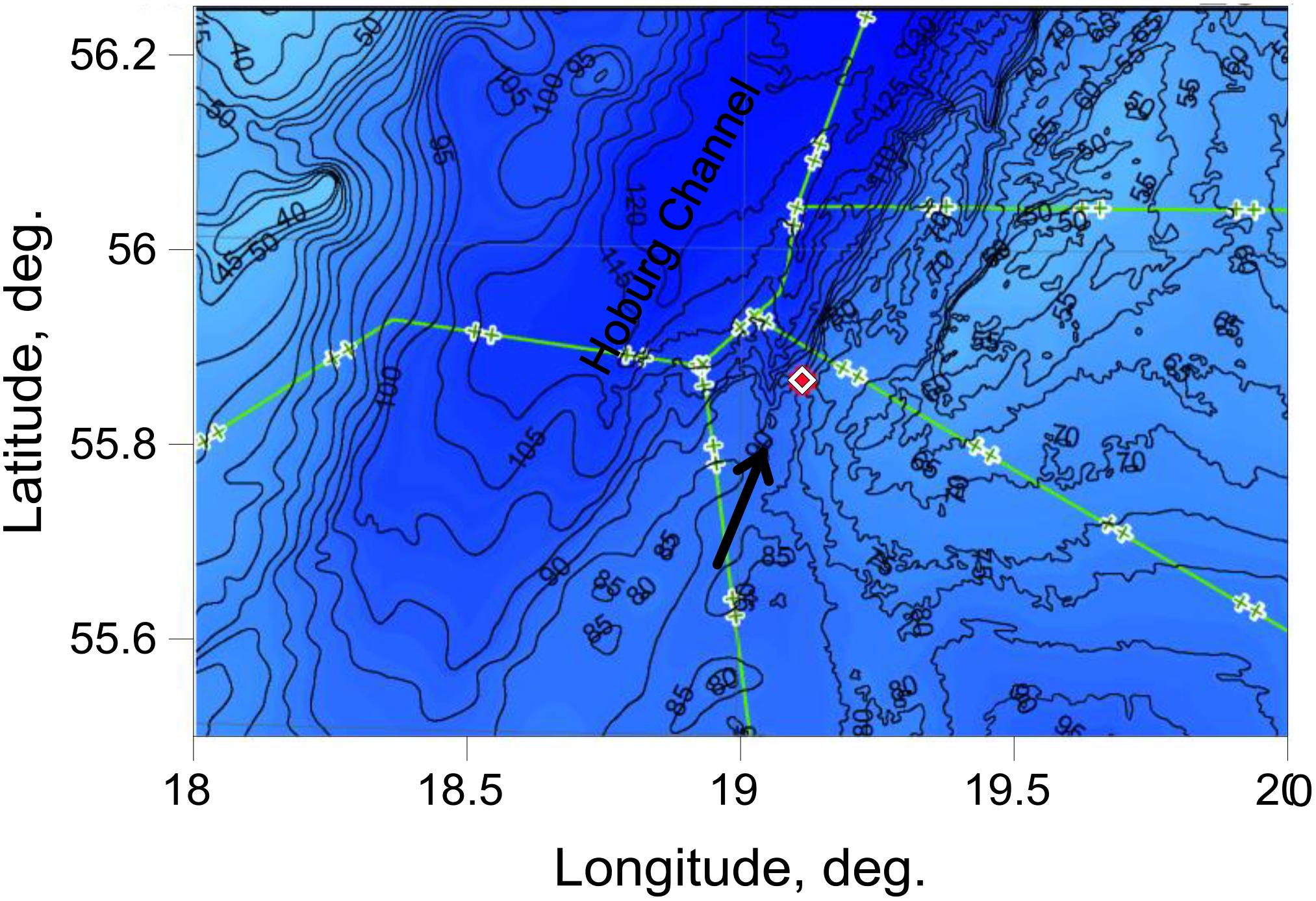
Figure 5. Bottom relief and position of TCMs’ group (diamond) at the test area. Lines mark boundaries of Exclusive Economic Zones of the Baltic States. Arrow points to the gully.

Results

Results of Measurements on the Extended Transects

The transects demonstrate the water structure from the surface to the bottom, but changes in the surface’s mixed and cold intermediate layers (CIL) are not a matter for analysis within the frame of our task. Each of these layers was formed in the process of the heat and momentum exchange with the atmosphere and is practically insensitive to the inflows, so they are not of particular interest for analyzing changes of water structure below the permanent halocline. The only parameter that depends on the intensity of the saltwater inflows is the depth and topography of the lower boundary of the CIL, since it corresponds to the upper boundary of the halocline. The halocline depth in the Bornholm Deep relative to the Słupsk Sill depth characterizes the ability of saltwater to spread eastward in the form of near-bottom gravity current.

Except for the periods of sufficiently powerful inflows that are able to ventilate the deepest layer of the Bornholm and Gdansk basins, the saltwater layer in the southern Baltic Sea can be divided into two parts: the upper, variable part corresponding to the interleaving zone of moderate and weak inflows, and the lower, conservative part containing water with maximum salinity and density where the moderate and weak inflows do not penetrate. If the period of lack of sufficiently powerful inflows lasts for a long time, then stagnation develops in the lower layer. Additionally, there are rare events of the most powerful inflows called the Major Baltic Inflows (MBIs) that can ventilate, apart from the Bornholm and Gdansk deeps, the deepest Baltic basins such as the Gotland Deep [see, e.g., Matthäus and Franck (1992)]. The last MBI took place in December 2014. The recent analysis of MBI statistics showed that until today, climate change has no obvious impact on the MBI-related oxygen supply to the central Baltic Sea, and the increased eutrophication during the last century is most probably responsible for temporal and spatial spreading of suboxic and anoxic conditions in the deep layer of the Baltic Sea (Mohrholz, 2018).

The first survey (Figure 6) was carried out at a time when the surplus of saltwater in the Bornholm Basin due to MBI 14 overflowed the Słupsk Sill, as a result of which the halocline depth in the Bornholm Basin decreased to the depth of the Słupsk Sill; the same happened beyond the Słupsk Sill in the Słupsk Furrow, where the halocline depth decreased to that at the exit from the Słupsk Furrow. In the Gdansk Deep, the halocline level was observed even deeper. In the Bornholm and Gdansk Deeps, the oxygen content dropped to almost zero. At the same time, in the Słupsk Furrow, through which the oxic water passes from the intermediate layers of the Bornholm Basin, the oxygen saturation was 30%, but, as we see, this water did not reach the bottom of the Gdansk Deep. There were no signs of active intra-basin dynamics in any of the basins. At the Słupsk Sill, the salinity contours of more than 9 psu had a gap, which can be considered as an indication of the absence of a significant saltwater overflow. However, water with salinity of about 14 psu was very close to the top of the Sill, which indicates a high probability of resumption of saltwater overflow, both as a result of a new, even weak, inflow into the Bornholm Basin, or as a result of fluctuations of the halocline level in the vicinity of the Słupsk Sill due to some dynamical reasons.

FIGURE 6

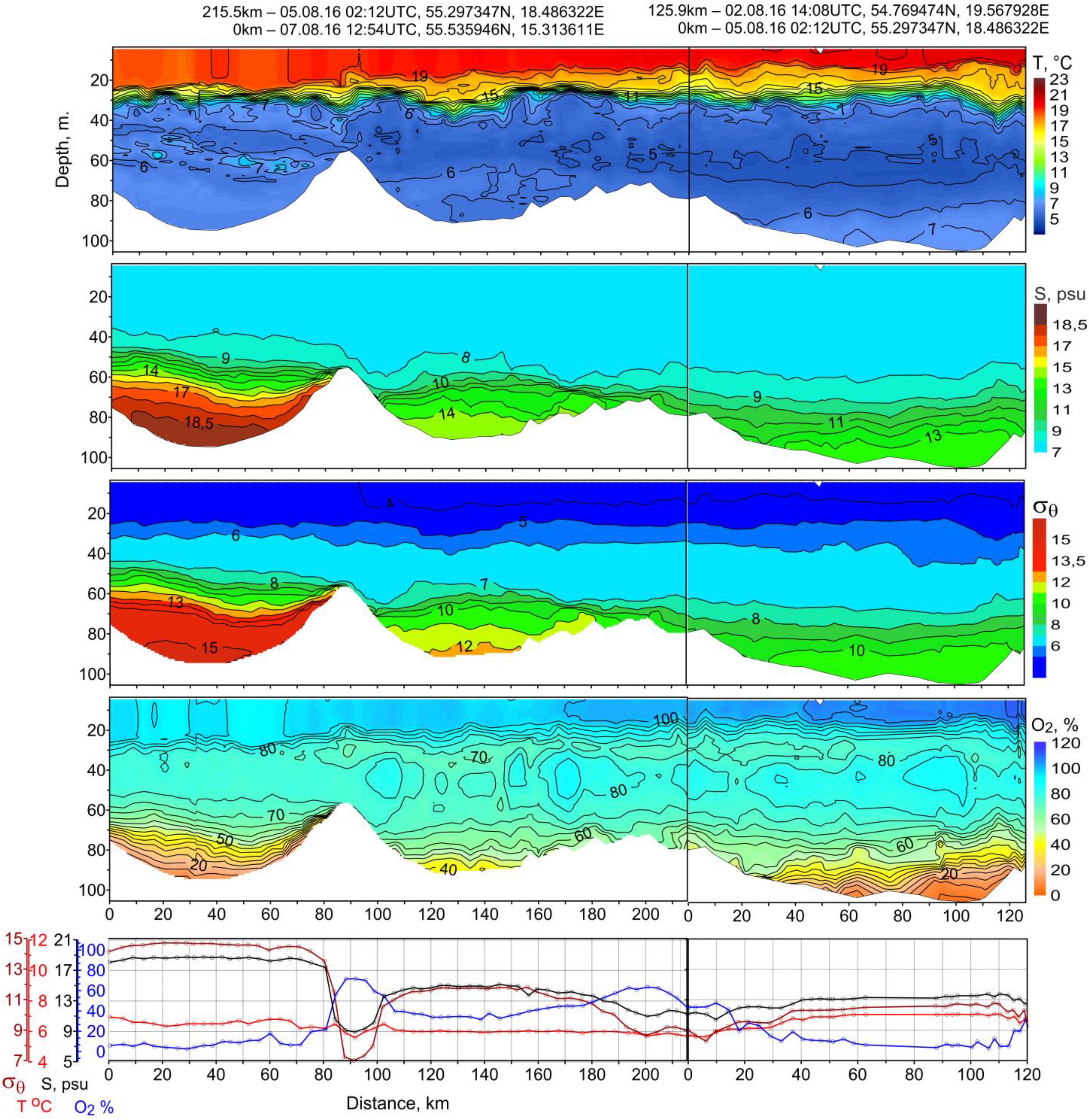
Figure 6. Distributions of temperature T (°C), salinity S (psu), density σ_θ, and oxygen saturation O₂ (%) in the southern Baltic for the 1st survey (August 2016); bottom panels demonstrate graphs of the same parameters in the bottom layer.

The second survey (Figure 7), carried out 10 months after the first one, showed a significant reduction in the volume of the saltiest/densest water, with a salinity of above 17 psu in the bottom layer of the Bornholm Deep and a simultaneous decrease of the maximum salinity and density, but in the upper saltwater layer the volume of less saline water (<17 psu) increased so much that the halocline level appeared to be elevated several meters above the Słupsk Sill depth. The conclusion is that during the preceding 10 months, there was no inflow of water capable of reaching the bottom, but there were likely some weak or moderate inflows which formed the interleaving and led to a rise of the halocline depth. The difference in halocline levels on both sides of the Słupsk Sill, determined conventionally by the isohaline of 9 psu, was 15 m, which indicates the formation of a gravity current above the eastern slope of the sill. This overflowing water was well oxygenated (60% of saturation), and in the Słupsk Furrow the saturation never decreased below 20%. But the activity of water exchange through the Słupsk Sill did not affect the stagnation in the Bornholm bottom layer, where the anoxic zone at the bottom occupied 80 km along the line of the transect between the isobaths 72 and 83 m. As for the Gdansk Deep, the oxygen content there even slightly increased. Apparently, the bottom layer here was partially ventilated by oxic water flowing through the Słupsk Furrow.

FIGURE 7

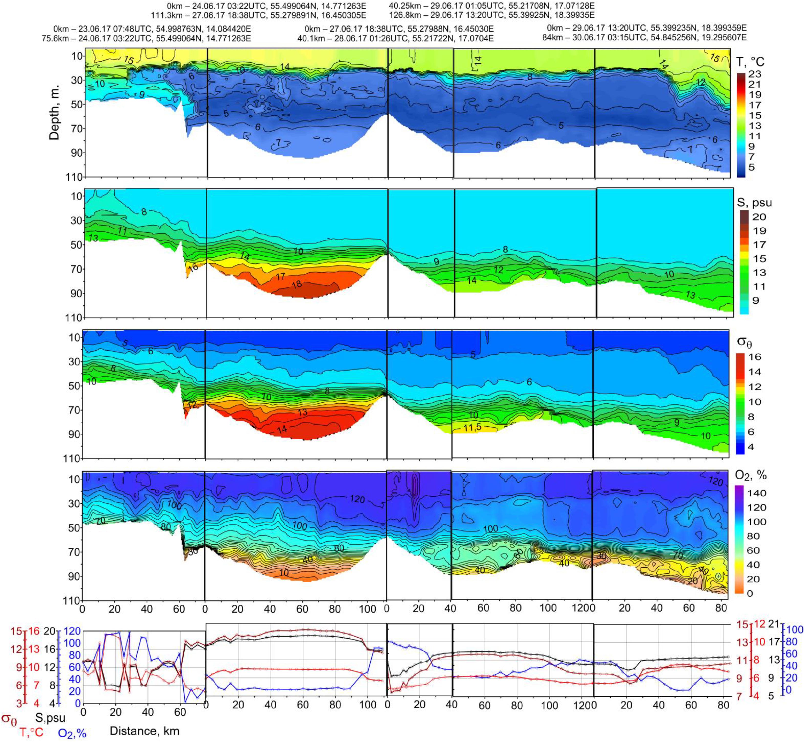
Figure 7. Distributions of temperature T (°C), salinity S (psu), density σ_θ, and oxygen saturation O₂ (%) in the southern Baltic for the 2nd survey (June–July 2017); bottom panels demonstrate graphs of the same parameters in the bottom layer.

The third survey (Figure 8) was made 4 months after the second. In this short time, the topography of the halocline near the Słupsk Sill was radically changed. The isohaline of 9 psu denoting the upper border of the halocline was found at a depth of 50 m, or 7 m above the Słupsk Sill depth, but the high level of the halocline was also observed just beyond the sill, which is not typical for this area and impedes the formation of a gravity current beyond the Słupsk Sill. One may suppose that the saltwater overflow stopped due to a surge of saline water toward the Sill from the middle of the Słupsk Furrow, which was most likely a consequence of the synoptic processes in the Southern Baltic (Krauss and Brügge, 1991). As for the maximum salinity in the bottom layer of the Bornholm Deep, Słupsk Furrow, and Gdansk Deep, it continued decreasing, as can be seen from the data presented in Table 1.

FIGURE 8

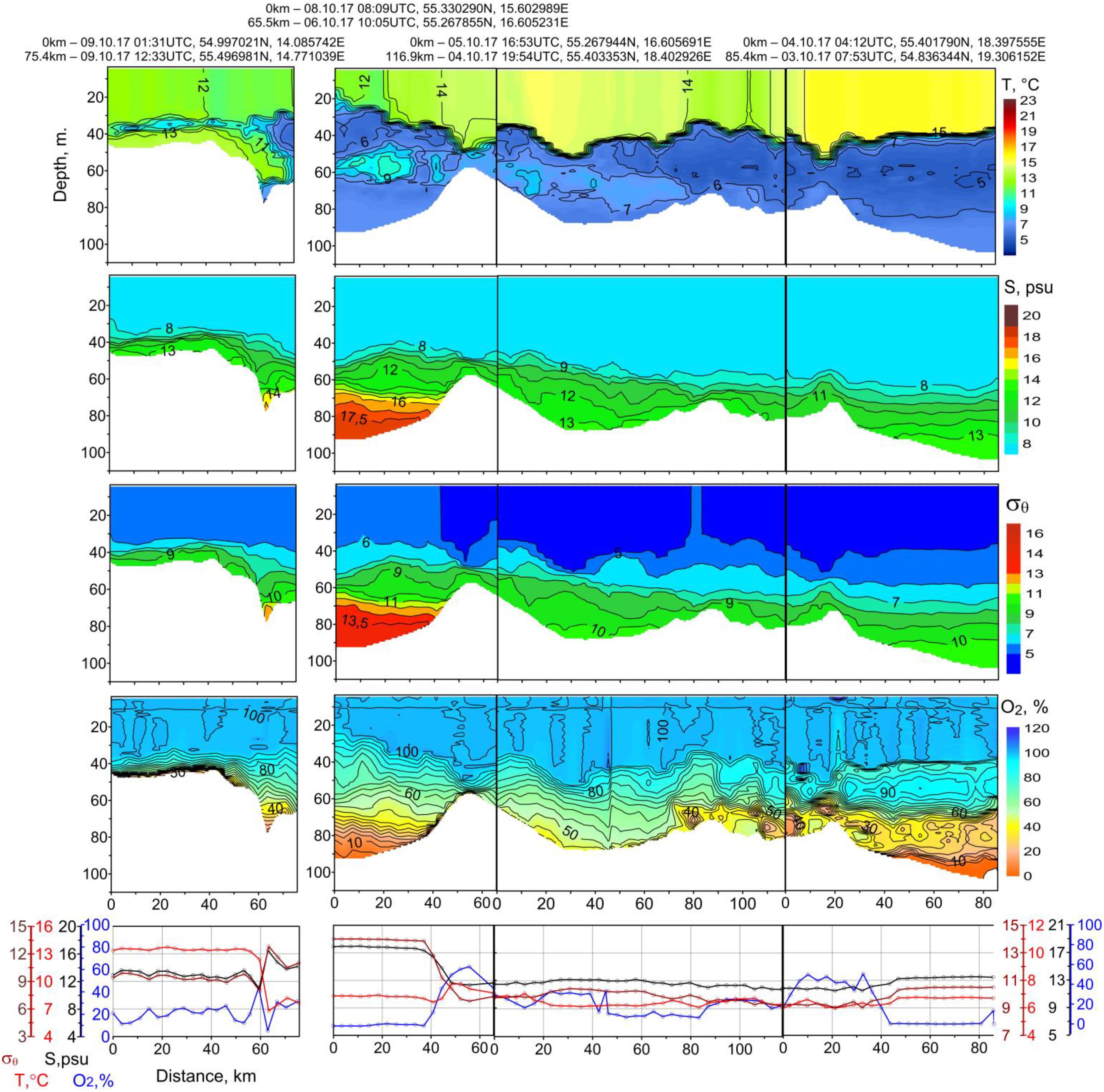
Figure 8. Distributions of temperature T (°C), salinity S (psu), density σ_θ, and oxygen saturation O₂ (%) in the southern Baltic for the 3rd survey (October 2017); bottom panels demonstrate graphs of the same parameters in the bottom layer.

TABLE 1

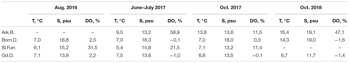
Table 1. Maximum bottom temperature, salinity and minimum dissolved oxygen (DO) saturation at the transects through the southern Baltic basins.

The fourth survey (Figure 9), carried out 1 year after the third one, showed radical changes of the water structure in the Arkona and Bornholm Basins. Nothing like that happened in the Gdansk Deep. In the Słupsk Furrow and on the Słupsk Sill, measurements were not taken due to the lack of permission to work in Polish waters. Evidently, an inflow occurred, manifested in the renewal of the bottom waters in the Bornholm Deep. Together with the salty, dense and warm water, a large amount of oxygen was supplied (see Table 1). Judging by the horizontal heterogeneity of the density field, the inflow water has not yet found its stable position in the deep. This is evidenced by the signs of spreading of relatively warm, maximum saline/dense and sufficiently oxic water from the core, located in the central part of the deep with a slight shift to the east with the upper boundary conventionally determined by the 18 psu contour, at a depth of 80 m. In the process of spreading, a layer stretching to the west at a distance of about 20 km was formed so thin that it could only be detected by the new method of measuring the bottom parameters. In the western part of the deep in the near-slope region, another large new water pool was observed with T = 13°C and S = 18 psu, the upper boundary of which was situated even higher—at a depth of 68 m. From this water body, a thin layer of salty/dense water—even richer in oxygen than in the central intrusion—spread to the east descending to greater depths. In addition, large intrusions with a slightly lower salinity of 14.5–15.5 psu reached a depth of 55–60 m, corresponding to the depth of the Słupsk Sill. These intrusions, as well as the bottom ones, also have a temperature of about 13°C, which is higher than the temperature of the surrounding water by 3°C, undoubtedly indicating its recent arrival from the Arkona Basin, where the entire water column, with the exception of a thin layer at the halocline border, has a temperature of about 12.5–13.5°Ñ.

FIGURE 9

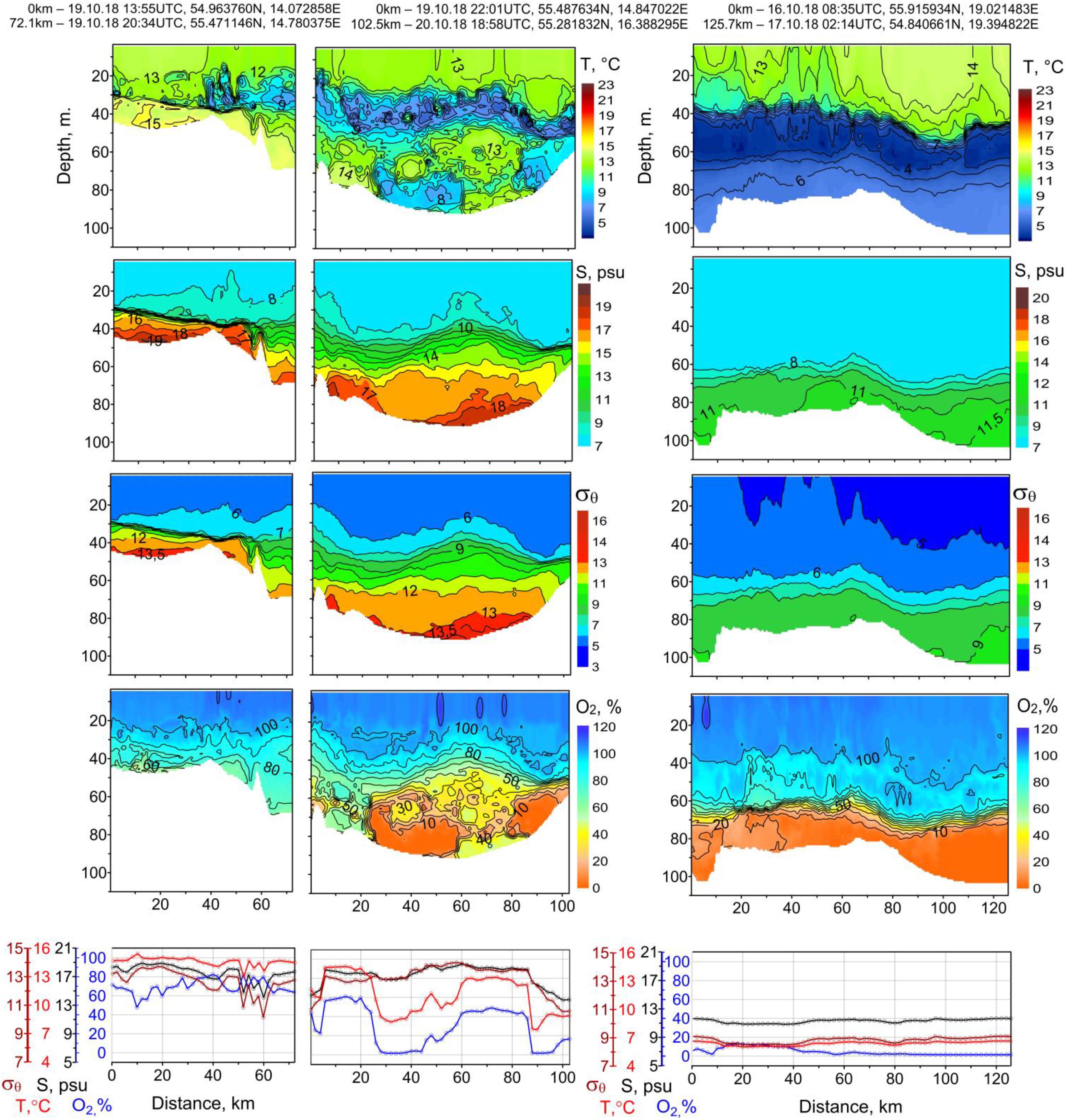
Figure 9. Distributions of temperature T (°C), salinity S (psu), density σ_θ, and oxygen saturation O₂ (%) in the southern Baltic for the 4th survey (October 2018); bottom panels demonstrate graphs of the same parameters in the bottom layer.

Warm water intrusions in the bottom and intermediate layers below the permanent halocline in the Bornholm Deep (Figure 9) indicate a strong baroclinic inflow event that took place in autumn 2018 (Volker Mohrholz, personal communication). Note that in the past, the highest ever recorded temperature of 13.9°C in the halocline of the Bornholm Basin was measured in October 2002 after an exceptionally warm summer inflow event (Mohrholz et al., 2006). In October 2018, this temperature record was exceeded by 0.4°C: the maximum temperature in the Bornholm Deep halocline rose to 14.3°C.

The maximum values of salinity and minimum values of dissolved oxygen (DO) saturation at the bottom in the Bornholm Deep and Słupsk Furrow recorded at the extended transects (Table 1) are close to the IOW monitoring data obtained using the standard method at stations TF0213 and TF0222 (see Figure 1), respectively³. Some discrepancies can be explained by the fact that our data were selected from the transects, while the IOW data were obtained at single locations, and the main monitoring station in the Bornholm Deep (TF0213) was located not at the maximum depth of the basin (approximately 95 m) but at a depth of 88 m, where the bottom layer parameters could not reach their limits. Note that some of the minimum values of DO measured on the extended transects in the bottom layer of the Bornholm and Gdansk deeps are negative (see Table 1). We consider the negative DO values as an indicator of the presence of hydrogen sulfide, not as an error of calibrating the oxygen sensor. Our conclusion is qualitative, because we did not make a special calibration of the sensor with the purpose of quantitative determination of hydrogen sulfide content.

To provide more adequate comparison of our data with the IOW monitoring measurements of the oceanographic parameters at the bottom at stations TF0213 and TF0222, we chose values of temperature, salinity, and oxygen recorded at the same depth and as close as possible to the location and time allowed by the transects available (Table 2). Note that Table 2 does not contain the comparison for the October 2018 transect performed after the early Autumn 2018 baroclinic inflow event because the corresponding data of the November 2018 IOW monitoring cruise are not yet available at https://www.io-warnemuende.de/cruise-reports.html. According to Table 2, the oceanographic parameters measured in the near-bottom layer by the standard method in the IOW monitoring cruises correspond well to the IO RAS data obtained at the extended transects performed using the innovative measurement technique: the mean/standard deviation of the difference between the IO RAS and IOW data are -0.16/0.53°C, -0.17/0.38 psu, and -0.28/6.18% for temperature, salinity, and oxygen saturation, respectively. Since the time discrepancy between the IOW and IO RAS measurements was as large as 2 months, such a small discrepancy in the measured oceanographic parameters seems quite acceptable.

TABLE 2

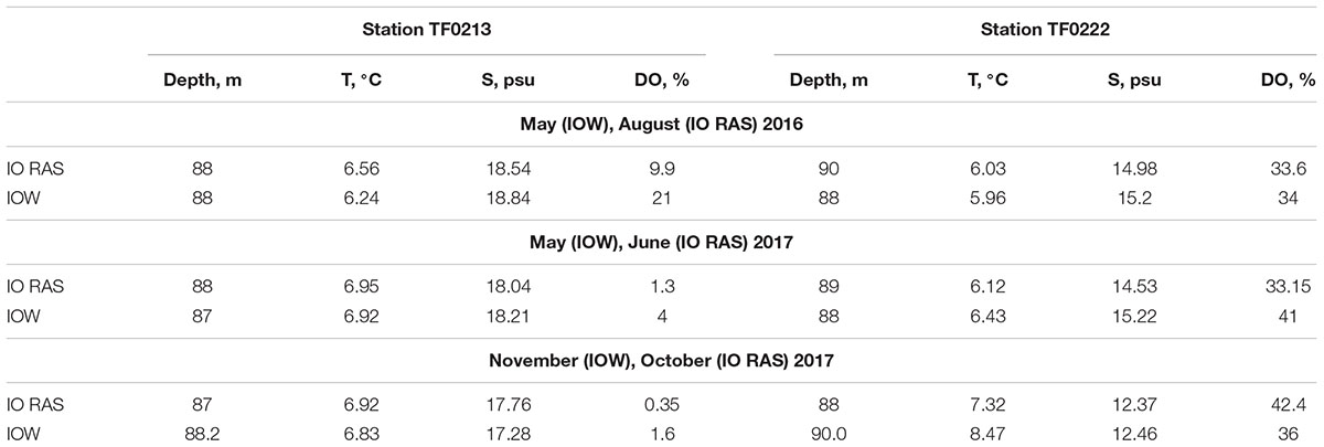
Table 2. Comparison of the bottom oceanographic parameters at the IOW monitoring stations TF0213 and TF0222 with the corresponding data extracted from the IO RAS extended transects.

Results of Microstructure Measurements

During the campaign, the microstructure measurements were carried out mostly in cases when in the water structure there were signs of a strong gravity current with a developed turbulence. On CTD transects, segments of high probability of turbulent motion in the bottom layer were distinguished as thin layers with increased salinity, located above the sloping bottom. It is just the way the gravitational current manifests in the thermohaline structure. A targeted search for turbulent bottom currents was performed over the Słupsk Sill, where this property was predicted (Piechura et al., 1997) and found by direct measurements, as reported by Mohrholz and Heene (2018) at the 2nd Baltic Earth Conference in Helsingor, 2018. Favorable conditions were observed in July–August 2017. In the next survey in October 2017 at the same site, there were no signs of a gravity current in the bottom layer, but we decided to investigate this situation anyway. This allowed us to evaluate and compare turbulence for a situation, different from the strong eastward overflow, when nevertheless a weaker flow occurs, and its interaction with the obstacle can generate nonstationary turbulence with poorly studied properties.

Examples of microstructure measurements performed in July and October 2017 are presented in Figures 10, 11. All data including the pressure signal are drawn as time functions, and the time is replaced by number counts. To show a background water structure, the microstructure plots are accompanied by the temperature, salinity and density plots. A dashed line marks the end of the probe’s motion when it reaches the seabed, and at this moment the pressure signal becomes constant, while any changes of other signals do not carry any information.

FIGURE 10

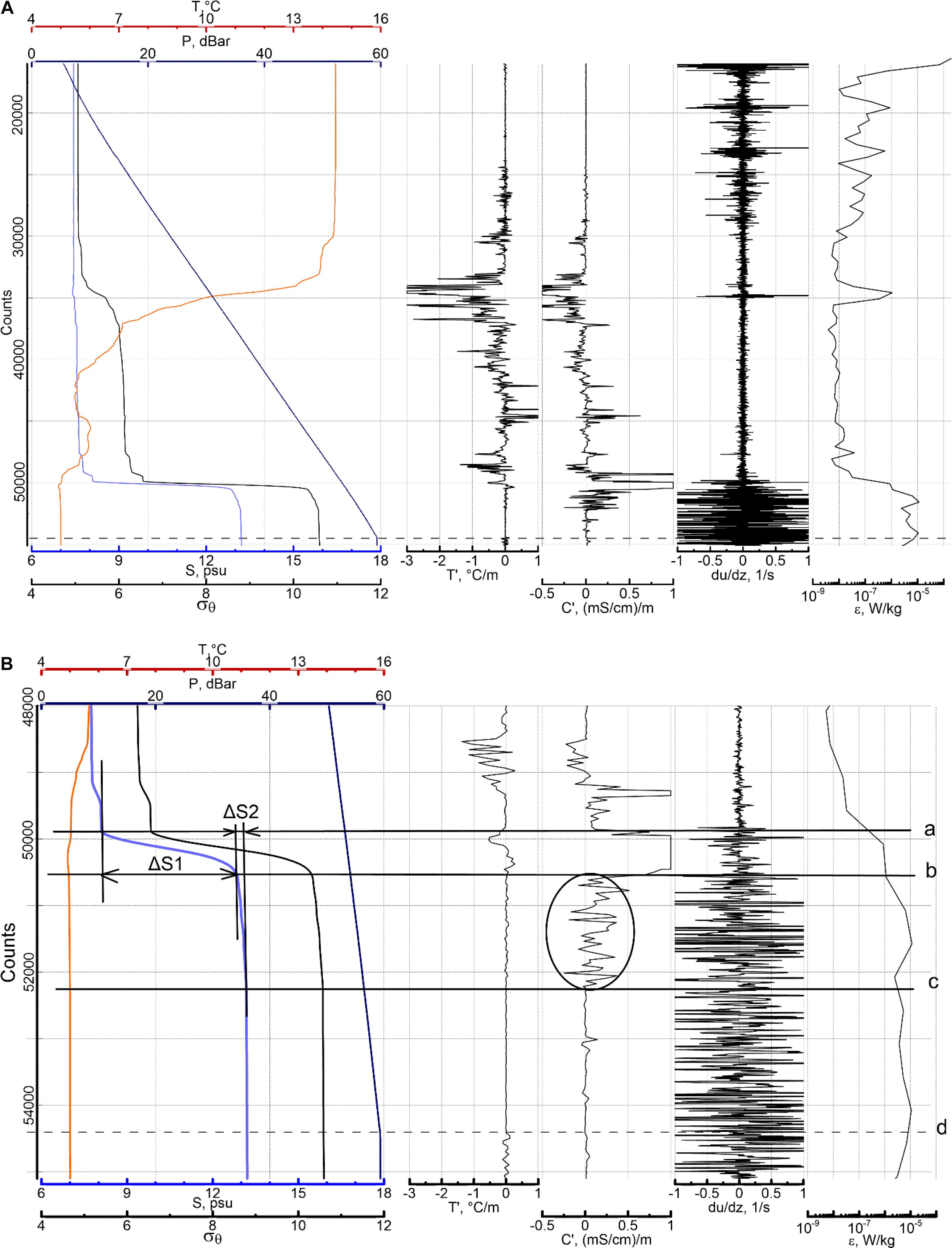
Figure 10. (A) Example of turbulent bottom layer on the Słupsk Sill, the profile was registered on 02.07.2017, 19:40 at the following position: 55° 13.167′N, 16° 33.423′E. A westerly wind of 5–15 m/s prevailed. On the left panel: temperature T, °C; salinity S, psu; density σ_θ, pressure P, dBar. On the next panels from left to right: microstructure of temperature T′, °C/m and conductivity C′, (mSim/cm)/m; shear velocity fluctuations du/dz, 1/s; dissipation rate ε, W/kg. Dashed line marks the moment when the probe reaches the seabed and the pressure signal becomes constant. (B) Zoomed fragment of the profile shown in (A) presenting the fine- and micro- structures of the salt/dense bottom layer. Horizontal solid lines show upper bounds of (a) high gradient sheet, (b) moderate gradient sublayer (entrainment layer), (c) homogeneous sublayer; dashed line (d) marks the end of profiling. Ellipse marks a segment of developed conductivity microstructure. Crossing of the salinity plot with vertical lines show where salinity increments ΔS1 = 4.68 psu and ΔS2 = 0.29 psu were evaluated.

FIGURE 11

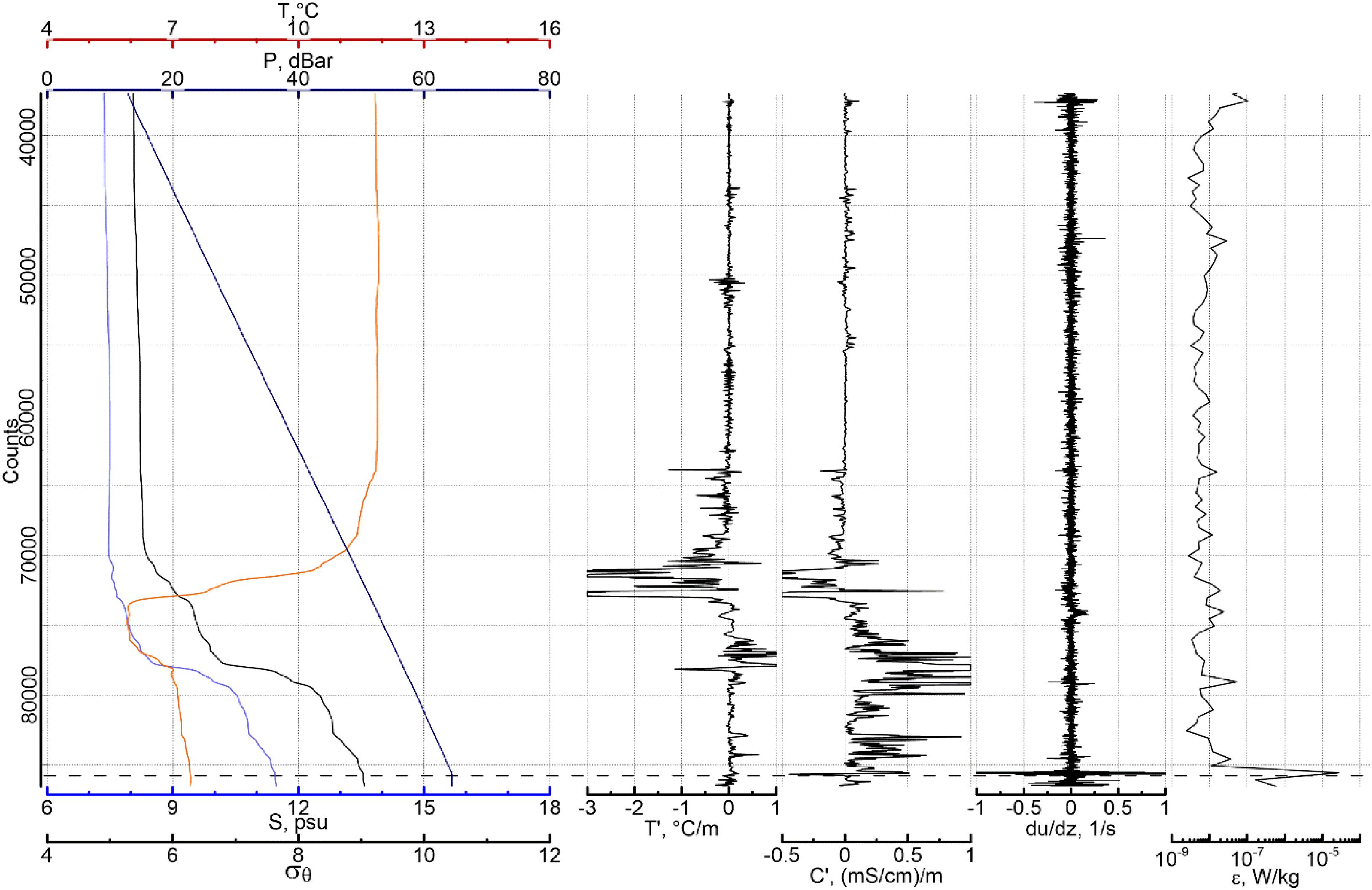
Figure 11. Examples of non-turbulent bottom layer on the Słupsk Sill, the profile was registered on 18.10.2017, 14:03 at a position 55° 17.999′N, 16° 31.350′E. A westerly wind of 5–10 m/s prevailed. The presented variables are the same as in Figure 10A.

The vertical microstructure is closely related to the background stratification, and the upper quasi homogeneous layer can be distinguished. Within the upper mixed layer, which is under the direct influence of wind and surface waves, turbulence decreases with depth from a maximum value of ε∼10^-4–ε∼10^-8 W/kg, approaching the thermocline at a close but definite distance with a value of ε ∼ 10^-7 W/kg (Figure 10A). The vessel’s weather station during the experiment recorded a wind of 10–15 m/s from W-NW; its stress was not enough to perform the mixing to the depth of the main thermocline, which was apparently formed with a stronger wind. The distribution of turbulence with depth within the mixed layer is uneven. It is possible to allocate two sublayers, analyzing the microstructure not only for the shear velocity du/dz, but also for temperature T′ and conductivity C′, the last is a function of temperature fluctuations because the salinity gradient is weak. The surface sublayer is characterized by maximum dissipation rate and by completely smooth scalar fields. In the next sublayer, there are a noticeable scalar microstructure and decrease of dissipation rate. It can be noted that this feature corresponds to the erosion of a thermocline under the influence of turbulent entrainment.

The layer situated between the seasonal thermocline and the permanent halocline is characterized by a well-developed microstructure of scalar fields. The core of this layer is the cold intermediate layer (CIL) with a temperature of 5.5°C at depths of 40–45 m. Being in permanent interaction with overlaying and underlying layers, CIL is subjected to continuous erosion, reducing its thickness. The distribution of density in the upper part of the intermediate layer is determined by temperature, while in the bottom part is determined by salinity. The density gradient is not as great as in the main halocline and, hence, it is not a big hindrance to stirring. As a result of such stirring, a scalar microstructure is formed, the intensity of which depends on the temperature and salinity gradients in the presence of a weak shear of the velocity originated by the independent motion of the upper and bottom layers. However, the level of turbulence here is small (ε ≈ 10^-8 W/kg). Short sharp impulse on the plots of shear signal du/dz and dissipation rate ε at the depth of the thermocline is undoubtedly an artifact, the result of collision with the extraneous object.

Similarity of the microstructure of the temperature and conductivity fields is disturbed only near the halocline, which indicates that from this depth the determining factor becomes the distribution of salinity.

The bottom layer is easily distinguished by increased salinity and density. In July 2017, there was a 6 m thick bottom layer with a salinity/density increasing from 8.16 psu/6.55 σ_θ at the top of the layer to 13.16 psu/10.57 σ_θ at the bottom, with the temperature only slightly changed. The distribution of all parameters within the saltwater layer is not as homogeneous as what might have been expected due to the fact that the dissipation rate here reaches ε = 10^-5 W/kg. To show some peculiar properties of the turbulent bottom layer, let us consider its zoom in Figure 10B. There are three horizontal solid lines which mark the following: (a) an upper boundary of high gradient sheet that is 0.9 m thick and with a salinity increment of ΔS1 = 4.68 psu; (b) a moderate gradient sublayer, or an entrainment layer that is 2.5 m thick—the salinity increment here is ΔS2 = 0.29 psu; (c) a homogeneous sublayer that is 2.8 m thick with zero salinity increment. Dashed line (d) marks the end of profiling. The mentioned sheet and sublayers have different microstructure. Within the highest gradient sheet, the microstructure is not expected. The entrainment sublayer must have the microstructure due to entrained water of lesser salinity, and it is clearly seen in the conductivity signal. Temperature pulsations are insignificant, as the temperature in the bottom layer changes in narrow limits.

In October 2017 the bottom layer with increased salinity (up to 11.4 psu) and density (up to 9.0 σ_θ) also existed, but its properties changed as is clearly seen in Figure 11. There was no sharp interface. Within the bottom boundary layer, the previously mentioned homogeneity of the fields T, S, and σ_θ disappeared, while the microstructure of scalar fields appeared. This occurred due to the increasing of the density gradient and weakening of the turbulence; the dissipation rate decreased to the value of 10^-8 W/kg, which was typical for the main part of the water column below the upper mixed layer.

Thus, we obtained quantitative data characterizing microstructure properties for two situations which could be considered as typical for the Słupsk Sill when the period of time passed from an MBI exceeds 1 year. The first situations correspond to the moderate activity of salt water overflow, when the elevation of the halocline in the Bornholm Deep with respect to the Słupsk Sill exists but is not very high, while the halocline in the Słupsk Furrow is situated deeper than the depth of the sill (see Figure 7). The second situation corresponds to interruption of the continuous overflow, when the difference of halocline depths at the west and east edges of the Słupsk Sill disappears (Figure 8). This occurs due to some kind of synoptic reasons, which are not extraordinary, which is why we consider this situation as also typical for the Słupsk Sill area.

Data of microstructure measurements performed in July 2017 revealed a high turbulence dissipation spot immediately beyond the sill in the near-bottom layer filled with eastward spreading saltwater (Figure 10A). Assuming a steady balance between the eastward advection of saltwater and the turbulent entrainment of fresher water from the above-lying layer, an approach was developed to quantitatively estimate the role of a topographic obstacle like the Słupsk Sill in mixing/transformation of saltwater based on direct measurements of dissipation rate of turbulence kinetic energy [see Zhurbas et al. (in press) for details].

Near-Bottom Currents

In the October 2018 cruise, the TCMs were planned to deploy in the Słupsk Sill overflow, known as a mixing hot spot of eastward spreading saline water, where an enhanced level of turbulence dissipation was repeatedly observed (Mohrholz and Heene, 2018; Zhurbas et al., in press). Unfortunately, the permission to work on the Słupsk Sill in October 2018 was not obtained from Polish authorities, so we had to search for “a proxy” for the mixing hot spot in the Russian economic zone. To do that, we addressed the results of modeling the bottom friction velocity u_∗ in the Baltic Sea (Zhurbas et al., 2018). The modeling showed that along the inflow water pathway in the Baltic Sea, there are several local sites where P(u_∗ > 0.005 m/s), i.e., the probability to meet enhanced value of the bottom friction velocity u_∗ > 0.005 m/s for the modeling period 2010–2016, exceeded 0.5:P(u_∗ > 0.005 m/s) > 0.5. These local sites that can be supposedly treated as the mixing hot spots of eastward/northward spreading saline waters, were located in the Bornholm Strait, the Słupsk Sill and the Słupsk Furrow outlet (a sill at the eastern end of the Słupsk Furrow), as well as at the eastern slope of the Hoburg Channel in a coordinate box (19.00-19.23°E, 55.73°-55.96°N) partially located in the Russian economic zone [see Figure 11 of Zhurbas et al. (2018)]. Therefore, we decided to deploy the TCMs within the latter coordinate box (see black asterisk in the map of Figure 1).

The current velocity 5-day long time series measured by the TSMs (see Figure 12) displays a number of striking features that can be formulated in the form of the following questions.

FIGURE 12

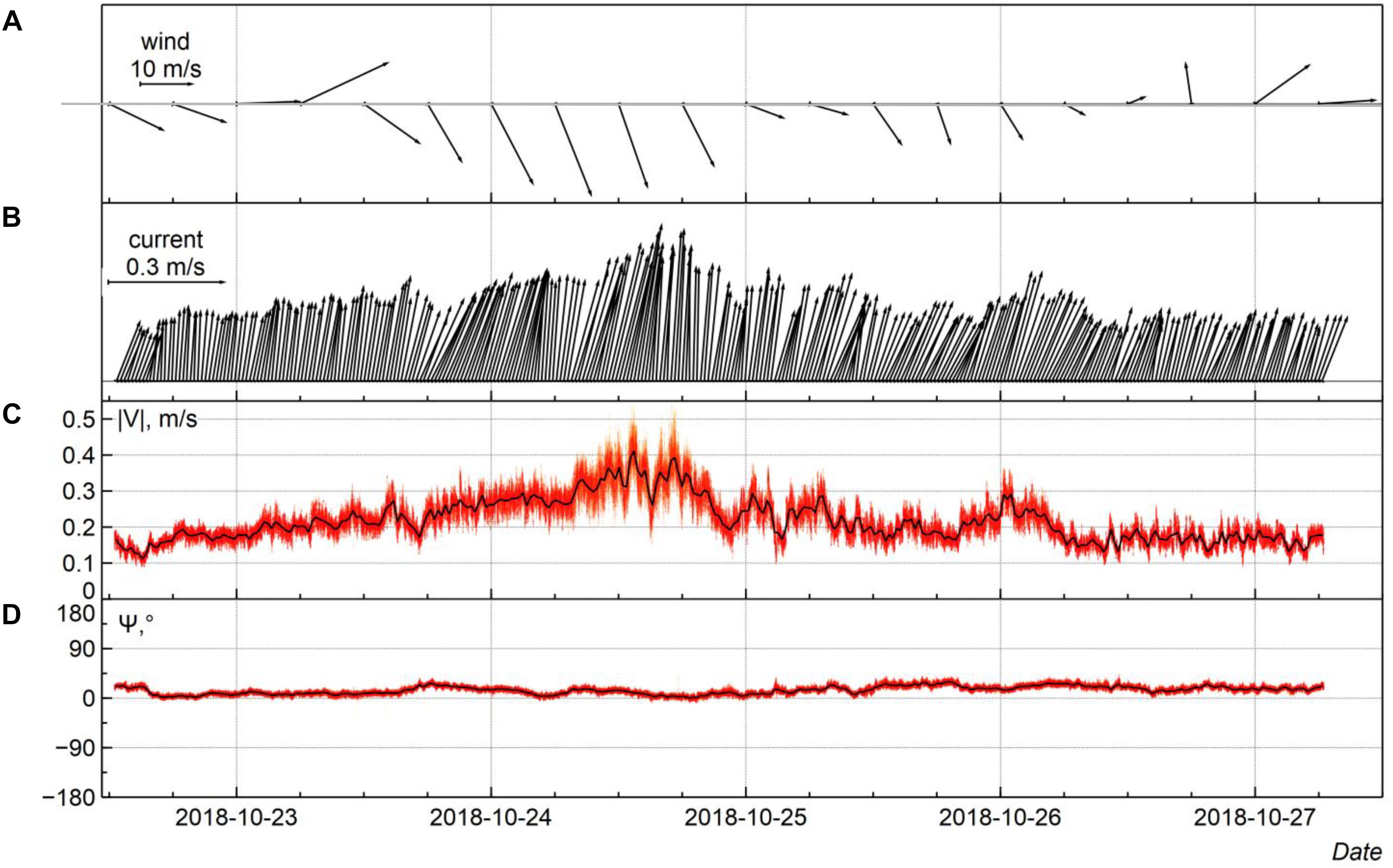
Figure 12. The bottom current measured by TCM was installed on the eastern slope of the Hoburg Channel (see Figure 5) for the period 22–27.10.2018. (A) wind vectors with a 6 h interval for the point (19°E, 56°N) from the ECMWF database (www.ecmwf.int), (B) current velocity vectors, (C) current velocity magnitude | V| (red line is the instant current, black line is the 20 min running average value), (D) current direction Ψ relative to North and positive clockwise.

1. Why was the near-bottom current exceptionally unidirectional while its magnitude varied considerably within a range of 0.15–0.56 m/s?

2. Why did the direction of the current remain unchanged when the wind direction and force change?

3. Why was the flow not affected by inertial oscillations?

4. Why did the velocity of the NE near-bottom current increase largely (from 0.2 to 0.5 m/s) with the strengthening of the NW wind to severe gale?

5. What makes the TCM location exceptional, so that at the distance of only 0.5 m from the bottom, the flow velocity can reach values greater than 0.5 m/s?

A closely spaced CTD transect passing though the TCMs site (Figure 13) showed that TCMs were placed at the bottom in the midpoint of the eastern rim of the Hoburg Channel at a depth of 85 m, where the bottom tilt reaches a maximum value of γ = 0.0074 and the buoyancy frequency is as high as N = 0.017 s^-1. The flow near the sloping bottom in stratified media is expected to be directed along the intersection of isopycnal surfaces with the inclined seabed surface. Therefore, if the isopycnal surfaces are horizontal, the near-bottom flow will be exactly aligned to the sea depth contours (isobaths). In fact, the isopycnal surfaces are not exactly horizontal, and, therefore, the near-bottom currents are only approximately aligned to the depth contours. Looking at the bathymetric map in Figure 1 (or at the close-up in Figure 5) and the time series of the near-bottom current vector in Figure 12, one can see that the near-bottom flow was aligned to the sea depth contours, which does explain approximate constancy of the flow direction.

FIGURE 13

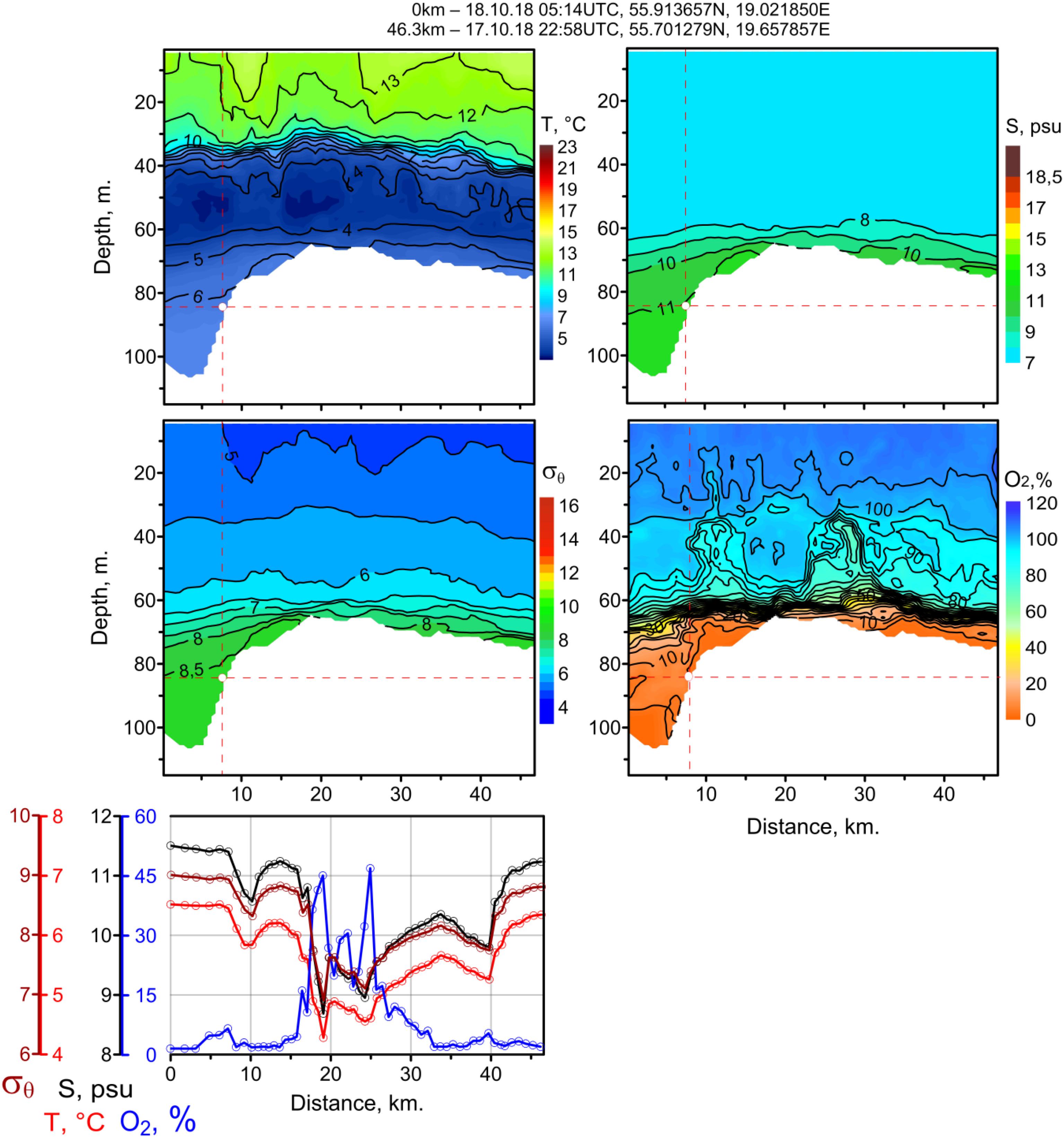
Figure 13. Distributions of temperature T (°C), salinity S (psu), density σ_θ, and oxygen saturation O₂ (%) in a transect across the eastern rim of the Hoburg Channel passing through the TCMs deployment site. Position of the TCMs on the transect is marked by a small white bullet intersected by dashed lines. Bottom panels demonstrate graphs of the same parameters in the bottom layer.

Looking at the potential density vs. distance and depth on the transect across the eastern rim of the Hoburg Channel (Figure 13), one can observe that the isopycnals in the saltwater (halocline) layer are sloping down in the western direction, implying northward geostrophic transport in the near-bottom gravity current which is in accordance with the time series of the measured near-bottom current vector shown in Figure 12. Note that for geostrophic considerations in the near-bottom gravity currents, the reference level of zero geostrophic velocity should be adopted above the gravity current layer.

The inertial motion of a fluid particle with horizontal component of velocity U in a rotating media with the Coriolis parameter f implies anticyclonic (clockwise in the Northern Hemisphere) rotation of the particle with the period 2π/f, so the diameter of the particle’s trajectory is D = 2U/f. If the particle is at a height h above the inclined bottom with the slope γ, the inertial circular motion with diameter D will be possible only if h/γ > D or h > h_i = 2γU/f, where h_i is the height of bottom layer in which the inertial oscillations are hampered by the presence of the bottom slope. Having γ = 0.0074, f = 1.21 × 10^-4 s^-1 (for latitude 56°N), and U = 0.2–0.5 m/s we get h_i = 24.4–61.0 m. The time series of current velocity presented in Figure 12 is free of inertial oscillations because it was measured at a distance of 0.5 m from the bottom, which is much smaller than h_i.

It can be seen from the bathymetric map (Figure 1) that in the vicinity of the TCM deployment point, the 70 m depth contour, which approximately depicts the lateral boundary of the saltwater reservoir in the lower layer of the Baltic Proper, turns sharply to the east, making the reservoir much wider. For this reason, the TCMs happened to be deployed in the “bottle neck” on the pathway of northward spreading saltwater. When the NW wind has grown to severe gale, the low-salinity water in the upper layer rushed to the southwest owing to the Ekman transport, causing an intensification of the oppositely directed northeast flow of the saltwater in the lower layer through the Hoburg Channel. The situation is quite similar to that of the Słupsk Furrow, where the northerly and easterly winds drive the westward transport in the upper layer and intensify the eastward transport of the saltwater in the lower layer of the Furrow, while the westerly and southerly winds result in weakening and even blocking the eastward transport of the saltwater through the Furrow (Krauss and Brügge, 1991; Zhurbas et al., 2012).

Keeping in mind that the flow velocity at h = 0.5 m above the bottom reached as large a value as U = 0.5 m/s, it seems interesting to estimate the corresponding value of the bottom friction velocity u_∗ and also the rate of dissipation of kinetic energy of turbulence ε based on the celebrated formulas of von Kármán’s “law of the wall” [e.g., Paka et al. (2013)]:

$${\mathit{u}}_{*}^2={\mathit{C}}_{\text{d}}{\mathit{U}}^2,{\mathit{C}}_{\text{d}}=\frac{{\mathit{K}}^2}{{[\ln \left(\mathit{h}/{\mathit{z}}_0\right)]}^2},\text{ε}=\frac{{\mathit{u}}_{*}^3}{\mathit{K}\mathit{h}},$$

where C_d is the drag coefficient, K = 0.4 is the von Kármán’s constant, and z₀ is the roughness parameter. The roughness parameter value adjusted in (Zhurbas et al., 2018) to fit the simulated and observed time series of bottom salinity, in particular the arrival time of the 2014–2015 MBI to BY15 (i.e., to the Gotland Deep), was z₀ = 0.002 m. Substituting U = 0.5 m/s at h = 0.5 m to the above formulas, we get u_∗ = 0.036 m/s, ε = 2.3 × 10^-4 W/kg. Such large values of bottom friction velocity and dissipation undoubtedly indicate a high level of turbulence in the gravity current of northward spreading saline water in the Hoburg Channel.

Summary and Conclusion

By participating in experimental studies of the physical processes and environmental conditions in the Baltic Sea and analyzing published materials based on the results of the general environmental monitoring, the authors concluded that the volume and completeness of the information received do not meet the requirements of the scientific community.

First, this refers to high-resolution data on mixing, ventilation and circulation of deep waters, which, if obtained, are not regular. To increase the volume and quality of such data, it is necessary to carry out additional special monitoring that meets these requirements.

According to the presented materials, we managed to solve a number of innovative tasks necessary for the organization of a special monitoring exercise in accordance with the decisions of high-level international organizations and programs, establishing and financing projects on the protection of the Baltic Sea environment (European Commission, HELCOM, Interreg Baltic Sea Region, The NATO Science for Peace and Security, et al.).

In particular:

- A new technology of field works on hydrographic transects is developed that assumes the use of standard multiparameter probes, and the repeated casts are performed from the stern of the moving vessel. The probe drops vertically, its loose tether does not spoil the uniform sink but provides fast recovery using a rather simple longline hauler. This technique is not inferior to the previous “Tow-Yo CTD” method in technical efficiency, but surpasses it in terms of the volume and quality of information, including the characteristics of a fine structure in the water column and especially in the bottom layer, requiring neither powerful winches nor specially equipped research vessels. The main requirement to the vessel is not its size but its seaworthiness. In the near future, the new method of work on the vessel could allow carrying out special monitoring of the Baltic Sea and other seas, optimal by the criterion of data price-quality.

- A possibility to carry out regular measurements of microstructure without significant restrictions on weather conditions is shown. The proposed method of working with a quasi-free falling probe equipped with a magazine to store the required amount of tether can allow measurements in any areas of the Baltic Sea at any drift speed of the vessel, as well as at slow speeds moving forward against strong winds and sea swells. Field tests carried out in the area of the Słupsk Sill showed that the advanced system allows for the determination of the basic characteristics of the microstructure and the background thermohaline stratification but requires additional currents measurements. We hope to find a solution to this task in the near future.

- A possibility to fill the gap of data on the bottom currents is shown using an improved TCM model, the serial production of which can be provided by any manufacturer of oceanographic equipment, given the serially produced main metrological components to measure the tilt and orientation of the current meter—the 3D accelerometer and electronic compass—are already commercially available.

Comparison with the reference data obtained in the IOW monitoring cruises showed that the innovative technology of field work on hydrographic transects, consuming less ship time and fuel, is nevertheless able to provide measurements of oceanographic parameters in the near-bottom layer of the quality comparable with the quality obtained at the standard drift stations.

Among the interesting findings received thanks to the innovative measurement technology are the highest ever recorded temperature of 14.3°C in the halocline of the Bornholm Basin, measured after a baroclinic inflow event of early Autumn 2018, and the high rate of dissipation of turbulence kinetic energy in the near-bottom layer filled with eastward-flowing saltwater beyond the Słupsk Sill. But from our point of view, the most interesting result was obtained using the TCM.

Our search for the site for TCM deployment was based on the results of modeling of the bottom stress velocity in the Baltic Sea (Zhurbas et al., 2018); we sought to find a location with high probability to meet large bottom stress and, therefore, large velocity of near-bottom currents. Our attention was caught by a plot on the eastern rim of the Hoburg Channel which was in accordance to the simulations (Zhurbas et al., 2018) whereby the probability to meet u_∗ > 0.005 m/s exceeded 0.5, and the plot was located within the Russian Economic Zone. Our expectations were not misplaced: the TSM deployed there for a relatively short period of 5 days did record a current velocity of more than 0.5 m/s within a 1 m above the bottom depth of 85 m, which corresponds to large values of bottom friction velocity and a dissipation rate of u_∗ = 0.036 m/s, ε = 2.3 × 10^-4 W/kg. Such a large value of the bottom friction velocity and dissipation rate undoubtedly indicated a high level of turbulence in the gravity current of northward-spreading saline water in the Hoburg Channel.

The close inspection of the bathymetry map showed that, figuratively speaking, the TCM happened to be deployed in the “bottleneck” on the pathway of the northward-spreading saltwater. For this reason, we plan to use this location as an easily accessible polygon for future field studies of near-bottom gravity flows and related turbulence using the innovative technologies described above.

Author Contributions

VP provided measurements, data analysis, and interpreted field data. VZ and MG carried out data analysis and interpreted field data. AOK and AAK set up the equipment, provided measurements, and processed data. SS provided measurements.

Funding

Measurements and analysis of hydrodynamic parameters were performed within the framework of the IO RAS state assignment (Theme No. 0149-2019-0013); production of inclinometers was supported by the Russian Foundation for Basic Research (Grant No. 17-05-41196); the improvement of the sounding technique, the development of the design of inclinometers, as well as the analysis of the variability of currents depending on local geographic factors were supported by the Russian Foundation for Basic Research (Grant No. 18-05-80031); analysis of the data obtained by the microstructure probe was supported by the Russian Foundation for Basic Research (Grant No. 19-05-00962); the report on the results of measurements on transects and by inclinometers at an international conference was supported by the EU INTERREG Baltic Sea Region Program 2014–2020, Project DAIMON (Decision Aid for Marine Munition).

Conflict of Interest Statement

The authors declare that the research was conducted in the absence of any commercial or financial relationships that could be construed as a potential conflict of interest.

Footnotes

1. ^https://www.nortekgroup.com/ (accessed March 15, 2019).
2. ^http://www.charlieengineering.com/portfolio-items/fishing-line-rope-haulerwinch/ (accessed March 15, 2019).
3. ^https://www.io-warnemuende.de/cruise-reports.html

References

Bełdowski, J., Jakacki, J., Grabowski, M., Lang, T., Weber, K., Kotwicki, L., et al. (2018a). “Best Practices in Monitoring,” in NATO Science for Peace and Security Series C: Environmental Security, eds J. Bełdowski, R. Been, and E. Turmus (Dordrecht: Springer).

Google Scholar

Bełdowski, J., Long, T., and Söderström, M. (2018b). “Introduction,” in Towards the Monitoring of Dumped Munitions Threat (MODUM). NATO Science for Peace and Security Series C: Environmental Security, eds J. Bełdowski, R. Been, and E. Turmus (Dordrecht: Springer).

DAIMON Project (2019). Decision Aid for Marine Munitions. Available at: https://projects.interreg-baltic.eu/projects/daimon-22.html (accessed March 15, 2019).

Gelumbauskaite, L. Z., Grigelis, A., Cato, I., Repecka, M., and Kjellin, B. (1999). Bottom Topography and Sediment Maps of the Central Baltic Sea LGT Series of Marine Geological Maps No. 1, SGU Series of Geological Maps BA No. 54, Scale 1:500000. Vilnius: Lithuanian-Swedish project GEOBALT.

Golenko, N., Paka, V., Golenko, M., and Korzh, A. (2008). Meso-scale water structure in the southern Baltic in the summer of 2006. J. Mar. Syst. 74, S13–S19. doi: 10.1016/j.jmarsys.2008.01.015

CrossRef Full Text | Google Scholar

Hansen, A. B., Carstensen, S., Christensen, D. F., and Aagaard, T. (2017). Performance of a tilt current meter in the surf zone. Coast. Dyn. 218, 944–954.

Google Scholar

Krauss, W., and Brügge, B. (1991). Wind produced water exchange between the deep basins of the Baltic Sea. J. Phys. Oceanogr. 21, 373–384.

Google Scholar

Matthäus, W., and Franck, H. (1992). Characteristics of major Baltic inflows - a statistical analysis. Cont. Shelf Res. 12, 1375–1400.

Google Scholar

Mohrholz, V. (2018). Major Baltic inflows statistics – revised. Front. Mar. Sci. 5:384. doi: 10.3389/fmars.2018.00384

PubMed Abstract | CrossRef Full Text

Mohrholz, V., Dutz, J., and Kraus, G. (2006). The impact of exceptionally warm summer inflow events on the environmental conditions in the Bornholm Basin. J. Mar. Syst. 60, 285–301.

Google Scholar

Mohrholz, V., and Heene, T. (2018). The Słupsk Sill Overflow – Mixing Hot Spot of the Eastward Spreading Saline Water. Available at: https://www.baltic.earth/events/helsingor2018/material/2ndBalticEarthConferenceProceedings_IBESP_No13_lowres.pdf (accessed May 13, 2019).

Google Scholar

Paka, V., Zhurbas, V., Rudels, B., Quadfasel, D., Korzh, A., and Delisi, D. (2013). Microstructure measurements and estimates of entrainment in the Denmark Strait overflow plume. Ocean Sci. 9, 1003–1014. doi: 10.5194/os-9-1003-2013

CrossRef Full Text | Google Scholar

Paka, V. T., Rudels, B., Quadfasel, D., and Zhurbas, V. M. (2010). Measurements of turbulence in the zone of strong bottom currents in the Strait of Denmark. Dokl. Earth Sci. 432, 613–617.

Google Scholar

Piechura, J., and Beszczyńska-Möller, A. (2004). Inflow waters in the deep regions of the southern Baltic Sea — transport and transformations. Oceanologia 46, 113–141.

Google Scholar

Piechura, J., Walczowski, W., and Beszczynska-Möller, A. (1997). On the structure and dynamics of the water in the Słupsk Furrow. Oceanologia 39, 35–54.

PubMed Abstract | Google Scholar

Rak, D. (2016). The inflow in the Baltic proper as recorded in January–February 2015. Oceanologia 58, 241–247.

Google Scholar

Rak, D., and Wieczorek, P. (2012). Variability of temperature and salinity over the last decade in selected regions of the southern Baltic Sea. Oceanologia 54, 339–354.

Google Scholar

Sanderson, H., Fauser, P., Thomsen, M., Vanninen, P., Soderstrom, M., Savin, Y., et al. (2010). Environmental hazards of sea-dumped chemical weapons. Environ. Sci. Technol. 44, 4389–4394. doi: 10.1021/es903472a

PubMed Abstract | CrossRef Full Text | Google Scholar

Zhurbas, V., Elken, J., Paka, V., Piechura, J., Väli, G., Chubarenko, I., et al. (2012). Structure of unsteady overflow in the Słupsk Furrow of the Baltic Sea. J. Geophys. Res. Oceans 117:C04027. doi: 10.1029/2011JC007284

CrossRef Full Text | Google Scholar

Zhurbas, V., Väli, G., Golenko, M., and Paka, V. (2018). Variability of bottom friction velocity along the inflow water pathway in the Baltic Sea. J. Mar. Syst. 184, 50–58.

Google Scholar

Zhurbas, V. M., Paka, V. T., Golenko, M. N., and Korzh, A. O. (in press). Transformation of eastward spreading saline water at the Słupk Sill of the Baltic Sea: an estimate based on microstructure measurements. Fundamentalaya i Prikladnaya Gidrofizika 12.