Morphological Evolution of an Intertidal Area Following a Set-Back Scheme: A Case Study From the Perkpolder Basin (Netherlands)

Introduction

Tidal flats are intertidal, non-vegetated, soft sediment habitats generally composed of mud and sand (Dyer et al., 2000), often backed by salt marshes that grow at higher elevations within the intertidal fringe. Coastal salt marshes are usually found along low-energy and temperate coastlines (Allen, 1992; Adam, 2011), except for the extensive mangrove forests that are located at tropical latitudes (Odum et al., 1982). Salt marsh plants, mostly herbaceous halophytes, are adapted to tolerate regular saltwater inundation, especially the species that colonize the low-elevated parts (Pratolongo et al., 2019).

Despite the fact that salt marshes were historically considered as a source of insalubrious conditions (humidity, mosquitoes) and as land unsuitable for agriculture (Boavida, 1999), they can offer numerous ecosystem services. Several studies have discussed the benefits derived from these environments to nature and mankind: (i) they support fisheries as they host economically and ecologically important fish species (Boesch and Turner, 1984; MacKenzie and Dionne, 2008; Barbier et al., 2011); (ii) they play a role in the carbon cycle as they are able to shift carbon sequestering from the short-term (10–100 years) to the long-term (1000 years) (Mayor and Hicks, 2009); (iii) they can host leisure activities and have an important role in local cultural aspects (Weis, 2016). The decline of these environments during the last 50 years has caused an important loss of ecosystem services (Millennium Ecosystem Assessment, 2005). Nevertheless, recent assessments on the future of salt marshes are quite controversial. In fact, global-scale predictions suggest that the capacity of marshes to recover against sea-level rise are overestimated (Nardin and Edmonds, 2014; Crosby et al., 2016; Spencer et al., 2016), but local-scale assessments concluded the opposite prediction (Kirwan et al., 2016). The reason behind this discrepancy is that large-scale assessments do not consider the biophysical feedback mechanisms that are included instead in local-scale models (Kirwan et al., 2016). Several local-scale studies demonstrated that coastal wetland loss can be avoided by using nature-based adaptation in coastal management solutions (Schuerch et al., 2018).

One of the most important roles of salt marshes is coastal protection, as they are able to attenuate wave energy and to consequently reduce the flood hazard (Bouma et al., 2014). Many studies demonstrated the effect of vegetation and wetlands on wave impact reduction (Möller et al., 2014; Smolders et al., 2015; Vuik et al., 2016) and storm surge (Stark et al., 2015; Leonardi et al., 2018).

Nature-based solutions are to be preferred to conventional coastal defences because they are effective and have a reduced cost if compared to traditional approaches (Koch et al., 2009; Borsje et al., 2011; Temmerman et al., 2013). In order to support the efficient design of nature-based solutions, a deep understanding of feedback effects between biotic (e.g., vegetation) and non-biotic factors is needed.

Previous studies focussed on established, evolving or deteriorated salt marshes; few works analyzed the processes acting on newly developed salt marshes. Several works defined how hydrological and sedimentological processes influence topographic evolution of the marsh in response to sea level rise, with surface growth following an asymptotic law (Pethick, 1981), and how the hydroperiod spatially and temporally changes sediment accretion and accumulation (Cahoon and Reed, 1995). Furthermore, several studies discussed the adaptation capacity of salt marshes to keep pace with sea level rise (Stevenson et al., 1986; van Wijnen and Bakker, 2001; Schuerch et al., 2013, 2018; Crosby et al., 2016; Kirwan et al., 2016; Spencer et al., 2016). Mathematical models have been implemented to describe sediment transport inside salt marshes and tidal creeks (Kirwan et al., 2010; Green and Hancock, 2012; Reimer et al., 2015), and biological parameters have been introduced to explain how the eco-geomorphological state of marshes influences their contribution to sediment budgets (Stark et al., 2017). In this type of environment, sediment deposition is influenced by a number of factors, such as seasonal conditions (Reef et al., 2018), sediment availability and grain-size distribution (Schuerch et al., 2014), storm frequency and intensity (Schuerch et al., 2012).

Despite our current knowledge of hydrological and sedimentological processes on well-developed salt marshes, there have been few observations and experiments concentrating on the mechanism of salt marsh creation (Gunnell et al., 2013). A better understanding of how a salt marsh develops is necessary to estimate the future distribution of vegetation as well as the time required to observe the transition from tidal flat to marsh environments, natural or artificial.

The capacity of predicting salt marsh development is also important to understand if a “set-back” approach is feasible, i.e., the environment is free to develop without any human intervention, such as building new coastal structures to control the process.

The existence of salt marshes is critically dependent on how fast sediment accumulates with respect to sea level rise (Redfield, 1972; Orson et al., 1985; Schuerch et al., 2012). Using 40 years of study of salt marshes in the Wadden sea (Netherlands), Bakker (2014) evidenced that a natural salt marsh forms when a mud or sand flat rises through vertical accretion until it lies just below the Mean High water Tide level (MHT), so that it is submerged twice a day for several hours and it is dry the rest of the time.

In the current study, this concept will be applied to verify the possibility to predict the future evolution of a young, artificially created, tidal flat at Perkpolder (Zeeland, NL).

The overall aims of the study are: (i) to understand the patterns of morphological variation of the tidal flat; (ii) to describe patterns of sediment accretion across the most elevated parts of the flat; (iii) to predict where and when an optimal elevation will be reached for the establishment of permanent vegetation; (iv) to define the morphological evolution of an artificial inlet that was dredged to establish communication with the estuary.

Study Site

The study area is located in Perkpolder, a previously reclaimed area in the municipality of Hulst, in the province of Zeeland (Netherlands) (Figure 1). This site is part of the Scheldt Estuary, characterized by a length of 355 km from source to mouth, with a total catchment area of 21863 km². About 10 million people live in the river basin (Meire et al., 2005). According to the geometry of the estuarine channel and its hydraulics, the Scheldt is divided into three different zones: a narrow part dominated by freshwater from Gentbrugge to Rupelmonde, an intermediate zone from Rupelmonde to Hansweert, and a wide and well-mixed part from Hansweert to the mouth (Nihoul et al., 1978). The mud of the Scheldt Estuary has both marine and terrestrial origin; the ratio between these two muds of different sources is highly variable, partially due to the variation in the location of the turbidity maximum (ETM), and partially due to changes in sediment load of the tributaries of the Scheldt (Swart, 1987; Wartel et al., 1993; Brinke, 1994; Chen et al., 2005). The sediment transport rates depend on the seasons and on the tidal cycles. The suspended concentration is usually higher during the flood and during spring tides than during ebb and neap tides. In winter, the suspended concentration and the tidal amplitude are better correlated than during the summer, and the maximum concentration occurs one tide after the highest tide. These seasonal variations are connected to several processes, like changes in freshwater discharge, temperature, land erosion, and, in a less significant way, wave-induced resuspension (Fettweis et al., 1998). The study area falls in the mid-part of the estuary, the most important for sediment transport. The strong tidal currents, combined with the occurrence of flocculation due to the mixing of tidal and riverine water masses, as well as residual currents, increase the residence time of the suspended material, reaching values from hundreds of milligrams per liter to a few grams per liter (Chen et al., 2005). The mean tidal range of the estuary varies from about 3.8 m at Vlissingen (at the mouth) to about 5.2 m at Antwerp (78 km upstream); thus, most of the Western Scheldt is meso-tidal. Current velocities are up to 1–2 m s^–1 in the main channels, for an average tidal range. The mean Spring tidal range of the study area is about 5 m (Claessens and Belmans, 1984).

FIGURE 1

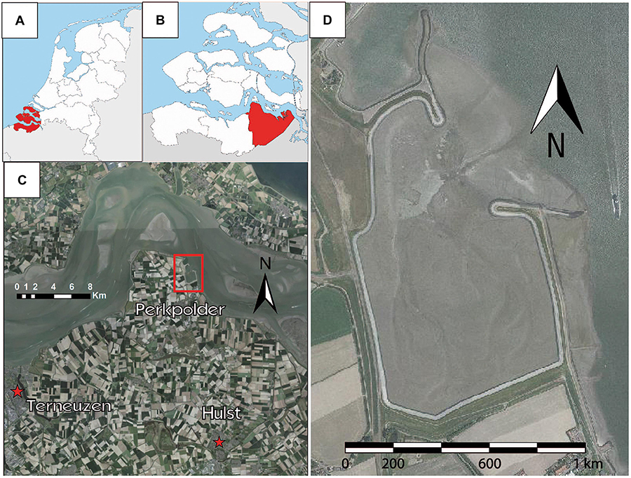
Figure 1. (A) Map of the province of Zeeland and (B) the municipality of Hulst. (C) Location of the Perkpolder tidal basin within the Scheldt Estuary and (D) 1:15000 orthophoto from the Province of Zeeland of the area, captured in June 2017.

The study area is a 75-hectares tidal flat (Figure 2), created as a cooperation project between Rijkswaterstaat (Dutch Ministry of Infrastructure and the Environment) and the regional government. This project, started after the closure of the ferry service between Kruiningen (Zuid-Beveland) and Perkpolder (Zeeuws-Vlaanderen) in 2003, was named Plan Perkpolder, and it aims at prompting the socio-economic development of the area by combining the construction of recreational facilities and natural environments. One of the most important objectives of this plan was to recreate a tidally-dominated natural ecosystem (Boersema, 2016). This polder was originally dammed in 1210 and the land was reclaimed for crop growth and for building small villages. Subsequently, the land behind the dike subsided, dropping to an elevation below mean sea level. Due to the proximity of the Schaar van Ossenisse, a deep channel in the Western Scheldt, the coast was susceptible to dyke failure. In 1841, a new dyke of about 1 km was built along the coast, but half of it was quickly lost.

FIGURE 2

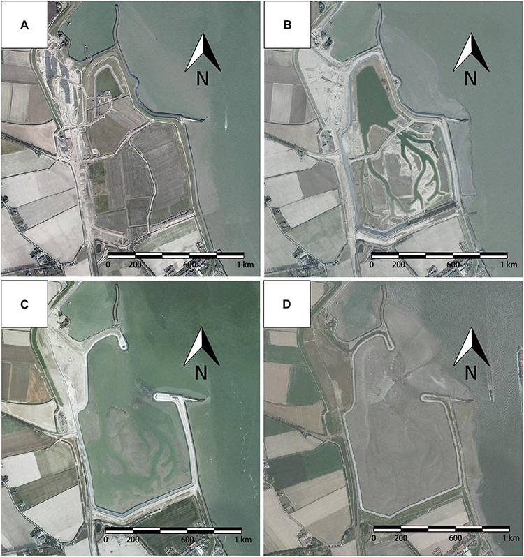
Figure 2. Orthophotos at 1:15000 scale of the Perkpolder basin from the maps of the province of Zeeland; (A) before works in March 2014, (B) shortly before the opening of the inlet in March 2015, (C) in March 2016 and (D) in June 2017.

The Perkpolder tidal flat is divided into three zones: the foreshore outside the basin, the pond, and the inner part, where several creeks were dug during the restoration project. There are two main creeks of about 40 m in width; they divide southwards into narrower branches of about 30 m in width, reaching a total length of about 800 m. On 25 June 2015, the dyke was breached (Figure 2B) and the salt water of the Western Scheldt started to flow in the basin covering the whole tidal flat. The inlet has a width of about 300 m and its bottom is located at a height of about 0–1 m NAP. The inlet is submerged during high tide only, except for the central part, which is deeper, being at −0.8 m NAP. This deeper permanent channel has a width of about 10 m and allows continuous water exchange between the pond and the open estuary.

Field observations, the basin structure, and the presence of a dyke ring support the idea that the flood and ebb currents were the principal agents causing morphological changes, as wave action is negligible given the small internal fetch and the unlikely penetration across the shallow inlet (Figures 2C,D). Field observations after the opening also suggest that benthic macro fauna rapidly started to colonize the area, providing food for bird communities.

Methodology

Morphological Analysis

The monitoring strategy aimed at identifying the evolution of the area immediately after the opening of the inlet. Following previous authors (Thomas and Ridd, 2004; Nolte et al., 2013), sedimentation patterns are analyzed in a short-time interval, to obtain data from a spring-neap tidal cycle (15 days), as well as over a longer-period (32 days). Additionally, from June 2015 to January 2017, seven multi-beam datasets of the inlet area were obtained from surveys undertaken by Rijkswaterstaat. A cross-section (Figure 3) was digitized across the inlet to see its evolution through time, assessing changes in width, depth, and wetted area.

FIGURE 3

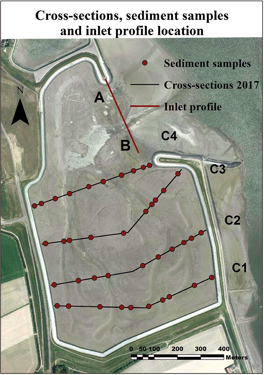
Figure 3. DGPS cross-sections (C1–C4), inlet profile (A–B) and location of sediment samples.

In order to assess the morphological evolution of the tidal flat through time, three Lidar surveys, with a 2 m x 2 m resolution, were used. The surveys were performed by Rijkswaterstaat. As the unprocessed point clouds were not supplied, a direct evaluation of the vertical accuracy could not be undertaken. Notice that accuracy depends on the Lidar sensor resolution (Wehr and Lohr, 1999), the landscape features of the intertidal environment (Evans et al., 2019) and the presence of vegetation (Hladik and Alber, 2012). In low and high marshes, the vegetation clearly influences the accuracy, causing errors from 0.1 to 0.45 m (Morris et al., 2005; Rosso et al., 2006; Wang et al., 2009; Schmid et al., 2011; Millard et al., 2013), requiring corrections to DTMs. As in Perkpolder, the tidal flat is completely un-vegetated and with no large bed features, it was considered unnecessary to re-process further the DTMs. As shown by Fernandez-Nunez et al. (2017), bare mud in Lidar surveys is represented with very high accuracy (0.04–0.09 m), and the effects of corrections in this kind of environment can be meaningless or even increase the error.

The first survey was undertaken in June 2015, in correspondence with the opening of the inlet; the second survey was undertaken in April 2016, and the third one in February 2017. Two RTK-DGPS fieldwork campaigns were performed on 12–15 June and 6–8 December 2017 (Figure 3); the DGPS survey of June was not taken into account for morphological analysis because of its proximity with the Lidar survey of February. Four cross-sections were prepared in advance on ArcGIS software and uploaded on the GPS datalogger to collect the points along selected orientations; during the successive surveys, the points of measurements where repeated with absolute care. The spacing between the surveyed points was about 10 m, except inside the creeks, where the spacing was about 5 m or less; the horizontal and the vertical accuracy was sub-centimetric. The adopted datum is the NAP (Normaal Amsterdam Peil), while the coordinate system is the Amersfoort/RD new. Data was manipulated in the ArcGIS software using “natural neighbor” as an algorithm of interpolation to create the DTMs. To evaluate the rate of sediment accretion and volume gain/loss, the datasets were processed with the Geomorphic Change Detection (GCD) tool of Wheaton et al. (2010). The tool performs an analysis of vertical variations and volume gain and loss, including an evaluation of uncertainty. According to Brasington et al. (2003), the individual errors of DTMs when a DoD (DEM of Difference) is made. They can be propagated as:

$$\mathrm{\delta }{u}_{\text{DoD}}=\sqrt{{(\mathrm{\delta }{\mathrm{z}}_{\text{new}})}^2+{(\mathrm{\delta }{\mathrm{z}}_{\text{old}})}^2}(1)$$

In equation (1), δu_DoD is the propagated error, while δz_New and δz_Old are the individual errors of each DTM. Because no vertical accuracy was set-up as the unprocessed point clouds were not available, the best option was to consider a range of the individual error in this type of environment (0.04–0.09 m), implying that the error of the new DTMs ranged between 0.06 and 0.12 m. The GCD tool also allows to choose the threshold below which lower variations are considered meaningless: in this case the calculations were made considering thresholds of 0.05, 0.10, 0.15 m, and no threshold at all, as previously done by Duo et al. (2018). Because of different vertical accuracies in the datasets (e.g., Lidar vs. DGPS), the interpretation of DTM changes has higher reliability only when the same types of datasets are compared. This means that the most consistent data intervals are from the first 2 years after the inlet opening (June 2015–February 2017). To study the additional period from February 2017 to December 2017, a comparison between datasets was made (i.e., Lidar vs. DGPS), but the interpretation must be taken with extreme caution.

Particles Size Analysis (PSA)

As the same time as topographic measurements, 40 sediment samples were collected (10 samples distributed in each cross section) to characterize the particle size distribution across the tidal flat. The adopted procedure for Particle Size Analysis (PSA) follows the Italian national standard set by ICRAM (2004). The sediment samples were treated with 120 ml of Hydrogen Peroxide at 16 volumes for several days to remove the organic matter. As the Wentworth scale (Wentworth, 1922) was used to distinguish the sand from mud, the two fractions were separated using a mesh of 63 microns by wet sieving (Widdows et al., 2000). The mud was stored in large pitchers to decant, while the sand was dried at 105°C. Then, all the extraneous material (e.g., whole shells or fragments, etc.) was removed using another sieve of 1 mm and the sand content was quantified. No further analysis on the sand fraction was carried out, considering the small quantity (e.g., a few grams, less than 30% for most of the samples). After several days, the water in the pitchers was removed and the mud was displaced into smaller beakers and weighed. Part of the mud was then moved into glass petri dishes and dried at 105°C. Finally, a Micromeritics Sedigraph Analyzer was used to discriminate the percentages of silt and clay. The results of the PSA were plotted onto the Shepard’s diagram (Shepard, 1954) using the Triplot program (McHone, 1977), and a map of sediment distribution was prepared.

Measurement of Sedimentation Rate Across the Tidal Flat

Sediment deposition was measured using traps built with Perspex Petri dishes with a diameter of 9 cm and a height of 1.5 cm, placed along each cross section at 10 different spots, at the same location of the sediment samples. This kind of sediment trap has been widely used since the 1980s (Reed, 1989; French et al., 1995; Leonard, 1997; Brown, 1998; Culberson et al., 2004; Neumeier and Ciavola, 2004; van Proosdij et al., 2006). This method is highly economical and provides a good spatial resolution of sedimentation (Marion et al., 2009). Despite the fact that this technique is commonly used, there is no settled standard; the structure of the Petri dishes differs from author to author, depending on the purpose of the study, the sediment accretion rate, the occurrence of precipitation, re-suspension, or other considered variables or disturbances. The technique principally varies from using pre-weighted filters for small time periods, to using the petri dish itself as a trap, left in the tidal flat for many days or weeks, like Butzeck et al. (2015) or Temmerman et al. (2003) have done. The choice of this type of Petri dish was based on the seasonal period chosen for our study (winter-summer), the weather conditions normally experienced at the site (for example absence of torrential rainfalls), and the vertical accretion expected on this type of tidal flat from literature studies. All the traps were covered by the tide for the same time period and by all the tides, since neap tides during experimentation were high enough to cover the whole basin. The vertical accretion did not completely bury the traps, with the exception of 2 Petri dishes. These Petri dishes were located in the southern part of the area (cross-section C1) inside the creeks, where the accretion was observed to be the highest even from the analysis of the topographic surveys. Consistent rainfall was absent while traps were operating, so it did not influence the sediment deposition. In order to avoid that near-bed tidal currents displaced traps, the Petri dishes were nailed into the ground using pickets glued in the center of the dish. One spring-neap tidal cycle (15 days) and a long-period tidal cycle (32 days) were measured in two different time intervals (Figure 4).

FIGURE 4

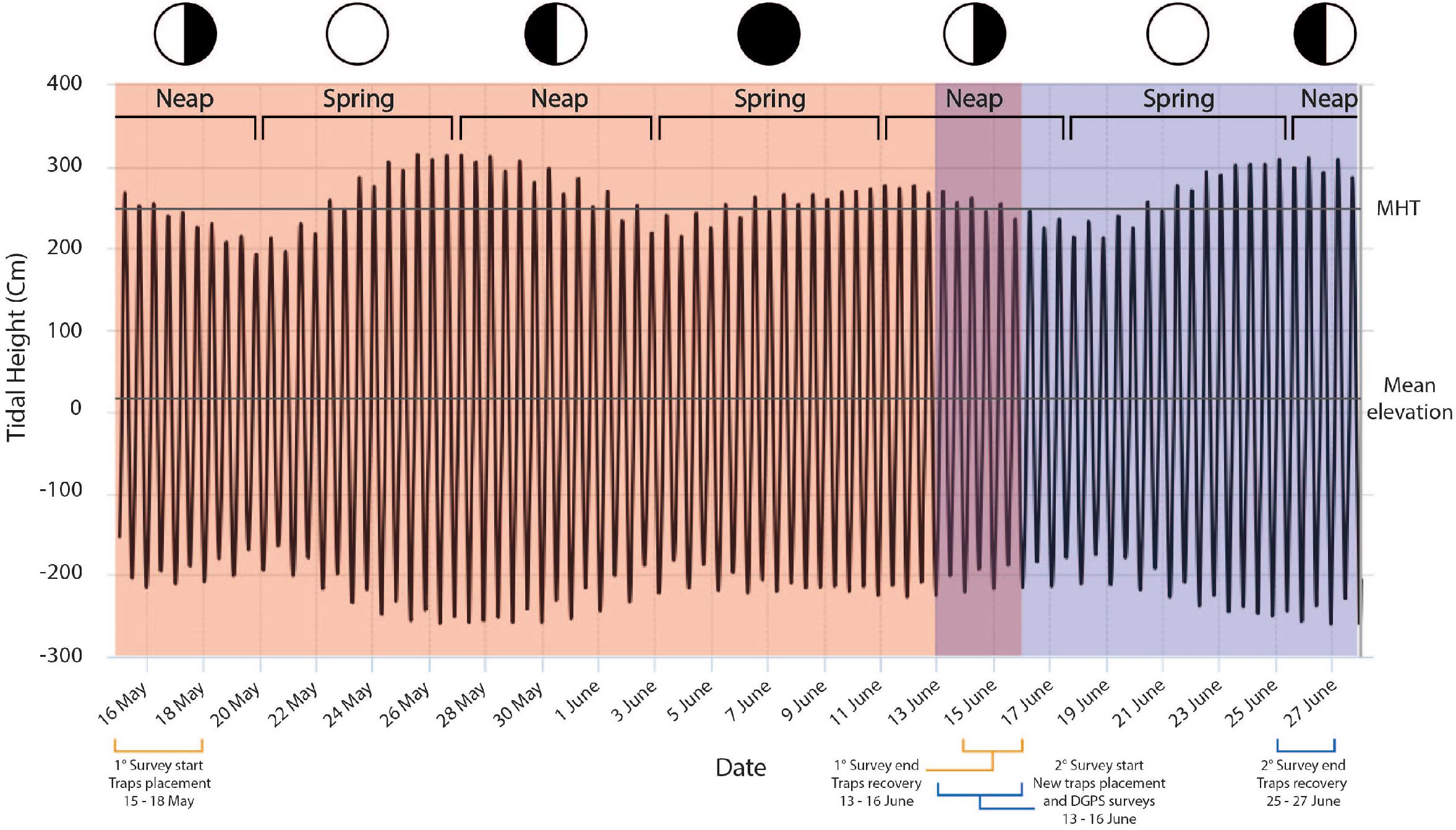
Figure 4. Neap and Spring tides during the experiments. The first experiment is from 15 of May to 16 of June; the second experiment is from 13 to 27 of June. Data from the tidal station of Walsoorden. The “Mean Elevation” horizontal line marks the mean elevation of the tidal flat.

The first measurement campaign employed 40 Petri dishes (10 per cross section) which were deployed from 15 May 2017 to 16 June 2017. A second measurement campaign employed 40 Petri dishes from 13 to 27 June, therefore covering a shorter time interval that represents a spring-neap tidal cycle. Only 57 traps out of 80 deployed were recollected after the two campaigns. The samples were dried and weighed, and the recovered sediment amount was normalized according to the days each Petri dish was left in the tidal flat to obtain values in grams day^–1. The normalization was made assuming a constant rate of deposition per day.

Loss on Ignition Analysis

Part of the bed samples was used to determine the LOI content (Loss on Ignition) according to the method of Heiri et al. (2001). The analytic procedure was divided into two phases: (1) each sediment sample was placed in an aluminum cup and then dried for a week in an oven at 80°C to remove water and determine the dry weight; (2) the dried sediment was moved into ceramic cups and weighed. The samples were then burnt at 550°C for 6 h and weighed once again to define the LOI.

Results

Morphological Datasets

Four time intervals of morphological evolution could be considered: (i) from June 2015 to April 2016; (ii) from April 2016 to February 2017; (iii) from February 2017 to December 2017; (iv) the whole period, from June 2015 to December 2017. In Figure 5 the profiles from Lidar surveys and also from DGPS surveys are shown.

FIGURE 5

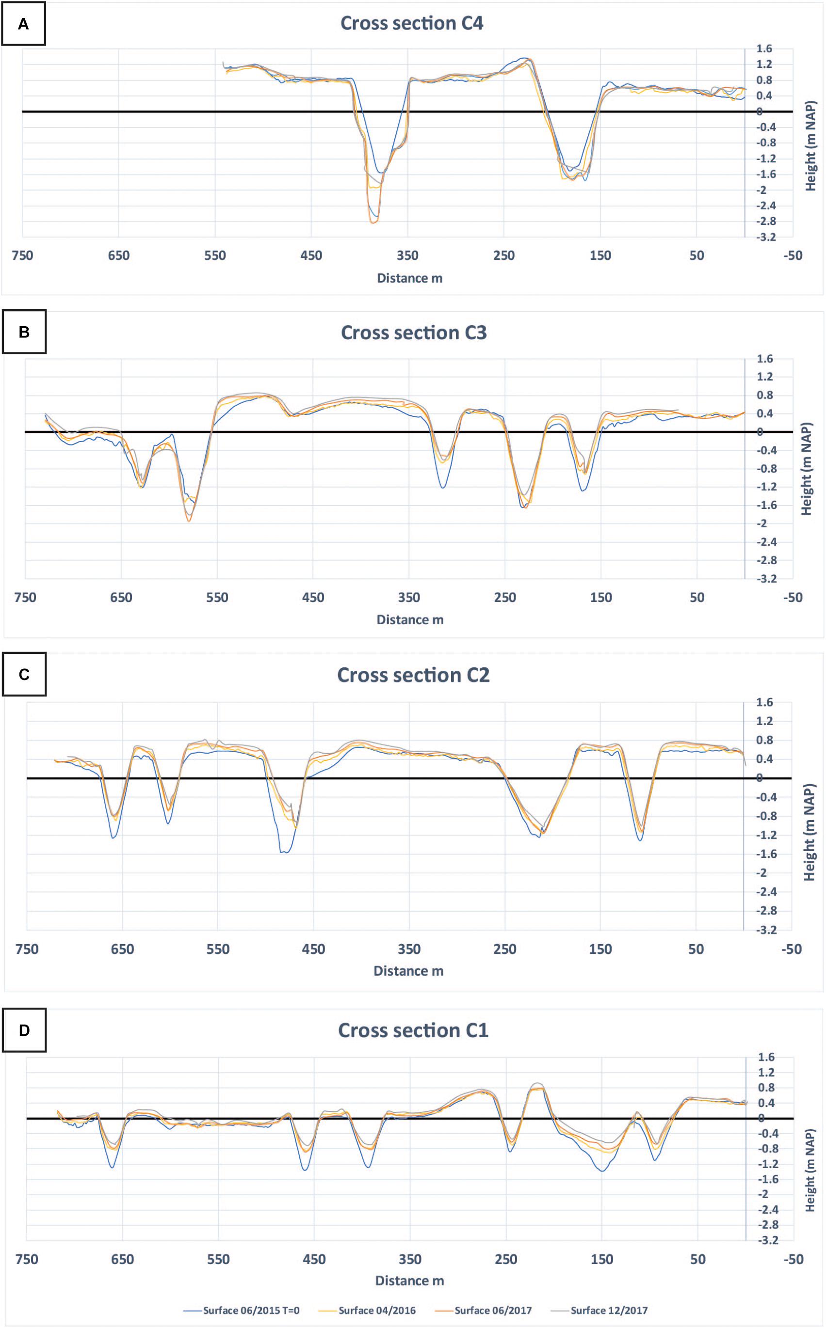
Figure 5. Cross sections from North to South (A) C4, (B) C3, (C) C2, (D) C1 extracted from Lidars (2015 and 2016) and from DGPS surveys (June and December 2017). To notice that in the graphs the survey of June 2017 is presented (orange line) to qualitatively assess bed changes but this was not used for volume calculations as it was too close in time with the preceding and subsequent surveys.

For what concerns the first interval between June 2015 and April 2016 (Figures 6A,B), the accretion is centered principally in the areas adjacent to the creeks. Overall, the accretion increases moving southwards on the tidal flat; the highest and the lowest values are located in the western creek, while the lowest parts of the creek show erosion (reaching approx. 115 cm of erosion, 11.5 cm month^–1). The accretion is not stable along the creeks, in fact in some areas, in particular in the center of the eastern creek and in the further western creek, the elevation changes are inhomogenous. On the other hand, the upper part of the flat (the southernmost part of the polder) gained a large quantity of sediment (approx. 125 cm of accretion, 12.5 cm month^–1).

FIGURE 6

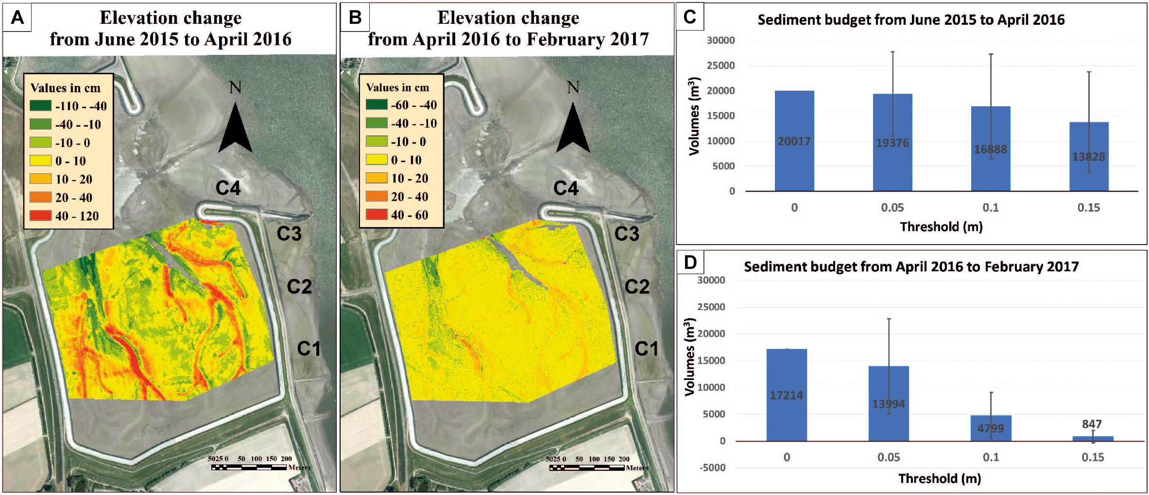
Figure 6. On the left and in the centre (A,B) elevation change computed from June 2015 to April 2016 and from April 2016 to February 2017; on the right (C,D) sedimentary budget computed for both periods considering errors of 0, 0.05, 0.10 and 0.15 m. See the text for further details on survey methodologies.

During the first 10 months after the opening of the inlet, the tidal flat experienced a great sediment gain. If we use the different error thresholds, we observed changes in the order of thousands of cubic meters: (i) with a threshold of 0.05 m the net sediment gain is 19300 ± 8400 m³; (ii) with a threshold of 0.10 m the value is about 16900 ± 10400 m³; (iii) with a threshold of 0.15 m the net gain is around 13800 ± 10000 m³ and (iv) considering no threshold at all the total sediment budget is 20000 m³. It is clear that even considering the highest threshold, the tidal flat is gaining sediment.

From April 2016 to February 2017, accretion and erosion have a similar trend; both maximum erosion and accretion reach 60 cm in 10 months, 6 cm month^–1. The highest values are concentrated in the western creek with the maximum erosion at the beginning of the creek, while the maximum accretion occurs in the central-southern part of the creek. As shown in Figure 6B, the rate of accretion seems to become stable in the whole tidal flat, with the exception of the creeks that have the highest rates. This influenced the volume calculations: during this 10 months, the total sediment budget was: (i) with a threshold of 0.05 m, 14000 ± 8800 m³; (ii) with a threshold of 0.10 m, 4800 ± 4200 m³; (i) with a threshold of 0.15 m, 850 ± 1100 m³ and (iv) with no threshold at all 17000 m³. However, it is notable that the tidal flat continues to experience sediment accumulation in a homogeneous way, with no evident morphological changes. In the last time interval, between February 2017 and December 2017, the sediment gain estimation is about 16200 m³.

The net sedimentation rates are: (i) from June 2015 to April 2016, ∼1800 m³ month^–1; (ii) from April 2016 to February 2017, ∼1400 m³ month^–1; (iii) from June 2017 to December 2017, ∼1600 m³ month^–1. Thus, the first two analyzed periods result to have quite similar sedimentation rates, characterized by a reduction of sediment gain as the tidal flat builds up. The last period is characterized by a higher rate of sediment accumulation, but this last calculation derives from the DGPS surveys and the value is probably overestimated. Considering the whole period since the opening of the inlet in June 2015 (Figure 6C), the total sediment gain on the whole tidal flat was about ∼30000 m³ from June 2015 to February 2017, of which over than 16000 m³ estimated from February to December 2017.

The same logic of error thresholds was employed to find the most reliable sediment accretion rate (Table 1). The rate of accretion calculated over the whole study area (i) from June 2015 to April 2016 was 6 ± 2.5 cm year^–1 (averaged using all thresholds); (ii) from April 2016 to February 2017 was 4.8 ± 3 cm year^–1 (using only the 0.05 threshold as data variability was smaller); (iii) from February 2017 to December 2017, only an estimation of 5.7 cm year^–1 can be produced. No quantification of the error can be performed as two heterogeneous datasets (DGPS vs. Lidar) were used.

TABLE 1

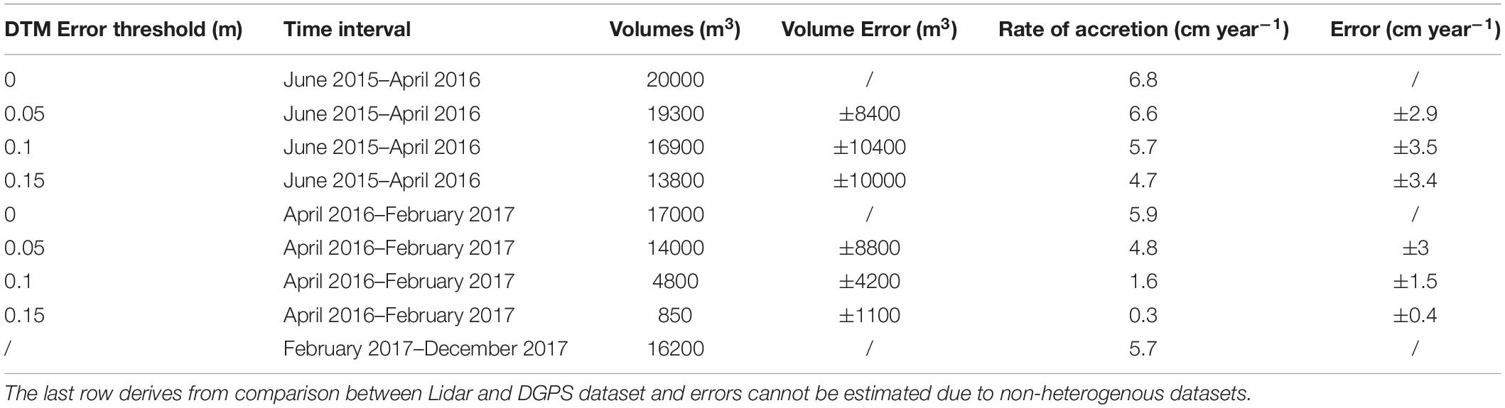
Table 1. Volume changes and rates of accretion of the study area considering different thresholds for error in the DTM.

Surface Sediment Characteristics

The granulometric classes in which the sediment samples fall are sand, silty sand, sandy silt, loam and clayey silt. Overall, the samples that contain a significant amount of sand were found next to the channels; the sand content decreases moving southwards, as showed in Figure 7A. In Figure 7B the collected samples are classified using Shepard’s diagram. Notice that pure silt and clay fractions are generally under-represented.

FIGURE 7

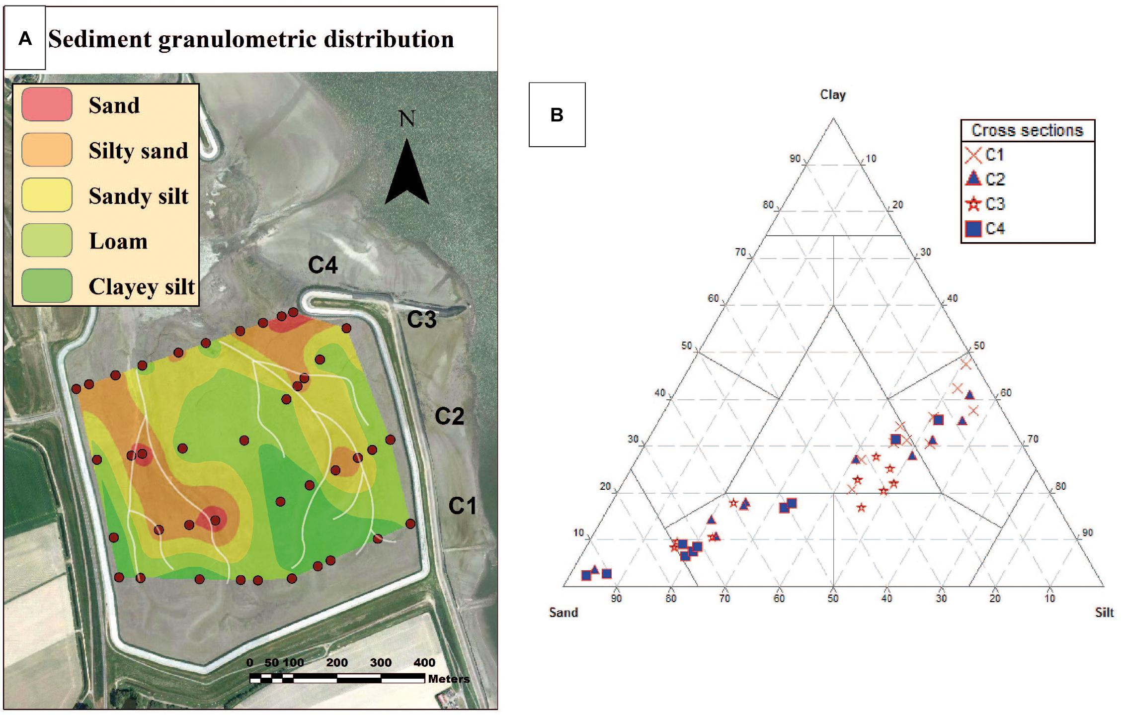
Figure 7. On the left (A) sediment granulometric distribution map derived from the analysis of 40 samples collected in Perkpolder. The map was produced using the natural neighbor interpolation. On the right (B) Shepard’s diagram shows how all samples result from a mixture of end-members of dominant sand and silt fractions.

Sedimentation Rates

No traps were completely buried, except two, implying that the collected sediment was a realistic measure of the total sediment flux. These Petri dishes were located in the southern part (cross-section C1) and inside the creeks, where the accretion measured by topographic surveys was the highest.

The data from the surveys are shown in Figures 8A,B, where values of sedimentation rates are presented in grams/m² day^–1. Due to the strong tidal flow during the first survey, only 18 Petri dishes out of 40 were recovered. Subsequently, because of the reduced density of measurements, it was decided to not interpolate the data.

FIGURE 8

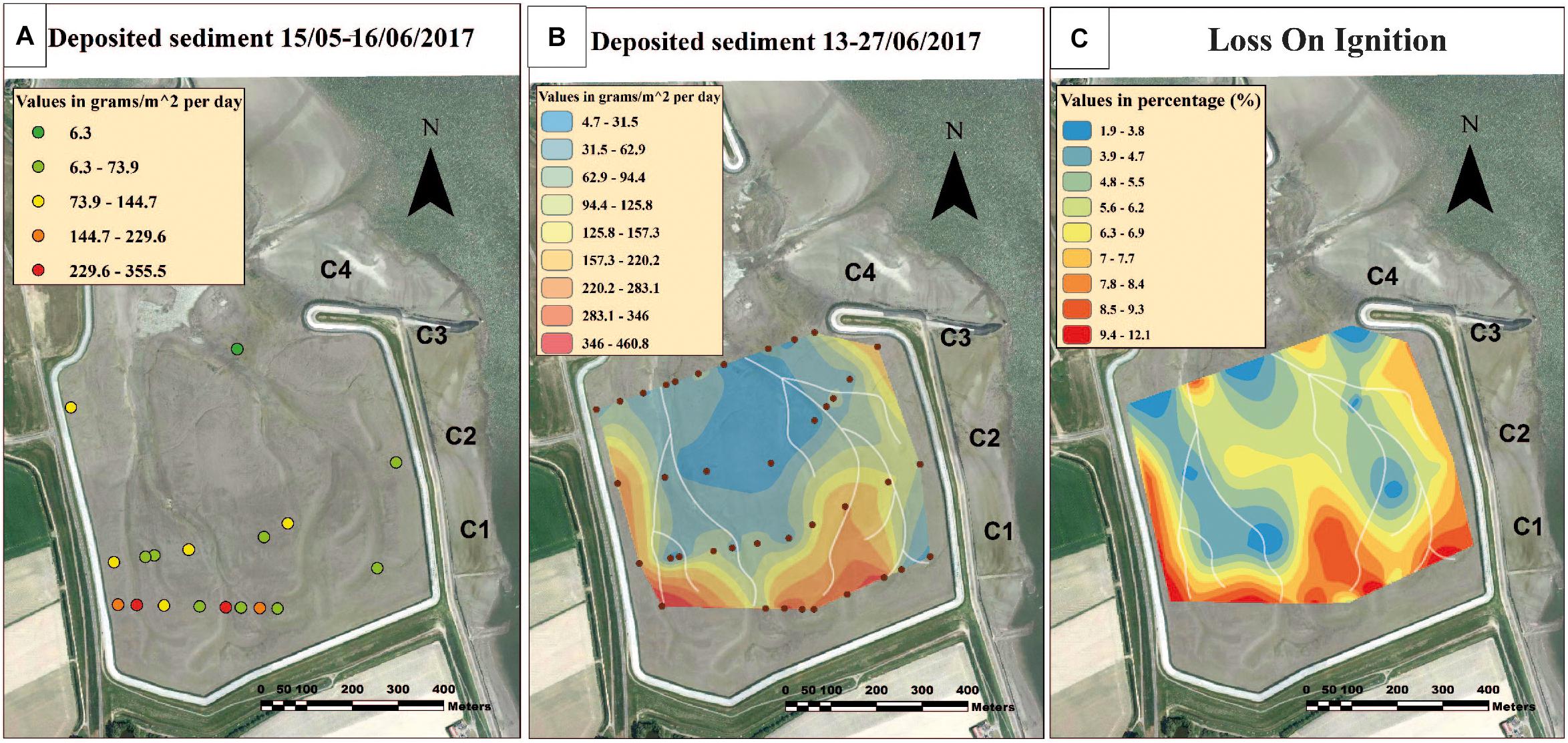
Figure 8. On the left (A) sedimentation rates from the 15 May to the 16 June 2017. In the center (B) sedimentation rates from 13 June to 27 June 2017. On the right (C) Percentage of LOI distribution. All maps were produced using the “natural neighbor” algorithm.

From 15 May to 17 June 2017 (Figure 8A), the amount of sediment trapped ranges between 6.3 g/m² day^–1 to 355.5 g/m² day^–1. The sediment amount increases moving southwards on the tidal flat.

After the second survey, performed after the spring tide of June 2017, 39 petri dishes were collected and analyzed (Figure 8B). The amount of deposited sediment per day is in the same range of the first sampling, i.e., between 4.7 g/m² and 460.8 g/m². The southernmost areas are characterized by larger accumulation, especially next to the creeks and at the border of the tidal flat. The average sediment deposition across the flat is about 111.9 g/m² day^–1 in the first survey and about 117.6 g/m² day^–1 in the second one.

Loss on Ignition

The distribution LOI is presented in Figure 8C. Overall, the organic carbon content increases moving southwards across the basin. The greatest amount is distributed around the edges, next to the dyke, and in the central area. Clayey silts contain the highest concentration of organic carbon, reaching values around 8.39–12.07%. The lowest values of 1.85–4.74% are located next to the creeks, associated to sandy sediments.

Inlet Morphology

The Dutch Ministry of Public Works (Rijkswaterstaat) supplied eight multi-beam surveys, with a cell size of 1 m x 1 m, performed between June 2015 and January 2017 (respectively 25 June 2015, 30 July 2015, 17 September 2015, 8 January 2016, 19 April 2016, 20 July 2016, 31 October 2016, 27 January 2017). For each survey, the rate of change of the width, depth, and area of the cross-section of the inlet was calculated.

The width was calculated at the bankfull, choosing as boundaries the points of increasing slope as shown in Figure 9A. The depth of the thalweg was measured considering the differences of heights between the vertical position between two time intervals. Changes in inlet characteristics were calculated by dividing one observation by the previous one. Therefore no change equals to 1, width or depth reduction is represented by values <1, and width or depth increase by values >1. In Figures 9B–H the profile changes from June 2015 to January 2017 are presented.

FIGURE 9

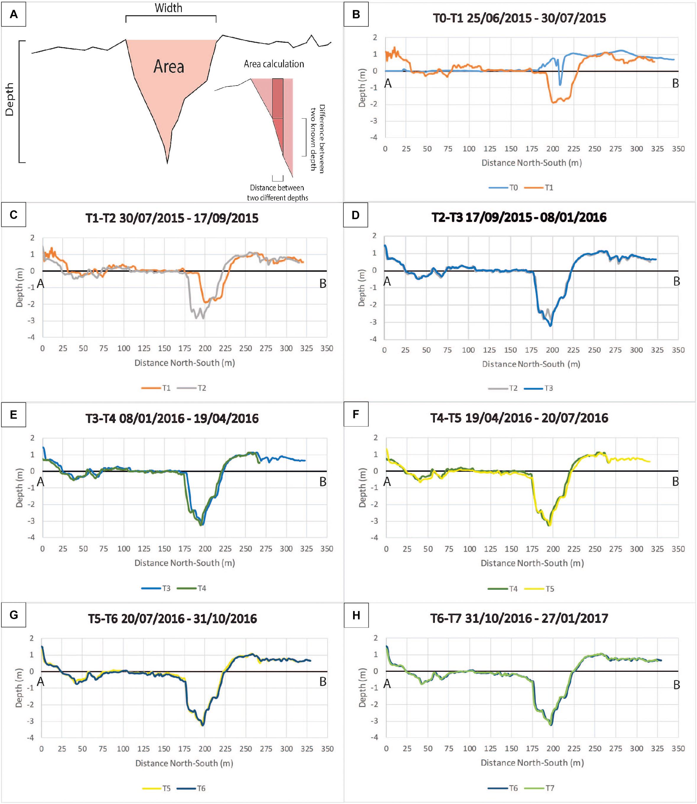
Figure 9. (A) Scheme of the calculated parameters and (B–H) profile changes from the opening of the inlet in June 2015 to January 2017.

As shown in Figure 10, after 2–4 months the rate of change slowly decreased, and after 6–8 months the inlet became almost stable.

FIGURE 10

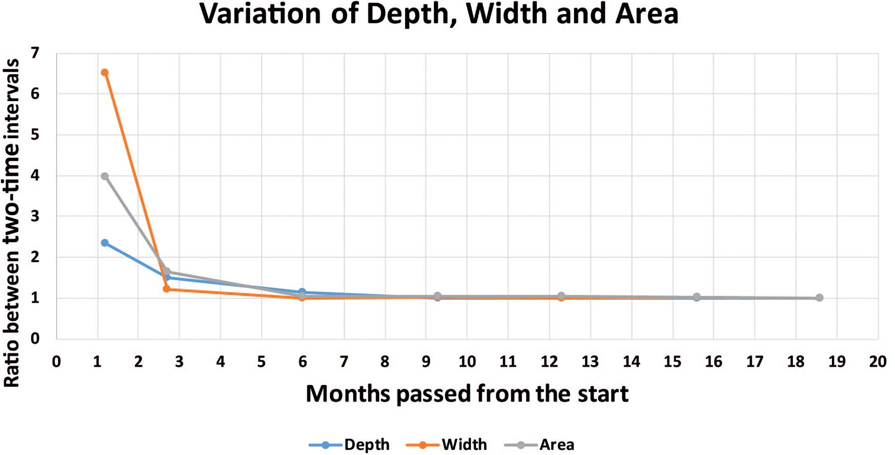
Figure 10. Variation of depth, width and cross-section of the inlet expressed as the ratio between two-time intervals from June 2015 to January 2017.

Discussion

Sedimentological Characteristics of the Tidal Flat

From a sedimentological point of view, the conditions found on this reconstructed tidal flat reflect the typical characteristics of back-barrier flats as outlined by Friedrichs (2011); the pattern of the sediment distribution, defined by coarser sediment in the creeks and on lower flats grading to finer sediment on upper flats reflect the hydrodynamic energy level and sediment supply (Mai and Bartholomä, 2000). As the dominant grain size is silt and clay, defining this as a muddy flat, the presence of coarser sediment in the creeks could be exclusively related to higher peak tidal velocities (Grabemann et al., 2004). In turn, the dominance of muddy sediment in the upper flat may depends on the location of the maximum flood line compared to the tidal flat elevation (Gadow, 1970). Because of the high tidal range, the tidal flat of Perkpolder is completely covered by the water and completely dried every day, with the exception of the northern part of the creeks. Consequently, the proximity to the creeks reflects the higher energy of the flow, allowing the transport of the coarser (sand) sediment as bedload, while the other parts of the tidal flat are characterized by fine suspended sediment due to a lower hydrodynamic regime. Furthermore, due to the reduced fetch of the basin enclosed by the dyke, it is conceivable to consider wave action not very significant, therefore the distribution of the grain size can be directly related to the peak tidal flow (Amos, 1995). Another important aspect to consider is the source of the sediment deposited inside the polder. The increasing sediment budget and the quick equilibrium state reached by the inlet strongly support the hypothesis that the sediment derives from outside the basin, also favored by the proximity of the tidal flat to the tide-dominated ETM (Nihoul et al., 1978; Chen et al., 2005). However, it must be taken into account that before the opening of the inlet, the nature of soils used for agriculture was indeed predominantly sandy. As erosion rates resulted to be more pronounced in the Northern part of the tidal flat, the higher percentage of sand in the samples could derive from the reworking by tidal currents of the original agricultural soils. It is also noticeable, as expected, the similarity in the distribution of LOI with the particle size distribution. Low values of LOI coincide with the location of coarser sediment, an indicator of higher tidal currents. The association between fine sediments and high values of organic matter is found in locations with weak hydrodynamic regimes.

Sediment Budget of the Tidal Flat

Overall, the sediment budget of the tidal flat is positive and the speed of accretion, after a very rapid onset immediately after basin opening, seems to have slightly decreased toward the end of the monitored period. During the first period of monitoring, the vertical changes were remarkable, meaning that all error thresholds could be considered as they were smaller than the order of change. Thus, the sediment budget was obtained as the average between the volumes calculated using all thresholds, resulting as ∼22000 m³ year^–1, that is, ∼1800 m³ month^–1; the second period also had a positive sediment budget, but Vertical variations are smaller than the first period and most of them were lower than the error threshold of 0.10–0.15 m. Thus, only the threshold of 0.05 m was used. The sediment budget decreased to ∼16800 m³ year^–1, equivalent to ∼1400 m³ month^–1. Finally, the volumes derived from the last period can only be considered as a gross estimate of how the tidal flat is developing, considering that two different techniques were compared (DGPS vs. Lidar). In these last 10 months the sediment gain was ∼19000 m³ year^–1, so 1600 m³ month^–1; the sediment budget of the tidal flat is still positive and the orders of volume accretion are comparable.

The accretion occurs in different areas of the tidal flat, but mostly in the creeks and at its edges. It is interesting to note that the sedimentation rate from the traps deployed during the Spring tidal cycle of June and the tidal cycle of May – June is quite the same (111.9 g/m² vs. 117.7 g/m²), adding reliability to the figures.

From a morphodynamics viewpoint, this “artificial” tidal flat presents an unusual behavior compared to natural ones. The most evident difference is in the creeks. Natural creeks of young marshes are typically characterized by a deepening and enlarging phase, caused by the increase in flow resistance on the marsh platform which concentrates the flow in the channel (D’Alpaos et al., 2006). The opposite condition is found in this study area, where the creeks are filling up. This is clearly visible in Figure 4, except for the cross section C4 which is located at the beginning of the creeks, where erosion is dominant, caused by high current velocities. On the other hand, the work of D’Alpaos et al. (2006) relates to an environment where vegetation starts to be present, while here there is no evidence of features (e.g., large bedforms, pioneering vegetation, bioconstructions) that could cause spatial changes in flow resistance. One could speculate that while the flow is inside the creek, velocities remain high, favoring the transit of consistent quantities of sediment. As the tide rises and overspills the creek banks, the expansion of the flow decreases its speed and the heaviest particles transported as bedload (e.g., sand) quickly settle inside the creek, while the fines are transported in suspension across the flat and settle in its upper part when slack tide occurs.

At last, on the basis of the inlet morphological analysis, the main channel that connects the tidal flat to the sea has become nearly stable, possibly providing a stable route for sediment input from the open estuary to the tidal flat. From a management viewpoint this is an important aspect, as future designs of similar schemes could benefit from this successful attempt to allow the system to reach an equilibrium with no intervention by man after the initial dredging.

Salt Marsh Formation

According to Bakker (2014), the conventional limit between salt marsh and tidal flat is defined by the Mean High Tide, obtained by averaging between the Mean High Spring Tide and the Mean High Neap Tide. On the basis of the tidal records of the year 2016 at the Walsoorden tidal station, for this part of the estuary this limit can be identified at about +2.53 m NAP. All the Lidar maps showed that the highest elevation ranged between +0.8 m NAP and +1.10 m NAP, exception for small spots that reached +2.30 m NAP. Thus, the tidal flat has a low elevation and it is still far from becoming appropriate for salt marsh development as the basin is constantly submerged by the tide. If the highest elevation portions are masked after choosing an arbitrary value (e.g., elevation higher than 50 cm above NAP), and a specific accretion map of these areas is created (Figure 11A), it becomes evident that the sediment is filling the lower areas, even if accretion values of Figure 11B are slighty smaller than the previous in Figure 11A. This mechanism of growth is typical of tidal flat and salt marshes and it was described by previous studies (e.g., Leonard, 1997; Allen, 2000; Temmerman et al., 2004).

FIGURE 11

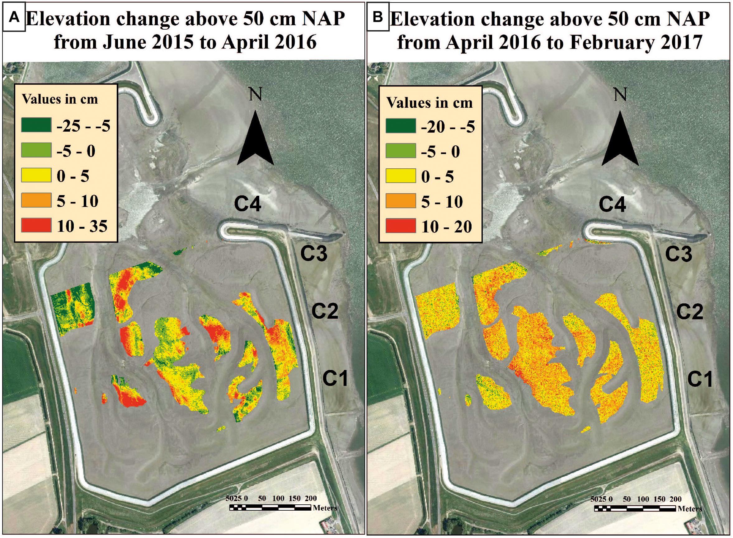
Figure 11. On the left (A) elevation changes from June 2015 to April 2016 and on the right (B) from April 2016 to February 2017.

The most elevated areas are located in the center and at the borders (North-West and North-East principally) (Figure 11B). In order to find how many years will be necessary for the tidal flat to reach the Mean High Tide at +2.53 m NAP, the best compromise was to consider the vertical accretion observed in these areas higher than 50 cm NAP. During the first period, from June 2015 to April 2016, the accretion rates of these areas was about 3.2 ± 1.7 cm year^–1. During the second period, from April 2016 to February 2017, the average decreased to 2.6 ± 1.5 cm year^–1. Furthermore, during the second period, the areas above 50 cm NAP became wider.

If the most elevated areas are taken into account (i.e., located in the northern areas at around 80 - 110 cm NAP), the highest rate of accretion are about 25 cm over 20 months, which means that these limited zones of the tidal flat will become a salt marsh not before a further 8–10 years, assuming that the sedimentation rate will remain constant in time. However, as already mentioned, the accretion of a salt marsh follows an asymptotic growth, consequently, the accretion will decrease in time. Considering now the whole areas above 50 cm NAP with an average of 3 ± 1.6 cm year^–1 will become a marsh after approximately more than 50 years. The north-west zone could be a good candidate but it is still too exposed to high hydrodynamic conditions and it will probably take longer than the other two areas.

It should also be taken into account that every plant species has a different vertical distribution above the high tide level (Gray, 1992). Gray et al. (1989) compared the vertical distribution of Spartina anglica along 107 transects across saltmarshes in 19 estuaries in south and west Britain, producing Eq. 2 that predicts the elevation limits for the existence of Spartina:

$$\mathrm{LL}=-0.805+0.366\mathrm{SR}+0.053\mathrm{F}+0.135{\mathrm{Log}}_{\text{e}}\text{A}(2)$$

where LL represents the lower limit of Spartina in meters above the NAP, SR is the Spring tidal Range (m), F is the fetch in the direction of the tidal flat transect (km) and Log_eA is the area of the estuary (km²). Perkpolder has a SR = 5.32 m, F = 3.30 km and the estuary area is 21863 km². Therefore, LL equals to 2.67 m. This value is slightly higher than the 2.53 m found by Gray et al. (1989) for British estuaries, meaning that here the condition for Spartina establishment could require the tidal flat to reach a higher elevation than the one identified along UK shores. It should be underlined that Gray’s equation is based on data collected on natural salt marshes in Britain, developed along open estuaries, while the tidal flat of Perkpolder is enclosed by dykes and has a limited tidal exchange through the inlet, subsequently this approach must be taken with caution and needs validation.

Comparison With Other Case Studies in the North Sea Area

Recent studies of other tidal flats showed how different accretion rates can occur despite similarities in tidal range. Widdows et al. (2004) described another tidal flat of the Westerschelde Estuary, Molenplaat, not so far from Perkpolder (around 6 km North-Westwards). This tidal flat has a sediment accretion of 2.4 cm year^–1, that is lower than the Perkpolder one. This could be related to granulometric differences between the two sites. The deposition rate is much lower on the open Molenplaat, with an average of 15 g/m² day^–1 while Perkpolder has a much larger rate, higher than 100 g/m² day^–1. The Molenplaat tidal flat is characterized by a sand percentage between 61–99%, while the tidal flat of Perkpolder is dominantly silty (as already mentioned, most of the samples have less than 30% of sand; there are only 2 samples composed of more than 90% of sand). The causes of these differences, even if the tidal range and the elevation above mean sea level are the same, could be due to a different regime of tidal currents. Molenplaat is an open tidal flat located in the mid-part of the estuary and the hydrodynamic energy is probably higher than in the Perkpolder basin, that is, instead, enclosed by the dyke ring. According to Nihoul et al. (1978) Molenplaat is located in a characterized by strong hydrodynamics.

A recent paper by Oosterlee et al. (2017) studied another natural restoration project in the salt marsh of Lippenbroek, in the internal part of the Scheldt estuary. A long-term analysis of nine years of monitoring was performed for this 8 ha wetland, demonstrating that the rate of accretion was about 2.35 cm year^–1. Even in this case, the sedimentation rates are lower than Perkpolder. The reason behind this difference could be that Lippenbroek is a tidal flat that has developed into a proper salt marsh, and a decrease in sedimentation is expected as high elevations are reached. Many authors (e.g., Pethick, 1981; Marani et al., 2007, 2010; D’Alpaos et al., 2011) showed that the accretion of a salt marsh follows an asymptotic growth that depends on sediment accretion, erosion and biomass, if it is present. Besides, this site is a Controlled Reduced Tide (CRT) marsh, with an artificially controlled tidal range (1.30 m at spring tides instead of the expected 5.40 m). Nevertheless, previous work of Vandenbruwaene et al. (2011) showed that the first year of this CTR marsh was characterized by an initial average sedimentation rate of about 6 cm year^–1, which is comparable with the 6 cm year^–1 observed during the first ten months of the evolution of Perkpolder. During the following four years, the rates of accretion of Lippenbroek decreased to less than 4 cm year^–1; similarly, the rate of accretion of the most elevated areas of Perkpolder after 20 months decreased to 4.8 cm year^–1. After nine years, the evolution and the accretion rates of the site of Lippenbroek become very similar to marshes in the UK, despite the different tidal regimes. On this basis, the accretion rates at Perkpolder could be expected to decrease in the future, reaching the values of natural marshes. An important difference is found in the mechanisms of channels formation. Vandenbruwaene et al. (2012) noticed that certain features influences channel formation, like low-elevated zones and areas with compacted polder clay. In the tidal flat of Lippenbroek, channels were easily ditched in low-elevated zones but were hampered by compacted clay. In the tidal flat of Perkpolder, this statement seems to not be applicable. In fact, channels started to develop in the northern areas, even in high elevation zones, but at the same time, they could not evolve in the southern areas, where silt-clay sediment is dominant but not compacted, according to field observations by the authors. Mud here is at times liquid to the point that during field surveys by DGPS the authors were sinking to the waist.

Cousins et al. (2017) installed numerous experimental clay-terraces on engineered sea walls in the marshes of Tollesbury and Langenhoe (Essex, South-Eastern England) from October 2012 to July 2014. After 22 months, the terraces in Langenhoe gained sediment at a rate of 6 cm year^–1, while in Tollesbury the rate was 3.3 cm year^–1. Compared to the study case of this paper, the sediment accretion rates of the Perkpolder tidal flats are slightly higher than those of the UK sites. Furthermore, the sediment deposition in the UK cases could have been controlled by the presence of vegetation. The Perkpolder basin is instead a young tidal flat, surrounded by dykes and located at around mean sea level NAP where vegetation is not yet able to grow. In Table 2 the different average rates of accretion of the study cases previously discussed are summarized.

TABLE 2

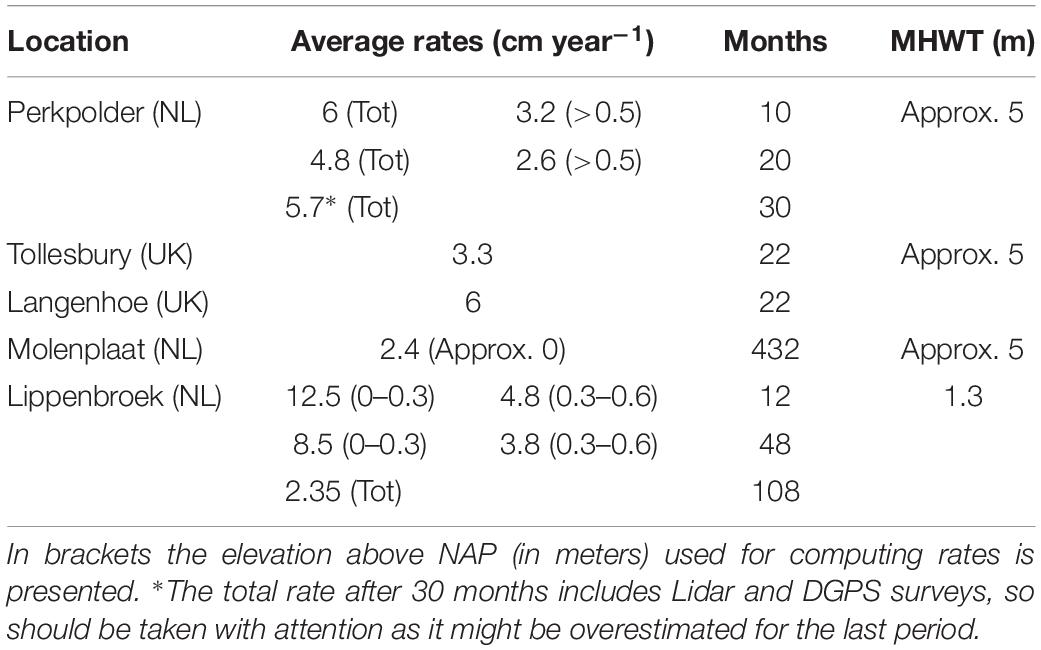
Table 2. Average rates of accretion of different study cases from the Western Scheldt (Netherlands) and South England.

Conclusion

The Perkpolder basin is a young artificial tidal flat that is still under development. Since the opening of the inlet on 25 June 2015, the site has been exposed to a semidiurnal tidal regime. Field surveys and sediment sampling proved that the basin is infilling by sand (small amounts), silty sand, sandy silt, loam and clayey silt. Organic Carbon, determined as LOI varies from 1.9% and 12.1%. Between May and June 2017, during a whole Spring to Neap tidal cycle, the deposited sediment ranged from 6.3 g/m² day^–1 to a maximum of 355.5 g/m² day^–1. During the following tidal cycle up to the Spring tide of the end of June 2017, the sediment quantity varied from 4.7 g/m² day^–1 to 460.8 g/m² day^–1. The inlet morphology analysis proved that after a quick evolution following the opening, after 6–8 months the inlet stopped its morphodynamics and reached equilibrium conditions. The total sedimentary balance was about 22000 m³ during the first year of life of the tidal flat (1800 m³ per month) and 16800 m³ during the second year (1400 m³ per month). The average accretion rate of the whole study area was about 6 cm year^–1. The most elevated areas, located 50 cm above NAP datum, like the central part of the flat and its borders, gained about 3 cm year^–1. Considering the highest regions of the study area, the conditions for initial salt marsh formation will not be established before a further 8–10 years. The portions of the tidal flat that will first become a salt marsh are mainly located in the central area, between the two artificial creeks, and in the Northeastern and Eastern areas. This study provides indication for the ecosystem-based design of innovative coastal defences, giving indications of the time required by the scheme for reaching full efficiency. The establishment of an optimal height for colonization by vegetation can be an important design guideline if a tidal flat is built by dumping of dredged material. Likewise, it provides an indication for optimal conditions if planting should be considered.

Data Availability

The datasets generated for this study are available on request to the corresponding author.

Author Contributions

RB and JP carried out the fieldwork and designed the surveys. RB analyzed the data under the supervision of JP and PC. RB and PC wrote the manuscript.

Funding

This study did not receive funding with the exception of fieldwork support from HZ University of Applied Sciences to RB.

Conflict of Interest Statement

The authors declare that the research was conducted in the absence of any commercial or financial relationships that could be construed as a potential conflict of interest.

Acknowledgments

We would like to express our deepest gratitude to the Centre of Expertise Delta Technology, a consortium between HZ University of Applied Sciences, Royal Netherlands Institute for Sea Research (NIOZ), Wageningen University and Research (WUR), Deltares, and the Dutch Ministry of Infrastructure and Environment (Rijkswaterstaat) for providing us all the data necessaries to reach the purpose of this study. The Orthophotos used for this study are available from the Province of Zeeland: https://zldgwb.zeeland.nl/geoloket/?Viewer=Luchtfotos. Thanks should also go to the numerous students from HZ University of Applied Sciences and Fabio Piazzi who helped during the fieldworks. Many thanks to Michelangelo Brunetta and Cinzia Greco for the ideas exploited to build the sediment traps. Finally, we thank Enrico Duo for the great help in introducing us to the theory of error estimations in DTM analysis. Finally, we are deeply indebted to Dr. Clara Armaroli, who provided constructive scientific criticism to an early version of the manuscript as well as language editing of the text.

References

Adam, P. (2011). Plant Life History Studies in Saltmarsh Ecology. Cambridge: Cambridge University Press, 309–334.

Google Scholar

Allen, J. (2000). Morphodynamics of holocene salt marshes: a review sketch from the Atlantic and Southern North Sea coasts of Europe. Quat. Sci. Rev. 19, 1155–1231. doi: 10.1016/S0277-3791(99)00034-7

CrossRef Full Text | Google Scholar

Allen, J. R. L. (ed.) (1992). Saltmarshes: Morphodynamics, Conservation and Engineering Significance. Cambridge: Cambridge University Press.

Google Scholar

Amos, C. L. (1995). “Siliciclastic tidal flats,” in Geomorphology and Sedimentology of Estuaries, ed. G. M. E. Perillo (Amsterdam: Elsevier), 273–306. doi: 10.1016/s0070-4571(05)80030-5

CrossRef Full Text | Google Scholar

Bakker, J. P. (2014). Ecology of Salt Marshes: 40 Years of Research in the Wadden Sea. Leeuwarden: Wadden Academy, 53.

Google Scholar

Barbier, E. B., Hacker, S. D., Kennedy, C., Koch, E. W., Stier, A. C., and Silliman, B. R. (2011). The value of estuarine and coastal ecosystem services. Ecol. Monogr. 81, 169–193. doi: 10.1890/10-1510.1

CrossRef Full Text | Google Scholar

Boavida, M. J. (1999). Wetlands: most relevant structural and functional aspects. Limnetica 17, 57–63.

Google Scholar

Boersema, M. (2016). Perkpolder Tidal Restoration: One Year After Realisation Draft Progress Report. Vlissingen: HZ University of Applied Sciences.

Google Scholar

Boesch, D. F., and Turner, R. E. (1984). Dependence of fishery species on salt marshes: the role of food and refuge. Estuaries 7, 460–468. doi: 10.2307/1351627

CrossRef Full Text | Google Scholar

Borsje, B. W., van Wesenbeeck, B. K., Dekker, F., Paalvast, P., Bouma, T. J., van Katwijk, M. M., et al. (2011). How ecological engineering can serve in coastal protection. Ecol. Eng. 37, 113–122. doi: 10.1016/j.ecoleng.2010.11.027

CrossRef Full Text | Google Scholar

Bouma, T. J., van Belzen, J., Balke, T., Zhu, Z., Airoldi, L., Blight, A. J., et al. (2014). Identifying knowledge gaps hampering application of intertidal habitats in coastal protection: opportunities & steps to take. Coast. Eng. 87, 147–157. doi: 10.1016/j.coastaleng.2013.11.014

CrossRef Full Text | Google Scholar

Brasington, J., Langham, J., and Rumsby, B. (2003). Methodological sensitivity of morphometric estimates of coarse fluvial sediment transport. Geomorphology 53, 299–316. doi: 10.1016/S0169-555X(02)00320-3

CrossRef Full Text | Google Scholar

Brinke, W. B. M. (1994). The mixing of marine and riverine mud in the Scheldt estuary. ESTUCON. (in Dutch). 14.

Google Scholar

Brown, S. L. (1998). Sedimentation on a Humber saltmarsh. Geol. Soc. Lond. Special Publ. 139, 69–83. doi: 10.1144/GSL.SP.1998.139.01.06

CrossRef Full Text | Google Scholar

Butzeck, C., Eschenbach, A., Gröngröft, A., Hansen, K., Nolte, S., and Jensen, K. (2015). Sediment deposition and accretion rates in tidal marshes are highly variable along estuarine salinity and flooding gradients. Estuaries Coasts 38, 434–450. doi: 10.1007/s12237-014-9848-8

CrossRef Full Text | Google Scholar

Cahoon, D. R., and Reed, D. J. (1995). Relationships among Marsh surface topography, hydroperiod, and soil accretion in a deteriorating Louisiana Salt Marsh. J. Coast. Res. 11:15.

Google Scholar

Chen, M. S., Wartel, S., Eck, B. V., and Maldegem, D. V. (2005). Suspended matter in the Scheldt estuary. Hydrobiologia 540, 79–104. doi: 10.1007/s10750-004-7122-y

CrossRef Full Text | Google Scholar

Claessens, J., and Belmans, H. (1984). Overview of the tidal observations in the Scheldt basin during the decennium 1971–1980. Tijdschrift der Openbare Werken van Belgie, No. 3.

Google Scholar

Cousins, L. J., Cousins, M. S., Gardiner, T., and Underwood, G. J. C. (2017). Factors influencing the initial establishment of salt marsh vegetation on engineered sea wall terraces in south east England. Ocean Coast. Manag. 143, 96–104. doi: 10.1016/j.ocecoaman.2016.11.010

CrossRef Full Text | Google Scholar

Crosby, S. C., Sax, D. F., Palmer, M. E., Booth, H. S., Deegan, L. A., Bertness, M. D., et al. (2016). Salt marsh persistence is threatened by predicted sea-level rise. Estuar. Coast. Shelf Sci. 181, 93–99. doi: 10.1016/j.ecss.2016.08.018

CrossRef Full Text | Google Scholar

Culberson, S. D., Foin, T. C., and Collins, J. N. (2004). The role of sedimentation in estuarine marsh development within the San Francisco Estuary, CA, USA. J. Coast. Res. 20, 970–979. doi: 10.2112/03-0033.1

CrossRef Full Text | Google Scholar

D’Alpaos, A., Lanzoni, S., Mudd, S. M., and Fagherazzi, S. (2006). Modeling the influence of hydroperiod and vegetation on the cross-sectional formation of tidal channels. Estuar. Coast. Shelf Sci. 69, 311–324. doi: 10.1016/j.ecss.2006.05.002.brasin

CrossRef Full Text | Google Scholar

D’Alpaos, A., Mudd, S. M., and Carniello, L. (2011). Dynamic response of marshes to perturbations in suspended sediment concentrations and rates of relative sea level rise. J. Geophys. Res. 116:F04020. doi: 10.1029/2011JF002093

CrossRef Full Text | Google Scholar

Duo, E., Trembanis, A. C., Dohner, S., Grottoli, E., and Ciavola, P. (2018). Local-scale post-event assessments with GPS and UAV-based quick-response surveys: a pilot case from the Emilia–Romagna (Italy) coast. Nat. Hazards Earth Syst. Sci. 18, 2969–2989. doi: 10.5194/nhess-18-2969-2018

CrossRef Full Text | Google Scholar

Dyer, K. R., Christie, M. C., and Wright, E. W. (2000). The classification of intertidal mudflats. Cont. Shelf Res. 20, 1039–1060. doi: 10.1016/S0278-4343(00)00011-X

CrossRef Full Text | Google Scholar

Evans, B. R., Möller, I., Spencer, T., and Smith, G. (2019). Dynamics of salt marsh margins are related to their three dimensional functional form. Earth Surf. Process. Landf. 44, 1816–1827. doi: 10.1002/esp.4614

CrossRef Full Text | Google Scholar

Fernandez-Nunez, M., Burningham, H., and Ojeda Zujar, J. (2017). Improving accuracy of LiDAR-derived digital terrain models for saltmarsh management. J. Coast. Conserv. 21, 209–222. doi: 10.1007/s11852-016-0492-2

CrossRef Full Text | Google Scholar

Fettweis, M., Sas, M., and Monbaliu, J. (1998). Seasonal, Neap-spring and tidal variation of cohesive sediment concentration in the Scheldt Estuary, Belgium. Estuar. Coast. Shelf Sci. 47, 21–36. doi: 10.1006/ecss.1998.0338

CrossRef Full Text | Google Scholar

French, J. R., Spencer, T., Murray, A. L., and Arnold, N. S. (1995). Geostatistical analysis of sediment deposition in two small tidal wetlands, Norfolk, U.K. J. Coast. Res. 11:14.

Google Scholar

Friedrichs, C. T. (2011). “Tidal flat morphodynamics,” in Treatise on Estuarine and Coastal Science, eds E. Wolanski and D. McLusky (Waltham: Academic Press), 137–170. doi: 10.1016/b978-0-12-374711-2.00307-7

CrossRef Full Text | Google Scholar

Gadow, S. (1970). “Sedimente und chemismus,” in Das Watt, Ablagerungs- und Lebensraum, ed. H. E. Reineck (Frankfurt: Waldemar Kramer), 23–35.

Google Scholar

Grabemann, H.-J., Grabemann, I., and Eppel, D. P. (2004). Climate Change and Hydrodynamic Impact in the Jade-Weser Area: a Case Study, Coastline Report, 1. Warnemunde: Geographie Der Department of Drainage and Irrigation, Kuala Meere Und Küste, 9.

Google Scholar

Gray, A. J. (1992). “Saltmarsh plant ecology: zonation and succession revisited,” in Saltmarshes: Morphodynamics, Conservation and Engineering Significance, eds J. R. L. Allen and K. Pye (Cambridge: Cambridge University Press), 63–79.

Google Scholar

Gray, A. J., Clarke, R. T., Warman, E. A., and Johnson, P. J. (1989). Prediction of Marginal Vegetation in a Post-Barrage Environment. Wareham: Institute of Terrestrial Ecology.

Google Scholar

Green, M. O., and Hancock, N. J. (2012). Sediment transport through a tidal creek. Estuar. Coast. Shelf Sci. 109, 116–132. doi: 10.1016/j.ecss.2012.05.030

CrossRef Full Text | Google Scholar

Gunnell, J. R., Rodriguez, A. B., and McKee, B. A. (2013). How a marsh is built from the bottom up. Geology 41, 859–862. doi: 10.1130/G34582.1

CrossRef Full Text | Google Scholar

Heiri, O., Lotter, A. F., and Lemcke, G. (2001). Loss on ignition as a method for estimating organic and carbonate content in sediments: reproducibility and comparability of results. J. Paleolimnol. 25, 101–110.

Google Scholar

Hladik, C., and Alber, M. (2012). Accuracy assessment and correction of a LIDAR-derived salt marsh digital elevation model. Remote Sens. Environ. 121, 224–235. doi: 10.1016/j.rse.2012.01.018

CrossRef Full Text | Google Scholar

ICRAM (2004). Ministero Dell’ambiente e Della Tutela del Territorio. Servizion Difesa Mare. Metodologie Analitiche di Riferimento. Programma di Monitoraggio per il Controllo Dell’ambiente Marino-Costiero (triennio 2001-2003). Available at: http://www.isprambiente.gov.it/it/pubblicazioni/manuali-e-linee-guida/ (accessed August 29, 2019).

Google Scholar

Kirwan, M. L., Guntenspergen, G. R., D’Alpaos, A., Morris, J. T., Mudd, S. M., and Temmerman, S. (2010). Limits on the adaptability of coastal marshes to rising sea level: ecogeomorphic limits to wetland survival. Geophys. Res. Lett. 37:L23401. doi: 10.1029/2010GL045489

CrossRef Full Text | Google Scholar

Kirwan, M. L., Temmerman, S., Skeehan, E. E., Guntenspergen, G. R., and Fagherazzi, S. (2016). Overestimation of marsh vulnerability to sea level rise. Nat. Clim. Change 6, 253–260. doi: 10.1038/nclimate2909

PubMed Abstract | CrossRef Full Text | Google Scholar

Koch, E. W., Barbier, E. B., Silliman, B. R., Reed, D. J., Perillo, G. M., Hacker, S. D., et al. (2009). Non-linearity in ecosystem services: temporal and spatial variability in coastal protection. Front. Ecol. Environ. 7:29–37. doi: 10.1890/080126

CrossRef Full Text | Google Scholar

Leonard, L. A. (1997). Controls of sediment transport and deposition in an incised mainland marsh basin, southeastern North Carolina. Wetlands 17, 263–274. doi: 10.1007/BF03161414

CrossRef Full Text | Google Scholar

Leonardi, N., Carnacina, I., Donatelli, C., Ganju, N. K., Plater, A. J., Schuerch, M., et al. (2018). Dynamic interactions between coastal storms and salt marshes: a review. Geomorphology 301, 92–107. doi: 10.1016/j.geomorph.2017.11.001

CrossRef Full Text | Google Scholar

MacKenzie, R., and Dionne, M. (2008). Habitat heterogeneity: importance of salt marsh pools and high marsh surfaces to fish production in two Gulf of Maine salt marshes. Mar. Ecol. Prog. Ser. 368, 217–230. doi: 10.3354/meps07560

CrossRef Full Text | Google Scholar

Mai, S., and Bartholomä, A. (2000). “The missing mud flats of the Wadden Sea: a reconstruction of sediments and accommodation space lost in the wake of land reclamation,” in Muddy Coast Dynamics and Resource Management, Vol. 2, eds B. W. Flemming, M. T. Delafontaine, and G. Liebezeit (Amsterdam: Elsevier), 257–272. doi: 10.1016/s1568-2692(00)80021-2

CrossRef Full Text | Google Scholar

Marani, M., D’Alpaos, A., Lanzoni, S., Carniello, L., and Rinaldo, A. (2007). Biologically-controlled multiple equilibria of tidal landforms and the fate of the Venice lagoon. Geophys. Res. Lett. 34:L11402. doi: 10.1029/2007GL030178

CrossRef Full Text | Google Scholar

Marani, M., D’Alpaos, A., Lanzoni, S., Carniello, L., and Rinaldo, A. (2010). The importance of being coupled: stable states and catastrophic shifts in tidal biomorphodynamics. J. Geophys. Res. 115:F04004. doi: 10.1029/2009JF001600

CrossRef Full Text | Google Scholar

Marion, C., Anthony, E. J., and Trentesaux, A. (2009). Short-term (=2 yrs) estuarine mudflat and saltmarsh sedimentation: high-resolution data from ultrasonic altimetery, rod surface-elevation table, and filter traps. Estuar. Coast. Shelf Sci. 83, 475–484. doi: 10.1016/j.ecss.2009.03.039

CrossRef Full Text | Google Scholar

Mayor, J. R., and Hicks, C. E. (2009). “Potential impacts of elevated CO2 on plant interactions, sustained growth, and carbon cycling in salt marsh ecosystems,” in Human Impacts on Salt Marshes: A Global Perspective, eds B. R. Silliman, E. D. Grosholz, and M. D. Bertness (Berkeley, CA: University of California Press), 207–228.

Google Scholar

McHone, J. G. (1977). Triplot: an APL program for plotting triangular diagrams. Comput. Geosci. 3, 633–635. doi: 10.1016/0098-3004(77)90044-9

CrossRef Full Text | Google Scholar

Meire, P., Ysebaert, T., Damme, S. V., Bergh, E. V., den Maris, T., and Struyf, E. (2005). The Scheldt estuary: a description of a changing ecosystem. Hydrobiologia 540, 1–11. doi: 10.1007/s10750-005-0896-8

CrossRef Full Text | Google Scholar

Millard, K., Redden, A. M., Webster, T., and Stewart, H. (2013). Use of GIS and high resolution LiDAR in salt marsh restoration site suitability assessments in the upper Bay of Fundy. Canada. Wetlands Ecol. Manag. 21, 243–262. doi: 10.1007/s11273-013-9303-9

CrossRef Full Text | Google Scholar

Millennium Ecosystem Assessment (2005). Ecosystems and Human Well-Being: Synthesis. Washington, DC: Island Press.

Google Scholar

Möller, I., Kudella, M., Rupprecht, F., Spencer, T., Paul, M., van Wesenbeeck, B. K., et al. (2014). Wave attenuation over coastal salt marshes under storm surge conditions. Nat. Geosci. 7, 727–731. doi: 10.1038/ngeo2251

CrossRef Full Text | Google Scholar

Morris, J. T., Porter, D., Neet, M., Noble, P. A., Schmidt, L., Lapine, L. A., et al. (2005). Integrating LIDAR elevation data, multi-spectral imagery and neural network modelling for marsh characterization. Int. J. Remote Sens. 26, 5221–5234. doi: 10.1080/01431160500219018

CrossRef Full Text | Google Scholar

Nardin, W., and Edmonds, D. A. (2014). Optimum vegetation height and density for inorganic sedimentation in deltaic marshes. Nat. Geosci. 7, 722–726. doi: 10.1038/ngeo2233

CrossRef Full Text | Google Scholar

Neumeier, U., and Ciavola, P. (2004). Flow resistance and associated sedimentary processes in a spartina maritima salt-marsh. J. Coast. Res. 20, 435–447. doi: 10.2112/1551-5036(2004)020[0435:FRAASP]2.0.CO;2

CrossRef Full Text | Google Scholar

Nihoul, J. C. J., Ronday, F. C., Peters, J. J., and Sterling, A. (1978). “Hydrodynamics of the Scheldt Estuary,” in Hydrodynamics of Estuaries and Fjords, ed. J. C. J. Nihoul (Amsterdam: Elsevier), 27–53. doi: 10.1016/s0422-9894(08)71270-4

CrossRef Full Text | Google Scholar

Nolte, S., Koppenaal, E. C., Esselink, P., Dijkema, K. S., Schuerch, M., De Groot, A. V., et al. (2013). Measuring sedimentation in tidal marshes: a review on methods and their applicability in biogeomorphological studies. J. Coast. Conserv. 17, 301–325. doi: 10.1007/s11852-013-0238-3

CrossRef Full Text | Google Scholar

Odum, W. E., McIvor, C. C., and Smith, T. J. (1982). The Ecology of the Mangroves of South Florida: A Community Profile. Washington, DC: U.S. Fish and Wildlife Service, 156.

Google Scholar

Oosterlee, L., Cox, T. J. S., Vandenbruwaene, W., Maris, T., Temmerman, S., and Meire, P. (2017). Tidal Marsh restoration design affects feedbacks between inundation and elevation change. Estuaries Coasts 41, 613–625. doi: 10.1007/s12237-017-0314-2

CrossRef Full Text | Google Scholar

Orson, R., Panageotou, W., and Leatherman, S. P. (1985). Response of tidal salt Marshes of the U.S. Atlantic and Gulf Coasts to rising sea levels. J. Coast. Res. 1, 29–37.

Google Scholar

Pethick, J. S. (1981). Long-term accretion rates on tidal salt Marshes. J. Sediment. Res. 51, 571–577. doi: 10.1306/212F7CDE-2B24-11D7-8648000102C1865D

PubMed Abstract | CrossRef Full Text | Google Scholar

Pratolongo, P., Leonardi, N., Kirby, J. R., and Plater, A. (2019). “Temperate coastal wetlands,” in Coastal Wetlands, eds G. Perillo, E. Wolanski, D. Cahoon, and M. Brinson (Amsterdam: Elsevier), 105–152. doi: 10.1016/b978-0-444-63893-9.00003-4

CrossRef Full Text | Google Scholar

Redfield, A. C. (1972). Development of a New England Salt Marsh. Ecol. Monogr. 42, 201–237. doi: 10.2307/1942263

CrossRef Full Text | Google Scholar

Reed, D. J. (1989). Patterns of sediment deposition in subsiding coastal salt Marshes, Terrebonne Bay, Louisiana: the role of winter storms. Estuaries 12, 222–227. doi: 10.2307/1351901

CrossRef Full Text | Google Scholar

Reef, R., Schuerch, M., Christie, E. K., Möller, I., and Spencer, T. (2018). The effect of vegetation height and biomass on the sediment budget of a European saltmarsh. Estuar. Coast. Shelf Sci. 202, 125–133. doi: 10.1016/j.ecss.2017.12.016

CrossRef Full Text | Google Scholar

Reimer, J., Schuerch, M., and Slawig, T. (2015). Optimization of model parameters and experimental designs with the optimal experimental design toolbox (v1.0) exemplified by sedimentation in salt marshes. Geosci. Model Dev. 8, 791–804. doi: 10.5194/gmd-8-791-2015

CrossRef Full Text | Google Scholar

Rosso, P. H., Ustin, S. L., and Hastings, A. (2006). Use of lidar to study changes associated with Spartina invasion in San Francisco Bay marshes. Remote Sens. Environ. 100, 295–306. doi: 10.1016/j.rse.2005.10.012

CrossRef Full Text | Google Scholar

Schmid, K. A., Hadley, B. C., and Wijekoon, N. (2011). Vertical accuracy and use of topographic LIDAR data in coastal Marshes. J. Coast. Res. 275, 116–132. doi: 10.2112/JCOASTRES-D-10-00188.1

CrossRef Full Text | Google Scholar

Schuerch, M., Dolch, T., Reise, K., and Vafeidis, A. T. (2014). Unravelling interactions between salt marsh evolution and sedimentary processes in the Wadden Sea (southeastern North Sea). Prog. Phys. Geogr. 38, 691–715. doi: 10.1177/0309133314548746

CrossRef Full Text | Google Scholar

Schuerch, M., Rapaglia, J., Liebetrau, V., Vafeidis, A., and Reise, K. (2012). Salt Marsh accretion and storm tide variation: an example from a Barrier Island in the North Sea. Estuaries Coasts 35, 486–500. doi: 10.1007/s12237-011-9461-z

CrossRef Full Text | Google Scholar

Schuerch, M., Spencer, T., Temmerman, S., Kirwan, M. L., Wolff, C., Lincke, D., et al. (2018). Future response of global coastal wetlands to sea-level rise. Nature 561, 231–234. doi: 10.1038/s41586-018-0476-5

PubMed Abstract | CrossRef Full Text | Google Scholar

Schuerch, M., Vafeidis, A., Slawig, T., and Temmerman, S. (2013). Modeling the influence of changing storm patterns on the ability of a salt marsh to keep pace with sea level rise: salt marsh accretion and storm activity. J. Geophys. Res. Earth Surf. 118, 84–96. doi: 10.1029/2012JF002471

CrossRef Full Text | Google Scholar

Shepard, F. P. (1954). Nomenclature based on sand-silt-clay ratios. J. Sediment. Res. 24, 151–158. doi: 10.1306/D4269774-2B26-11D7-8648000102C1865D

CrossRef Full Text | Google Scholar

Smolders, S., Plancke, Y., Ides, S., Meire, P., and Temmerman, S. (2015). Role of intertidal wetlands for tidal and storm tide attenuation along a confined estuary: a model study. Nat. Hazards Earth Syst. Sci. 15, 1659–1675. doi: 10.5194/nhess-15-1659-2015

CrossRef Full Text | Google Scholar

Spencer, T., Schuerch, M., Nicholls, R. J., Hinkel, J., Lincke, D., Vafeidis, A. T., et al. (2016). Global coastal wetland change under sea-level rise and related stresses: the DIVA wetland change model. Glob. Planet. Change 139, 15–30. doi: 10.1016/j.gloplacha.2015.12.018

CrossRef Full Text | Google Scholar

Stark, J., Meire, P., and Temmerman, S. (2017). Changing tidal hydrodynamics during different stages of eco-geomorphological development of a tidal marsh: a numerical modeling study. Estuar. Coast. Shelf Sci. 188, 56–68. doi: 10.1016/j.ecss.2017.02.014

CrossRef Full Text | Google Scholar

Stark, J., Van Oyen, T., Meire, P., and Temmerman, S. (2015). Observations of tidal and storm surge attenuation in a large tidal marsh: tidal and storm surge attenuation in a Marsh. Limnol. Oceanogr. 60, 1371–1381. doi: 10.1002/lno.10104

CrossRef Full Text | Google Scholar

Stevenson, J. C., Ward, L. G., and Kearney, M. S. (1986). “Vertical accretion in marshes with varying rates of sea level rise,” in Estuarine Variability, ed. D. Wolf (New York, NY: Academic Press), 241–259. doi: 10.1016/b978-0-12-761890-6.50020-4

CrossRef Full Text | Google Scholar

Swart, J. P. (1987). Research on the Ratio Marine/Riverine Mud in the Western Scheldt Estuary. Nota NXL-97.015. Utrecht: Rijkswaterstaat, 14.

Google Scholar

Temmerman, S., Govers, G., Wartel, S., and Meire, P. (2003). Spatial and temporal factors controlling short-term sedimentation in a salt and freshwater tidal marsh, Scheldt estuary, Belgium, SW Netherlands. Earth Surf. Process. Landf. 28, 739–755. doi: 10.1002/esp.495

CrossRef Full Text | Google Scholar

Temmerman, S., Govers, G., Wartel, S., and Meire, P. (2004). Modelling estuarine variations in tidal marsh sedimentation: response to changing sea level and suspended sediment concentrations. Mar. Geol. 212, 1–19. doi: 10.1016/j.margeo.2004.10.021

CrossRef Full Text | Google Scholar

Temmerman, S., Meire, P., Bouma, T. J., Herman, P. M. J., Ysebaert, T., and De Vriend, H. J. (2013). Ecosystem-based coastal defence in the face of global change. Nature 504, 79–83. doi: 10.1038/nature12859

PubMed Abstract | CrossRef Full Text | Google Scholar

Thomas, S., and Ridd, P. V. (2004). Review of methods to measure short time scale sediment accumulation. Mar. Geol. 207, 95–114. doi: 10.1016/j.margeo.2004.03.011

CrossRef Full Text | Google Scholar

van Proosdij, D., Davidson-Arnott, R. G. D., and Ollerhead, J. (2006). Controls on spatial patterns of sediment deposition across a macro-tidal salt marsh surface over single tidal cycles. Estuar. Coast. Shelf Sci. 69, 64–86. doi: 10.1016/j.ecss.2006.04.022

CrossRef Full Text | Google Scholar

van Wijnen, H. J., and Bakker, J. P. (2001). Long-term surface elevation change in salt Marshes: a prediction of Marsh response to future sea-level rise. Estuar. Coast. Shelf Sci. 52, 381–390. doi: 10.1006/ecss.2000.0744

CrossRef Full Text | Google Scholar

Vandenbruwaene, W., Maris, T., Cox, T. J. S., Cahoon, D. R., Meire, P., and Temmerman, S. (2011). Sedimentation and response to sea-level rise of a restored marsh with reduced tidal exchange: comparison with a natural tidal marsh. Geomorphology 130, 115–126. doi: 10.1016/j.geomorph.2011.03.004

CrossRef Full Text | Google Scholar

Vandenbruwaene, W., Meire, P., and Temmerman, S. (2012). Formation and evolution of a tidal channel network within a constructed tidal marsh. Geomorphology 151–152, 114–125. doi: 10.1016/j.geomorph.2012.01.022

CrossRef Full Text | Google Scholar

Vuik, V., Jonkman, S. N., and van Vuren, S. (2016). Nature-based flood protection: using vegetated foreshores for reducing coastal risk. E3S Web Conf. 7:13014. doi: 10.1051/e3sconf/20160713014

CrossRef Full Text | Google Scholar

Wang, C., Menenti, M., Stoll, M.-P., Feola, A., Belluco, E., and Marani, M. (2009). Separation of ground and low vegetation signatures in LiDAR measurements of salt-marsh environments. IEEE Trans. Geosci. Remote Sens. 47, 2014–2023. doi: 10.1109/TGRS.2008.2010490

CrossRef Full Text | Google Scholar

Wartel, S., Keppens, E., Nielsen, P., Dehairs, F., Van Den Winkel, P., and Cornand, L. (1993). Determination of the Ratio Marine to Terrestrial Mud in the Belgian Part of the Scheldt Estuary. KBIN and VUB report. Brussels: Ministerie van de Vlaamse Gemeenschap, 16.

Google Scholar

Wehr, A., and Lohr, U. (1999). Airborne laser scanning—an introduction and overview. ISPRS J. Photogramm. Remote Sens. 54, 68–82. doi: 10.1016/S0924-2716(99)00011-8

CrossRef Full Text | Google Scholar

Weis, P. (2016). “Salt Marsh accretion,” in Encyclopedia of Estuaries, ed. M. J. Kennish (Dordrecht: Springer), 513–515. doi: 10.1007/978-94-017-8801-4_28

CrossRef Full Text | Google Scholar

Wentworth, C. K. (1922). A scale of grade and class terms for clastic sediments. J. Geol. 30, 377–392. doi: 10.1086/622910

CrossRef Full Text | Google Scholar

Wheaton, J. M., Brasington, J., Darby, S. E., and Sear, D. A. (2010). Accounting for uncertainty in DEMs from repeat topographic surveys: improved sediment budgets. Earth Surf. Process. Landf. 35, 136–156. doi: 10.1002/esp.1886

CrossRef Full Text | Google Scholar

Widdows, J., Blauw, A., Heip, C., Herman, P., Lucas, C., Middelburg, J., et al. (2004). Role of physical and biological processes in sediment dynamics of a tidal flat in Westerschelde Estuary, SW Netherlands. Mar. Ecol. Prog. Ser. 274, 41–56. doi: 10.3354/meps274041

CrossRef Full Text | Google Scholar

Widdows, J., Brinsley, M., Salkeld, P., and Lucas, C. (2000). Influence of biota on spatial and temporal variation in sediment erodability and material flux on a tidal flat (Westerschelde, The Netherlands). Mar. Ecol. Prog. Ser. 194, 23–37. doi: 10.3354/meps194023

CrossRef Full Text | Google Scholar