Assessment of Water Balance for Russian Subcatchment of Western Dvina River Using SWAT Model

Introduction

An exact knowledge of catchment-scale water balance is particularly important in international (transboundary) river basins, which cover two or more countries. Transboundary rivers form natural connections between riparian countries, no matter how good or bad their political relations are (Heininen, 2018). Collecting sufficient information on water-related hazards remains a crucial task in international water management, environmental pollution control and the prevention of health problems. In transboundary basins, both water use and monitoring are often not fully coordinated between riparian states (Alekseevskii et al., 2015; Krengel et al., 2018). The consequences include data inconsistency and (sometimes critical) information gaps (Karthe et al., 2015). This can lead to inadequate scientific assessments or management strategies. These problems emphasize the need to develop new monitoring and modeling tools that take into account the specific challenges encountered in transboundary basins.

The availability and quality of water resources is the subject of constantly ongoing transnational negotiations between riparian states. The transboundary basins shared between the Russian Federation, the post-Soviet republics of Eastern Europe and EU countries constitutes one region where there are significant disparities regarding the monitoring and management of surface water resources (Krengel et al., 2018). One recent example for the development of water resources management in this region is the process of implementing EU water directives which has been started by the Ukrainian government. Currently, river basin management plans are being developed for nine major river catchments. Even though these changes lead to a harmonization at the EU’s eastern border, they lead to more profound differences between Ukraine and the Russian Federation. This case study looks at the basin of the Western Dvina (or Daugava), which covers an area of about 86,000 km² with significant parts (roughly 1/3 each) located in Russia, Belarus and the EU (mostly in Latvia, a small part in Lithuania). Since 1990, many parts of Russia have experienced a rapid process of resettlement of citizens from rural areas to cities. This process is accompanied by the abandonment of previously cultivated land (pastures), which is different from the LULC development in many EU countries. European countries have at the same time experienced different socioeconomic changes (e.g., a decline of old industries but also partial re-industrialization, abandonment but also intensification of agricultural land use). These transitions have had strong impacts on the region’s water usage (Krengel et al., 2018). In case of the Western Dvina, the downstream sections which are located within the territories of Latvia and Lithuania, fall under the jurisdiction of the European Union Water Framework Directive (directive 2000/60/EC). Contrastingly, the upper part of the catchment which is located within the Russian Federation and Belarus, has water resources monitoring and management regulated by laws which have evolved from Soviet legislation. This results in significant differences between the up- and downstream sections of the Western Dvina in terms of water resources monitoring and management (Krengel et al., 2018).

Water management in the Western Dvina basin faces the challenges of insufficient water quantity and quality monitoring which is based on a very limited number of gaging stations, particularly in Russian part of the catchment. To this date, hydrological assessments of the upper part of the catchment are based on limited data, whereas downstream areas have been intensively studied, e.g., based on Vitebsk and Polotsk gaging stations located in the Republic of Belarus (Parfomuk, 2006; Volchek and Lusha, 2006; Volchek and Shelest, 2012; Asadchaya and Kolmakova, 2014; Loginov et al., 2015). The recent construction of several dams in the Republic of Belarus necessitates further research regarding their hydrological impact, thus emphasizing the need for hydrological modeling tools to assess the water balance in this part of the catchment.

A conceptual approach for integrating monitoring and modeling efforts has been developed for the Western Dvina catchment under the Volkswagen Foundation project “Management of Transboundary Rivers between Ukraine, Russia and the EU – Identification of Science-Based Goals and Fostering Trilateral Dialogue and Cooperation (ManTra-Rivers).”

The main goal of this study was to set up a hydrological model for a Russian subcatchment of the transboundary Western Dvina watershed based on the open source data. This unified catchment-based model aims at filling gaps in hydrological measurements and more precisely assessing poorly understood water balance components. This is an important prerequisite for further research, such as simulating water quality, erosion processes and the hydrological consequences of future climatic change. In this study, particular emphasis was given to the simulation of snowmelt runoff which contributes about a half of the annual flow.

Study Area

The study focuses on the Russian part of Western Dvina river catchment. The SRTM-derived catchment area is 17,250 km² (Krengel et al., 2018) with the outlet gaging station Velizh. This part of the catchment area contributes about 1% of the total Western Dvina runoff inflow to the Baltic Sea. The mean Western Dvina annual runoff at the Velizh gauge is 150 m³/s (4.73 km³/year), at the mouth (Riga) – about 500 m³/s (15.8 km³/year). Total Baltic Sea river inflow is estimated as 436 km³/year (Mohrholz, 2018). The Western Dvina and its tributaries in the Russian part of the catchment are not regulated and poorly studied. Currently the monitoring consists of five meteorological stations and four hydrologic stations with daily discharge measurements.

The climate of the Western Dvina river basin is temperate and moderately continental. In the Russian part, the average temperature in January ranges from −6°C in the southwest to −10°C in the northeast. Monthly mean temperatures in July range between +17 and +19°C. Annual precipitation throughout the Russian subbasin totals about 650 mm. Along the Russian stretches of the Western Dvina, which total 325 km in length, maximum discharges are observed in spring due to snowmelt and spring rainfalls. The main soil classes are podzoluvisols (euthric, gleyic, and gelic), histosols (fabric), gleysols (dystric), and podzols (haplic, ferric) (Nachtergaele et al., 2008). The catchment is covered by 78% of forest (mostly mixed), 6% of wetlands, 2% of lakes (based on Globcover2009 dataset) (Figure 1). Land use mainly includes forestry and woodworking (Andreapol and Western Dvina towns) and agriculture (Western Dvina and Velizh towns).

FIGURE 1

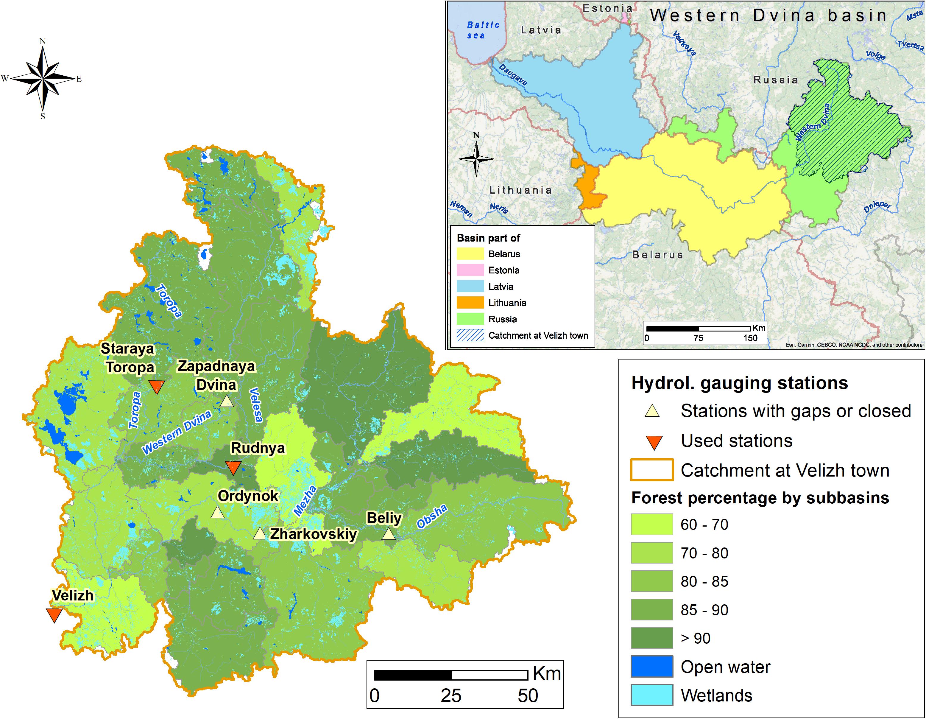
Figure 1. Study area of the Western Dvina catchment (Russian part) with hydrological gaging stations used for model processing.

The Russian part of the Western Dvina river basin is home to approximately 1,70,000 people (8% of the total basin population), of which more than 8300 live in the subbasin’s largest town, Western Dvina (Center for International Earth Science Information Network [CIESIN], 2014) 0.38, 51, and 2% of the total population live in the sub-basins located in Belarus, Latvia and Lithuania live, respectively, of the river basin.

Methods and Data

The hydrological freely accessible model SWAT v.2012 was chosen (Arnold et al., 2012) as a tool to simulate the influence of topography, the influence of soil and LULC on the water balance. The advantages of the SWAT model are the availability of reliable and helpful documentation, the absence of limitations on the catchment area, compatibility with GIS software (ArcGIS, QGIS, MapWindow), the open source computer program for calibration of SWAT models –SWAT Calibration and Uncertainty Programs SWAT-CUP (Abbaspour et al., 2007), and a vast range of scientific publications on different aspects of the model and its practical application. The modeling process of different types of fluxes (water, dissolved and suspended matter) is based on calculations of the river discharge and its parametrization. Setting up a process-based model consisted of several steps: (a) preparation of the input data, including meteorological datasets and catchment layers, (b) optimization of the model (testing model sensitivity to different methods of stream delineation and determining hydrological response units), (c) parameter sensitivity analysis, (d) calibration and validation, and finally, and (e) water balance assessments (Figure 2).

FIGURE 2

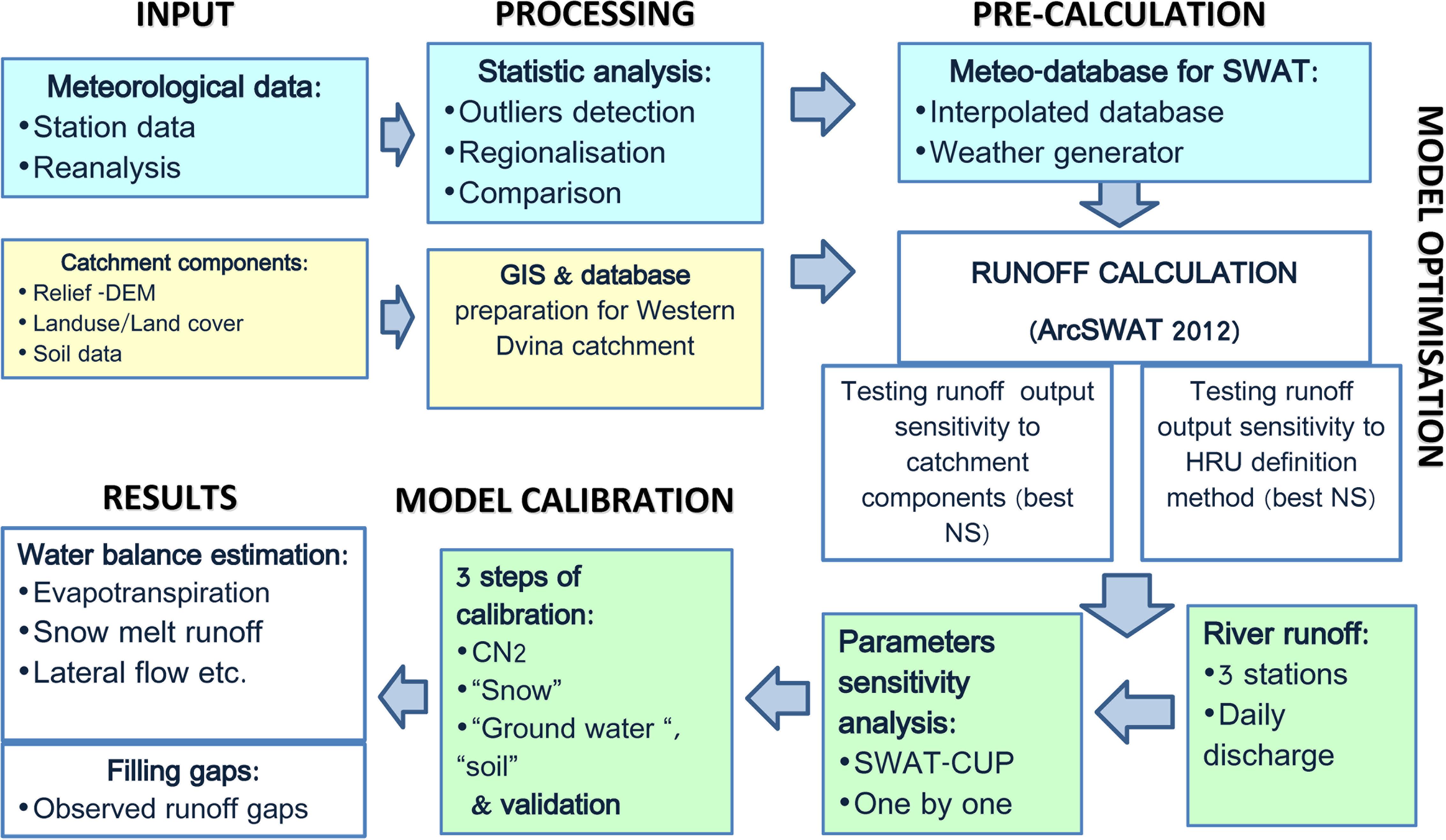
Figure 2. The conceptual framework of the study: water balance model flow of Western Dvina catchment.

Because of gaps in the time series of daily discharge, the period 1989–2004 was chosen for set-up, calibration and validation of the model (Table 1). This period contains years which are representative for relatively wet and dry conditions and can be used for both model calibration and validation. The analysis of data from the Velizh gaging stations revealed a negative runoff trend. Comparing the periods of 1992–2015 and 1976–1991, the average runoff in Velizh decreased (4.66 versus 5.68 km³/year).

TABLE 1

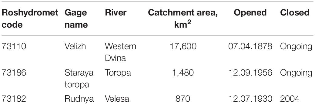
Table 1. Discharge gaging stations situated in the catchment used for model setup, calibration and validation.

Climatic Data Analysis

The SWAT model calculates water balance components using daily minimum (TN) and maximum (TX) air temperatures, precipitations (RR), relative humidity (HU), wind speed (WND), and surface solar radiation downward (SSRD).

The question, which source of meteorological information is most suited for the model is considered in this section. There are several archives containing climate information, which can be divided into observational point and reanalysis data.

Reanalysis a systematic approach to produce global data sets of consistent spatial and temporal resolution. The essence of reanalysis is as follows: observation data are assimilated into a numerical climate model to obtain three-dimensional fields of various atmospheric variables as results. According to Serreze et al. (2005) and (Reichler and Kim, 2008), reanalysis does fairly well regarding temperatures but tends to be more error-prone regarding precipitation. In many reanalysis projects, observed precipitation is not assimilated. It is simulated by the model and shows henceforth more uncertainty. At the same time, the data from meteorological stations are not always accessible or complete, and often contain outliers which require further corrections (e.g., plausibility analyses). In this paper, two databases of the daily meteorological data for the period 1981–2016 were prepared. The first one bases on ECMWF ERA-Interim reanalysis data¹ at its highest resolution of 0.75° × 0.75°, which is equivalent to 84 × 84 km at the equator or 84 × 42 km at 60° north (Berezowski et al., 2016). The second one comprises two meteorological station data sources:

• European Climate Assessment & Data (ECA&D) (Internet Database ECA&D, 2013);

• Global Surface Summary of the Day from the National Climatic Data Center (GSOD NCDC/NOAA) (National Oceanic and Atmospheric Administration, 2019).

For the Russian part of the catchment area, the number of stations inside and outside the catchment area is the same for ECA&D and GSOD NCDC/NOAA databases and equals16. However, not all of these stations are the same. The list of stations considered in the region, with the series length corresponding to the precipitation measurement, is given in Table 2.

TABLE 2

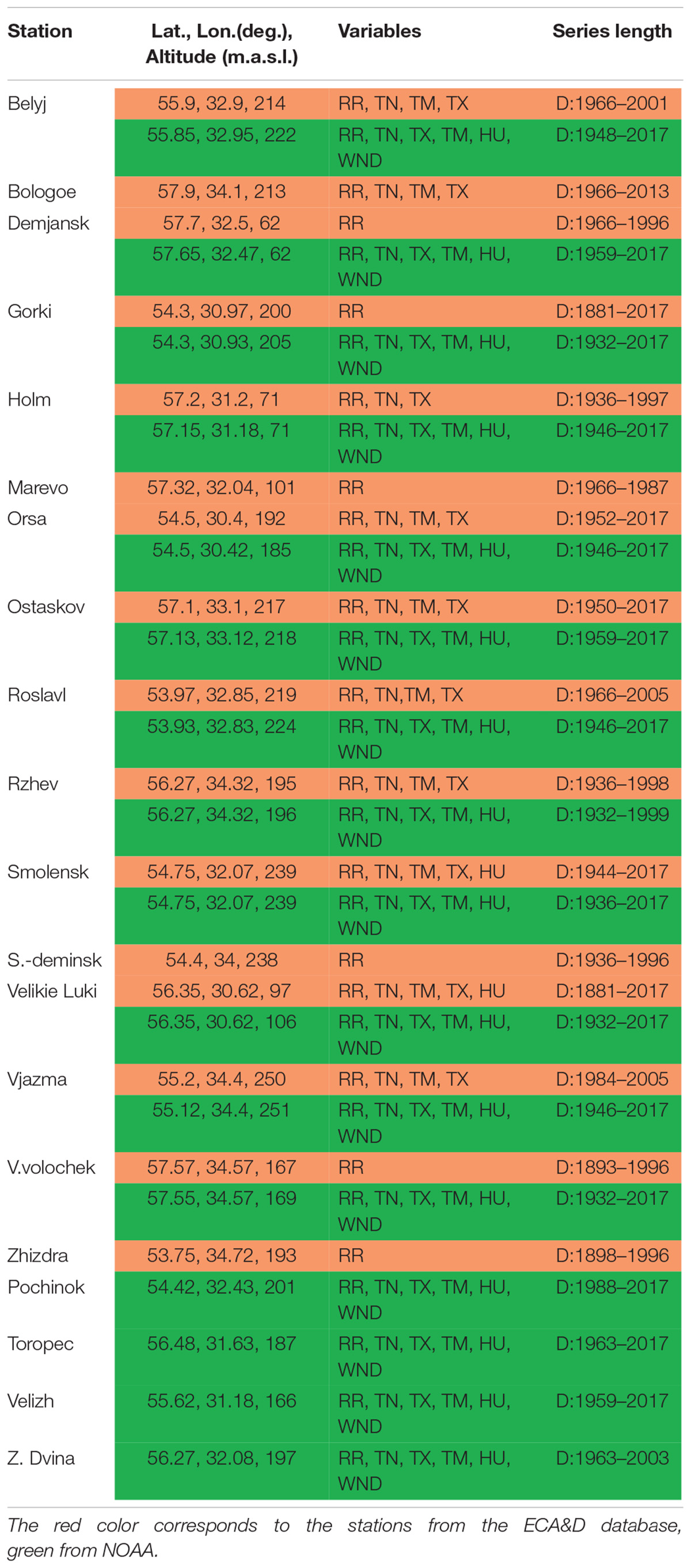
Table 2. Meteorological stations of the investigation area (Russian part of Western Dvina catchment).

In the study area, solar radiation and sunshine duration are not measured; however, these solar characteristics are important for building a future model. Based on the recommendations of the ERA-Interim developers (Dee et al., 2011), the use of sunshine duration is not recommended. Therefore, in the present work, the reanalysis data of Solar Surface Radiation Downward (SSRD) without comparison with the interpolated station data is used.

The location of stations from Table 2 is shown in Figure 3.

FIGURE 3

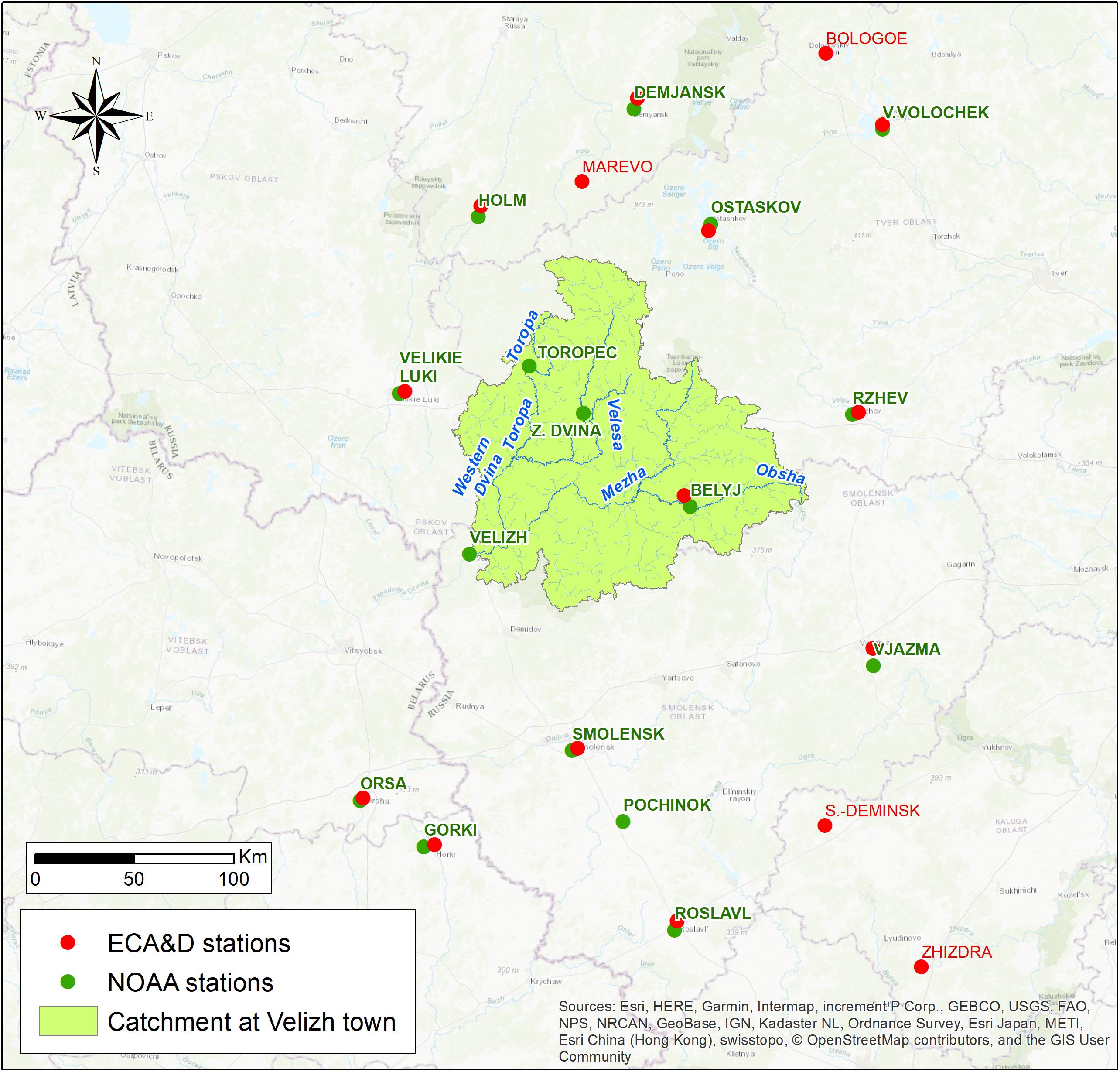
Figure 3. Investigation area (Russian part of Western Dvina catchment). The red color corresponds to the stations from the ECA&D database, green from NOAA.

Plausibility Analysis

Before the data from the stations become publicly available, all values of the variables have already passed a first quality control (Berezowski et al., 2016). However, these first quality checks may not identify all problematic values. Therefore additional outlier tests should be applied.

In meteorology, it is difficult to accurately distinguish between outliers and extreme values. Special attention, especially for highly variable precipitation values is needed. The plausibility analysis consists of four steps: (a) visual inspection, (b) outlier tests, (c) calculation of reference values (RV), and (d) filling in data gaps and replacing suspicious values with RV.

Visual inspection allows determining some implausible values. For example, visualization of precipitation data sets in the GSCD NCDC/NOAA database showed that for most stations precipitation values of 74.9, 150.1, and 300 mm/day were frequently contained in the dataset. Since these values do not correspond to the values for the ECA&D database, these values do not have a logical explanation and seem to indicate a systematic error in the database. These numbers were excluded from further considerations.

Outlier tests of normally distributed values, such as temperature, can be based on three standard deviations method. However, for skewed data, such as precipitation, robust statistics methods such as Median Absolute Deviations (MAD) or Interquartile Range (IQR) should be used (Leys et al., 2013).

It was decided to use the MAD method, which, on the one hand, is sufficiently reliable, on the other hand very simple and universal (Formula 1).

$$\mathrm{Outlier}\mathrm{limits}\text{=}\mathrm{med}(\mathrm{monthly})\pm \mathrm{MADfactor}\cdot \mathrm{MAD} (\mathrm{monthlydata})(1)$$

Outlier limits detection is performed with monthly thresholds for precipitation, temperature, relative humidity; and with seasonal thresholds (3 month) for WND as this parameter is much less time-dependent.

Separate calculations for precipitation thresholds were conducted for stations located between altitudes of 0 to 100 m above mean sea level, and for 100 to 200 m, and 200 m and above.

For precipitation and WND, three MAD factors were selected: 2.5, 3, 3.5, and 4. For temperatures MAD factors were selected within the range 2.5–6.0. For the relative humidity, the limits were set within a range from 0% to 100%.

By comparing the median values of outlier limits depending on different MAD coefficients with actual meteorological data, the value of the MAD coefficient was chosen, according to which the final outlier limits were selected. Values outside the limits determined for each station, depending on the altitude above sea level, were marked as possible outliers.

For this purpose the normal ratio method (Young, 1992) was applied for the reference values (RVs) calculation to determine the set of correlation coefficients between the considered station datasets and each available surrounding station. Correlation coefficients between the 30 nearest meteorological stations were considered.

The following specific analyses were done for each meteorological variable. For precipitation, outliers are identified when the following criteria are fulfilled:

• The outlier test indicates an outlier,

• For small precipitation events (RF < 2 mm): RR/RF > 20,

• For winter precipitation events (RF ≥ 2 mm): RR/RF 8.

For temperature, mean and maximum values, are considered as an outlier if:

• The outlier test indicates an outlier,

• |T – Threshold| ≧ 3°C,

• |T – RV| ≧ 4°C.

For WND, outliers were identified on one of the following criteria:

• The statistical test described above defined it,

• WND – RV > 7 m/s.

The plausibility analysis ends with the replacement of the outlier values by RVs. Finally, the ECA&D and GSOD NCDC/NOAA databases were combined. If the station time series of both databases are highly correlated, the values were directly used to fill the gaps. If there are no values available in both databases, RVs were used.

Regionalization of the Station Data

The main problem when comparing reanalysis data and observed station data is their spatial inconsistency. Measurements at meteorological stations represent a point, while reanalysis data represent average values of the applied spatial grid, which in our case has a spatial resolution of 0.75° × 0.75°.

There are two general approaches to compare station with gridded data: (1) to interpolate the gridded values to the observation points (area-to-point) and (2) to interpolate the point observations onto the reanalysis grid (point-to area). An evaluation of the methods is typically performed with statistical scores such as bias and RMSE.

It should be noted that both methods have considerable drawbacks (Tustison et al., 2001). The magnitude of the representativeness error in each method is significant, and the magnitude of the error in both cases is based primarily on the grid resolution.

Finally the point-to-area method was chosen, since it is widely used in climatological studies and well accepted (Maraun et al., 2010).

To improve the accuracy of the interpolation, the geostatistical spatial pattern analysis method (Christensen, 1991) was used. Many meteorological variables show elevation-dependent gradients. For instance, temperature is mostly decreasing and precipitation increasing with altitude. Therefore, a linear regression model is set up, which considers the dependence of measured values on the altitude of the stations. This model is applied for the whole grid, for which the altitude is known. In a second step, the residuals of each point observation from the linear model were determined. These residuals were interpolated with the inverse distance weighing (IDW) method onto the grid. The sum of the regression and IDW output gave the final value for each cell. Since the values at the boundaries of the considered region are not considered as reliable, it was decided to delete all the values obtained for the boundary beyond the catchment area.

Performance Measures

For comparison of the reanalysis with interpolated station data, a set of performance measures were calculated: root-mean-square error (RMSE), ratio of standard deviations (rSD), index of agreement (d), Pearson correlation coefficient (r), and the bias (BIAS) (Formulas 2 – 6).

The index of agreement is one of the most reliable measures of prediction error (Willmott et al., 2012). This index varies between zero and one (whereby one indicates an ideal agreement). The index of agreement can detect additive and proportional differences in compared pairs in datasets.

Modeling Approach and Spatial Data Description

The catchment model was built with the ArcSWAT2012 GIS-interface. The modeling process of different types of fluxes (water, dissolved and suspended matter) is based on the calculations of river discharge and its parameterization. Modeling with SWAT comprises the following steps: catchment model building (relief data is based on Advanced Land Observing Satelite [ALOS], 2017) including initial soil and plant data (GlobalLand30, 2014) (because no detailed information was available for this study, default parameters were chosen based on global LULC and soil parameters), preparation of the meteorological data, calibration of parameters, validation and then implementation.

The following input data were used (Table 3). Periods of model calibration (1992–1998) and validation (1999–2004) are chosen according to continuous hydrological observations inside the catchment.

TABLE 3

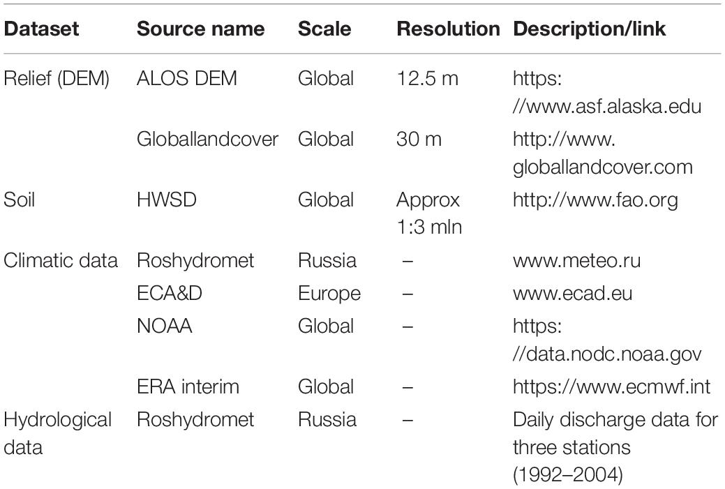
Table 3. The datasets used to set up and operate the model.

It must be noted that for the soils of the catchment HWSD (Harmonized world soil database) (Nachtergaele et al., 2008) contains the characteristics only for two upper soil layers. For this reason, the third and further soil layers were not taken into account in the model.

For the evapotranspiration the Pennman–Monteith approach was chosen, and for the channel routing the Muskingum approach. A period of 3 years was chosen as a spin-up period. To model the rainfall-runoff-routing processes, in this study the Daily rain/CN/daily route method was selected (where CN is a rainfall-runoff curve number) as a default option used by SWAT model (another option is the sub-daily scale). These options are described in Neitsch et al. (2005). The model performance is evaluated with Nash-Sutcliff Efficiency (NS), as main objective function, and Kling-Gupta Efficiency (KGE), square correlation (R2) and PBIAS as additional model performance criteria (Nash and Sutcliffe, 1970; Gupta et al., 1999).

Basins in which a significant part of the runoff is formed by snowmelt tend to be challenging for hydrological models. Freezing and thawing processes modify the flow paths for water and its availability for evaporation (Woo et al., 2000; Hülsmann et al., 2015). In SWAT, hydrological processes including snowmelt are realized at the “hydrological response units” (HRU) level. The watershed is automatically subdivided into a number of subbasins based on provided river network layer and elevation data. In our case, two subbasins were delineated based on manually positioned outlets at discharge gaging sites to include these subbasins into calibration procedure using measured time series. The last subbasin is terminates at the outlet of whole catchment at the gaging station Velizh. Portions of a subbasin that possess unique land use/management/soil attributes are grouped together and defined as one HRU (Neitsch et al., 2005). Depending on Data Availability and modeling accuracy, one subbasin may have one or several HRUs defined.

Preliminary results of the discharge model allowed us to identify the best method for determining HRUs. For the delineation of the “hydrological response units” (HRU) threshold values of 20/10/20 percent for land cover, soil and slope areas were chosen, respectively, because this percentage brings the best NS value for preliminary modeling results without calibration procedure. NS was also chosen as the objective function for model calibration.

Parameter sensitivity analysis was performed manually using the software SWAT-CUP (one by one to determine the effect of each parameter on the result. Nineteen sensitive parameters were found to be sensitive. They were divided into genetically homogeneous groups: CN2 parameter (runoff curve number), “snow” parameters, “soil and groundwater” parameters, other parameters.

When the mean daily air temperature is less than the snowfall temperature, the precipitation within an HRU is classified as snow and the liquid water equivalent of the snow precipitation is added to the snowpack. The snowpack increases with additional snowfall, but decreases with snowmelt or sublimation. The SWAT model has eight “snow” parameters directly related to snow water equivalent calculations and freezing-melting processes: SFTMP (snow fall temperature), SMTMP (snow melt base temperature), SMFMX (maximum melt rate), SMFMN (minimum melt rate), SNOCOVMX (snow water equivalent before melting), SNO50COV (fraction of snow cover), TIMP (snow pack temperature lag time) and CN_FROZ (parameter for frozen soil adjustment). Main “soil and groundwater” parameters include SOL_AWC (available water capacity), ALPHA_BF (base flow factor), GW_DELAY (groundwater delay), RCHRG_DP (Deep aquifer percolation fraction), ESCO (evaporation compensation factor) and others (Neitsch et al., 2005).

Calibration and Validation

It is recommended that the calibration and validation periods should include a comparable number of dry, medium, and wet years (Arnold et al., 2012). Based on the analysis of the residual mass curve of annual runoff, the period 1989–2004 (including 3 years of “spin-up”) is considered as the average period. Both series – calibration and validation contain dry (1997, 2002) and wet (1995, 1999) years. The model was calibrated and validated using daily discharge time series for three gaging stations inside the basin all together by adjusting the best objective function value for each gauge.

As the first step, “snow” parameters were calibrated inside the physically based range with automatic procedure (SWAT-CUP) separately from the other groups of parameters. Values for snow water equivalent before melting (SNOCOVMX) and initial temperature of snow fall and snowmelt (SFTMP, SMTMP) with very small parameters range were defined for fine tuning during the further calibration procedure. To put the SNOCOVMX in realistic range, nearest station data was used. For the stations Velikie Luki and Velizh maximum decadal snow water equivalent falls in range 60–110 mm. In a second step, CN2 parameter was set for forested and non-forested land cover types and calibrated as a distributed parameter together with “snow” parameters small range. This small range was defined on the previous step and this range has not been changed during the whole calibration procedure.

In a third step, genetically homogeneous parameters (ground water and soil routine parameters) and other sensitive parameters (e.g., evapotranspiration rate and channel routing) were calibrated within physically based ranges with the autocalibration procedure SUFI-2, which is provided by the SWAT-CUP software.

Results

Climatic Components Analysis

The meteorological station data were processed for elimination of outliers and interpolated into the selected grid, taking into account the altitude of each cell above sea level. Furthermore, these two data sets (reanalysis and interpolated station data) were compared with each other using the methods of descriptive statistics. The demonstrated difference between the datasets shows that the reanalysis and interpolated stations data results are very similar to each other. This is evidenced by similar seasonal and climate change trends and significant spatial correlation coefficients between datasets. The results are summarized in Table 4.

TABLE 4

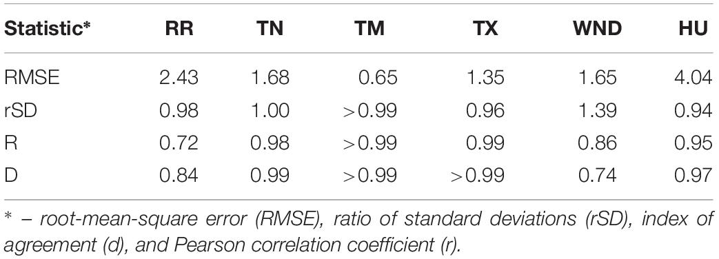
Table 4. Descriptive statistical analysis for the meteorological variables comparing reanalysis and interpolated station data: precipitation (RR), mean temperature (TM), wind speed (WND), and relative humidity (HU).

The correlation coefficients are significant everywhere (r > 0.72). The values of temperatures correlate very well with each other. Despite the high correlation coefficient (r > 0.86) the WND time series do not agree well with each other (d = 0.74), due to some difference in the amplitude of the values (difference of 1.38 m/s or 33%). One of the possible reasons for this is an underestimation of the surface roughness for the particular region in the reanalysis.

Meteorological variables have a pronounced seasonal distribution. The interpolated stations data and reanalysis graphs repeat each other quite well throughout the year (Figure 4), with the exception of WND.

FIGURE 4

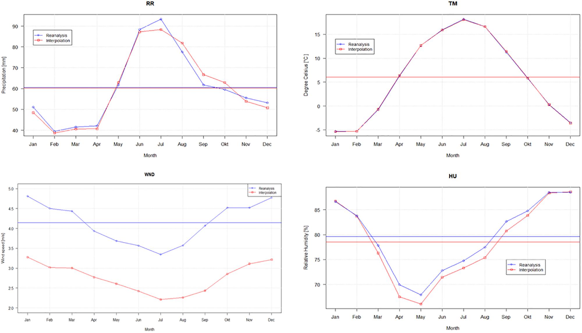
Figure 4. Seasonal cycles of interpolated stations and reanalysis ECMWF ERA-Interim data for precipitation (RR), mean temperature (TM), wind speed (WND), and relative humidity (HU).

The annual precipitation for the interpolated station data and the reanalysis is 723 and 725 mm, respectively. According to Timm et al. (2009), the average annual precipitation for the entire Western Dvina catchment area ranges from 600 to 800 mm, which corresponds to the data obtained.

The reanalysis and interpolated stations data curves of the mean temperatures are very similar. Interestingly, the maximum temperatures of reanalysis show lower and the minimum temperatures show higher values than interpolated station data. This means that temperature regime of the reanalysis is smoothened.

Long-term reanalysis and interpolated stations data curves have the same shape. Gradual increasing trends of temperatures and surface solar radiation are indicators of warming over the past few decades. Trends are very similar for temperature and WND, but differ for precipitation (Figure 5).

FIGURE 5

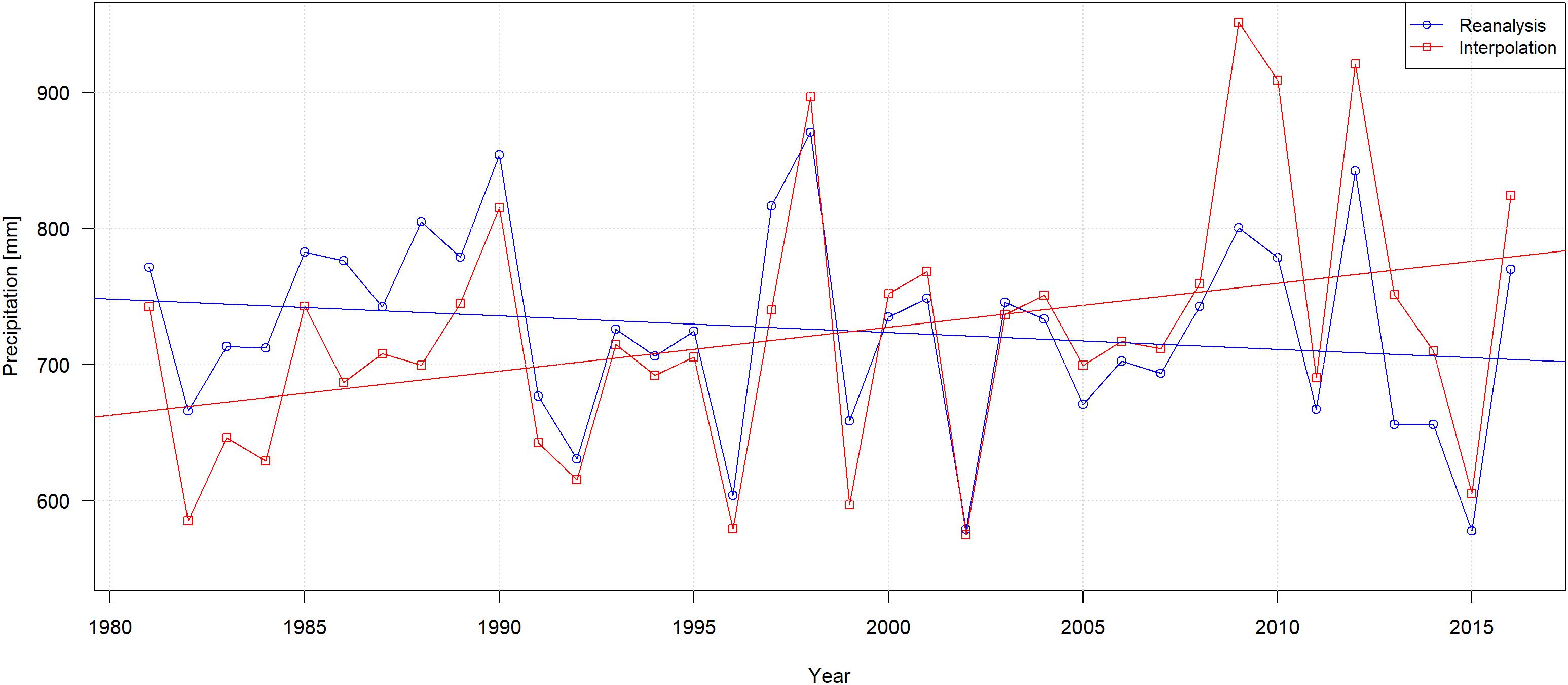
Figure 5. Comparison of annual mean precipitation (RR) obtained by interpolation of station data and reanalysis ECMWF ERA-Interim.

The use of interpolated station data with SSRD from reanalysis is the preferable solution for meteorological input for Western Dvina catchment model. Thus, for the runoff modeling authors have prepared and used the meteorological database filled with the interpolated station data and SSRD component from ECMWF ERA-Interim reanalysis. We have used the five nearest and most reliable meteorological stations – Velizh, Belyi, Toropetz, Velikiye Luki, and Smolensk. These stations have the most complete sets of measured data on all weather parameters. SWAT input datasets were completed by filling gaps with interpolated NOAA/ECA&D station data and with SSRD interpolated from ERA-Interim gridded data into station locations.

SWAT Model Calibration and Validation Results

Initial SWAT-based water balance component calculations (without calibration) for Western Dvina catchment for the period 1992–2004 gave adequate values. Simulated annual runoff is 278 mm (observed is 275 mm), evapotranspiration is 379 mm (395 mm estimated by MODIS – MOD16 Global).

Sensitivity analysis made with one-by-one method (SWAT-CUP) allowed to identify 19 sensitive parameters. Results of parameter calibration are shown in Table 5. According to Moriasi et al. (2007) model efficiency is satisfactory (Table 6).

TABLE 5

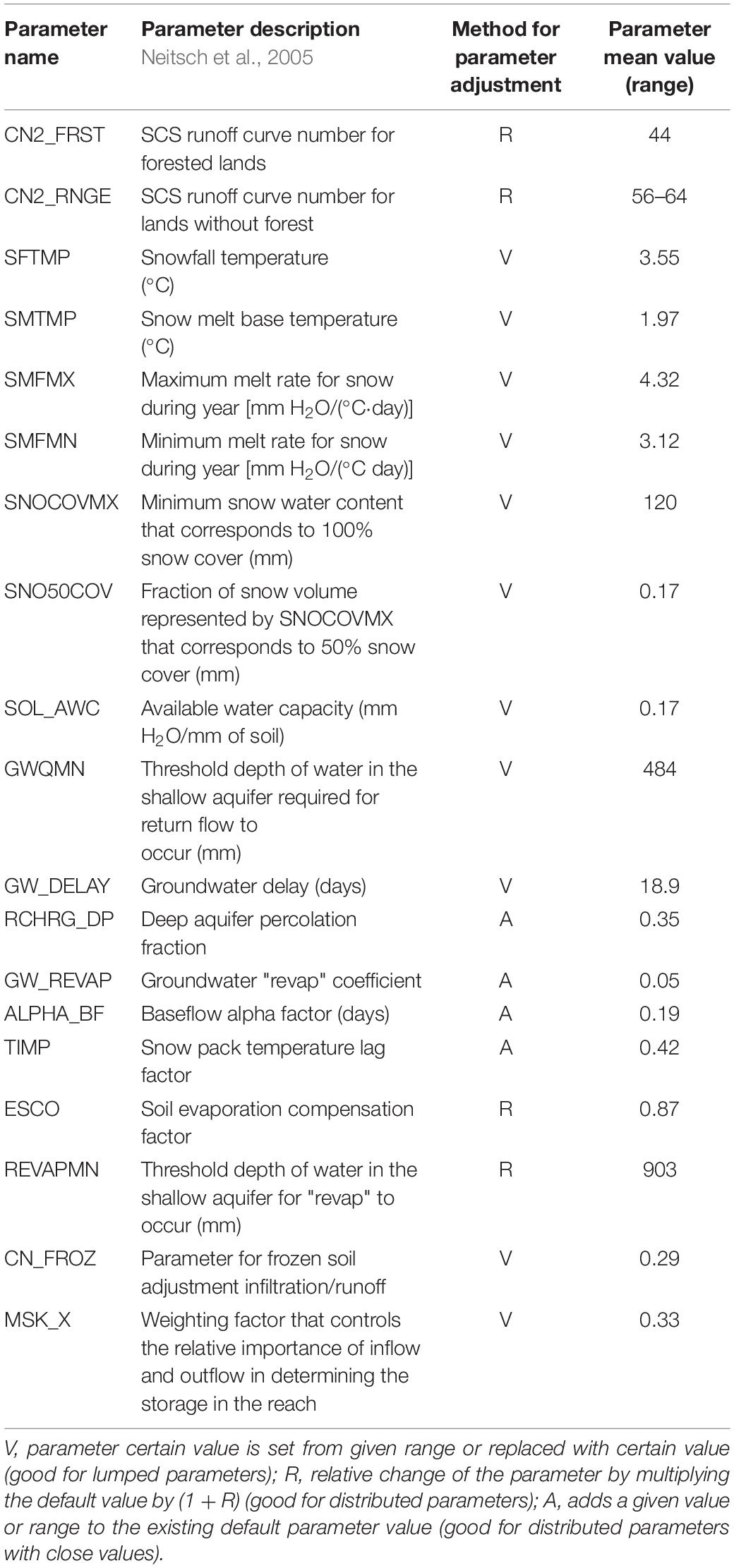
Table 5. Parameters calibration results for the model.

TABLE 6

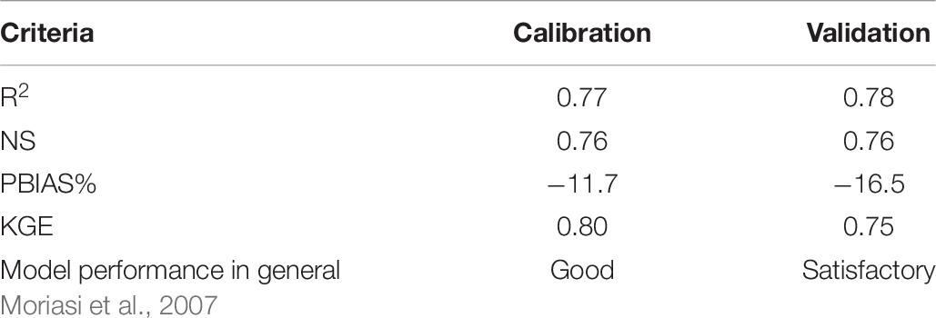
Table 6. Model efficiency evaluation for daily runoff calculation.

The model simulates well the beginning of floods, but peaks are underestimated especially for highest peaks (Figure 6). The recession of the flood curve is simulated too slow.

FIGURE 6

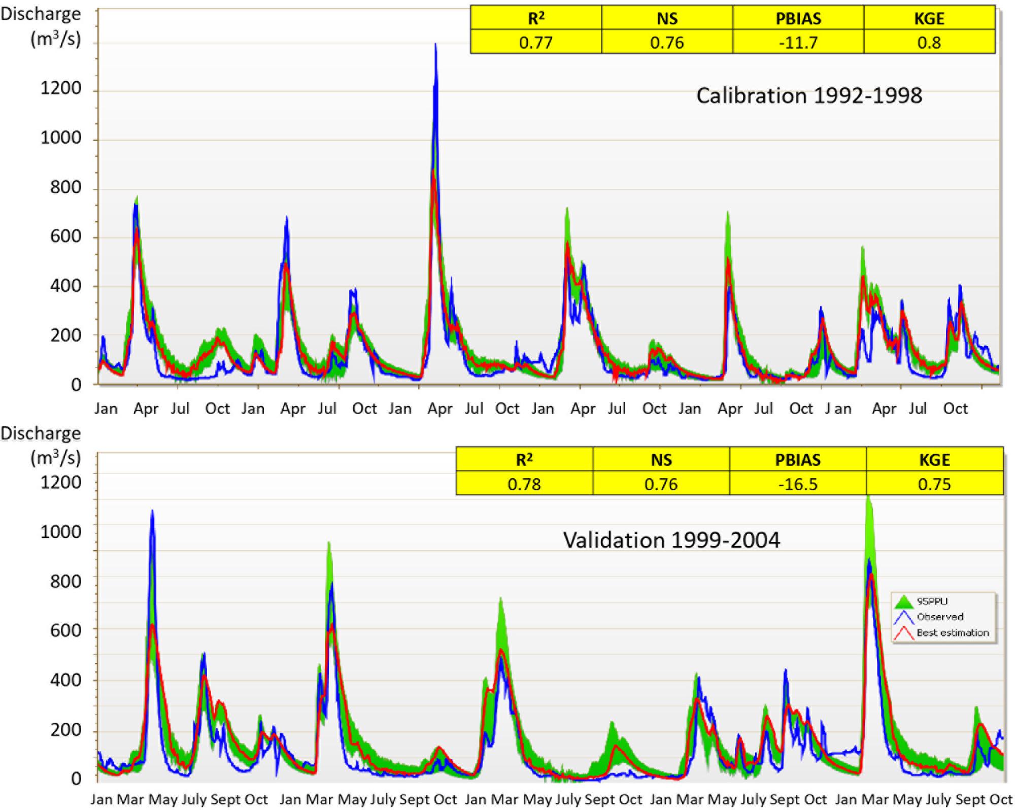
Figure 6. Model calibration and validation. Western Dvina river at Velizh town, blue line represents measured runoff, red line – simulated runoff in cubic meters per second (Q, m³/s), green area – 95 percent prediction uncertainty range (95 PPU).

At the same time it is obvious that small rain floods are often simulated with insufficient accuracy. We consider two reasons. Because of sparse station density, spatial distribution of rainfall is insufficiently captured. Furthermore, the insufficient reproduction of the soil distribution and its parameters can course an erroneous simulation of water flows.

Water Balance Components Calculation

For the period 1992–2016, water balance components were calculated based on simulated annual means. Annual snowmelt water amount is about 20–30% of annual precipitation sum. Mean annual water discharge is overestimated and also minimum and maximum values (Table 7).

TABLE 7

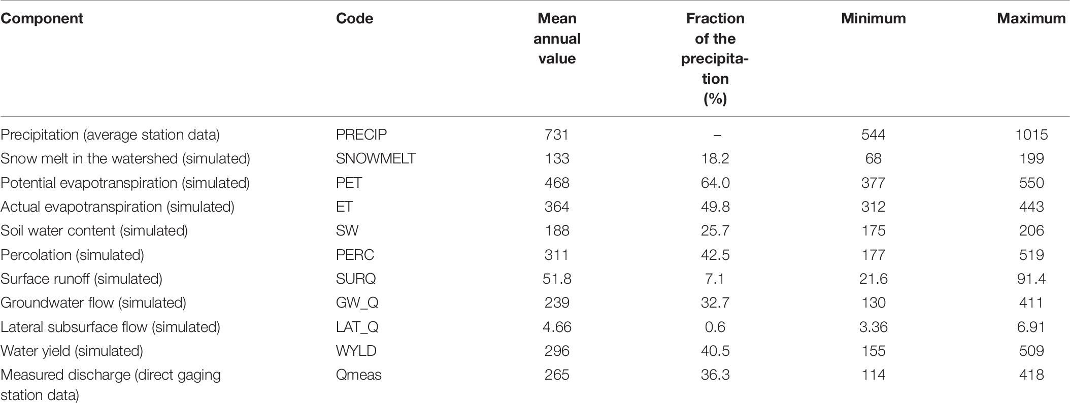
Table 7. Simulated annual water balance components for the period 1992–2016 (values of annual sums in mm) and the fraction of the annual sum of precipitation (%).

Precipitation has the increasing trend, snowmelt does not have trend, runoff and evapotranspiration have also increasing trend (not statistically significant). Snowmelt occurs at the end of the winter and the maximum amount of melted water coincides mostly with maximal runoff (Figure 7).

FIGURE 7

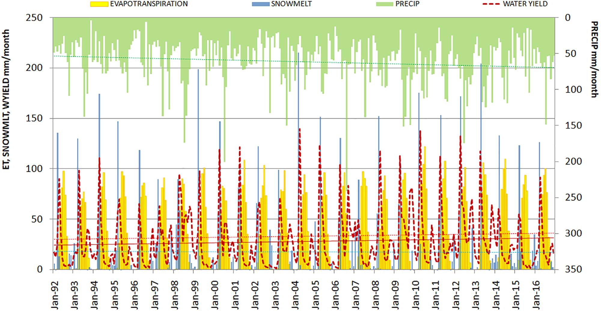
Figure 7. Simulated monthly runoff, snowmelt, evapotranspiration, and measured precipitation sum (reverse scale) for the period of 1992–2016.

Spatial distribution of all simulated water balance components represents the structure of flow generation drivers inside the catchment. It strongly depends on land cover. The highest ET is linked to subbasins with lakes predomination in the western part of the catchment – correlation between open water fraction of each subbasin and ET of each subbasin is 0.78 and it is the highest for certain subbasin which contain largest lakes.

The wetlands fraction varies between 0 and 33% of subbasin area and has the strongest impact on flow generation variability among other main land cover types, with correlations reaching 0.72 and 0.51 for surface runoff and soil water. However, percolation and ground water flow are negatively correlated to the wetlands fraction of the subbasin area (correlation for both is −0.69). Wetlands significantly increase surface runoff by decreasing percolation and ground water yield. Forest coverage in the subbasins ranges between 62% and complete forest cover (100%). It does not have strong affect on water balance fluctuations between subbasins (correlation varies from −0.23 to 0.12).

Higher snowmelt is linked to higher precipitation in the eastern part. In general higher soil water and lower lateral and groundwater flow are linked to gleic soils and histosols widespread in wetlands (Figure 8).

FIGURE 8

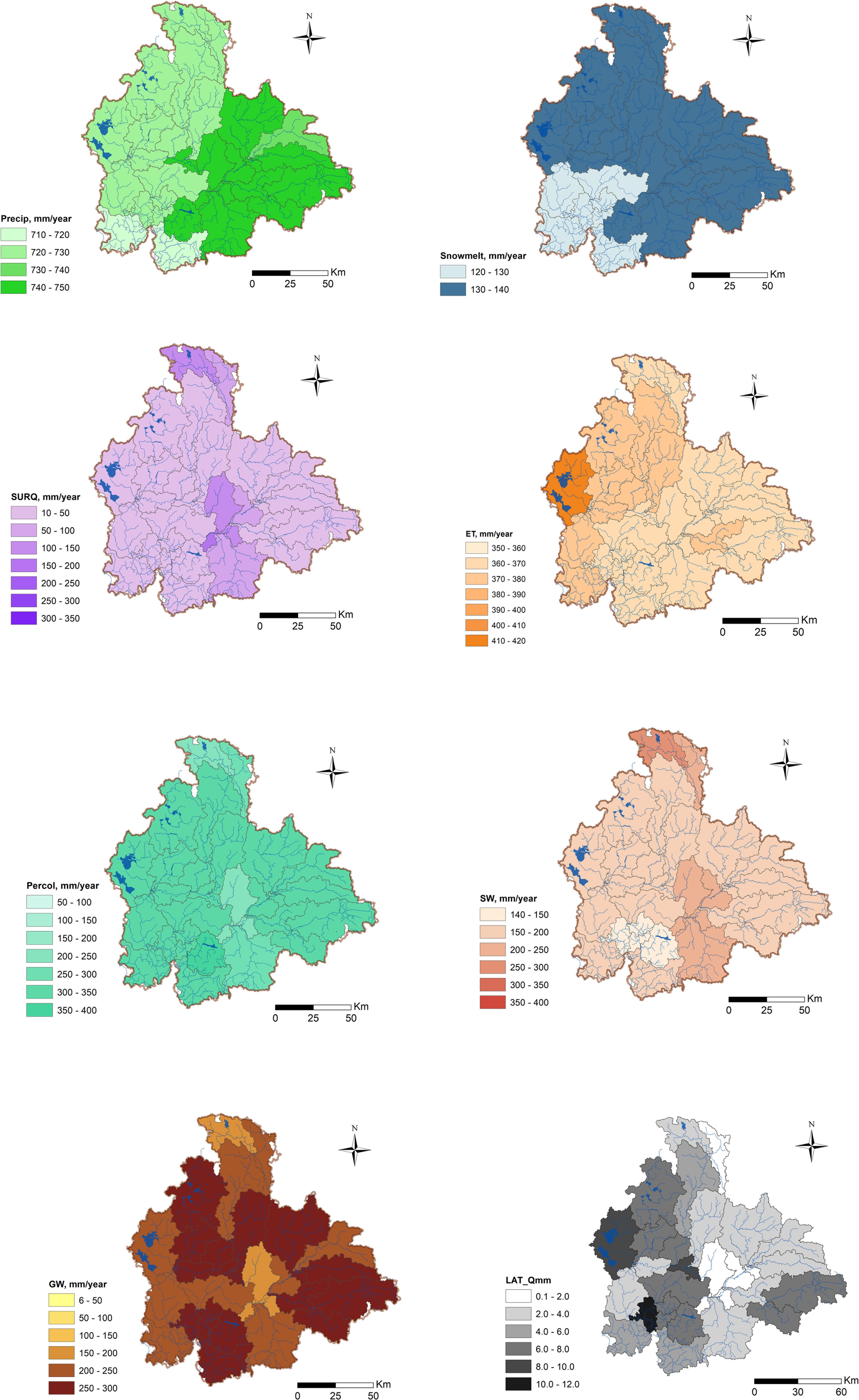
Figure 8. Annual calculated mean water balance components distribution on the Western Dvina catchment area (Precipitation, snowmelt, surface Q, actual ET, percolation, soil water, ground water, and lateral Q).

Discussion

The analysis of climate data from different sources was performed to identify the best input for the hydrological model SWAT. Station data of the ECA&D and the GSOD NCDC/NOAA databases were compared with the reanalysis ECMWF ERA-Interim. The average annual precipitation is almost the same in the two cases under consideration (723 and 725 mm for interpolated station data and reanalysis, respectively). There is a discrepancy between precipitation trends in the period 1981–2016. Reanalysis data show a downward trend whereas interpolated station data does not. Interpolated station data have lower values than reanalysis at the beginning and higher values at the end of the period. The reason for this discrepancy may be the decreasing number of station data over time. One of the trends in the region under consideration is the closure of stations recording comparatively low precipitation sums. Mean temperature values coincide very well, but daily minimum and maximum temperatures are underestimated by the reanalysis.

The relative humidity values of the reanalysis are slightly higher than interpolated station data. The WND values are about 33% (or 1.38 m/s) higher for reanalysis in comparison to interpolated station data.

As there are no observations from the solar energy component at the stations, and since sunshine duration is not recommended to use from reanalysis, the SSRD from reanalysis was the only reasonable choice.

Because of mentioned uncertainties of reanalysis data, it was decided to use station data for precipitation, temperature, humidity and WND.

In general the model shows a “good” performance for river runoff simulation based on rough open source data. But mean runoff is overestimated. One of the reasons is an overestimated (comparing to naturally considered) SNOCOVMX parameter which was obtained by the calibration procedure and provided best representation of hydrograph.

The model overestimates mostly the low flow which can be explained by the general error in evapotranspiration calculation (based on methods without sufficient taking into account the transpiration processes) and insufficient consideration of surface water and ground water interactions, because these two processes are the most important for the summer base flow assessment.

The most sensitive are the “snow” and “groundwater” parameters, and also the distributed CN2 parameter. The calibration of the “snow” parameters should be done separately from others. Moreover, it should be considered that the open source soil database, which was used, included only the two uppermost soil levels.

In general model uncertainties may have several reasons. In Russian Federation gaging network is sparse and has many gaps in data. Global spatial data used for land cover and soil databases does not consider local features – e.g., temporal variability of wetlands conditions, local soil distribution (for example, alluvial soils in river valleys, peat soils).

Also two features of the SWAT model may cause some more uncertainties for this region. First, freezing and thawing of soil water are not considered by the SWAT model. Second – it has lumped snow parameters, which could not be distributed for such flattened catchment and could not be calibrated separately for different land cover types.

Inside the Russian part of Western Dvina catchment the absence of runoff measurement in huge wetlands, which were drained with abandoned drainage channels, creates a strong data deficit for runoff modeling. All possible data sources and field investigations should be taken into account for model improvement, particularly data on soil profile characteristics and snow cover dynamics during the winter and adjacent seasons. Ideally, the soil database should be more detailed.

In comparison to other water balance research papers (e.g., Pluntke et al., 2014; Rouholahnejad Freund et al., 2017; Osypov et al., 2018) it should be noted that SWAT based surface and lateral flow are rather low in most cases. Daily runoff models often are based on specialized local soil maps and LULC databases which may provide adequate ground and lateral flow parameters and their distribution. In most cases SFTMP and SMTMP are close to 0 degrees, but in the spring highly forested lands may store coldness longer than open areas where stations are often situated. In reality, the lumped snowmelt temperature may be higher than suggested by station temperatures of 0°C; for example, it is known that forested area temperatures are about 2 degrees lower for some Russian Far East river basins as compared to station temperatures (Bugaets et al., 2018).

The calibrated model can be implemented to estimate some water balance components in case of climate change in the future. With the input climatic projections data the assessment of the annual distribution dynamics of the evapotranspiration, snow melt, surface, lateral and ground flow can be done for Western Dvina catchment.

Semi-distributed water runoff models can be used as an important part of water resources monitoring strategies and can play a significant role in transboundary water resources management (see Alekseevskii et al., 2015). Moreover, well calibrated models are an important tool for various applications in water management, such as the estimation of water resources availability and balances, water quality and sediment transport modeling etc.

Author Contributions

PT made the proposal, performed the calculations with SWAT model and drafted the manuscript. AK made the climatic analysis, prepared the meteorological database, and wrote parts of the manuscript text. SC is a leader of the Russian team of MANTRA-Rivers project and wrote parts of the manuscript text. AT provided the GIS support and made the editorial work. DK is one of the MANTRA-Rivers project scientists, proofread and improved the manuscript. PB is one of the MANTRA-Rivers project scientists, prepared and processed the input data. TP is the leader of MANTRA-Rivers project from German side and suggested conclusions for the manuscript.

Funding

This study was supported by the Volkswagen Foundation within the project “Management of Transboundary Rivers between Ukraine, Russia and the EU – Identification of Science-Based Goals and Fostering Trilateral Dialogue and Cooperation (ManTra-Rivers)” (Grant No: Az.: 90 426).

Conflict of Interest Statement

The authors declare that the research was conducted in the absence of any commercial or financial relationships that could be construed as a potential conflict of interest.

Acknowledgments

The authors would like to thank the Volkswagen Foundation for the funding provided for the project “Management of Transboundary Rivers between Ukraine, Russia and the EU – Identification of Science-Based Goals and Fostering Trilateral Dialogue and Cooperation (ManTra-Rivers)”. GIS analyses are done within the framework of Russian Scientific Foundation project (18-17-00086). The authors are grateful to all who helped to organize the collaboration: Yu. Nabivanets and N. Osadcha (Hydrometeorological Institute, Ukraine), and C. Bernhofer and B. Helm (Technical University of Dresden, Germany).

Footnotes

1. ^ http://apps.ecmwf.int/datasets/

References

Abbaspour, K. C., Vejdani, M., and Haghighat, S. (2007). “SWAT-CUP calibration and uncertainty programs for SWAT,” in Proceedings of the MODSIM 2007 International Congress on Modelling and Simulation, eds L. Oxley and D. Kulasiri (Canberra, ACT: Modelling and Simulation Society of Australia and New Zealand), 1603–1609.

Google Scholar

Advanced Land Observing Satelite [ALOS] (2017). Dataset: JAXA/METI ALOS-1 PALSAR RTC. Available at: http://www.eorc.jaxa.jp/ALOS/en/obs/palsar_strat.htm (accessed August 15, 2017).

Google Scholar

Alekseevskii, N., Zavadskii, A., Krivushin, M., and Chalov, S. (2015). Hydrological monitoring at international rivers and basin. Water Resour. 42, 747–757. doi: 10.1134/s0097807815060020

CrossRef Full Text | Google Scholar

Arnold, J. G., Moriasi, D. N., Gassman, P. W., Abbaspour, K. C., White, M. J., Srinivasan, R., et al. (2012). SWAT: model use, calibration, and validation. Trans. ASABE 55, 1491–1508. doi: 10.13031/2013.42256

CrossRef Full Text | Google Scholar

Asadchaya, M., and Kolmakova, Y. (2014). Tendencies of changes of Belarusian rivers water flow in years of minimum and maximum water availability in climate warming conditions. Bull. Belarusian State Univ. Ser. 2, 84–88.

Google Scholar

Berezowski, T., Szczesniak, M., Kardel, I., Michalowski, R., Okruszko, T., Mezghani, P., et al. (2016). High-resolution gridded daily precipitation and temperature data set for two largest Polish river basins. Earth. Syst. Sci. Data 8, 127–139. doi: 10.5194/essd-8-127-2016

CrossRef Full Text | Google Scholar

Bugaets, A. N., Gartsman, B. I., Tereshkina, A. A., Gonchukov, L. V., Bugaets, N. D., Sidorenko, N., et al. (2018). Using the SWAT model for studying the hydrological regime of a small river basin (the Komarovka River, Primorsky Krai). Russian Meteorol. Hydrol. 43, 323–331. doi: 10.3103/s1068373918050060

CrossRef Full Text | Google Scholar

Center for International Earth Science Information Network [CIESIN] (2014). Columbia University.Gridded Population of the World, Version 4 (GPWv4) 2014. Palisades, NY: Columbia University.

Google Scholar

Christensen, R. (1991). Linear Models for Multivariate, TimeSeries, and SpatialData. New York, NY: Springer.

Google Scholar

Dee, D., Uppala, S., Simmons, A., Berrisford, P., Poli, P., Kobayashibi, S., et al. (2011). The ERA-Interim reanalysis: configuration and performance of the data assimilation system. Q. J. R. Meteor. Soc. 137, 553–597.

Google Scholar

GlobalLand30 (2014). Open source data “30-meter GlobalLand Cover Data Product”, 2014. Available at: http://www.globallandcover.com/ (accessed November 19, 2017).

Google Scholar

Gupta, H. V., Sorooshian, S., and Yapo, P. O. (1999). Status of automatic calibration for hydrologic models: comparison with multilevel expert calibration. J.Hydrolog. Eng. 4, 135–143. doi: 10.1061/(ASCE)1084-069919994:2(135)

CrossRef Full Text | Google Scholar

Heininen, L. (2018). Arctic geopolitics from classical to critical approach – importance of immaterial factors. Geography. Environ. Sustain. 11, 171–186. doi: 10.24057/2071-9388-2018-11-1-171-186

CrossRef Full Text | Google Scholar

Hülsmann, L., Geyer, T., Schweitzer, C., Priess, J., and Karthe, D. (2015). The effect of subarctic conditions on water resources: initialresults and limitations of the SWAT model applied to the KharaaRiver Basin in Northern Mongolia. Environ. Earth Sci. 73, 581–592. doi: 10.1007/s12665-014-3173-1

CrossRef Full Text | Google Scholar

Internet Database ECA&D (2013). European Climate Support Network of EUMETNET Report 2008. Available at: www.ecad.eu/

Google Scholar

Karthe, D., Chalov, S., and Borchardt, D. (2015). Water resources and their management in central asia in the early 21st century: status, challenges and future prospects. Environ. Earth Sci. 73, 487–499. doi: 10.1007/s12665-014-3789-1

CrossRef Full Text | Google Scholar

Krengel, F., Bernhofer, C., Chalov, S., Efimov, V., Efimova, L., Gorbachova, L., et al. (2018). Challenges for transboundary river management in Eastern Europe–three case studies. J. Geogr. Soc. Berlin 149, 157–172.

Google Scholar

Leys, C., Ley, C., Klein, O., Bernard, P., and Licata, L. (2013). Detecting outliers: do not use standard deviation around the mean, use absolute deviation around the median. J. Exp. Soc. Psychol. 49, 764–766. doi: 10.1016/j.jesp.2013.03.013

CrossRef Full Text | Google Scholar

Loginov, V., Volchek, A., and Shelest, T. (2015). Analysis and modeling of hydrographs of rain floods on Belarusian rivers. Water Resour. 42, 292–301. doi: 10.1134/s0097807815030069

CrossRef Full Text | Google Scholar

Maraun, D., Wetterhall, F., Ireson, A. M., Chandler, R. E., Kendon, E. J., Widmann, M., et al. (2010). Precipitation downscaling under climate change: recent developments to bridge the gap between dynamical models and the end user. Rev. Geophys. 48, 1–34.

Google Scholar

Mohrholz, V. (2018). Major baltic inflow statistics – revised. Front. Mar. Sci. 5:384. doi: 10.3389/fmars.2018.00384

CrossRef Full Text | Google Scholar

Moriasi, D. N., Arnold, J. G., Van Liew, M. W., Bingner, R. L., Harme, R. D., and Veith, T. L. (2007). Model evaluation guidelines for systematic quantification of accuracy in watershed simulations. Am. Soc. Agric. Biol. Eng. 50, 885–900. doi: 10.13031/2013.23153

CrossRef Full Text | Google Scholar

Nachtergaele, F., Van Velthuizen, H., Verelst, L., Batjes, N., Dijkshoorn, K., Van Engelen, V., et al. (2008). Harmonized World Soil Database. Rome: Food and Agriculture Organization.

Google Scholar

Nash, J. E., and Sutcliffe, J. V. (1970). River flow forecasting through conceptual models I. A discussion of principles. J. Hydrol. 10, 282–290. doi: 10.1016/0022-1694(70)90255-6

CrossRef Full Text | Google Scholar

National Oceanic and Atmospheric Administration (2019). Global Surface Summary of the Day – GSOD. Available at: https://data.nodc.noaa.gov/cgi-bin/iso?id=gov.noaa.ncdc:C00516 (accessed June 12, 2019).

Google Scholar

Neitsch, S. L., Arnold, J. G., Kiniry, J. R., and Williams, J. R. (2005). Soil and Water Assessment Tool.Theoretical Documentation. Version 2005. Berlin: Springer.

Google Scholar

Osypov, V., Osadcha, N., Hlotka, D., Osadchyi, V., Nabyvanets, J. (2018). The desna river daily multi-site streamflow modeling using SWAT with detail snowmelt adjustment. J. Geogr. Geol. 10, 92–110.

Google Scholar

Parfomuk, S. (2006). Analysis of perennial fluctuations in the annual water flow of the Western Dvina River. Bull. Polotsk State Univ. Ser. B Appl. Sci. 3, 178–182.

Google Scholar

Pluntke, T., Pavlik, D., and Bernhofer, C. (2014). Reducing uncertainty in hydrological modelling in a data sparse region. Environ. Earth Sci. 72, 4801–4816. doi: 10.1007/s12665-014-3252-3

CrossRef Full Text | Google Scholar

Reichler, T., and Kim, J. (2008). Uncertainties in the climate mean state of global observations, reanalyses, and the GFDL climate model. J. Geophys. Res. 113:D05106. doi: 10.1029/2007JD009278

CrossRef Full Text | Google Scholar

Rouholahnejad Freund, E., Abbaspour, K. C., and Lehmann, A. (2017). Water resources of the Black Sea catchment under future climate and landuse change projections. Water 9:598. doi: 10.3390/w9080598

CrossRef Full Text | Google Scholar

Serreze, M., Barrett, A., and Lo, F. (2005). Northern high-latitude precipitation as depicted by atmospheric reanalyses and satellite retrievals. Mon. Weather Rev. 133, 3407–3430. doi: 10.1175/mwr3047.1

CrossRef Full Text | Google Scholar

Volchek, A., and Lusha, V. (2006). Cyclicity of the annual flow of the Western Dvina. Bull. Polotsk State Univ. 3, 172–177.

Google Scholar

Volchek, A., and Shelest, T. (2012). Winter floods forming on Belarusian rivers. Saint-Petersburg: Uchenye zapiski Rossiyskogo gosudarstvennogo gidrometeorologicheskogo universiteta, 5–19.

Google Scholar

Timm, H., Olsauskyte, V., and Druvietis, I. (2009). “Rivers of Europe,” in Baltic and Eastern Continental Rivers, eds K. U. Tockner and C. T. Uehlinger (London: Academic Press), 607–642.

Google Scholar

Tustison, B., Harris, D., and Foufoula-Georgiou, E. (2001). Scale issues in verification of precipitation forecasts. J.Geophys. Res. Atmos. 106, 11775–11784. doi: 10.1029/2001jd900066

CrossRef Full Text | Google Scholar

Willmott, C. J., Robeson, S. M., and Matsuura, K. (2012). A refined index of model performance. Int. J. Climatol. 32, 2088–2094. doi: 10.1002/joc.2419

CrossRef Full Text | Google Scholar

Woo, M. K., Marsh, P., and Pomeroy, J. W. (2000). Snow, frozen soils and permafrost hydrology in Canada, 1995–1998. Hydrol. Process. 14, 1591–1611. doi: 10.1002/1099-1085(20000630)14:9<1591::aid-hyp78>3.3.co;2-n

CrossRef Full Text | Google Scholar

Young, K. (1992). Three-way Model for interpolating for monthly precipitation values. Am. Meteorol. Soc. 120, 2561–2569. doi: 10.1175/1520-0493(1992)120<2561:atwmfi>2.0.co;2

CrossRef Full Text | Google Scholar