Sea Level Trends and Variability of the Baltic Sea From 2D Statistical Reconstruction and Altimetry

Introduction

Considering ongoing climate change, adequate quantification of the global pattern of sea level change is of crucial importance to helping societies cope with its adverse impact on the future (IPCC, 2013). As the sea surface topography may dynamically vary in time and space in intricate patterns, the impact of climate change and of sea level change also occur differently in various areas on Earth (Milne et al., 2009). This is particularly true for the semi-enclosed seas like the Baltic Sea (Hünicke et al., 2015; Suursaar and Kall, 2018).

Sea level measurement history in the Baltic Sea extends back to the 1770s, when tide gauge in Stockholm became operational (Ekman, 1996). Nevertheless, a problem in quantification of general sea level trends is that traditional, tide gauge-based estimation of relative sea level (RSL) change is dependent on local, spatially varying land surface movements (Santamaría-Gómez et al., 2017). Their removal, on the other hand, requires the use of a truly fixed (geocentric) reference network. Finally, tide gauges are mostly coastal-bound and unevenly spaced, and thus, not entirely representative for the whole sea area (e.g., Woodworth, 2006). Recent development in Global Isostatic Adjustment (GIA) modeling (e.g., Spada, 2017; Simon et al., 2018; Vestøl et al., 2019), use of satellite altimetry (e.g., Nerem et al., 2018) and sea surface reconstructions (Meier et al., 2004; Madsen et al., 2015) have contributed to overcoming the above-mentioned problems.

The Baltic Sea level varies on time scales from minutes and hours (e.g., waves and storm surges) to days, months and years, through preconditioning for storm surges, seasonal variability and variability related to e.g., North Atlantic Oscillation (the NAO; Hünicke et al., 2015). Observed RSL trends are dominated by the GIA, global sea level change and regional to local scale components (Johansson et al., 2004). The role of neotectonic and seismic movements is negligible in the area (e.g., Steffen and Wu, 2011). The GIA effect is relatively well described by the regional uplift models, such as the most recent NKG2016LU (Vestøl et al., 2019), and can thus be removed to obtain absolute sea level (ASL) change (Richter K. et al., 2012).

So far, two-dimensional reconstructions of the sea level of the Baltic Sea were limited to a simple interpolation study (Olivieri and Spada, 2016). The first attempts to use satellite altimetry data for sea level analysis were limited by the use of global altimetry products in this near-coastal region, which are degraded in quality close to the coast (Madsen, 2011; Stramska and Chudziak, 2013). Newer altimetry products such as the European Space Agency (ESA) sea level CCI ECV (Quartly et al., 2017; Legeais et al., 2018) contain data very close to the coast, and are used for assessment of coastal sea level change. For example, a Global and European sea level change indicator for northern Europe¹ has been made available by the European Environmental Agency and MyOcean (now Copernicus Marine Environmental Monitoring Service).

Several technical questions arise when dealing with past and present sea level change, among these: (i) There are many long tide gauge records for some coasts in the Baltic Sea, but also some coasts with none. Could past sea levels be reconstructed for all sections of the coast? (ii) Satellite altimetry is widely used to calculate sea level trends, but could these products be used in regions close to the coast? (iii) How do the trends from satellite altimetry compare with in situ measurements? In order to answer these questions, long-term records of sea level, both absolute and relative, are needed for the entire Baltic Sea.

This paper presents a reconstruction of past and present sea level, where hydrodynamic model reanalysis data (which have a good two-dimensional coverage but limited period of time, and which may lack information on sea level trends) and in situ observations (which have good time coverage but gapped spatial coverage) were integrated in a statistical model, providing the 2D pattern of past sea level trend and its long-term variability. Quite a similar methodology has been used e.g., in the Mediterranean Sea (Calafat and Jordà, 2011; Bonaduce et al., 2016), and partly by Madsen et al. (2015) in the Baltic Sea, but never to the same full extent.

The statistical model used in this study was independent of satellite altimetry and focused on monthly mean sea level. By carefully dealing with land uplift effects, both relative and absolute linear sea level trends and variability were deducted. The reconstructed sea level variability was then compared with satellite derived sea level variability to estimate in which areas of the Baltic Sea satellite-based global altimetry product can be used. In turn, the linear sea level trends of satellite altimetry time series, tide gauges, and statistical reconstructions were mutually compared.

Materials and Methods

This section first introduces the tide gauge, reanalysis model and satellite data used, then the methods and data used for land movement correction, and finally the method used for the statistical sea level reconstruction (Figure 1).

FIGURE 1

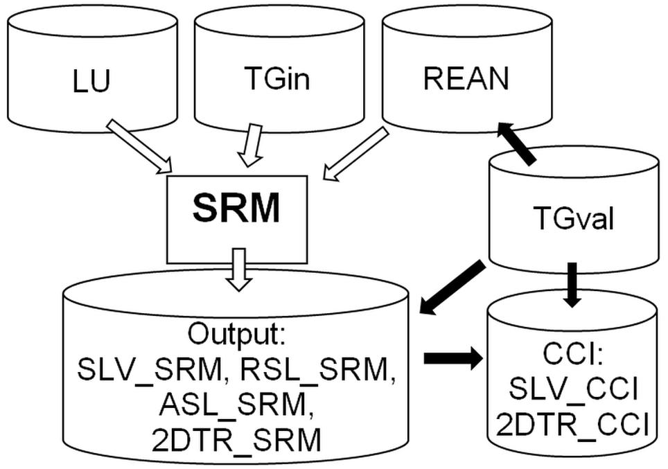
Figure 1. Conceptual chart of model and data flows. SRM, statistical reconstruction model; REAN, reanalysis model data; CCI, CCI satellite altimetry product; LU, land uplift model data; TG, tide gauge data (for input and for validation); SLV, sea level variability; RSL, relative sea level; ASL, absolute sea level; 2DTR, 2D-trends; white arrows, data flow for the SRM; black arrows, validation.

Tide Gauge Data

Sea level measurements at tide gauges provided the empirical basis for the study. Many long records of tide gauge observations exist from the Baltic Sea, some (Stockholm, Saint Petersburg and Świnoujście) stretching back to the 1770s–1810s (Girjatowicz et al., 2016). However, older parts of the series are hardly usable due to gaps and uneven spatial coverage.

For this study, 56 tide gauges with unique records of at least 49 years of data after the year 1900 were identified from the PSMSL dataset (Holgate et al., 2013; Permanent Service for Mean Sea Level [PSMSL], 2016), and supplemented with 4 stations from the Estonian coast, made available from the Estonian Environmental Agency (Figure 2).

FIGURE 2

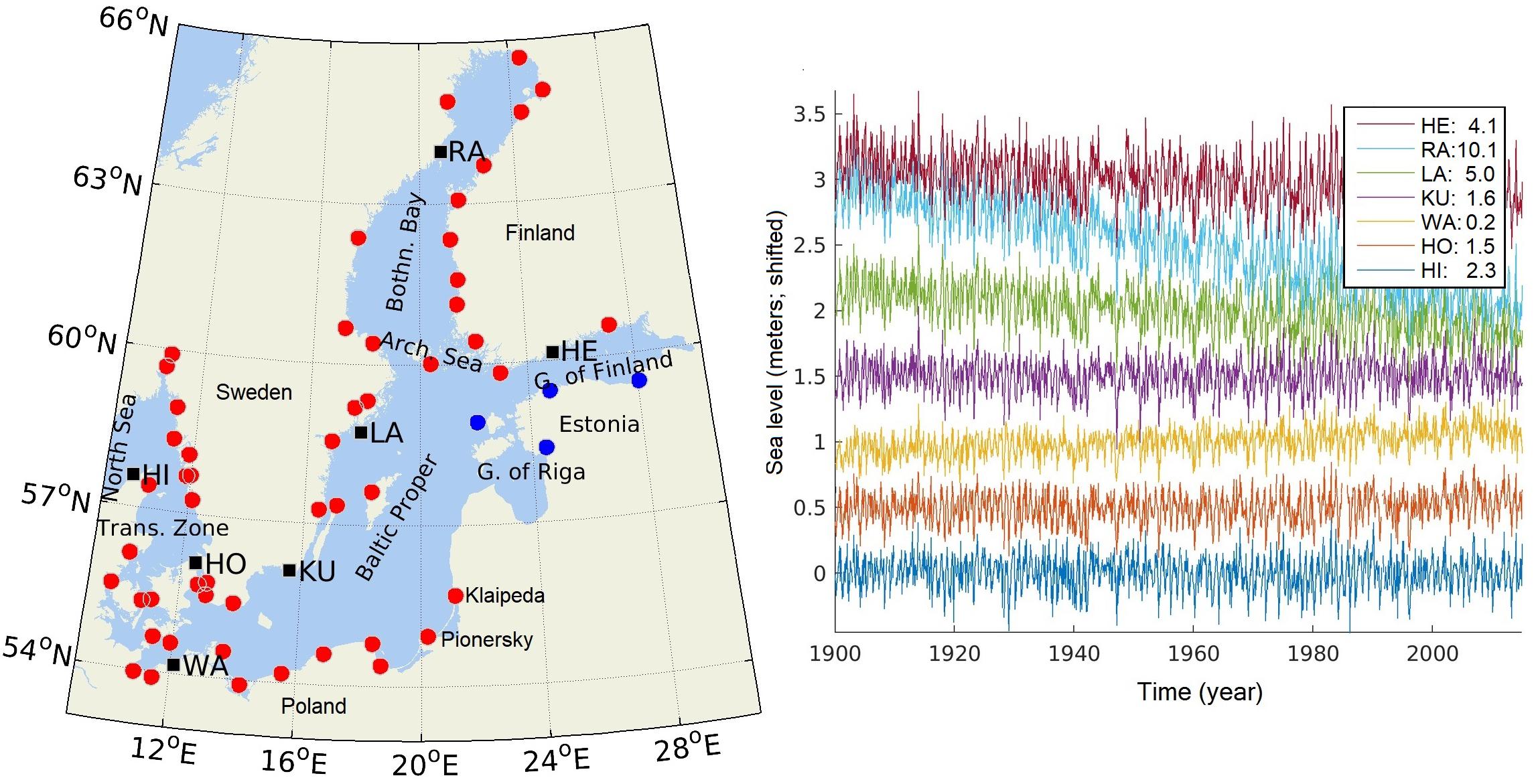
Figure 2. Left: Study area and sea level stations used in the present study (red and black: PSMSL stations, blue: Estonian stations). The seven tide gauge records used for the sea level reconstruction (TGin, black squares) are: Helsinki (HE), Ratan (RA), Landsort (LA), Kungsholmsfort (KU), Warnemünde (WA), Hornbæk (HO), and Hirtshals (HI). All other stations were used for validation (TGval, red and blue circles). Right: Time series of monthly sea level (meters, zero-point shifted for each station) for TGin (1900–2014), showing the influence of land uplift. The value after the station code represents geocentric uplift rate at the location (Vestøl et al., 2019).

Although the oldest Estonian sea level measurements span back to 1842, they have not been yet included in the PSMSL. The main reason has been a poor link to reference systems with known geoid- or geocentric connections (Suursaar and Kall, 2018). The offsets between different height systems (as defined by the mean sea level) around the Baltic Sea may be up to 20 cm (Liibusk et al., 2014). Historically, the Estonian tide gauges have been connected to the Baltic Height System 1977 (BHS77), common in the former Soviet Union (Liibusk et al., 2014). Since 2018, Estonia has changed its height system to the European Vertical Reference System (EVRS), which is based on the level of the Normaal Amsterdams Peil (NAP), and thus, becoming more suitable for PSMSL (Suursaar and Kall, 2018).

The overall data coverage was good (Figure 2). However, the stations are not quite evenly distributed. On the south-eastern coastlines there is a lack of data, most notably before the 1950s. For some of the longest tide gauge records it was possible to partly fill gaps, using neighboring tide gauge records with a high correlation, to allow almost gap-free reconstruction and validation. We used data from Hanstholm to supplement Hirtshals series, Backevik data to supplement Smogen, Varberg to supplement Ringhals, Lemstrom to supplement Foglo/Degerby, Bjorn to supplement Forsmark, Lyokki to supplement Mantyluoto and Koserow to supplement Swinoujscie. Further, data from Landsort Norra was used to extend the Landsort series. The Danish stations Hirtshals, Hornbæk, Aarhus, Fredericia, Slipshavn, Korsør and Gedser only had data until 2012 in the PSMSL archive when this study was performed. Data from the Danish Meteorological Institutes data archives were used to extend the time series to 2014; however, a possible small decrease in the data quality for those last years can occur.

Seven of the longest PSMSL records were used in 2D reconstruction (TGin, Figure 1), and the other records served for validation only (TGval). The seven selected tide gauges were: Hirtshals, Hornbæk, Warnemünde, Kungsholmsfort, Landsort, Ratan and Helsinki (Figure 2). They were selected based on record length, geographical distribution and by using the Akaike information criterion (AIC) method (Burnham and Anderson, 2002).

All linear trends in this paper were obtained as a least square fit of a line to the time series, where the trend is the slope of the line, and the trend uncertainty was set to be the fitting uncertainty.

Reanalysis Data

Available reanalysis products of the Baltic Sea include hydrodynamically modeled sea levels for 20–24 years. Reanalysis data from two hydrodynamic models, the High Resolution Oceanographic Model of the Baltic Sea (HIROMB; Axell and Liu, 2016) and the HIROMB-BOOS Model (HBM; Fu et al., 2012), were considered and compared for this study. These models have both been used for operational forecasting and are therefore calibrated both for normal conditions and extreme events. The HIROMB ocean-ice reanalysis is available in Copernicus Marine Environment Monitoring Service (CMEMS) with 5.5 km horizontal resolution for the period of 1989–2014, while the HBM-based reanalysis covers the years between 1990 and 2009 and is available from the Danish Meteorological Institute. It has a resolution of 6 nautical miles (approx. 11 km), but in the model calculations, a two way nesting in the North Sea – Baltic Sea transition zone with 6 times higher resolution is used. None of the simulations include effects of land uplift and long-term external sea level variability; neither do they assimilate any sea level data. Validation performed within this study showed that both model systems sufficiently reproduced the observed long term variability of the sea level with average RMS error around 6–7 cm and average correlation of 86–88% against tide gauges, and slightly better performance of HBM than HIROMB. For the further parts of this study, data from the HBM model reanalysis were therefore used, here denoted REAN.

Satellite Altimetry Product

Several different sea level change products based on satellite altimetry exist. Here, we focused on the ESA Sea Level CCI ECV v2.0 product² (Quartly et al., 2017; Legeais et al., 2018) for 1993–2014, hereafter denoted as CCI. The CCI record contains monthly fields of sea level variability and linear trend values, here denoted SLV_CCI and 2DTR_CCI, respectively. The two can be combined to form ASL, denoted ASL_CCI. It is developed based on open ocean altimetry data, and constitutes high quality monthly sea level variability and trend analysis for the open ocean.

Input data for the CCI record were corrected for tides, whereas the tidal signal is included in the tide gauge data and the reanalysis model. However, the difference was assumed to be negligible, since this study dealt with monthly mean sea level, and tides are small in the Baltic Sea (generally less than 10 cm, e.g., Samuelsson and Stigebrandt, 1996).

More importantly, the CCI by default includes a Dynamic Atmospheric Correction (DAC), which corrects the altimetry observations for the inverse barometer effect. This sea level signal is observed by the tide gauges, and also included in the ocean model. Therefore 6-hourly DAC fields were downloaded from the CCI-site, averaged to monthly values, and added back into the CCI data. While the trend of the DAC correction was almost zero, the variability on monthly time scales is significant and important for the comparison of sea level variability with tide gauge observations.

Reference Frames and Land Uplift

To assess the separate effects of sea level change and land uplift, accurate information on land deformations, especially from GIA (Steffen and Wu, 2011), is essential in the Baltic Sea region, as the deformations vary throughout the region. In this paper, we mapped both RSL, which is sea level relative to land, and ASL, which is measured in a fixed reference frame referring to the mass center of the Earth. The three data sources – tide gauge observations, satellite observations and reanalysis data based on a hydrodynamic model – all have different reference frames.

Tide gauges measure sea level changes relative to the land on which the tide gauges rest. By itself, a tide gauge cannot tell the difference between local vertical land motion and sea level changes. If a Global Navigation Satellite System (GNSS) station (which uses the satellite navigation signal to measure the position referring to the center of the Earth) is located in connection with the tide gauge, the ASL can be calculated directly (e.g., Nerem et al., 2018). If this kind of data is missing, the vertical land motion (especially GIA effects) can be removed using a land uplift model of the region (Vestøl et al., 2019). It must be taken into account that the corrections from both methods introduce some uncertainties. Since the collocated GNSS station approach is only possible for a limited number of stations in our study area, and includes some uncertainty due to the limited observational GNSS records, than the more general approach of using a land uplift model was used in this study.

The land uplift model used in this study is the NKG2016LU model by the Nordic Geodetic Commission (NKG), which is based on an empirical approach combining GNSS and leveling data in the Nordic region relative to the NKG2016GIA_prel0306 geophysical GIA model (Vestøl et al., 2019). The model was released in two versions: first, uplift relative to geocenter in ITRF2008 reference system (i.e., model version NKG2016LU_abs), and then, by applying a geoid change correction, uplift relative to geoid (NKG2016LU_lev). In this study, the geocentric version was used, and denoted LU (Figure 1). Their difference is not large (∼10%) and not considered important, since it is subtracted from the sea level data consistently over the whole study area. The coastal uncertainty of the NKG2016LU is 0.2 mm/yr (Vestøl et al., 2019), and this uncertainty was propagated into the uncertainty estimates of the ASL change in this study.

For the statistical modeling described below, the sea level variation of the tide gauge data was needed, but also, it had to be ensured that linear trends could be reconstructed. Therefore, RSL from TGin were first corrected for land uplift, giving the ASL. Then, the absolute, linear trend was calculated at each station, and the overall mean trend (MTR) was calculated as the average of the seven linear trend values over the full data period. MTR was assumed to represent the external sea level change signal. MTR was subtracted from the ASL records at the individual stations, resulting in tide gauge sea level variability records with only very small residual trends remaining, SLV_TGin.

Satellite altimetry observations are based on radar measurement of the distance from the satellite to the sea surface, in combination with precise location information of the satellite, in a reference frame referring to the mass center of the Earth. Thus, the satellite altimeter observation represents the ASL.

The reference frame for the reanalysis model is the model bathymetry, which typically refers to mean sea level (of various epochs). Furthermore, the reanalysis data used for this study has a free surface, which reflects surplus river runoff exiting to the Baltic Sea, steric effects generated inside the model area, and the wind setup of the general westerly wind patterns of the study area (Madsen, 2011). This results in a mean sea level setup in the model approximately reflecting the mean sea level setup relative to a geoid. The sea level difference due to a tilt from the Danish Straits toward NE part of the Baltic Sea can reach about 40 cm (Figure 3). The REAN data do not include external sea level change. In this study, only the detrended monthly variability fields of the REAN data were used, and therefore, the somewhat arbitrary reference level was assumed not to be important.

FIGURE 3

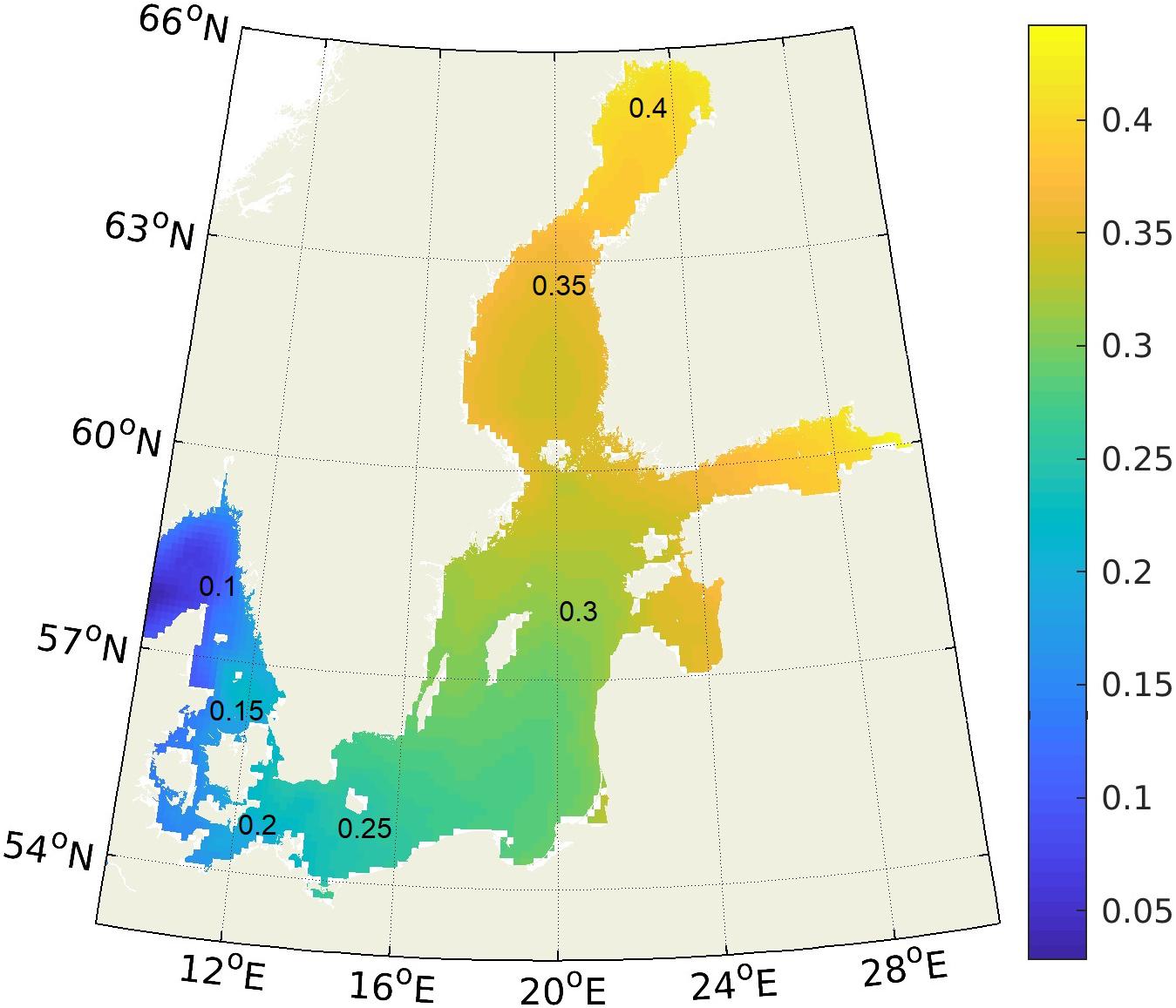
Figure 3. Mean sea level (meters) in the Baltic Sea 1990–2009 from the HBM ocean model reanalysis.

Statistical Model

For the statistical reconstruction of the sea level fields, a multiple linear regression was used, based on Madsen et al. (2007, 2015). With this method, the statistical model uses a training data set to calculate the optimal weights that each of the selected tide gauges should have in order to reconstruct the sea level with the lowest mean square differences. The optimal weights are calculated for each 2D grid point and the statistical model is thus able to reconstruct the 2D sea level field using only the tide gauge observations.

In the present study, SLV_TGin (7 single points, long time series), as well as a constant trend, were trained against the model reanalysis data (REAN, 2-dimensional, limited time period) (Figure 1). When calculating the statistical model coefficients, each point in the REAN 2D grid was treated individually, and the seven SLV_TGin records and the constant trend were linearly combined to fit the time series of REAN data in the point, in an optimal, damped least squares sense. A damping coefficient of 0.5 was selected to stabilize the model weights.

The result was a set of seven 2D fields of weights for the SLV_TGin records, and a 2D field of values for the overall mean trend, forming the statistical model, SRM. The RMS fitting error of the statistical model was 5 cm for tide gauges in most of the Baltic Sea, increasing to 7 cm for stations in the far northern and eastern parts. The weights of the overall mean trend were negative and small, with absolute values less than 0.06 mm/yr in all locations.

After derivation of the spatial regression patterns of this statistical model, the full monthly 2D sea level variability fields (SLV_SRM) were reconstructed. Then ASL change (ASL_SRM) was calculated by adding the overall mean sea level trend, MTR, back in, and finally, the effect of land uplift (LU) was taken into account to get the RSL change (RSL_SRM).

Results

Reconstructed Sea Level

As described above, the monthly mean sea level in the approximately 11 × 11 km grid (same as for the REAN) was reconstructed for the entire Baltic Sea from 1900 to 2014, using SRM. Gaps were allowed, where observations from the seven tide gauges were missing (in total 41 months or 3%) with the biggest gaps in the 1980s and 1990s. The reconstruction allowed assessment of the monthly and annual sea level for all parts of the Baltic Sea, including those with limited tide gauge coverage, relative to the coast or absolute. It also allowed consistent assessment of the area-averaged sea level (Figure 4). The ASL rose over the last century (to be quantified further below), but with inter-annual variability of approximately the same magnitude. It is thus clear that a proper assessment of trends is sensitive to the period for which the trend is calculated.

FIGURE 4

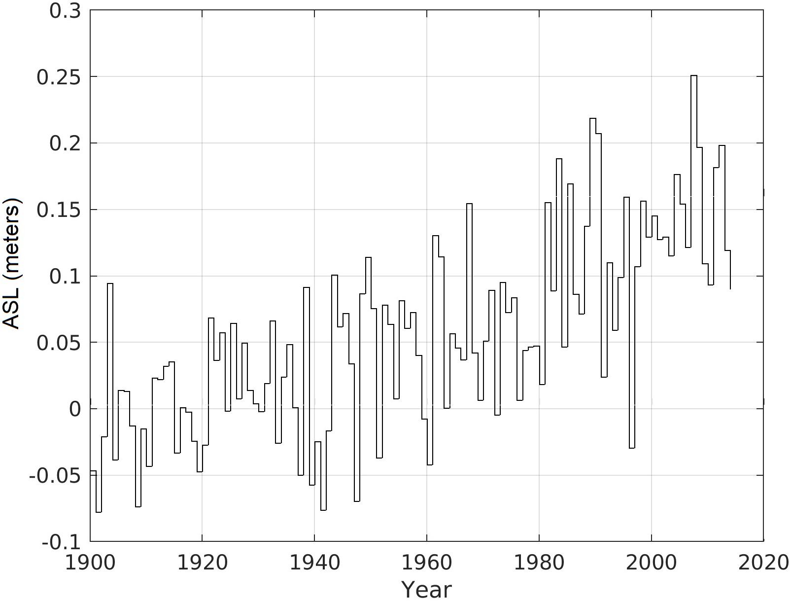
Figure 4. Temporal variations in area averaged annual ASL_SRM in the Baltic Sea.

The reconstructed datasets of 2D relative and absolute monthly mean sea level generated for this study, as well as the calculated linear trends (RSL_SRM, ASL_SRM and 2DTR_SRM), are available from Madsen et al. (2019).

Validation of Reconstruction Against Tide Gauges

SLV_SRM was validated using the 56 independent tide gauge records (TGval). For each record, the linear trend of the station was removed, forming SLV_TGval, and the closest water grid point of the SRM was found. The two time-series were used for the common time span. The average correlation was 96%, and the average RMS difference was 3.8 cm (Figure 5). Furthermore, few TGval stations with poor statistics stood out. Especially, Klaipeda had an RMS error of 7 cm, compared to 4 cm at the nearest station, Pionersky, and also showed a much lower correlation coefficient. We speculate that this was due to the influence of the nearby Curonian Lagoon on the Klaipeda tide gauge observations. The RMS difference was also higher in the northern Bothnian Bay (5–6 cm), probably related to the influence of seasonal sea ice. The correlation was 86–95% in the very dynamic North Sea – Baltic Sea (NS-BS) transition zone. Even with these limitations, the statistical reconstruction (SRM) showed better validation results when compared to independent tide gauge observations (TGval) than the original reanalysis product (REAN, which has average correlation 88%, and RMS difference 6 cm for the same stations, but for 1990–2009).

FIGURE 5

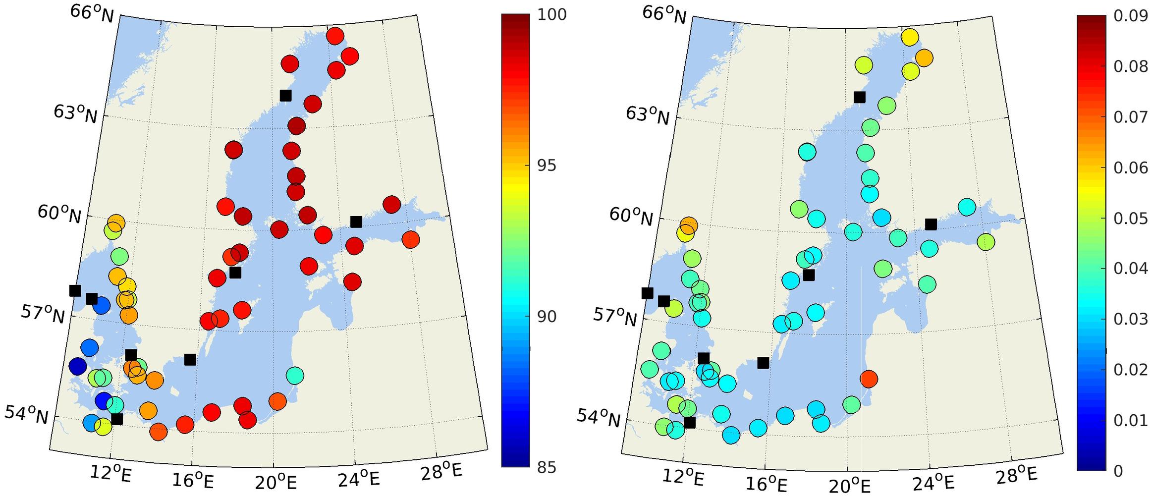
Figure 5. Correlation (%, left) and RMS differences (meters, right) between SLV_TGval and the nearest neighboring point of SLV_SRM. Colored circles: validation stations. Black squares: TGin stations.

Validation of Satellite Altimetry Variability and Area of High Quality Data

With the high correspondence between SLV_SRM and SLV_TGval, we determined that the statistical reconstruction was suitable for validation of the temporal and spatial variability of satellite products.

When comparing SLV_SRM with the CCI product (SLV_CCI), the correlation in the central Baltic Sea was generally high, with lower values in the NS-BS transition zone (Figure 6, right panel). There, the CCI was most likely affected by lack of data and interpolation over large scales. The RMS differences showed increased values of 7–12 cm in the northern Bothnian Bay, eastern Gulf of Finland, and south-eastern Gulf of Riga, (partly due to sea ice effects), as well as in parts of the NS-BS transition zone (Figure 6, left panel). Both correlation and RMS differences between SLV_TGval and SLV_CCI (nearest neighboring point) in all cases closely followed that of neighboring grid points of the statistical reconstruction, indicating that the main source of uncertainty is the CCI. The uncertainty is only slightly higher in the Archipelago Sea, indicating that the CCI was able to capture monthly sea level variations in this demanding area.

FIGURE 6

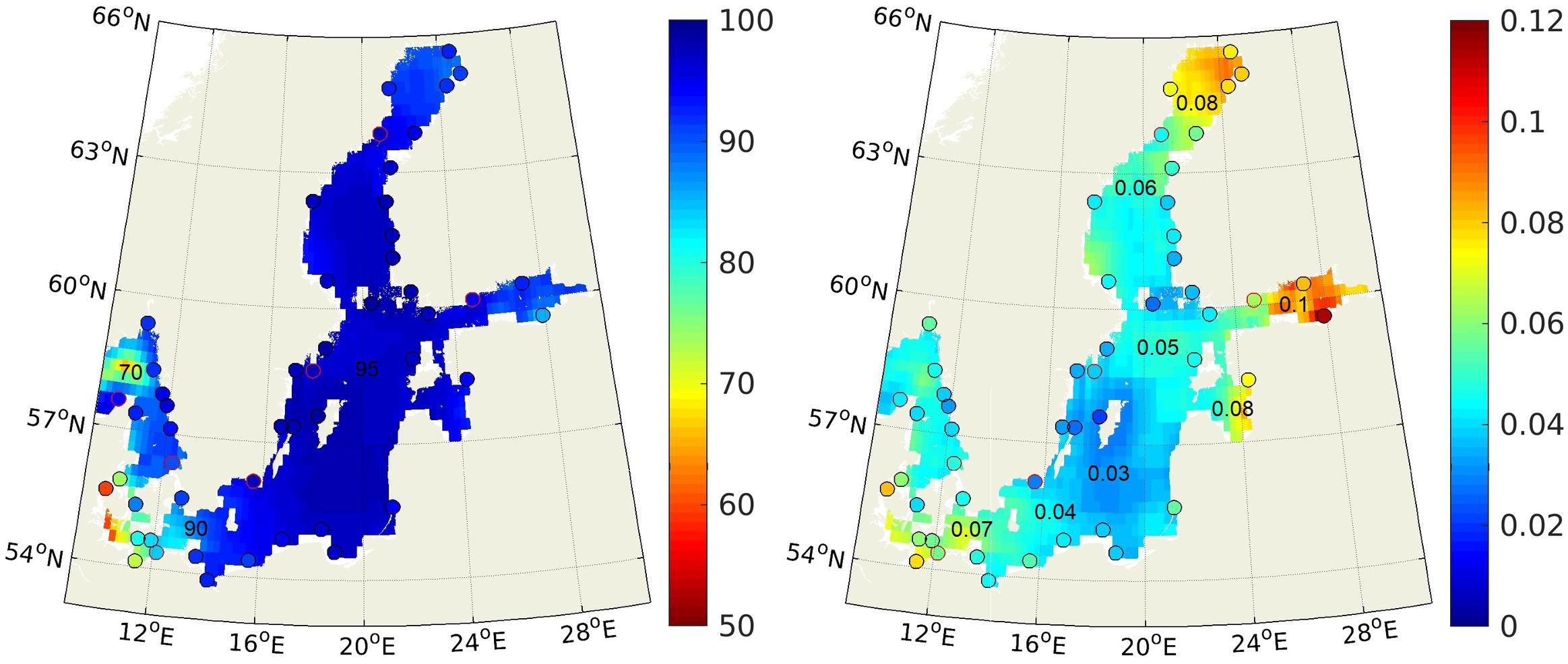
Figure 6. Validation of monthly SLV_CCI against SLV_TGval (dots with black edges, nearest neighboring point), SLV_TGin (dots with red edges, nearest neighboring point) and reconstructed sea level (colored areas). Left: correlation (%), Right: RMS difference (meters).

In order to find the areas with statistically reliable (hereafter “adequate”) data quality, the CCI data was masked if the RMS difference between SLV_CCI and SLV_SRM was larger than 6 cm or the correlation was below 90%. These thresholds were selected to approximately match the quality level of the statistical reconstruction and the reanalysis product. The area with adequate data quality encompassed the Baltic Proper, the southern Gulf of Bothnia, the western Gulf of Finland and western Gulf of Riga (Figure 7, left).

FIGURE 7

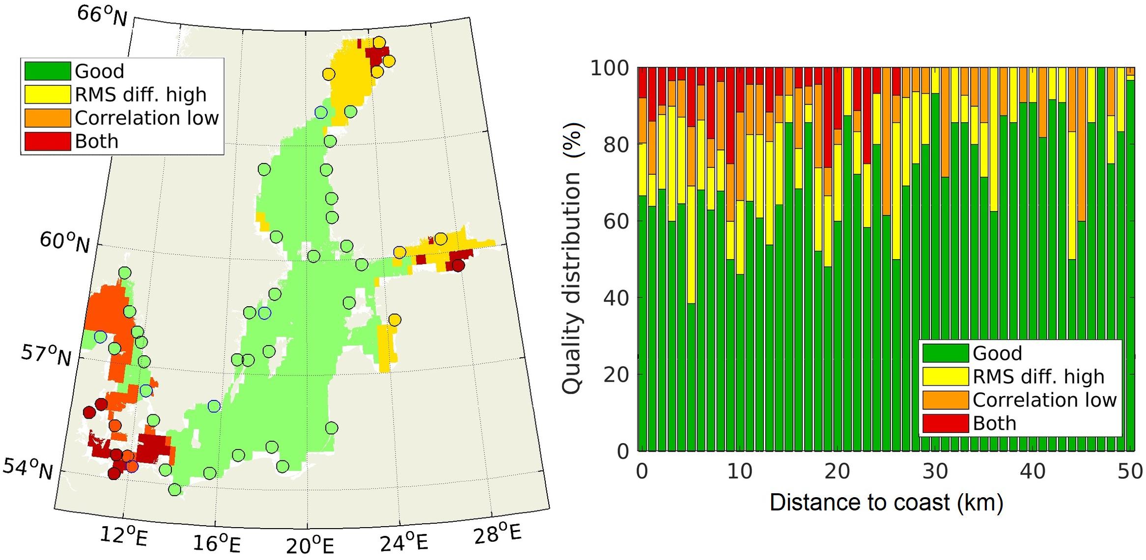
Figure 7. Left: CCI data evaluation showing the areas with adequate data quality according to this study, and the areas with low correlation and/or high RMS difference to SLV_SRM (colored areas) and SLV_TG (circles). Right: percentage of areas with different quality classes versus distance to the coast.

Some relation was seen between the distance to the nearest coast and the amount of adequate data. In the zone 0–15 km from the shore, about 35% of the points in the Baltic Sea region were considered to be of degraded quality. The share decreased to about 10% in the 30–50 km offshore zone (Figure 7, right).

Sea Level Trends Derived From Satellite Altimetry

In order to make trustworthy assessments of the sea level trend, one must be able to reproduce the sea level variability. We considered that the areas where the SLV_CCI showed adequate quality were also suitable for trend estimation, considering that the CCI was designed for this task. The CCI linear sea level trend over the period 1993–2015 is shown in Figure 8, with dotted areas indicating areas of decreased quality of SLV_CCI. The CCI-based linear sea level trend was calculated as the overall average value over the area with adequate quality of SLV_CCI. It was 4.0 mm/yr for this period, with a standard deviation of 0.5 mm/yr. The error information provided with the CCI shows an error level of 1.0–1.3 mm/yr in this area (mean 1.2 mm/yr). The combined error (taking into account two sources) is therefore approximately $\sqrt{{0.5}^2+{1.2}^2}$ = 1.3 mm/yr over the study period and for the area with trustworthy data.

FIGURE 8

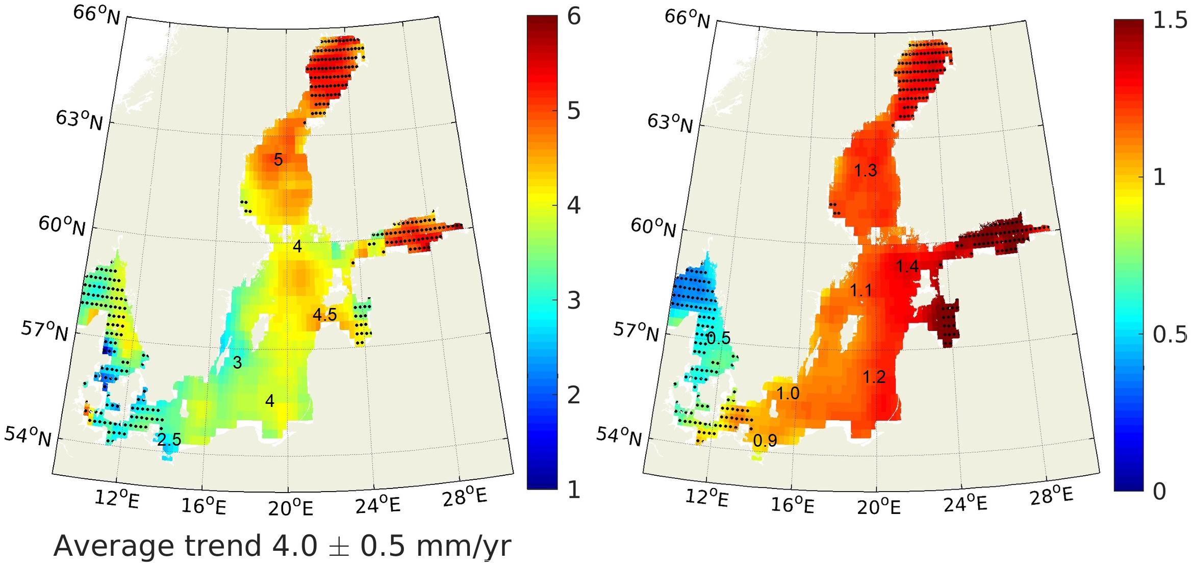
Figure 8. Left: Spatial distribution of linear sea level trends in the Baltic Sea according to the CCI (1993–2015, mm/yr). Right: Corresponding trend error (mm/yr) fields as provided by the CCI. Black dotted areas denote the regions with decreased data quality of SLV_CCI according to this study.

The sea level trend error field from the CCI data did not reflect the assessment of areas with adequate data quality according to this study. Uncertainty sources from interpolation errors in the coastal areas and in the ice affected regions were not taken into account. Also, the provided uncertainty field had very low values in the North Sea – Baltic Sea transition zone (Figure 8, right).

Trends of the 20th Century Reconstruction

The hundred year’s RSL_SRM trend from 1915 to 2014 was, as expected, dominated by the land uplift signal (Figure 9). Hence, decreasing sea level trends occurred in large parts of the Baltic Sea, reaching up to −9 mm/yr in the northern Bothnian Bay.

FIGURE 9

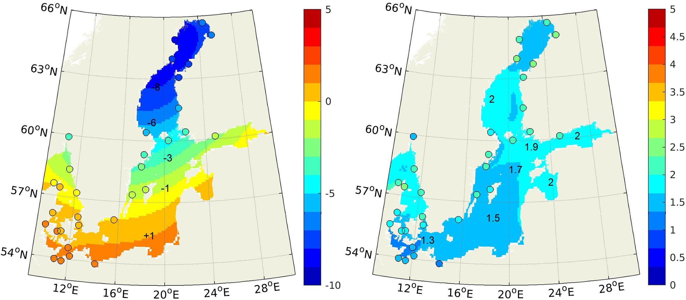
Figure 9. Linear sea level trends (mm/yr) derived from SRM and from tide gauges, 1915–2014. Left: relative to land; right: absolute values. Note that only tide gauges with adequate record length have been included. Also note that the trends in tide gauges may exceed (up to 1 mm/yr) the trends in the offshore area.

There was a close correspondence between the trends observed at the tide gauges and those at the neighboring grid cells of relative 2DTR_SRM. For the eastern Baltic Sea, which lacks very long observational records, the trend increased toward south-south-east, with coastal values increasing from −2 mm/yr on the north-western Estonian coast to +1 mm/yr at the Polish coast.

The ASL change of the same hundred years’ time frame was much more uniform across the Baltic Sea. The observations (TGval) showed absolute linear trends of 1.2–2.5 mm/yr. Fitting uncertainties of the linear trends at the individual stations went up to 0.2 mm/yr with the highest values being located at individual stations in the northern Bothnian Bay as well as in the outer zone bordering with the North Sea. Similarly, the statistical model showed linear trends (absolute 2DTR_SRM for 1915–2014) of 1.2–2.1 mm/yr, but in a slightly different pattern. The highest values occurred in the stretch from Kattegat over the central Baltic Proper, and into the gulfs of Finland and Riga. These differences were within the uncertainty range. They could have occurred due to uncertainties in the statistical reconstruction, small-scale variations in land uplift field, or due to changes in wind setup. When comparing these absolute trends with absolute trends derived using other methods, the uncertainty of the uplift model must be taken into account, yielding a total uncertainty of approximately $\sqrt{{0.2}^2+{0.2}^2}$ = 0.3 mm/yr.

Comparison in Satellite Era

For the satellite era, the overall averaged ASL change rates from the regression model (absolute 2DTR_SRM for 1993–2014) and satellite data (2DTR_CCI) are compared in Table 1. The fitting uncertainty is largely increased for this shorter time period. This uncertainty mainly occurs due to large interannual variability (see also section 3.1). Focusing on the satellite era, the ASL trend was higher in the latest decades than in the 100-year average values (1.2–2.5 mm/yr for 1915–2014). The reconstruction-derived trend was 3.4 ± 0.7 mm/yr for 1993–2014, and the highest trend estimate (4.0 ± 1.3 mm/yr over 1993–2015) was offered by CCI.

TABLE 1

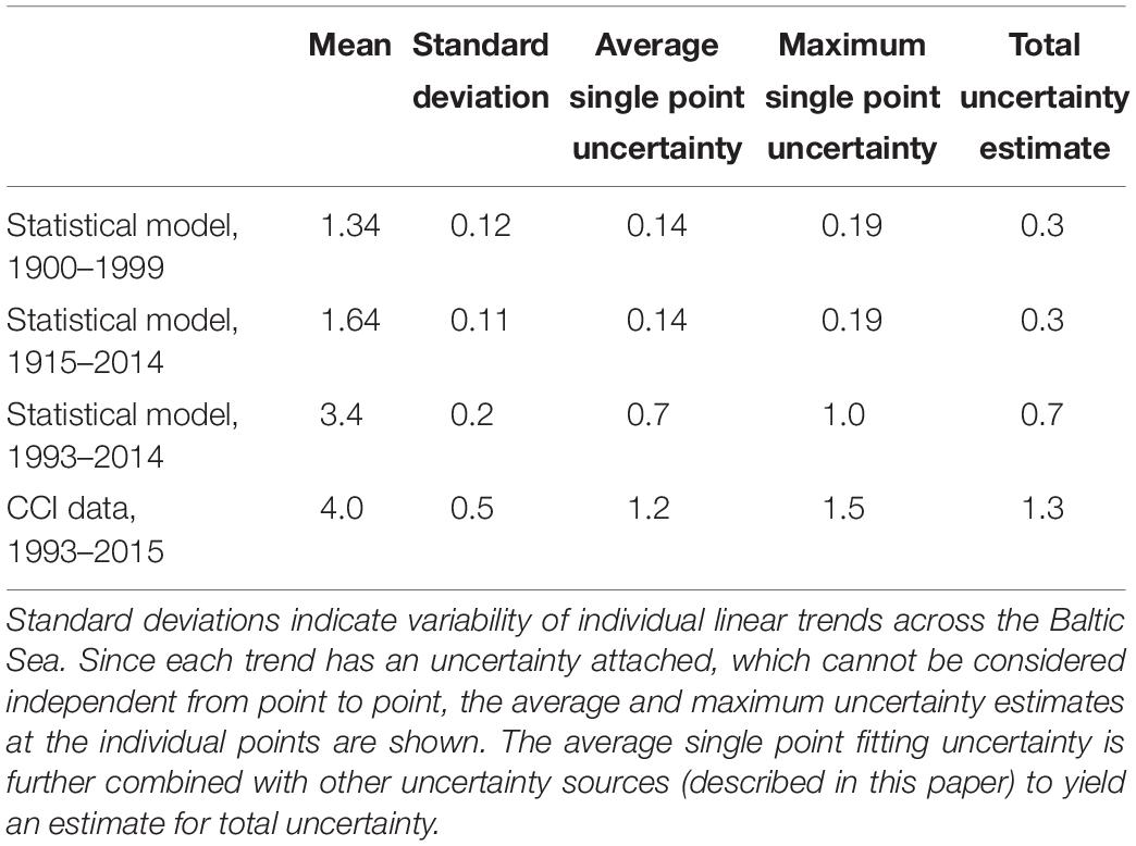
Table 1. Mean linear ASL change rates in the Baltic Sea from SRM and CCI (mm/yr).

Discussion

Reconstruction Versus Reanalysis

The reconstructed sea level (SRM) validated well against the tide gauge data (TGval) and provided good spatial data coverage. However, compared to the hydrodynamic model reanalysis (REAN), it had two main weaknesses. The SRM was sensitive to the data quality, coverage, and completeness, and it only provided information on the sea level, whereas a reanalysis can provide 3D fields of temperature, salinity and ocean currents to complement the sea level fields. The benefits of the statistical method are in its’ good performance for the region and low computational costs. Also, this study demonstrated that a lot of information is available in the tide gauge records, which can be assimilated into model-based reanalyses in the future.

The SRM performed well in the open waters of the Baltic Sea, but it was challenged by the complex hydrodynamics in the North Sea – Baltic Sea transition zone. It mainly occurred due to shorter correlation scales in time and space, and less good representation in the input reanalysis model. This zone puts high demands on any ocean model, and also on the satellite altimetry products. However, the zone is densely covered by tide gauges and allows detailed validation. Future developments will require very high resolution modeling with high quality bathymetry and atmospheric forcing using e.g., UERRA (Ridal et al., 2017) reanalysis. Downscaling of ERA5 (within the Copernicus Climate Change initiative) is likely to provide even more detailed atmospheric forcing.

Land Uplift

Reconstruction of ASL trends relies on land uplift models, especially in the areas with a large land uplift signal, such as the Baltic Sea area. The newly developed land uplift model (Vestøl et al., 2019) helps to improve the determination of ASL change from tide gauges in the Baltic region. However, small errors could still occur e.g., due to un-modeled (local) land subsidence, that can introduce errors in the tide gauge records. An alternative approach would be to use collocated GNSS station data, as it was done by Richter A. et al. (2012). However, the uncertainties of that procedure are still relatively high, mainly due to the limited temporal coverage of the GNSS stations. In future situations, when the GNSS stations have the opportunity to continue their recordings for a longer period of time, the observed land uplift can be used instead of or in combination with a land uplift model. Finally, there may be small systematic errors in the connection of the geodetic height system to the international geodetic reference frame.

Satellite Altimetry in the Coastal Seas

The results presented in this paper demonstrate that the satellite altimetry observations can provide valuable information in the coastal sea for studying the long term linear sea level trends, and the two estimates of sea level trends (satellite versus reconstructed) agreed within the uncertainty limits. So far, the time series of the CCI is still relatively short considering the long-term variability in sea level and the observed global acceleration (Church and White, 2006; Sallenger et al., 2012). It is especially true in semi-enclosed areas like the Baltic Sea, where interannual sea level variability is higher than in the open ocean (Suursaar and Kall, 2018). It is also clear that the Baltic Sea is a challenging area for global satellite products due to lack of open sea spaces, complex coastlines, and presence of small islands. These features are demanding for both the along-track satellite processors and for the gridding and interpolation procedures (see e.g., Passaro et al., 2014; Ablain et al., 2015). A dedicated regional CCI would be beneficial to overcome these limitations and to extend the use of satellite observations at coast.

Yet another challenge for satellite products is the occurrence of seasonal sea ice e.g., in the Bothnian Bay and Gulf of Finland (e.g., Vihma and Haapala, 2009). The gaps due to missing data may last for several months in each year, which leads to a higher uncertainty in the linear sea level trends (Figure 8). In order to properly determine the sea level trends for the entire Baltic Sea, it is necessary to have an estimate of the sea level in ice covered areas, which would require a dedicated satellite product.

Sea Level Trends

The rates of ASL change found for the Baltic Sea (1.34 mm/yr in 1900–1999; 1.64 mm/yr in 1915–2014; Table 1) were similar to the global average of the same time period (1.7 mm/yr in 1900–2010; IPCC, 2013). For the 20th century, the area averaged ASL change for the entire Baltic Sea was 1.3 ± 0.3 mm/yr. For the satellite era (1993–2014), the linear trends derived from the reconstruction (3.4 ± 0.7 mm/yr) matched those of the CCI (4.0 ± 1.4 mm/yr for 1993–2015) within the uncertainty limits. While the century-long trend was quite stable, the trend of the satellite era is highly sensitive to interannual variability (Figure 4).

When discussing spatial variations in absolute trend reconstruction, the trend values were higher (by ∼0.5 mm/yr) in the (“lower quality”) far ends of the elongated Baltic Sea: in the Bothnian Bay, Gulf of Finland and Gulf of Riga (Figure 9). They were higher also in the Kattegat, just before the narrowest parts of the Danish Straits, but less high in the south-western Baltic Sea. This was connected to the peculiarities of water exchange processes of the Baltic Sea in conditions of climatologically prevailing south-westerlies in that region (Suursaar and Kullas, 2006). Within the Baltic Sea, the sea level amplitudes (variability) of both external (i.e., long-term water surplus variations) and internal sea level oscillations (occurring as a half-wave-length oscillator) increase in the far ends of the sea, and decreases in the central, nodal part (Samuelsson and Stigebrandt, 1996). This has also been illustrated in several hydrodynamic modeling studies (e.g., Meier et al., 2004; Suursaar and Kullas, 2006). When comparing between datasets, the RMS difference is likely to increase when trends and sea level variability increase. On the other hand, neglecting those “lower quality” areas (with higher absolute trends) may lower the average Baltic Sea level trend estimates.

When comparing the obtained sea level change rates with the global ones, the focus should be on the ASL change. However, when assessing the impacts of ongoing climate change on the coast and coastal societies, the main focus should be on the RSL change. So far, the influence of global sea level change is largely canceled out by GIA effects in the central Baltic Sea area. However, with future global sea level change and its acceleration (IPCC, 2013), wider areas in the Baltic Sea will experience RSL change impacts as well.

Conclusion

This study on both ASL and RSL change in the entire Baltic Sea provides a basis to cope with anticipated climate-related sea level changes in the future. Using a statistical model, monthly mean sea level was reconstructed for the entire Baltic Sea in an 11 × 11 km grid from 1900 to 2014. The reconstructed monthly sea level variability was successfully validated using 56 tide gauge records and against satellite altimetry (CCI) products. The absolute and relative 2D sea level trend fields were calculated. It appeared that sea level data from satellite altimetry can be successfully used for assessing monthly sea level variability in the Baltic Sea, and that linear sea level trends from the 2D statistical reconstruction and satellite altimetry agreed with each other within the uncertainty range. It also appeared that coastal zones, especially in the areas with seasonal sea ice and the areas of high natural variability, need special treatment. However, the increased uncertainty in such areas was not reflected in the trend error field provided with the CCI. The RSL trend (with values down to −9 mm/yr in the northern Bothnian Bay over 1915–2014) was dominated by postglacial uplift of that area. The area averaged ASL change for the entire Baltic Sea was 1.3 ± 0.3 mm/yr in the 20th century. For the satellite era (1993–2014), the linear trends derived from the reconstruction (3.4 ± 0.7 mm/yr) matched those of the CCI (4.0 ± 1.4 mm/yr for 1993–2015) within the uncertainty limits. Although shortness of the latter made trend estimation highly sensitive to the variability, the sea level change rates found in the study confirmed their acceleration over the last decades. Further refinement of the models and inclusion of new data hopefully enables more reliable results in the future.

Author Contributions

KM was responsible for compiling the data, modeling, and writing the manuscript. JH, JS, and PK contributed to the data analysis, modeling, and writing. ÜS provided additional data and contributed to the writing.

Funding

The research leading to these results has received funding from the Baltic Sea Check Point project under contract number EASME/EMFF/2014/1,3,1,1/LOT 3/SI2.708189, Estonian Research Council grant PUT1439, and the Danish Government grant Klimaatlas.

Conflict of Interest Statement

The authors declare that the research was conducted in the absence of any commercial or financial relationships that could be construed as a potential conflict of interest.

Acknowledgments

In situ observations have been obtained from PSMSL (http://www.psmsl.org/data/obtaining/), the Estonian Environment Agency and the Copernicus Marine Environment Monitoring Service, supplemented with data from the Danish Meteorological Institute. Satellite observations were obtained from the ESA Sea Level CCI, and the uplift data from the NKG (Vestøl et al., 2019). We thank the two reviewers for their suggestions that helped to improve and clarify the manuscript, as well as Beverly Bishop and April Bernhardsgrütter for their language advice.

Footnotes

1. ^ http://www.eea.europa.eu/data-and-maps/indicators/sea-level-rise-2/assessment
2. ^ www.esa-sealevel-cci.org/products/

References

Ablain, M., Cazenave, A., Larnicol, G., Balmaseda, M., Cipollini, P., Faugère, Y., et al. (2015). Improved sea level record over the satellite altimetry era (1993–2010) from the climate change initiative project. Ocean Sci. 11, 67–82. doi: 10.5194/os-11-67-2015

CrossRef Full Text | Google Scholar

Axell, L., and Liu, Y. (2016). Application of 3-D ensemble variational data assimilation to a Baltic Sea reanalysis 1989–2013. Tellus 68A:24220. doi: 10.3402/tellusa.v68.24220

CrossRef Full Text | Google Scholar

Bonaduce, A., Pinardi, N., Oddo, P., Spada, G., and Larnicol, G. (2016). Sea-level variability in the mediterranean Sea from altimetry and tide gauges. Clim. Dyn. 47, 2851–2866. doi: 10.1007/s00382-016-3001-2

CrossRef Full Text | Google Scholar

Burnham, K. P., and Anderson, D. R. (2002). Model Selection and Multimodel Inference: A Practical Information-Theoretic Approach, 2nd Edn. Berlin: Springer-Verlag.

Google Scholar

Calafat, F. M., and Jordà, G. (2011). A Mediterranean sea level reconstruction (1950–2008) with error budget estimates. Glob. Planet. Change 79, 118–133. doi: 10.1016/j.gloplacha.2011.09.003

CrossRef Full Text | Google Scholar

Church, J. A., and White, N. J. (2006). A 20th century acceleration in global sea-level rise. Geophys. Res. Lett. 33, 1–4. doi: 10.1029/2005GL024826

PubMed Abstract | CrossRef Full Text | Google Scholar

Ekman, M. (1996). A consistent map of the postglacial uplift of fennoscandia. Terra Nova 8, 158–165. doi: 10.1111/j.1365-3121.1996.tb00739.x

CrossRef Full Text | Google Scholar

Fu, W., She, J., and Dobrynin, M. (2012). A 20-yr reanalysis Experiment in the Baltic Sea using three dimensional variational (3DVAR) method. Ocean Sci. 8, 827–844. doi: 10.5194/os-8-827-2012

CrossRef Full Text | Google Scholar

Girjatowicz, J. P., Świa̧tek, M., and Wolski, T. (2016). The influence of atmospheric circulation on the water level on the southern coast of the Baltic Sea. Int. J. Climatol. 36, 4534–4547. doi: 10.1002/joc.4650

CrossRef Full Text | Google Scholar

Holgate, S. J., Matthews, A., Woodworth, P. L., Rickards, L. J., Tamisiea, M. E., Bradshaw, E., et al. (2013). New data systems and products at the permanent service for mean sea level. J. Coast. Res. 29, 493–504. doi: 10.2112/JCOASTRES-D-12-00175.1

CrossRef Full Text | Google Scholar

Hünicke, B., Zorita, E., Soomere, T., Madsen, K. S., Johansson, M., and Suursaar, Ü (2015). “Recent change – sea level and wind waves,” in Second Assessment of Climate Change for the Baltic Sea Basin, ed. BACC II Author Team, (Berlin: Springer), 155–186. doi: 10.1007/978-3-319-16006-1-9

CrossRef Full Text | Google Scholar

IPCC (2013). “Fifth assessment report (AR5),” in Climate Change 2013: The Physical Science Basis. Contribution of Working Group I to the Fifth Assessment Report of the Intergovernmental Panel on Climate Change, eds T. F. Stocker, D. Qin, G. K. Plattner, M. Tignor, S. K. Allen, J. Boschung, et al. (Cambridge: Cambridge University Press).

Google Scholar

Johansson, M., Kahma, K. K., Boman, H., and Launiainen, J. (2004). Scenarios for sea level on the finnish coast. Boreal. Environ. Res. 9, 153–166.

Google Scholar

Legeais, J.-F., Ablain, M., Zawadzki, L., Zuo, H., Johannessen, J. A., Scharffenberg, M. G., et al. (2018). An improved and homogeneous altimeter sea level record from the ESA climate change Initiative. Earth Syst. Sci. Data 10, 281–301. doi: 10.5194/essd-10-281-2018

CrossRef Full Text | Google Scholar

Liibusk, A., Kall, T., Ellmann, A., and Kõuts, T. (2014). “Correcting tide gauge series due to land uplift and differences between national height systems of the baltic sea countries,” in Proceedings of the 2014 IEEE/OES Baltic International Symposium (BALTIC), (Piscataway, NJ: IEEE), doi: 10.1109/BALTIC.2014.6887828

CrossRef Full Text | Google Scholar

Madsen, K. S. (2011). Recent and Future Climatic Changes of the North Sea and the Baltic Sea – Temperature, Salinity, and Sea Level. Latvia: LAMBERT Academic Publishing.

Google Scholar

Madsen, K. S., Høyer, J. L., Fu, W., and Donlon, C. (2015). Blending of satellite and tide gauge sea level observations and its assimilation in a storm surge model of the North Sea and Baltic Sea. J. Geophys. Res. 120, 6405–6418. doi: 10.1002/2015JC011070

PubMed Abstract | CrossRef Full Text | Google Scholar

Madsen, K. S., Høyer, J. L., Suursaar, Ü, She, J., and Knudsen, P. (2019). Reconstructed 2D relative and absolute monthly mean sea level of the Baltic Sea 1900-2014, and related linear trends. Dataset

Google Scholar

Madsen, K. S., Høyer, J. L., and Tscherning, C. C. (2007). Near-coastal satellite altimetry: sea surface height variability in the North Sea–Baltic Sea area. Geophys. Res. Lett. 34:L14601. doi: 10.1029/2007GL029965

CrossRef Full Text | Google Scholar

Meier, H. E. M., Broman, B., and Kjellström, E. (2004). Simulated sea level in past and future climates of the Baltic Sea. Clim. Res. 27, 59–75. doi: 10.3354/cr027059

CrossRef Full Text | Google Scholar

Milne, G. A., Gehrels, W. R., Hughes, C. W., and Tamisiea, M. E. (2009). Identifying the causes of sea-level change. Nat. Geosci. 2, 471–478. doi: 10.1038/ngeo544

CrossRef Full Text | Google Scholar

Nerem, R. S., Beckley, B. D., Fasullo, J. T., Hamlington, B. D., Masters, D., and Mitchum, G. T. (2018). Climate-change-driven accelerated sea-level rise detected in the altimeter era. PNAS 115, 2022–2025. doi: 10.1073/pnas.1717312115

PubMed Abstract | CrossRef Full Text | Google Scholar

Olivieri, M., and Spada, G. (2016). Spatial sea-level reconstruction in the Baltic Sea and in the pacific Ocean from tide gauges observations. Ann. Geophys. 59:0323.

Google Scholar

Passaro, M., Cipollini, P., Vignudelli, S., Quartly, G. D., and Snaith, H. M. (2014). ALES: a multi-mission adaptive subwaveform retracker for coastal and open ocean altimetry. Remote Sens. Environ. 145, 173–189. doi: 10.1016/j.rse.2014.02.008

CrossRef Full Text | Google Scholar

Permanent Service for Mean Sea Level [PSMSL], (2016). Tide Gauge Data. Available at: http://www.psmsl.org/data/obtaining/ (accessed January 7, 2016).

Google Scholar

Quartly, G. D., Legeais, J.-F., Ablain, M., Zawadzki, L., Fernandes, M. J., Rudenko, S., et al. (2017). A new phase in the production of quality-controlled sea level data. Earth Syst. Sci. Data 9, 557–572. doi: 10.5194/essd-9-557-2017

CrossRef Full Text | Google Scholar

Richter, A., Groh, A., and Dietrich, R. (2012). Geodetic observation of sea-level change and crustal deformation in the Baltic Sea region. Phys. Chem. Earth 53-54, 43–53. doi: 10.1016/j.pce.2011.04.011

CrossRef Full Text | Google Scholar

Richter, K., Nilsen, J. E. Ø, and Drange, H. (2012). Contributions to sea level variability along the norwegian coast for 1960–2010. J. Geophys. Res. 117:C05038. doi: 10.1029/2011JC007826

CrossRef Full Text | Google Scholar

Ridal, M., Olsson, E., Unden, P., Zimmermann, K., and Ohlsson, A. (2017). HARMONIE Reanalysis Report of Results and Dataset. UERRA Deliverable D2.7. Available at: http://www.uerra.eu/publications/deliverable-reports.html

Google Scholar

Sallenger, A. H. Jr., Doran, K. S., and Howd, P. A. (2012). Hotspot of accelerated sea-level rise on the Atlantic coast of North America. Nat. Clim. Change 2:884. doi: 10.1038/nclimate1597

CrossRef Full Text | Google Scholar

Samuelsson, M., and Stigebrandt, A. (1996). Main characteristics of the long-term sea level variability in the Baltic Sea. Tellus 48A, 672–683. doi: 10.3402/tellusa.v48i5.12165

CrossRef Full Text | Google Scholar

Santamaría-Gómez, A., Gravelle, M., Dangendorf, S., Marcos, M., Spada, G., and Wöppelmann, G. (2017). Uncertainty of the 20th century sea-level rise due to vertical land motion errors. Earth Planet. Sci. Lett. 473, 24–32. doi: 10.1016/j.epsl.2017.05.038

CrossRef Full Text | Google Scholar

Simon, K. M., Riva, R. E. M., Kleinherenbrink, M., and Frederikse, T. (2018). The glacial isostatic adjustment signal at present day in northern Europe and the British isles estimated from geodetic observations and geophysical models. Solid Earth 9, 777–795. doi: 10.5194/se-9-777-2018

CrossRef Full Text | Google Scholar

Spada, G. (2017). Glacial isostatic adjustment and contemporary sea level rise: an overview. Surv. Geophys. 38, 153–185. doi: 10.1007/s10712-016-9379-x

CrossRef Full Text | Google Scholar

Steffen, H., and Wu, P. (2011). Glacial isostatic adjustment in fennoscandia – a review of data and modeling. J. Geodyn. 52, 169–204. doi: 10.1016/j.jog.2011.03.002

CrossRef Full Text | Google Scholar

Stramska, M., and Chudziak, N. (2013). Recent multiyear trends in the Baltic Sea level. Oceanologia 55, 319–337. doi: 10.5697/oc.55-2.319

CrossRef Full Text | Google Scholar

Suursaar, Ü., and Kall, T. (2018). Decomposition of relative sea level variations at tide gauges using results from four estonian precise levelings and uplift models. IEEE J. Sel. Top. Appl. Earth. Obs. Remote Sens. 11, 1966–1974. doi: 10.1109/JSTARS.2018.2805833

CrossRef Full Text | Google Scholar

Suursaar, Ü., and Kullas, T. (2006). Influence of wind climate changes on the mean sea level and current regime in the coastal waters of west estonia, Baltic Sea. Oceanologia 48, 361–383.

Google Scholar

Vestøl, O., Ågren, J., Steffen, H., Kierulf, H., and Tarasov, L. (2019). NKG2016LU: a new land uplift model for fennoscandia and the baltic region. J. Geod. 93, 1–21. doi: 10.1007/s00190-019-01280-8

CrossRef Full Text | Google Scholar

Vihma, T., and Haapala, J. (2009). Geophysics of sea ice in the Baltic Sea: a review. Prog. Oceanogr. 80, 129–148. doi: 10.1016/j.pocean.2009.02.002

CrossRef Full Text | Google Scholar

Woodworth, P. L. (2006). Some important issues to do with long-term sea level change. Philos. Trans. R. Soc. Lond. A. 364, 787–803. doi: 10.1098/rsta.2006.1737

PubMed Abstract | CrossRef Full Text | Google Scholar