Influence of Elevation Data Resolution on Tsunami Loss Estimation and Insurance Rate-Making

Introduction

A tsunami is a series of traveling waves of long wave-length and period, which is initiated by a sudden deformation of sea-floor (Kanamori, 1972; Okada, 1985; Tanioka and Satake, 1996; Synolakis et al., 1997; Titov et al., 2005; Fujii and Satake, 2007). The most common cause of tsunamis is the rupture of an earthquake. A tsunami triggered by an extremely large subduction earthquake can cause tremendous damage to coastal communities, casualties, and economic loss. The unprecedented 2011 Tohoku earthquake and tsunami resulted in more than 19,000 people dead or missing, 128,530 houses destroyed, and 240,332 buildings half-damaged (Kazama and Noda, 2012). The direct economic loss was estimated to be 211 billion USD, exceeding the losses of the 1995 Kobe earthquake and the record-breaking Hurricane Katrina (Kajitani et al., 2013), which revealed the necessity of tsunami risk mitigation and management.

Tsunami risk assessment offers the essential information for tsunami risk management, which can be performed using a numerical catastrophe model. The accuracy of tsunami risk assessment for a tsunami-prone area has a direct influence on the preparedness and mitigation of tsunami risk in terms of both physical measures and financial measures. One of the major sources of uncertainty for tsunami risk assessment is tsunami modeling. Resolutions of bathymetry and digital elevation model (DEM) used for tsunami modeling play a vital role in simulating tsunami propagation and inundation accurately. In particular, tsunami inundation is sensitive to DEM resolution and leads to significantly different results (Satake, 1995; Tang et al., 2009). Similar to flood modeling which is sensitive to spatial resolution (Fewtrell et al., 2008; Sangati and Borga, 2009), resolutions of DEM represent the ability of reflecting the local geographical features and make a significant difference to local tsunami intensity (Griffin et al., 2015; Schäfer and Wenzel, 2017; Muhammad and Goda, 2018).

Besides, local tsunami hazard depends on the location of buildings (Ioualalen et al., 2007). Three important spatial factors are coastal topography, elevation, and distance from the sea. Generally, the higher the elevation and the farther from the coast, the less tsunami risk. The coastal topography can be broadly classified as plain coast that has a relatively flat terrain and ria coast which is located on rising terrain with steep and narrow bays. Coastal topography has been found important in characterizing inundation situations during the 2011 Tohoku tsunami (Mori et al., 2012; Suppasri et al., 2012). For instance, the maximum tsunami inundation depths in plain coastal areas are generally less than those in ria coastal areas, while the spatial extent of the inundated areas for the former tends to be greater than that for the latter. The influenced area by tsunamis is usually confined to coastal areas less than 5 km (mostly less than 3 km) from the sea, and the local tsunami intensity largely depends on the location of buildings as well. The uncertainty in these two aspects has a significant influence on tsunami hazard assessments (Griffin et al., 2015; Muhammad and Goda, 2018). Nevertheless, the impact of the uncertainty to probabilistic tsunami loss estimation has not been investigated nor quantified extensively. The relative sensitivity of tsunami loss at different scales and the resulting spatial variability of the loss needs further investigation. Although finer bathymetry and elevation data produce more accurate tsunami risk results, the elevation data of high resolution may not be available universally. Understanding the differences caused by elevation data of different resolutions is useful for understanding its impact on tsunami loss and related risk financing measures, such as tsunami insurance. For example, given the tsunami loss based on available DEM, such results can provide answers to questions like how much improvement can be made if a finer DEM is used and whether it is necessary to implement the finest DEM which dramatically increases the computation time.

The recent advancement of probabilistic tsunami hazard assessment has facilitated the consideration of uncertainty in earthquake source characterization through stochastic tsunami modeling (Mai and Beroza, 2002; Lavallée et al., 2006; Goda et al., 2014). It also enables the quantification of epistemic uncertainty in tsunami risk associated with tsunami hazard modeling by evaluating a wide range of possible tsunami scenarios (Goda et al., 2016). Sendai and Onagawa in Miyagi Prefecture, Japan, are selected as the representative sites of plain coast and ria coast, respectively. In addition to the M_w 9.0 events (the magnitude of the 2011 Tohoku tsunami), multiple possible magnitudes ranging from M_w 7.5 to M_w 9.1 are considered. In total, 9,600 tsunami simulations are conducted for each location by considering four grid resolutions of DEM (i.e., 10-m, 50-m, 150-m, and 450-m) and eight earthquake magnitude ranges. For each combination of the above (e.g., 10-m DEM and M_w 9.0 scenario for Sendai), 300 tsunami simulations are carried out. Finally, to reflect the influence of building location on tsunami insurance rate-making, tsunami pure premium rate is differentiated by distance from the coast and land elevation.

Tsunami Catastrophe Model

A generic equation for stochastic probabilistic tsunami loss estimation can be expressed as (Goda and De Risi, 2017):

$$\mathrm{\nu }(L\ge l)=\mathrm{\lambda }{\displaystyle \int }P(L\ge l|ds)f_{DS|IM}(ds|im)f_{IM|EQS}(im|eqs)\times f_{EQS|M_w}(eqs|m_w)f_{M_w}(m_w)|\text{d}ds||\text{d}im||\text{d}eqs||d{m}_w|(1)$$

where ν(L≥l) is the annual exceedance probability that the tsunami loss L exceeds certain loss threshold l, λ is the mean occurrence rate of earthquakes equal to or greater than magnitude M_min, P(L≥l|ds) is the tsunami loss function in terms of damage state variable DS, f_DS—IM is the tsunami fragility function in terms of intensity measure IM, f_IM—EQS is the probability density function of IM given a particular earthquake slip model EQS which corresponds to the induced tsunami scenario, f_{EQS—M_w} is the probability density function of EQS given M_w, and f_Mw is the conditional probability distribution of M_w ≥ M_min. In the above equation, the upper case letters are used to indicate a random variable (e.g., DS and IM), while the lower case letters are used to indicate a realization of the random variable (e.g., ds and im). Note that DS is often defined in a discrete manner; in such cases, integration for DS in Eq. (1) is replaced by summation. A typical IM is the inundation depth, which is often used as an input parameter for tsunami fragility modeling (i.e., f_DS—IM). f_IM—EQS is obtained through numerical evaluations of governing equations for tsunami waves and inundation/run-up (e.g., solving non-linear shallow water equations for given initial boundary conditions). The uncertainty associated with variable earthquake source characteristics is captured by f_EQS.

To consider multiple discrete earthquake magnitudes of the tsunamigenic earthquakes represented by f_{M_w}, Eq. (1) can be expressed as:

$$\mathrm{\nu }(L\ge l)=\mathrm{\lambda }\sum _{k=1}^n[p_{Mk}\cdot P(L\ge l|m_k)](2)$$

where p_Mk denotes the probability mass for a given magnitude range which is represented by the kth magnitude m_k, and n is the number of magnitude ranges. For example, given a magnitude interval of 0.2, M_w 8.8 represents the magnitude range between 8.7 and 8.9. The conditional loss exceedance function P(L≥l|m_k) is given by:

$$P(L\ge l|m_k)={\displaystyle \int }P(L\ge l|ds)f_{DS|IM}(ds|im)f_{IM|EQS}(im|eqs)\times f_{EQS|M_w}(eqs|m_w)|\text{d}ds||\text{d}im||\text{d}eqs|(3)$$

Using stochastic tsunami scenarios for a given earthquake magnitude, Eq. (3) can be calculated by:

$$P(L\ge l|m_k)=\frac{1}{n_{EQS}}\sum _{i=1}^{n_{EQS}}{I}_{m_k}(L_i\ge l|m_k)(4)$$

where n_EQS is the number of tsunami scenarios generated through stochastic source modeling. I_mk(L_i≥l|m_k) is the count of scenarios which result in losses greater or equal to l.

Tsunami Occurrence Rate

The occurrence rate is critical for probabilistic tsunami risk assessment (PTRA) (Anagnos and Kiremidjian, 1988; Grezio et al., 2017; Kaczmarska et al., 2018), which corresponds to λ in Eq. (1) and has a direct influence on the probabilistic tsunami loss estimation. A standard occurrence model for earthquakes of an identified fault or source zone is a memory-less Poisson process with a Gutenberg-Richter (GR) relationship (Gutenberg and Richter, 1956). It should be noted that there is substantial uncertainty associated with the occurrence rate for earthquakes with a long return period given the lack of historical data (Kagan and Jackson, 2013; Kaczmarska et al., 2018). The Poisson process is equivalent to the exponential recurrence model which has a constant occurrence rate. The Poisson-GR relationship may result in conservative loss estimation in the early stage of strain accumulation when the constant hazard rate of the Poisson model is higher than that indicated by the renewal models (Goda, 2019). It has been commonly accepted that time-dependent models are more suitable for mega-thrust subduction earthquakes (Ellsworth et al., 1999; Cramer et al., 2000; Gomberg et al., 2005; Geist and Parsons, 2011; Fitzenz and Nyst, 2015), but the consideration of renewal recurrence models is not the focus of this study.

In this study, a Poisson process with a regional GR relationship is applied by considering tsunamigenic earthquake magnitudes between 7.5 and 9.1 with a 0.2 interval. The GR relationships for off-shore Tohoku region (the gray box in dashed line in Figure 1) are obtained using historical events from the Harvard CMT catalogue¹ and the NEIC catalogue². The regional seismicity in the Tohoku region based on these two catalogs can be found in Figures 1A,B, respectively. This setup is consistent with the segmented subduction zones by the Japan Seismic Hazard Information Station (J-SHIS) which roughly correspond to the off-shore source zone for the Tohoku-type earthquakes as defined in Figure 1. The fitted GR occurrence models shown in Figure 1C are similar to that employed by the Headquarters for Earthquake Research Promotion [HERP] (2013), which adopted the catalog of the Japan Meteorological Agency. Figure 1C indicates that the annual occurrence rate of earthquakes larger than M_w 7.5 is approximately 0.08. Based on the fitted GR occurrence model, the probability mass function (i.e., p_Mk) of earthquake magnitude can be obtained, as shown in Figure 1D.

FIGURE 1

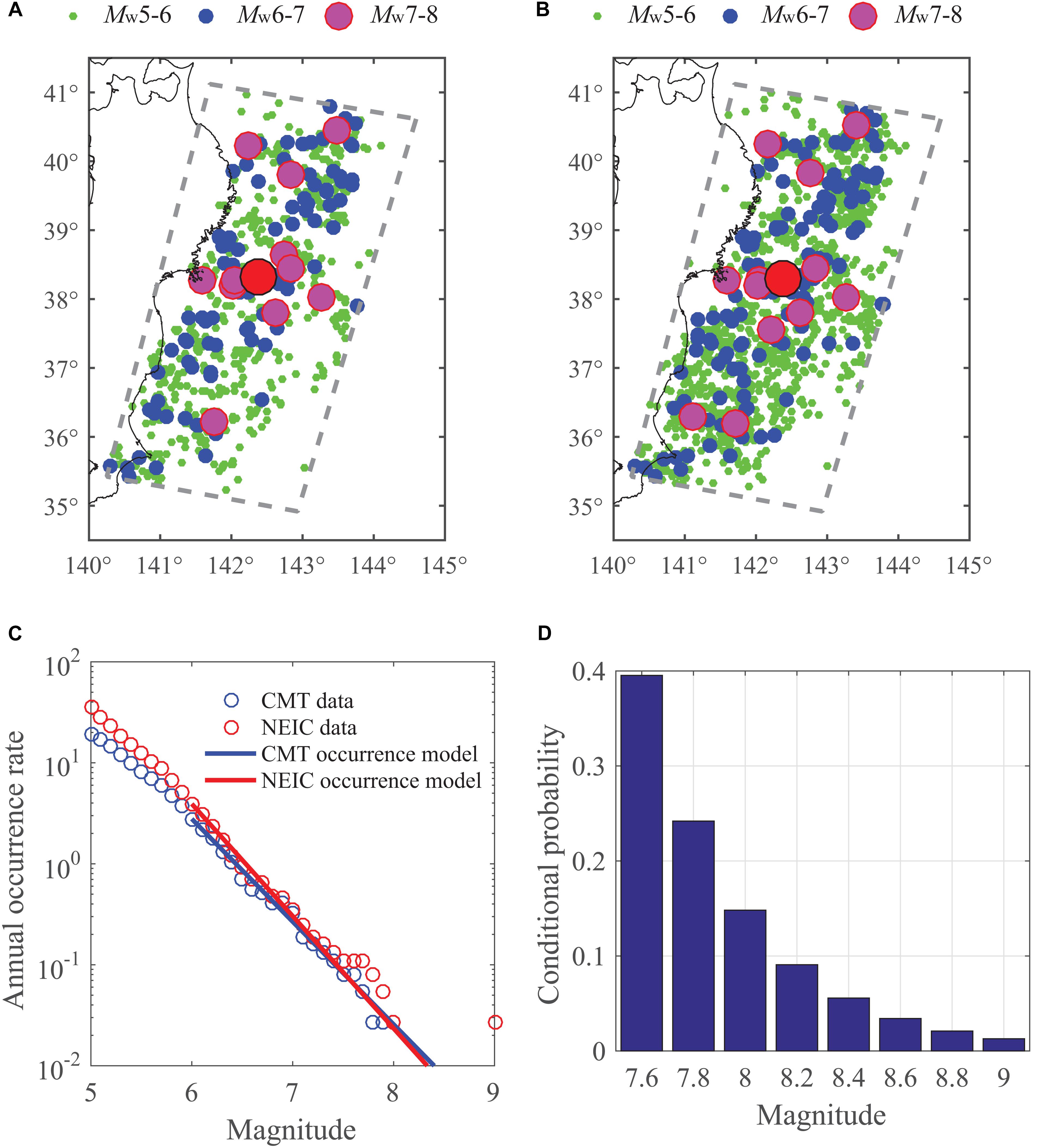
Figure 1. Earthquake source of the off-Tohoku region: (A) Harvard CMT earthquake catalog, (B) NEIC earthquake catalog, (C) Gutenberg-Richter relationships based on the Harvard CMT and the NEIC catalogs, and (D) conditional probability distribution of earthquake magnitudes ≥ M_w 7.5.

Tsunami Modeling

Stochastic Earthquake Source Models

The current state-of-the-practice tsunami hazard maps which are prepared based on the hazard parameters of a single scenario on a single fault cannot deal with potential risks in different situations. A stochastic earthquake slip method for large mega-thrust subduction earthquakes is employed. The uncertainty of earthquake rupture characterization is taken into account by using new scaling relationships and stochastic slip synthesis (Goda et al., 2014, 2016). This is an extension of the earthquake slip modeling method developed by Mai and Beroza (2002) based on the spectral synthesis of random field, which is originally targeted for M_w 6-8 crustal earthquakes. For predictive purposes, the post-event evaluation for relevant source models is not applicable. Therefore, it is reasonable to take into account a wide range of possible slip distributions that are encompassed by the scaling relationships, and to interpret this as epistemic uncertainty. This step of earthquake slip model generation corresponds to f_EQS|Mw in Eq. (1). An example of the earthquake slip model is shown in Figure 2, exhibiting a heterogeneous distribution of earthquake slip over the rupture plane and the large concentration of earthquake slip.

FIGURE 2

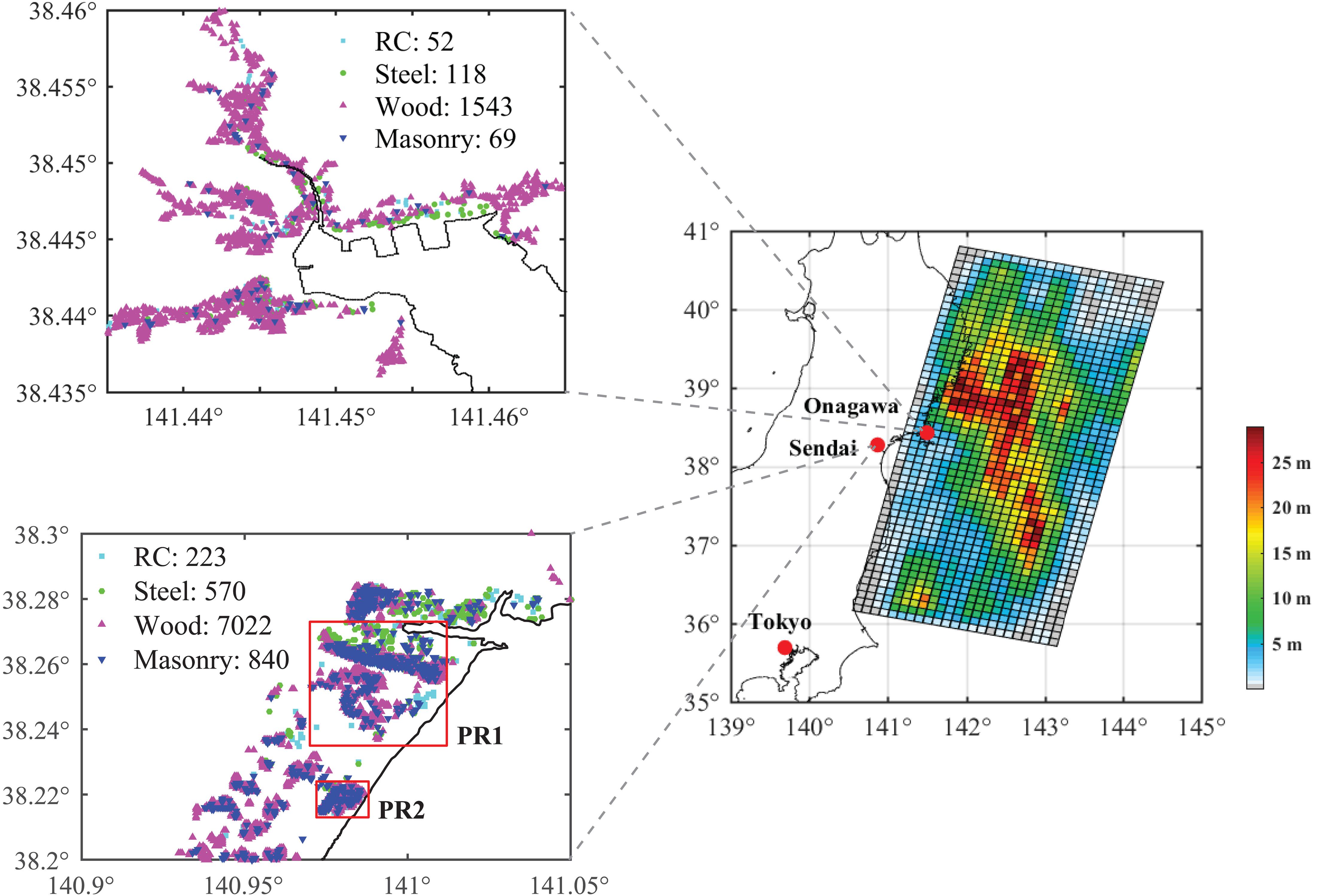
Figure 2. Building portfolios of Sendai and Onagawa. An illustrative earthquake slip model of M_w 9.0 events is displayed in the regional map of Tohoku, Japan.

In light of the 2011 Tohoku tsunami, a seismic source zone, which is sufficiently large to accommodate a M_w 9.0 event, is defined as 650 km along the strike direction and 250 km along the dip direction off the Tohoku region of Japan (Goda et al., 2016). To apply the stochastic synthesis method for generating slip distributions, the fault plane is discretized with sub-faults of 10 km × 10 km which have a constant strike of 193° and variable dip angles gradually steepening from 8° to 16° along the down-dip direction, based on the source model by Satake et al. (2013). The reasons for selecting the Satake et al. (2013) source model as reference are: (i) it gives the best performance among the eleven inverted source models in matching the observed inundation due to the 2011 Tohoku event (Goda et al., 2014), (ii) it was developed using tsunami data and kinematic rupture processes were considered, and (iii) the tsunami simulation codes used in this study and the tsunami computation method adopted by Satake et al. (2013) are similar. The asperity zone corresponds to a smaller sub-region where a set of sub-faults has slip values greater than a threshold value and it is typically two to three times the average slip. The size and location of asperity zones of different magnitudes are different.

The fault rupture (i.e., geometry and slip distribution) is characterized through earthquake source models, multiple earthquake source parameters of which are obtained by applying scaling relationships given the magnitude (Goda et al., 2016). Three types of seismic source parameters are required for the stochastic tsunami simulation: i) geometry parameters including the fault width W, fault length L, and fault area S, ii) slip parameters including the mean slip D_a, maximum slip D_m, and Box-Cox power B, and iii) spatial slip distribution parameters including the correlation lengths along dip and strike directions A_z and A_x, and the Hurst number H.

The first step of stochastic source modeling is to obtain the geometry and key slip parameters (mean and maximum slips). The dimension of the fault plane is determined by the fault width W and length L, which are obtained by the following scaling relationships (Goda et al., 2016):

$${\log }_{10}W=-0.4877+0.3125M_w+0.1464{\mathrm{\epsilon }}_W(5)$$

$${\log }_{10}L=-\mathrm{0.1.5021}+0.4669M_w+0.1717{\mathrm{\epsilon }}_L(6)$$

where the ε terms are regression residuals of the corresponding source parameters. The fault plane is randomly located within the whole pre-defined source region. The equations for D_a and D_m are given below:

$${\log }_{10}{D}_a=-5.7933+0.7420M_w+0.2502{\mathrm{\epsilon }}_{D_a}(7)$$

$${\log }_{10}{D}_m=-4.5761+0.6681M_w+0.2249{\mathrm{\epsilon }}_{D_m}(8)$$

In addition, the heavy right tail feature of the slip distribution (i.e., its positive skewness) is modeled via Box-Cox transformation (Box and Cox, 1964):

$$Y=\frac{X^B-1}{B}(B\ne 0)(9)$$

where B is the Box-Cox power parameter, Y is the transformed slip, and X is the original slip (note: when B=0, Y = log⁡(X)). An optimal Box-Cox parameter can be estimated by evaluating the linear correlation coefficient of the standard normal variable and the transformed variable of the slip values. The slip distribution is further adjusted to achieve a target mean slip D_a and a maximum slip D_m to avoid very large slip values exceeding the target maximum slip.

Secondly, the spatial characteristics of the power spectra are expressed as wave-number spectra in down-dip and along-strike directions. The wave number spectra are based on a von Karman auto-correlation function:

$$P(k)\propto \frac{A_x{A}_z}{{(1+k^2)}^{H+1}}(10)$$

A_x and A_z control the absolute level of the power spectrum in the low wave-number range (i.e., k≪1) and capture the anisotropic spectral features of the slip distribution. H is the Hurst number, which determines the slope of the power spectral decay in the high wave-number range and is theoretically constrained to fall between 0 and 1. It is given a value of 0.99 with a probability of 0.43 and a sampled value from the normal distribution with mean of 0.714 and a standard deviation of 0.172 with a probability of 0.27 (Goda et al., 2016). A_x and A_z are determined by:

$${\log }_{10}{A}_x=-1.9844+0.4520M_w+0.2204{\mathrm{\epsilon }}_{A_x}(11)$$

$${\log }_{10}{A}_z=-1.0644+0.3039M_w+0.1592{\mathrm{\epsilon }}_{A_z}(12)$$

Subsequently, multiple realizations of slip distributions with desired stochastic properties are generated using a Fourier integral method (Pardo-Igúzquiza and Chica-Olmo, 1993). The amplitude spectrum of the target slip distribution is specified by the theoretical power spectrum with the estimated correlation lengths and Hurst number, while the phase spectrum is represented by a random phase matrix. The constructed complex Fourier coefficients are transformed into the spatial domain via 2D inverse Fast Fourier Transform (FFT). The synthesized slip distribution is converted via Box–Cox transformation to achieve realistic heavy right-tail features of the slip distribution. An acceptable slip distribution is expected to have its maximum slip patch and similar slip concentration within the asperity zone of the original distribution. The regression residuals of six source parameters (i.e., W, L, D_a, D_m, A_x, and A_z) are distributed according to a multivariate normal distribution; more details can be found in Goda et al. (2016).

Tsunami Inundation and Propagation

Tsunami modeling is carried out using a well-tested numerical code (Goto et al., 1997) which is capable of generating off-shore tsunami propagation and inundation profiles by evaluating non-linear shallow water equations with run-up using a leap-frog staggered-grid finite difference scheme. The run-up calculation is performed by a moving boundary approach, where a dry or wet condition of a computational cell is determined by comparing the total water depth with its elevation. A complete set of bathymetry/elevation data, surface roughness data and coastal/riverside structures (e.g., breakwater and levees) is obtained from the Miyagi Prefecture Government. The bathymetry and elevation data are provided in five grid resolutions: 1350-m, 450-m, 150-m, 50-m, and 10-m. The ocean bathymetry data are based on the 1:50,000 bathymetric charts and digital database developed by the Japan Hydrographic Association from the nautical charts developed by the Japan Coastal Guard. The land elevation data are included in the DEM developed by the Geospatial Information Authority of Japan and the raw elevation data were obtained from airborne laser surveys and aerial photographic surveys. The measurement errors of the data are less than 1.0 m horizontally and 0.3–0.7 m vertically (as standard deviation). The elevation data of the coastal/riverside structures with dimensions less than 10 m are provided by municipalities in Miyagi Prefecture, because those with dimensions larger than 10 m are included in the DEM data. In tsunami simulations, the coastal/riverside structures are represented by a vertical wall at one or two sides of the computational cells. To evaluate the volume of water that overpasses these walls, Homma’s overflowing formulae are employed.

In tsunami simulation, the initial water surface elevation is evaluated based on formulae by Okada (1985) and Tanioka and Satake (1996). The latter equation accounts for the effects of horizontal sea-floor movements in case of steep sea-floor, inducing additional vertical water dislocation. Although the sea-floor deformations are obtained for the same event, spatial characteristics of the sea-floor displacements vary significantly among the models, leading to different tsunami wave profiles at various locations along the Tohoku coast (Goda et al., 2014). The fault rupture is assumed to occur instantaneously, and numerical tsunami calculation is performed for duration of 2 h. The tidal fluctuation is not taken into account in this study. The tsunami flow resistance is parametrized by Manning’s roughness coefficient in the shallow water equations. The bottom friction is evaluated through Manning’s formula according to the national land use standard in Japan by considering six types of land use. The assigned roughness coefficients are a crude representation of the actual situation and depend on the resolution of the available DEM. Consequently, a more detailed roughness condition is applied when a DEM of finer resolution is used, which gives more reliable tsunami intensity measure prediction (Kaiser et al., 2011; Griffin et al., 2015). Although the actual surface roughness is influenced by multiple factors (e.g., building density and slope) and thus the friction may be spatially variable within the same type of land use, a constant Manning’s roughness coefficient is applied for each type of land use since the influence of surface roughness is not the main focus of this study.

Tsunami Loss Estimation

Tsunami damage and loss are calculated using fragility models developed by De Risi et al. (2017), which are based on the damage data of the 2011 Tohoku event. Integrated with simulated tsunami intensities, for mutually exclusive damage states that are defined in a discrete manner, the damage probability p(ds_i|im) of damage state ds_i can be obtained given the IM of a building, which can be expressed as:

$$p(d{s}_i|im)=p(DS\ge d{s}_i|im)-p(DS\ge d{s}_{i+1}|im)(13)$$

By incorporating damage cost models for different buildings, the tsunami damage information can be transformed into tsunami loss information for individual buildings as well as building portfolios. The loss ratio, denoted by R_L(ds), represents the percentage of replacement cost of a building for a given ds. In this study, a uniform damage ratio scheme is applied to account for the uncertainty in damage cost, which is assigned as: 0.0 for DS1 (no damage), 0.03–0.1 for DS2 (minor), 0.1–0.3 for DS3 (moderate), 0.3–0.5 for DS4 (major), 0.5–1.0 for DS5 (complete), and 1.0 for DS6 (collapse and washed-away). The lower and upper bounds of the assumed damage ratio ranges are consistent with a tsunami damage assessment procedure by the Ministry of Land Infrastructure and Transportation of Japanese Government, where representative damage ratios of 0.0, 0.05, 0.2, 0.4, 0.6, and 1.0 are suggested for DS1, DS2, DS3, DS4, DS5, and DS6, respectively. Using the damage state probability p(ds) and the loss ratio R_L(ds), tsunami damage cost for a given tsunami hazard intensity can be calculated as:

$$L=C_R\sum _{i=1}^{6}p(d{s}_i)\times R_L(d{s}_i)(14)$$

where C_R is the replacement cost of a building. An advantage of using loss metrics, instead of damage probability or the number of damaged buildings, is that the consequences due to tsunami damage in coastal cities/towns can be aggregated for the entire building portfolio. Moreover, calculated values of tsunami damage probability can be used in Monte Carlo sampling to generate realizations of individual damage states for the buildings. This re-sampling facilitates the development of exceedance probability (EP) curves which are the fundamental information to achieve various tsunami risk metrics, such as annual average loss (AAL) and value at risk (VaR).

Tsunami Insurance Rate-Making

Insurance premium is composed of pure premium P_pure, risk premium P_risk, and transaction fees P_expense (Kuzak and Larsen, 2005; Gray and Pitts, 2012):

$$P_{premiuim}=P_{pure}+P_{risk}+P_{expense}(15)$$

The risk premium is determined by the pure premium and various risk factors for insurers (e.g., insurers’ capital reserve, transaction fees, and rate regularity requirement). The transaction fees reflect the administrative costs involved in issuing the insurance policy, which include marketing, premium taxes, and processing fees. P_risk, and P_expense are not negligible but are difficult to evaluate. In this study, pure premium is focused upon because it is the most essential component and its quantification relies on tsunami risk assessment. P_pure is calculated as AAL based on an EP curve. In the stochastic tsunami loss estimation method, tsunami loss events over a specified period are obtained and thus AAL can be evaluated as the sum of the simulated losses divided by the total duration of the simulation period.

The incurred loss for the insurer, which is also the claims paid to the policyholders, is determined by the arrangements of three insurance parameters for risk transfer: deductible D, limit/cap C, and co-insurance factor η. The payout I_P of an insurance policy is commonly expressed as:

$$I_P(L)=\{\begin{array}{cc}0\mathit{\hspace{1em}}\hfill & L\le D\hfill \\ \mathrm{\eta }(L-D)\mathit{\hspace{1em}}\hfill & D<L<C\hfill \\ \mathrm{\eta }(C-D)\mathit{\hspace{1em}}\hfill & L\ge C\hfill \end{array}(16)$$

According to the General Insurance Rating Organization of Japan³, the earthquake insurance policy in Japan only covers building damage and loss experiencing inundation depth higher than 45 cm for tsunami loss. Therefore, an inundation depth less than 45 cm is considered to cause no insurance loss for tsunamis. The value of the insured property is limited to the market value, and thus for typical wood houses, the limit is set to 208,000 USD taking the mean replacement cost as the market value. The coinsurance factor is assumed to be 1.

Building Portfolio

The building portfolios of Sendai and Onagawa are focused upon in this study, as shown in Figure 2. These two locations are selected because Sendai is located on a plain coast, while Onagawa is located on a ria coast. A building portfolio in Sendai consists of 223 RC structures, 570 steel structures, 7,022 wood structures, and 840 masonry structures. A building portfolio in Onagawa contains 52 RC, 118 steel, 1,543 wood, and 69 masonry structures.

Sendai is on a plain coast and the elevation rises gradually. Within 2 km from the sea, the elevation is generally below 3 m. Many buildings in Sendai are at elevations between 1 m to 3 m. To visualize the spatial tsunami hazard variation, two smaller regions PR1 and PR2 in Sendai are selected. There are 3,679 buildings in PR1, containing 89 RC, 316 steel, 2,920 wood, and 354 masonry structures, whereas there are 1,070 buildings in region PR2, including 27 RC, 17 steel, 911 wood, and 115 masonry structures. These two small regions have a concentration of buildings, and structures in PR1 have different distances from the sea while the buildings in PR2 is located within 1 km from the coastline. The elevation maps for PR1 are shown in Figure 3 to display the differences caused by DEM resolutions. Because the coastal area of Sendai is relatively low and flat, the elevation range shown in Figure 3 is limited to 8 m to focus on the variation in the lower elevations. The coarse resolution tends to reduce the spatial variation in elevation, particularly for places with abrupt changes of elevation. For example, there is a red patch at the top of the 10-m map with elevations higher than 8 m, while the 150-m and 450-m maps fail to reflect this accurately. The high-elevation area at the top of the 10-m map is completely missed out in the 450-m map. In other words, the assignment of coarse elevation results in loss of accuracy with the decrease in resolution. Four specific locations at 2 m elevation with different distances from the coastline (i.e., P1 of 0.5 km, P2 of 1.2 km, P3 of 1.5 km, and P4 of 2 km) are selected to examine the differences in local tsunami risk caused by DEM resolution. In the 10-m map, the elevations of these four locations are similar, which are around 2 m above the mean sea level, while the corresponding elevations given by the coarser DEMs are different from this value, as shown in Table 1. The elevations of P3 given by the 150-m DEM and those of P3 and P4 given by the 450-m DEM indicate substantial errors although the elevations at other locations do not show such discrepancy. The finer 50-m resolution gives a better estimation for all four locations than the 150-m and 450-m maps, although the elevation at P1 is still more than 50% higher than that of 10-m resolution.

FIGURE 3

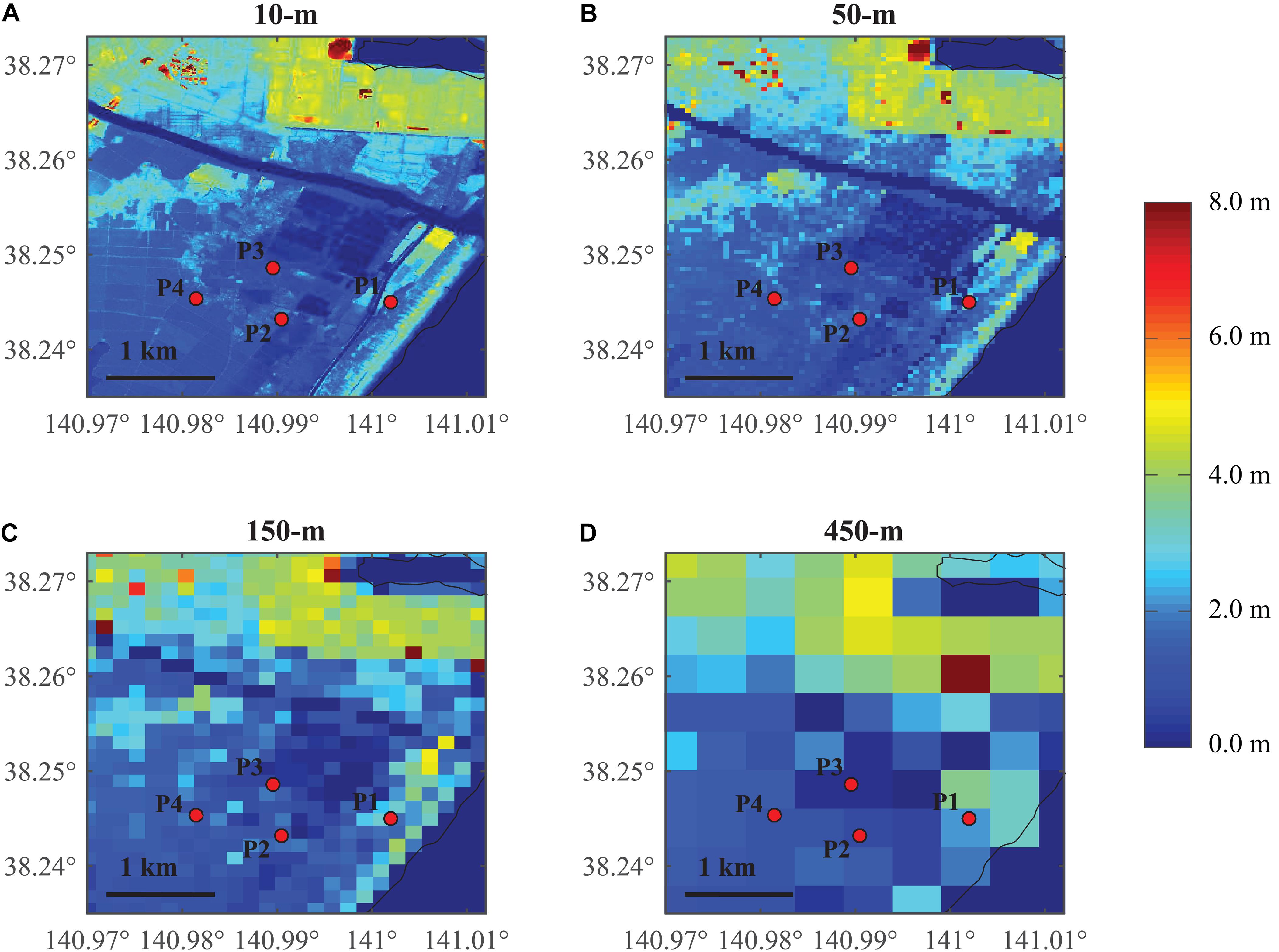
Figure 3. Elevation maps for region PR1 in Sendai of different resolutions: (A) 10-m, (B) 50-m, (C) 150-m, and (D) 450-m.

TABLE 1

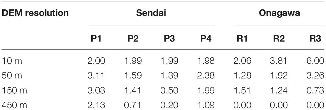
Table 1. Elevations of chosen locations using DEMs of different resolutions (m).

In Onagawa, buildings are surrounded by steep hills/mountains and the sea and concentrated in a small flat area close to the coast and the elevation rises rapidly toward inland (Figure 4). The majority of buildings in Onagawa are located within 1 km from the coastline, and about a half are located within 0.3 km from the sea. Similarly, three locations R1, R2, and R3 in Onagawa are selected to reflect the differences caused by DEM resolution. The locations R1, R2, and R3 are fairly close with a similar distance of about 300 m from the sea, but have different elevations which are about 2 m, 4 m, and 6 m, respectively, according to the 10-m DEM (Figure 4). The elevations assigned to these three locations based on different DEMs are summarized in Table 1. Although the 50-m DEM has the second finest resolution, it still cannot capture the realistic elevations at R2 and R3, giving 1.92 m for R2 and 3.26 m for R3. Even worse accuracy of local elevation is resulted from the 150-m and 450-m DEMs. Particularly, the 450-m resolution cannot provide elevations close to realistic values for any of the three locations. The 450-m DEM is regarded as unsuitable for representing topographic features of Onagawa realistically, which made the three locations below the mean sea level. The 50-m and 150-m DEMs still show the changes of elevation but are not well resolved to distinguish different elevations within small areas. The 50-m DEM, which is acceptable to represent elevations for Sendai, is not suitable and assigns inaccurate elevations to all three locations. With the increase of grid size, the assigned elevations tend to become lower.

FIGURE 4

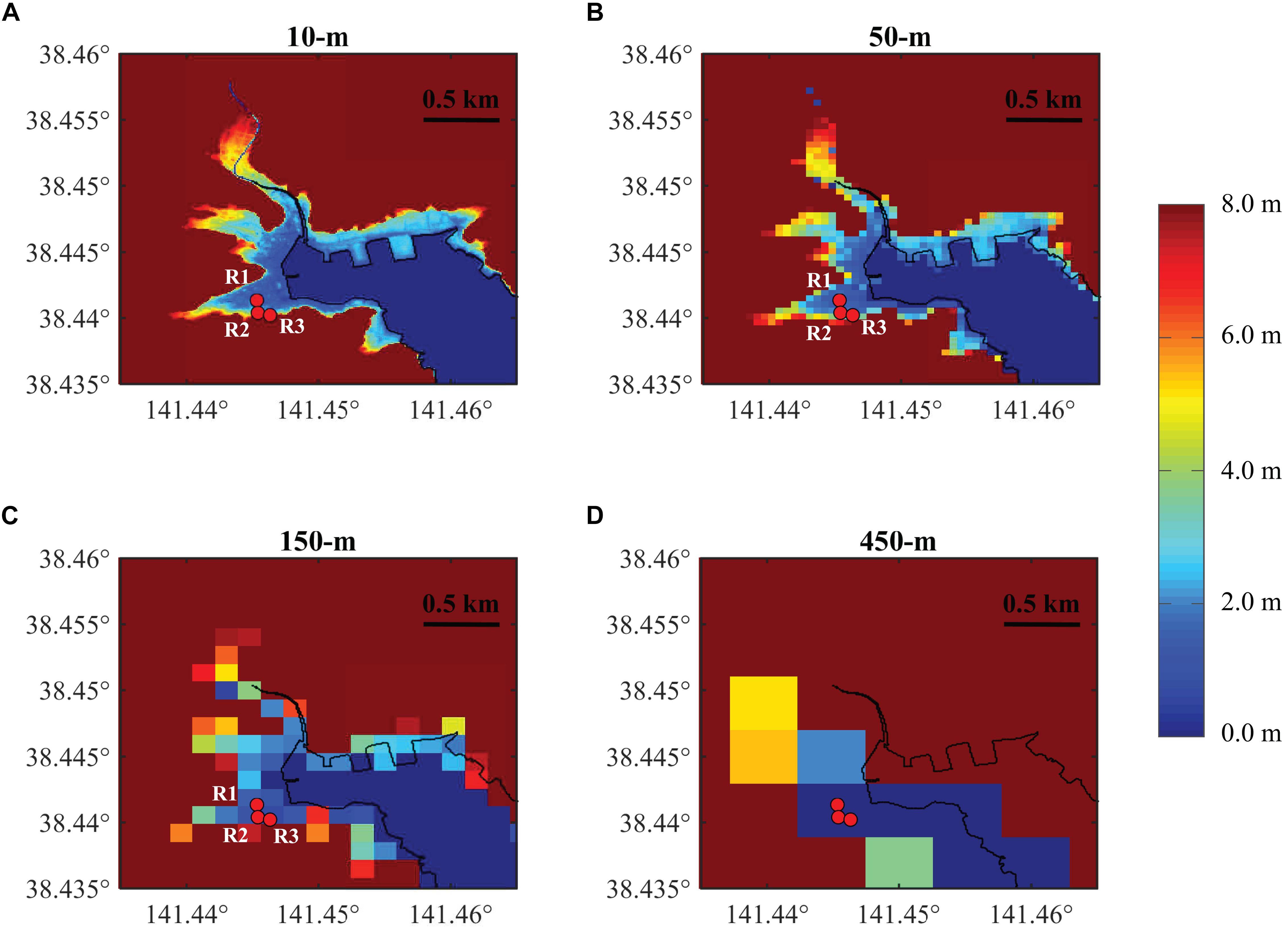
Figure 4. Elevation maps for region RR1 in Onagawa of different resolutions: (A) 10-m, (B) 50-m, (C) 150-m, and (D) 450-m.

Influence of Elevation Data Resolution on Tsunami Loss Estimation

Plain Coast

Tsunami Hazard

To identify critical tsunami loss scenarios, three earthquake slip distributions are chosen from 300 stochastic source models for M_w 9.0 events, by ranking the total tsunami loss of Sendai based on the 10-m DEM, noting that the M_w 9.0 events have the highest contribution to total tsunami loss. The earthquake slip models are shown in Figure 5. The selected loss scenarios aim to show the median case (i.e., 50th percentile) and the rare cases (i.e., 10th and 90th percentiles). In other words, the loss scenarios 1 to 3 correspond to the model which gives tsunami loss ranked 10th percentile, 50th percentile, and 90th percentile, respectively. The inundation maps for PR1 based on four resolutions of DEM are shown in Figure 6, given the three slip models. For each loss scenario, the slip model is the same, while the losses are affected by different resolutions of the DEMs. Because of the variation in tsunami inundation caused by the DEM resolution, the same slip models do not necessarily result in the same rank of tsunami loss at different resolutions, and it is mainly intended to demonstrate the variation at different inundation scales.

FIGURE 5

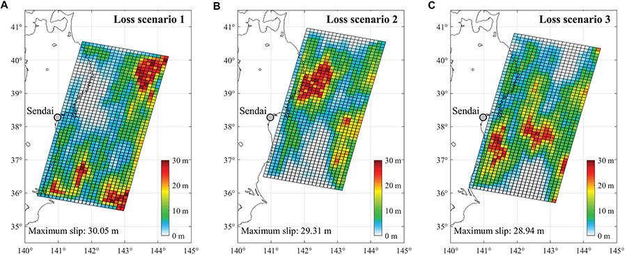
Figure 5. Earthquake slip models of M_w 9.0 events corresponding to three loss scenarios identified for Sendai: (A) loss scenario 1 (10th percentile of total loss), (B) loss scenario 2 (50th percentile of total loss), and (C) loss scenario 3 (90th percentile of total loss).

FIGURE 6

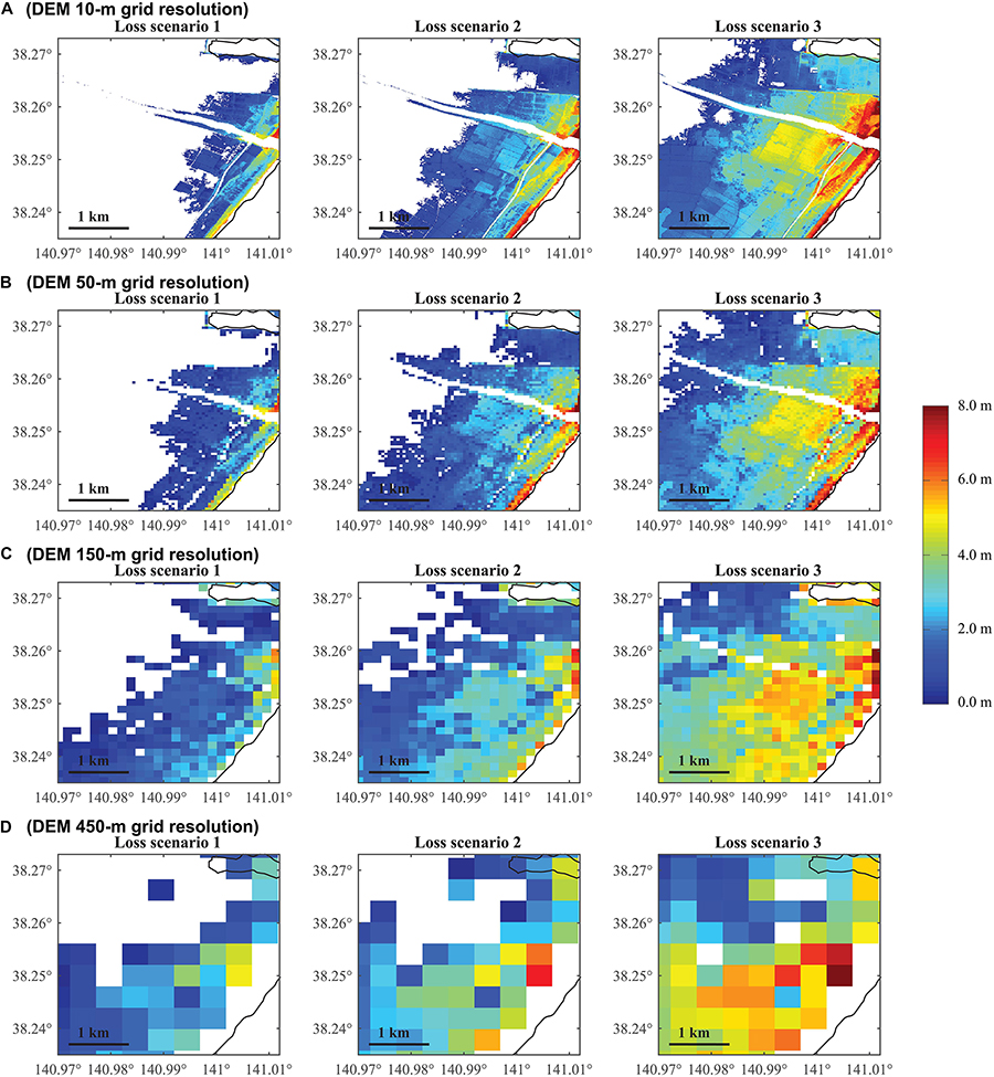
Figure 6. Inundation depth maps of M_w 9.0 events for region PR1 in Sendai by considering different DEM resolutions: (A) 10-m, (B) 50-m, (C) 150-m, and (D) 450-m.

Generally, a coarser DEM is less capable of reflecting the variation of inundation depth locally and thus makes the inundation depth more uniform at a local scale, as shown in Figure 6. For example, there is a strip of area along the coastline with the highest tsunami depth, and the maximum inundation depth becomes higher than 6 m for the loss scenario 3 of 10-m resolution. This red-colored area gradually starts to disappear as the resolution becomes coarser from 10 m to 450 m. The 50-m DEM is more capable of capturing the spatial variation of inundation depth than the 150-m and 450-m DEMs, but sill loses the detail in abrupt changes of inundation depth. For the 10-m resolution, the inundation depth decreases rapidly with increasing distance from the coastline, while with the increase in grid size, the decrease of tsunami intensity becomes more gradual spatially. On the other hand, a coarser resolution tends to underestimate the tsunami intensity for areas right beside the coast while tends to overestimate the hazard for areas at the far end of the inundated area. It can be seen that the places of the highest tsunami intensity of 50-m, 150-m, and 450-m resolution are not consistent with those of 10-m resolution. In other words, a coarse DEM may not be able to capture the spatial variability of tsunami intensity accurately. The coarse resolutions are unable to evaluate (locally) high inundation depths accurately, and they tend to result in larger inundation areas. The inundation results based on the 450-m resolution data are highly inconsistent with those based on finer resolutions in terms of inundation amplitude, spatial distribution, and inundation area.

Tsunami Loss

Given the stochastic inundation depths for the building portfolio in Sendai, the annual EP curves for tsunami loss are shown in Figure 7 for the whole Sendai, PR1, and PR2. The EP curves are obtained based on 2,400 stochastic slip models (i.e., eight magnitude ranges and 300 slip models per magnitude range). It is noted that the 450-m DEM results in negative values of elevations for a large number of buildings close to the coast, which means those buildings are located below the mean sea level although not true in reality. In tsunami loss calculations, the elevations of those buildings are set to 0. Consequently, this modification reduces the differences of tsunami loss at different locations. For example, if elevations of 1 m and −5 m are assigned to two buildings A and B based on the 450-m DEM, assuming they experience the same inundation height, there would be a difference of 6 m in inundation depth but the difference is reduced to only 1 m if −5 m is corrected to zero. These errors are due to the inappropriateness of the 450-m DEM in assigning accurate elevations.

FIGURE 7

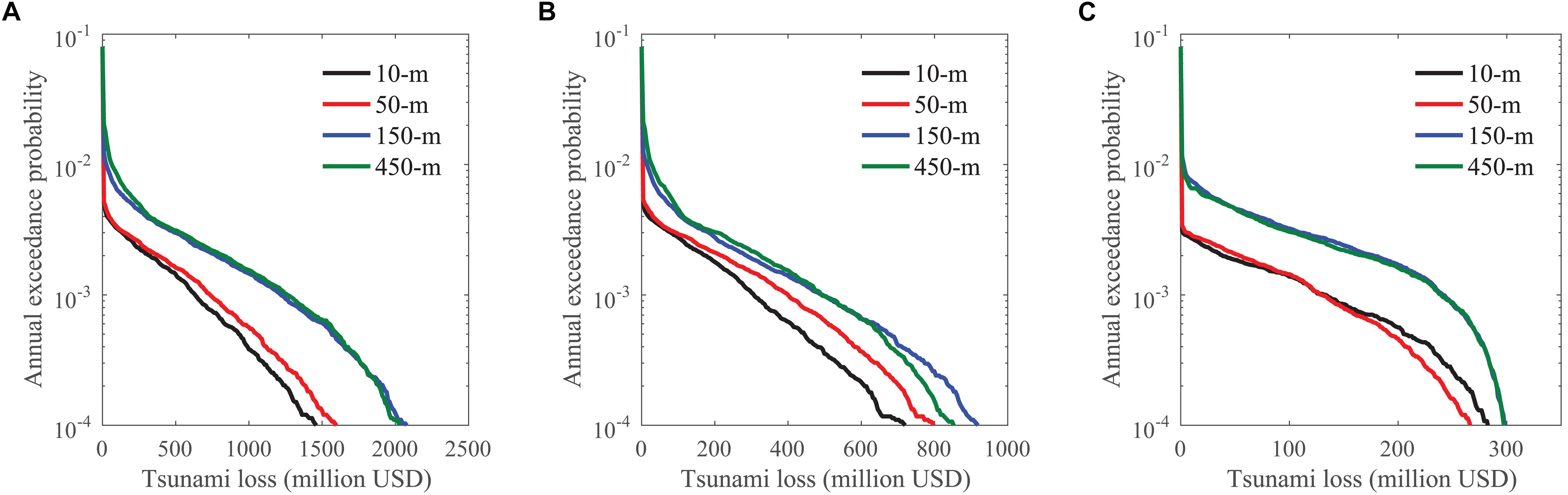
Figure 7. Tsunami loss curves in Sendai: (A) whole Sendai, (B) PR1, and (C) PR2.

From the results, the 150-m and 450-m DEM cases lead to more than 30% higher tsunami losses, especially for more frequent events. For the whole Sendai, the 10-m resolution case results in the smallest estimated loss, followed by the 50-m, 150-m, and 450-m resolution cases. The 10-m and 50-m resolution cases are similar in terms of total tsunami loss. One of the risk metrics to assess the risk at a certain probability level is VaR, which is the risk value at a selected probability level. The VaR_0.999 for the 10-m resolution case is about 700 million USD, while that for the 150-m resolution case is about 1,500 million USD, which is almost twice as large as that of the 10-m resolution case. The comparisons of the tsunami loss distributions and the corresponding risk metrics for different grid resolution cases highlight the importance of the elevation data resolution to the accurate estimation of the potential financial impact due to catastrophic tsunamis.

A coarser DEM tends to underestimate the tsunami hazard closer to the sea and overestimate it at farther places. Therefore, the resulted difference in total tsunami loss from different DEM resolutions depends on the spatial distribution of buildings as well. For example, the difference between the case of 10-m and 150-m/450-m case is greater for the whole Sendai than PR1. This is because the whole Sendai includes more buildings farther from the coast which are inundated for the cases of 150-m and 450-m resolution, but not inundated for the cases of 10-m and 50-m resolution. VaR_0.999 for the 150-m resolution case is reduced to about 40% higher than that of 10-m resolution. The tsunami loss for the 150-m resolution case is similar to that for the 450-m resolution for more frequent events but is lower for extreme events with longer return periods. As seen in Figure 6, the 450-m DEM case leads to some areas not inundated but are inundated in the 150-m inundation maps. For PR2 which has a smaller area size and is closer to the sea, the tsunami losses for the 150-m and 450-m resolution cases are dramatically higher than those for the 10-m and 50-m resolution cases due to the overall overestimation of inundation depth based on the 150-m and 450-m DEMs, particularly for areas farther from the coast. Although the differences of VaR_0.9999 are within 20%, VaR_0.999 for the 150-m and 450-m resolution cases are almost twice as large as that for the 10-m resolution case.

As seen in the tsunami hazard maps for different DEM resolutions, how the tsunami intensity is weakened when waves traveling inland is significantly affected by DEM resolution. In Sendai, with low-lying flat topography, an increasing distance from the coast reduces the tsunami hazard level, however, the coarse DEM is less capable of reflecting the difference. To investigate such effects, the tsunami loss curves of a single structure at P1, P2, P3, and P4 in PR1 are compared in Figure 8 by distinguishing different DEM resolution cases and structural types. These locations all have an elevation of around 2 m (Table 1) and have increasing distances from the coast, which are roughly 0.5 km, 1.2 km, 1.5 km, and 2 km. The corresponding inundation depth distributions from the 300 simulations of the M_w 9.0 events are shown in Figure 9, noting that the M_w 9.0 events have the highest contribution to total tsunami loss. Although it has been found in Figure 7 that tsunami loss for the 50-m resolution case is relatively close to that for the 10-m resolution case, the estimated local risks at P1 for the two resolution cases are different. Around P1, a rapid change of elevation occurs, which makes the coarser DEMs likely to assign an erroneous elevation. The 50-m DEM assigns an elevation more than 3 m to P1. In the 10-m elevation map, P1 is located in the front of an area with increased elevation, while in the 50-m elevation map P1 is located at the farther side of the area with an increase of elevation due to the reduced resolution. Consequently, for the 10-m case tsunami waves are weakened after arriving at P1 due to a sudden increase of elevation, while for the 50-m case the wave height has been reduced before arriving P1. Compared to the 10-m resolution case, which is taken as the most reliable case, more than 80% of the depths given by the 50-m DEM are less than 2 m and no depth is greater than 5 m, while using the 10-m DEM more than a half of the depths are higher than 4 m. As seen in Figure 6 the inundation depths in the 50-m maps are lower than those in the 10-m maps before tsunami waves arrive at P1. Furthermore, with a higher elevation given by the 50-m case, consequently the inundation intensity at P1 estimated by the 50-m DEM is significantly lower than that by the 10-m DEM. Although the 150-m and 450-m resolution cases do not generate depths higher than 7 m as the 10-m resolution case does, there are more cases where depths between 2 and 6 m occur, compared with the 10-m resolution case. This eventually makes the tsunami loss curves at P1 similar for the 10-m, 150-m, and 450-m resolution cases.

FIGURE 8

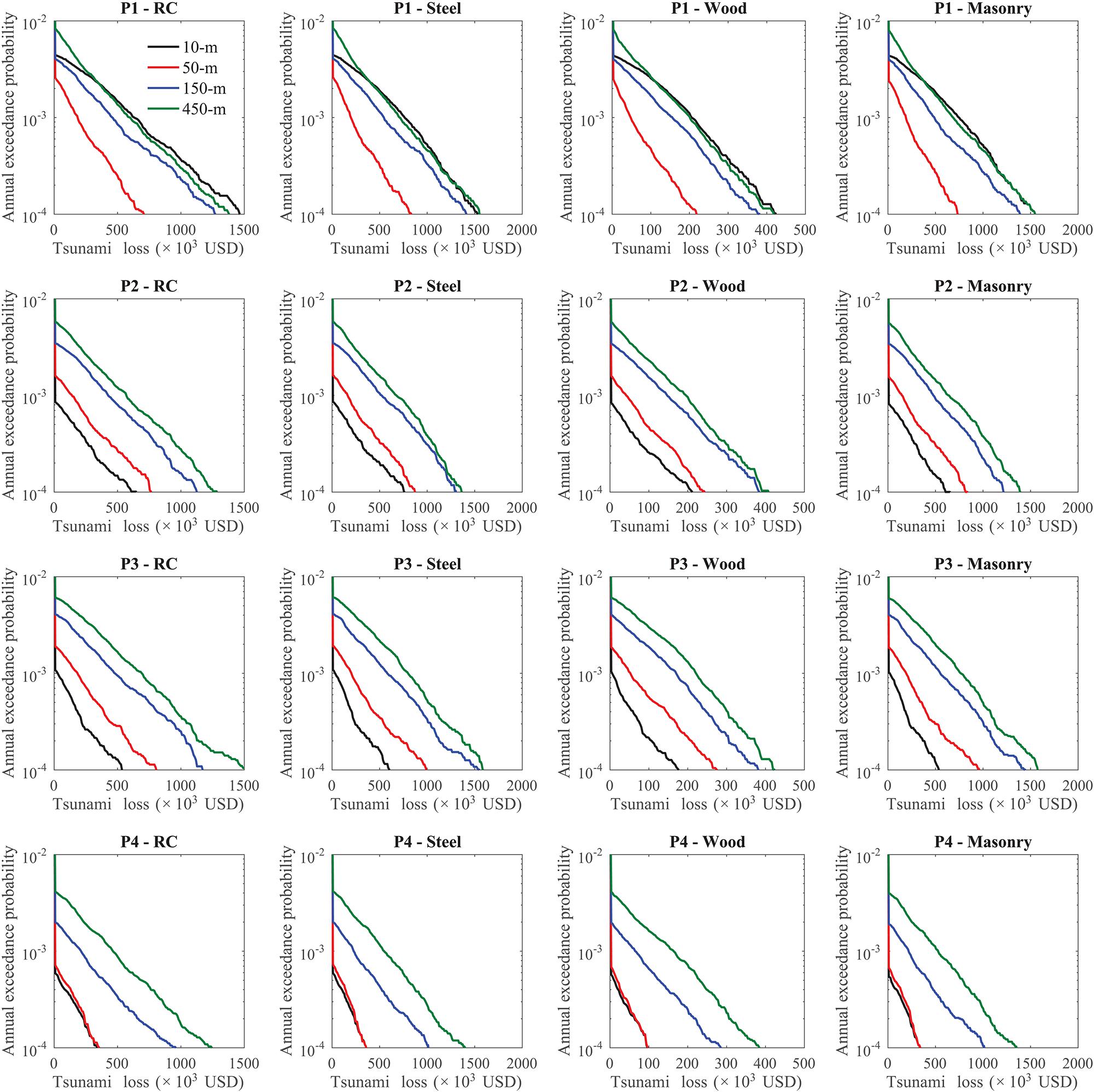
Figure 8. Tsunami loss EP curves at different locations in Sendai.

FIGURE 9

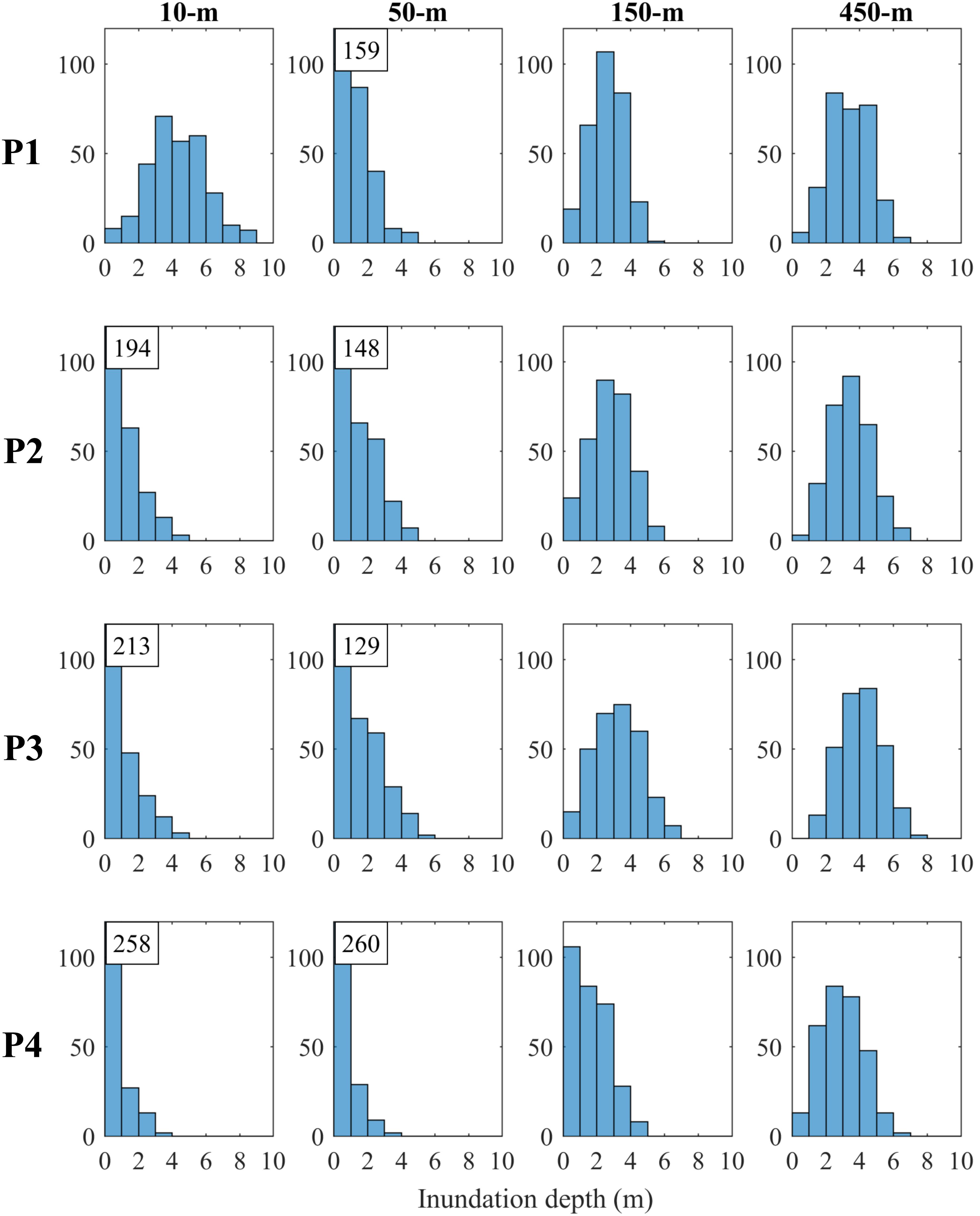
Figure 9. Inundation depth distribution at four locations in Sendai for the M_w 9.0 events by considering different DEM resolutions (The counts exceeding the y axis limit are indicated in a box). The histogram in each subfigure panel is based on 300 stochastic slip models.

For other three locations, where the elevations given by the 50-m DEM are relatively close to that for the 10-m resolution case, the tsunami loss curves for P4 at the 50-m resolution are similar to the 10-m resolution case but higher for P2 and P3 due to lower elevations assigned by the 50-m DEM. It can be seen in Figure 9 that the 150-m and 450-m resolution cases significantly overestimate the inundation depths at P2, P3, and P4. The tsunami losses at P2 for the 150-m and 450-m resolution cases are twice as large as that of the 10-m resolution case. It is interesting to notice that although the loss curves for the 150 m and 450 m resolution cases are similar at P2, the elevation based on the 150-m DEM is 1.41 m, while that based on the 450-m DEM is only 0.71 m (Table 1). It implies that local risk is affected not only by the assigned elevation but also by other factors. Consequently, for some cases, it would be difficult to determine the relative tsunami risk solely from elevations without conducting tsunami simulations. The differences of the loss curves between finer resolution and coarser resolution cases increase at P3 and P4. This indicates that for local tsunami risk assessment at a particular location, using the 150-m and 450-m DEM can be highly unreliable. The elevations of P3 based on the 150-m and 450-m DEMs are only 0.50 m and 0.20 m, respectively, and thus the loss results are almost three times greater than those for the 10-m resolution case. At P4, the tsunami losses for the 150-m and 450-m resolution cases are significantly higher than the other two cases. The risk decreases significantly from P1 to P4 with tsunami loss curves for the 10-m DEM, but for the 150-m and 450-m resolution cases, the differences between risks at four locations are substantially small.

Ria Coast

Tsunami Hazard

The unrealistic representation of elevation using coarser DEMs results in substantially inaccurate spatial distribution of tsunami intensity measures. The slip models that correspond to the loss scenarios 1 to 3 are shown in Figure 10. The inundation depth maps are shown in Figure 11, by considering three loss scenarios. The loss scenarios are selected by ranking the tsunami loss of 300 M_w 9.0 tsunami simulations for Onagawa using the 10-m DEM, and thus they are not the same slip models for Sendai (Figure 5). Increase in inundation depth and flow velocity can be observed for the different loss scenarios. Although the 50-m DEM case can broadly capture the inundation area, the spatial extent of inundation is visually smaller. Besides, the 50-m DEM case cannot account for the change of tsunami intensity at places near steep hills/slopes. The 150-m and 450-m DEMs do not generate realistic tsunami simulation results for Onagawa. More specifically, the 150-m DEM is not capable of obtaining neither the correct inundated area nor the correct tsunami intensity, whereas the 450-m DEM can hardly capture the reasonable inundated areas, with flooded areas which should not be inundated and the unflooded areas which should be inundated. Besides, some areas turned out to be unflooded for the 450-m resolution case because they are below the mean sea level according to the 450-m elevation data.

FIGURE 10

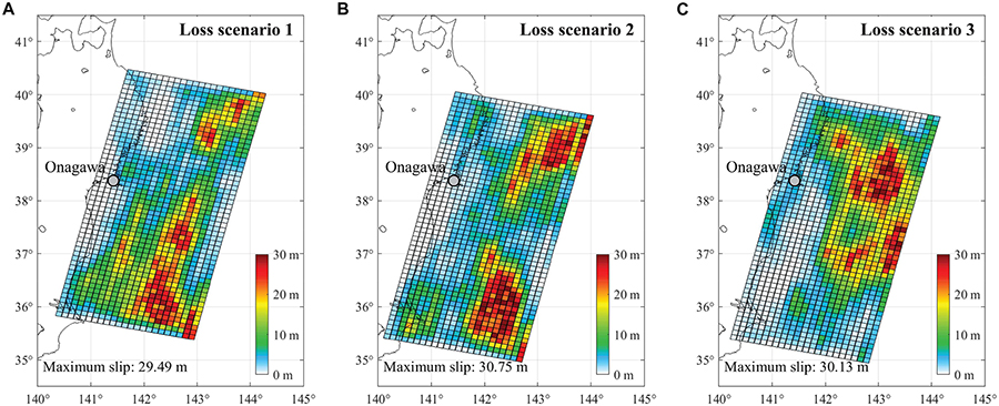
Figure 10. Earthquake slip models of M_w 9.0 events corresponding to three loss scenarios identified for Onagawa: (A) loss scenario 1 (10th percentile of total loss), (B) loss scenario 2 (50th percentile of total loss), and (C) loss scenario 3 (90th percentile of total loss).

FIGURE 11

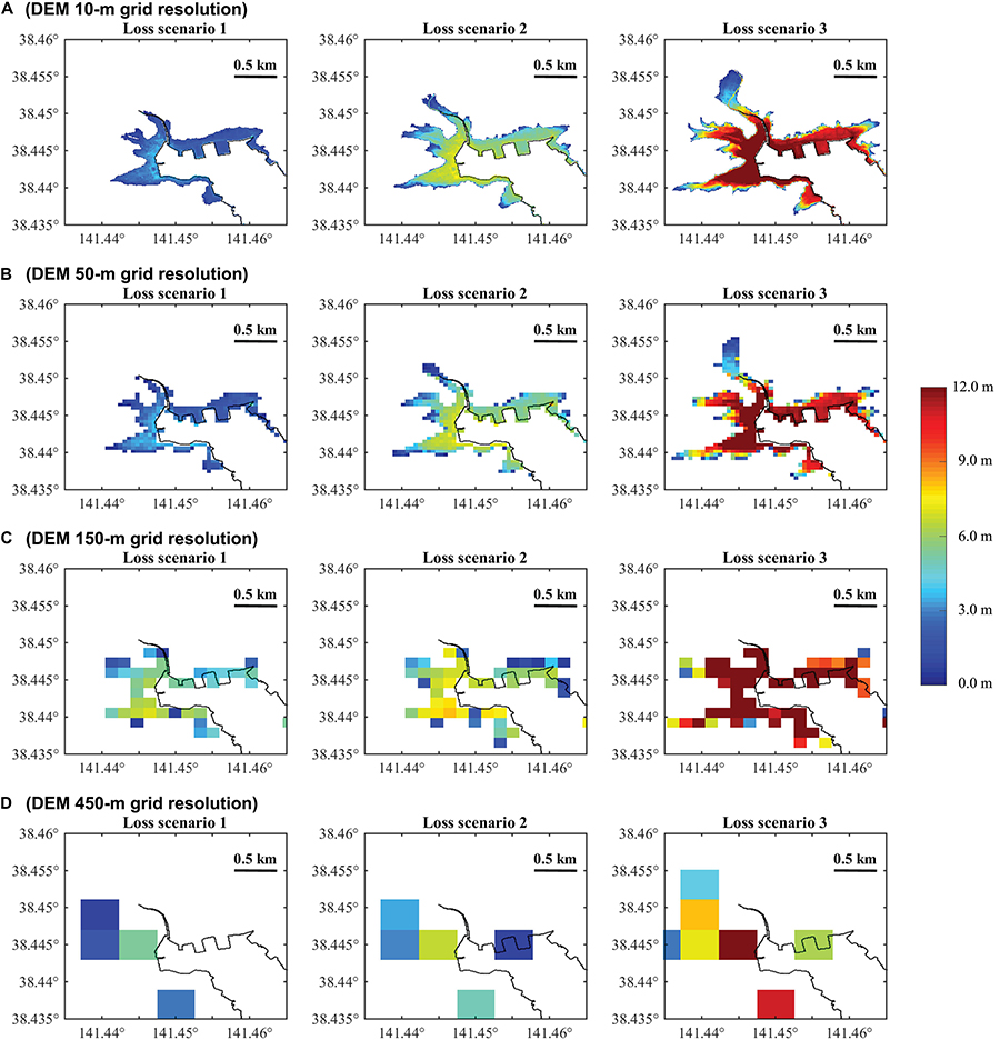
Figure 11. Inundation depth maps of M_w 9.0 events for Onagawa by considering different DEM resolutions: (A) 10-m, (B) 50-m, (C) 150-m, and (D) 450-m.

Tsunami Loss

The total tsunami loss curves for Onagawa are shown in Figure 12 by considering DEMs of different resolutions. The EP curves are obtained based on 2,400 stochastic slip models (i.e., eight magnitude ranges and 300 slip models per magnitude range). The loss curve of the 50-m resolution case is close to the loss curve of the 10-m resolution case but is about 10% lower for the extreme cases. The loss results based on the 150-m and 450-m resolution cases are judged to be unreliable, generating significantly higher losses for the low-inundation scenarios while underestimating losses for the catastrophic events. In terms of regional losses, the 10-m and 50-m DEMs can be used, while the 150-m and 450-m DEMs cannot be relied on.

FIGURE 12

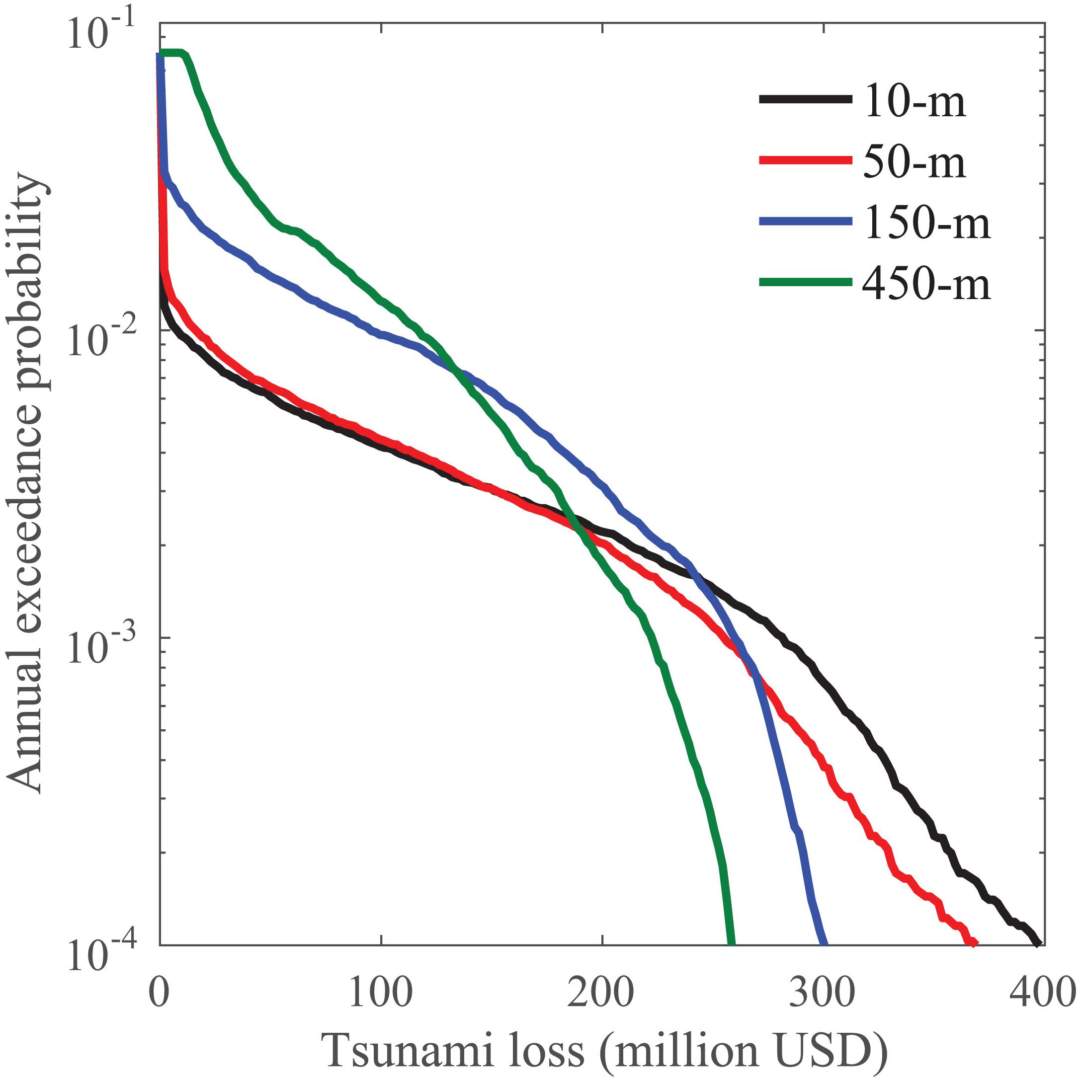
Figure 12. Tsunami loss curves for Onagawa.

The local tsunami risks at R1, R2, and R3 are consistent with the assigned elevations in Table 1. It can be seen in Figure 13 that the tsunami risk decreases from R1 to R3 with the increase of elevation according to results of the 10-m resolution case. The 10-m resolution case has the smallest tsunami loss for all three locations, followed by the 50-m, 150-m, and 450-m resolution cases. The differences caused by DEM resolution increase with the crudeness of elevation resolution. Referring to the histograms of inundation depth for the M_w 9.0 events in Figure 14, it can be seen that generally the coarser DEMs tend to cause higher inundation depth. The distribution for the 50-m resolution case at R1 is similar to that for the 10-m resolution case, and thus the loss curves of the 10-m resolution case and the 50-m resolution case are similar at R1. Because the elevation is not the sole parameter for determining the local tsunami, the tsunami loss given by 150-m DEM is higher although the assigned elevation at R1 is higher than that for the 50-m resolution case. At R2, the loss for the 50-m resolution case is about 20% higher than that for the 10-m resolution case because of the lower elevation assigned. When the elevation rises to 6 m at R3, the tsunami losses of the 150-m and the 450-m resolution case are more than 80% greater than that of the 10-m resolution case, while the losses given by the 50-m DEM are more than 20% higher. In Figure 14, the inundation depth distribution is similar using the 450-m DEM for three locations, which shows significantly higher inundation depths than those for the 10-m resolution case for these locations.

FIGURE 13

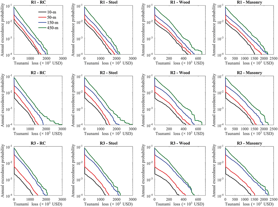
Figure 13. Tsunami loss curves at three locations in Onagawa.

FIGURE 14

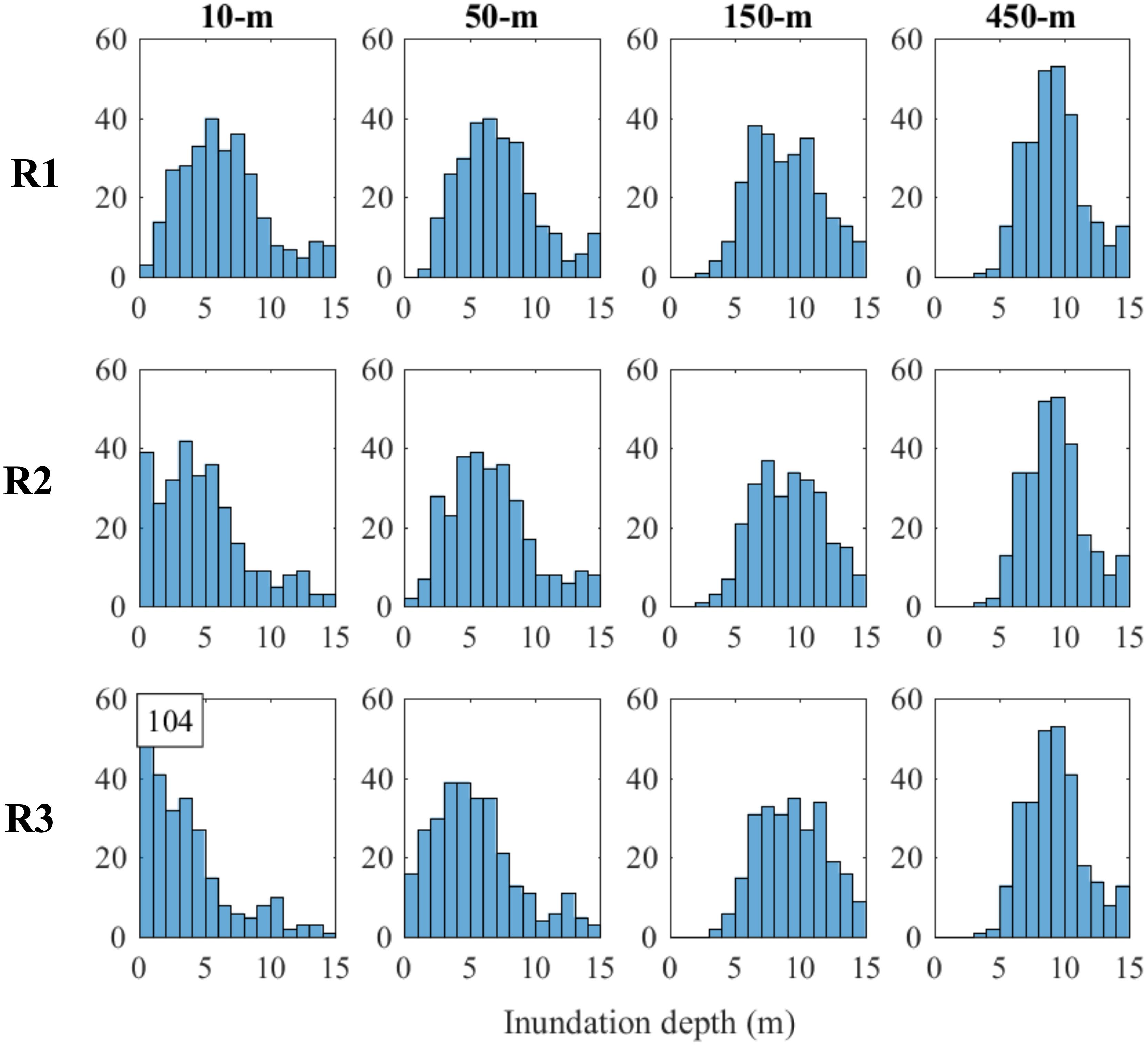
Figure 14. Inundation depth distribution at three locations in Onagawa for the M_w 9.0 events by considering different DEM resolutions (The counts exceeding the y axis limit are indicated in a box). The histogram in each subfigure panel is based on 300 stochastic slip models.

To summarize, tsunami risk is very sensitive to DEM resolution because of the topographic features of Onagawa. For tsunami risk at specific locations, the realistic representation of elevation is vitally important. The 50-m DEM, which is the finest DEM apart from the 10-m one, still cannot ensure the accurate representation of elevation and can cause significant differences in estimated local tsunami loss.

Tsunami Insurance Rate Differentiation

The current earthquake insurance policy does not differentiate properties having different tsunami risks. Given the sensitivity of tsunami risk to building location as demonstrated in the preceding sections, the premium rate differentiation for tsunami insurance is considered based location attributes (i.e., coastal topography, distance to the coast, and elevation). Sendai is focused on to consider the influence of distance from the coast because Sendai is on a plain coast, while Onagawa is considered to examine the influence of elevation because the buildings in Onagawa are located particularly close to the coastline with rapidly rising elevation. More specifically, different locations in Sendai and Onagawa (i.e., P1 to P4 in Sendai and R1 to R3 in Onagawa) are considered to investigate the local tsunami risks on pure premiums for four types of structures (i.e., RC, steel, masonry, and wood). As found in this study that local tsunami risk is sensitive to DEM resolution, to differentiate tsunami insurance premium rates for buildings having different location attributes, tsunami simulations are performed using the 10-m DEM.

The pure premium rates are calculated based on EP curves for each case (in terms of location and structural type) after applying insurance policy parameters (see Eq. (16)). The calculated rates at individual locations are summarized in Table 2. The insurance rates at P1-P4 are differentiated by distance from the coast, while those at R1-R3 are differentiated by land elevation. The rates distinguishing structural types indicate that wood structures have the highest rates and RC structures have the lowest rates, and steel and masonry structure have similar rates. In Sendai with plain coast, the insurance rate at P1 is significantly greater than other locations, regardless of structural type. The rate drops significantly from P1 to P2, and mildly decreases from P2 to P3. Then the rate is almost halved from P3 to P4, with the distance increasing from 1.5 km to 2.0 km. For wood structures, which is the main building material for residential houses in Japan, the rates at P2 and P3 are about 11% of the rates at P1, and the rates at P4 are only 4% of the rates at P1. In Onagawa with ria coast, a significant decrease of rates is seen from R1 to R2 and R3, mainly due to the rise of land elevation. The rates at R1 are almost twice as large as the rates at R2 and the rates at R3 are reduced to about 28% of the rates at R1. Table 3 shows tsunami insurance pure premium rates for wood structures based on DEMs of different resolutions. DEM of lower resolution is less capable of reflecting the variability of local tsunami risk due to different distances from the coastline and different elevations, and result in more uniform insurance rates at different locations.

TABLE 2

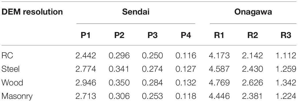
Table 2. Tsunami insurance pure premium rates at different locations (per 1000 insured value).

TABLE 3

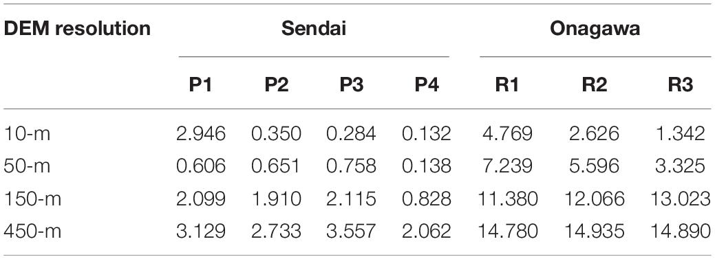
Table 3. Tsunami insurance pure premium rates for wood structures using DEMs of different resolutions (per 1000 insured value).

In Sendai, the coarser DEMs tend to overestimate the rates at farther locations (i.e., P2, P3, and P4). When the grid resolution is 450 m, the rates for the four locations are almost uniform, while the rates at P2, P3, and P4 are reduced to only 11%, 9%, and 4% of the rate at P1 when the finer 10-m resolution is considered. For the 10-m DEM, about 90% drop of the rate is seen from P1 to P2, while the rates at P1 and P2 are similar for the other three DEMs. Although the 50-m DEM, which is the second finest DEM, gives similar tsunami loss results as the 10-m DEM for the whole Sendai, it still cannot reflect the variability in local tsunami risk. The rate at P1 is only about one-fifth of that for the 10-m resolution case, while the rates at P2 and P3 are about twice the rates for the 10-m resolution case. The cases of 450-m resolution is the most unreliable as there is a large discrepancy in rates, and the rates at P2, P3, and P4 are dramatically higher by a factor of 7, 12, and 16 times, respectively, than those given by the 10-m DEM. Therefore, the resolution of DEM has a tremendous impact on the accuracy of tsunami insurance rate-making and the inaccurate elevation can lead to significant errors in the insurance rates, especially at local scales.

In Onagawa, the DEM of low resolution is more likely to cause substantial errors in elevation assigned to locations close to one another. The assigned elevations based on a coarse DEM can be significantly different from what it is, resulting in an inaccurate estimation of local tsunami risk (Table 1). Consequently, the errors caused by using inaccurate elevation models result in unreliable local tsunami insurance rates, as can be found in Table 3. Compared to the rates using the 10-m DEM, the rates given by the other three coarser DEMs are higher at all three locations. A coarser DEM results in higher rates for the Onagawa case. Taking R1 as an example, the rates given by the 50-m, 150-m, and 450-m DEMs are 1.5, 2.4, and 3.1 times greater than the rate given by the 10-m DEM. In addition to the higher rates caused by the coarser DEMs, in Onagawa a coarser DEM also tends to overestimate the rate for a location with lower elevation while overestimate the rate for a location with higher elevation. For the 10-m resolution case, the insurance rate drops by 45% and 72% from R1 to R2 and R1 to R3, respectively, while the rates become almost the same when the grid size is increased to 150 m or 450 m. Even for the second finest DEM of 50 m, the rate at R3 is only 55% lower than the rate at R1, while this difference based on the 10-m DEM is more than 70%. It is emphasized that the disparity in pure premium rate at single locations does not necessarily happen in the total regional tsunami loss, because a building portfolio includes buildings at various locations; however, gross under- or overestimation of premium rates is possible as shown in Figure 13. Therefore, the rate differentiation by elevation is viable only when tsunami risk calculation is able to accurately capture the differences in elevation using a fine DEM.

Conclusion

Based on the stochastic tsunami modeling method, the uncertainty in tsunami risk caused by different DEM resolutions was investigated. To consider different coastal topography, Sendai (coastal plain) and Onagawa (ria coast) were focused upon. The differences on tsunami loss estimation were evaluated at a regional scale as well as for single locations. From the stochastic tsunami loss estimation results, the following conclusions can be dawn:

• The DEM resolution has a significant influence on tsunami loss estimation, especially for local tsunami risk assessment. The coarser DEM tends to underestimate the tsunami intensity at some places, while overestimating it at some other places. Therefore, the accuracy of resulted tsunami loss depends on the location of buildings as well.

• When there is more variation in land elevation at a regional scale, a greater difference is caused by using a coarser DEM. For a plain terrain of Sendai, the 50-m DEM can still produce a loss estimation similar to that of the 10-m DEM, but the 150-m and 450-m DEMs tend to overestimate the total tsunami loss dramatically. Using a coarser DEM tends to underestimate the tsunami loss for the most risky areas but tends to overestimate it for the least risky areas. The 150-m and 450-m DEMs are not able to give a reasonable tsunami loss estimation for both Sendai and Onagawa.

• The tsunami risk at single locations is more sensitive to DEM resolution than regional tsunami losses. For local tsunami risk, DEM resolution controls the accuracy of assigned elevations, which determines the accuracy of local tsunami loss estimation. Even for Sendai, the 50-m resolution is likely to result in significant bias in estimated tsunami losses for single locations with respect to those based on the 10-m DEM. In Onagawa, only 10-m DEM is capable of producing accurate tsunami loss estimation at single locations.

The findings of the influence of DEM resolution have major implications for tsunami insurance rate differentiation by considering the location attributes. The main conclusions from the case study are summarized as follows:

• Because of the localized nature of tsunami risks, elevation data of low resolution like 150 m and 450 m are not capable of simulating the realistic inundation scales. For both regional and local tsunami risk assessments, 150-m and 450-m DEMs are not recommended for use, which can cause substantial errors. For regional tsunami loss, 50-m DEM is acceptable, which gives less than 20% differences in comparison to the 10-m resolution for the case study sites.

• The location of buildings makes a significant difference to local tsunami risk, which is related to the distance from the coast and elevation. For the fair pricing of tsunami insurance, the distance from the coast and land elevation should be taken into account. The increase of distance from the coastline and increase of elevation significantly reduce the tsunami insurance premium. A coarser DEM is less able to distinguish the geographical differences and tends to generate more uniform (and probably biased) premium rates for different locations.

Data Availability

All datasets generated for this study are included in the manuscript and/or the supplementary files.

Author Contributions

All authors listed have made a substantial, direct and intellectual contribution to the work, and approved it for publication.

Funding

The research was supported by the Canada Research Chair in Multi-Hazard Risk Assessment program at Western University (950-232015) and the NSERC Discovery Grant (RGPIN-2019-05898).

Conflict of Interest Statement

The authors declare that the research was conducted in the absence of any commercial or financial relationships that could be construed as a potential conflict of interest.

The handling Editor is currently organizing a Research Topic with one of the authors KG and confirms the absence of any other collaboration.

Footnotes

1. ^ http://www.globalcmt.org/CMTsearch.html
2. ^ http://seisan.ird.nc/USGS/mirror/neic.usgs.gov/neis/epic/code_catalog.html
3. ^ https://www.giroj.or.jp/ratemaking/earthquake/

References

Anagnos, T., and Kiremidjian, A. S. (1988). A review of earthquake occurrence models for seismic hazard analysis. Probab. Eng. Mech. 3, 3–11. doi: 10.1016/0266-8920(88)90002-90001

CrossRef Full Text | Google Scholar

Box, G. E. P., and Cox, D. R. (1964). An analysis of transformations. J. R. Stat. Soc. Ser. B. 26, 211–252.

Google Scholar

Cramer, C. H., Petersen, M. D., Cao, T., Toppozada, T. R., and Reichle, M. (2000). A time-dependent probabilistic seismic-hazard model for California. Bull. Seismol. Soc. Am. 90, 1–21. doi: 10.1785/0119980087

CrossRef Full Text | Google Scholar

De Risi, R., Goda, K., Yasuda, T., and Mori, N. (2017). Is flow velocity important in tsunami empirical fragility modeling? Earth Sci. Rev. 166, 64–82. doi: 10.1016/j.earscirev.2016.12.015

CrossRef Full Text | Google Scholar

Ellsworth, W. L., Matthews, M., and Nadeau, R. (1999). A Physically based Earthquake Recurrence Model for Estimation of Long-Term Earthquake Probabilities. Reston, VA: U.S. Geological Survey.

Google Scholar

Fewtrell, T. J., Bates, P. D., Horritt, M., and Hunter, N. M. (2008). Evaluating the effect of scale in flood inundation modelling in urban environments. Hydrol. Process. 22, 5107–5118. doi: 10.1002/hyp.7148

CrossRef Full Text | Google Scholar

Fitzenz, D. D., and Nyst, M. (2015). Building time-dependent earthquake recurrence models for probabilistic risk computations. Bull. Seismol. Soc. Am 105, 120–133. doi: 10.1785/0120140055

CrossRef Full Text | Google Scholar

Fujii, Y., and Satake, K. (2007). Tsunami source of the 2004 sumatra-andaman earthquake inferred from tide gauge and satellite data. Bull. Seismol. Soc. Am. 97, S192–S207. doi: 10.1785/0120050613

CrossRef Full Text | Google Scholar

Geist, E. L., and Parsons, T. (2011). Assessing historical rate changes in global tsunami occurrence. Geophys. J. Int. 187, 497–509. doi: 10.1111/j.1365-246X.2011.05160.x

CrossRef Full Text | Google Scholar

Goda, K. (2019). Time-dependent probabilistic tsunami hazard analysis using stochastic source models. Stoch. Environ. Res. Risk Assess. 33, 341–358. doi: 10.1007/s00477-018-1634-x

CrossRef Full Text | Google Scholar

Goda, K., and De Risi, R. (2017). Probabilistic tsunami loss estimation methodology: stochastic earthquake scenario approach. Earthq. Spectra 33, 1301–1323. doi: 10.1193/012617eqs019m

CrossRef Full Text | Google Scholar

Goda, K., Mai, P. M., Yasuda, T., and Mori, N. (2014). Sensitivity of tsunami wave profiles and inundation simulations to earthquake slip and fault geometry for the 2011 Tohoku earthquake. Earth Planet. Space 66, 1–20.

Google Scholar

Goda, K., Yasuda, T., Mori, N., and Maruyama, T. (2016). New scaling relationships of earthquake source parameters for stochastic tsunami simulations. Coast. Eng. J. 58, 1–40. doi: 10.1142/S0578563416500108

CrossRef Full Text | Google Scholar

Gomberg, J., Belardinelli, M. E., Cocco, M., and Reasenberg, P. (2005). Time-dependent earthquake probabilities. J. Geophys. Res. 110, 1–12. doi: 10.1029/2004JB003405

CrossRef Full Text | Google Scholar

Goto, C., Ogawa, Y., and Shuto, N. (1997). Numerical Method of Tsunami Simulation With the Leap-Frog Scheme. Paris: UNESCO.

Google Scholar

Gray, R. J., and Pitts, S. M. (2012). Risk Modelling in General Insurance: From principles to Practice. Cambridge: Cambridge University Press.

Google Scholar

Grezio, A., Babeyko, A., Baptista, M. A., Behrens, J., Costa, A., Davies, G., et al. (2017). Probabilistic tsunami hazard analysis: multiple sources and global applications. Rev. Geophys. 55, 1158–1198. doi: 10.1002/2017RG000579

CrossRef Full Text | Google Scholar

Griffin, J., Latief, H., Kongko, W., Harig, S., Horspool, N., Hanung, R., et al. (2015). An evaluation of onshore digital elevation models for modeling tsunami inundation zones. Front. Earth Sci. 3:32. doi: 10.3389/feart.2015.00032

CrossRef Full Text | Google Scholar

Gutenberg, B., and Richter, C. F. (1956). Magnitude and energy of earthquakes. Ann. Geophys. 9, 1–15. doi: 10.4401/ag-5590

CrossRef Full Text | Google Scholar

Headquarters for Earthquake Research Promotion [HERP], (2013). Investigations of Future Seismic Hazard Assessment. Tokyo: Japanese Govern.

Google Scholar

Ioualalen, M., Asavanant, J., Kaewbanjak, N., Grilli, S. T., Kirby, J. T., and Watts, P. (2007). Modeling the 26 december 2004 indian ocean tsunami: case study of impact in thailand. J. Geophys. Res. 112, 1–21.

Google Scholar

Kaczmarska, J., Jewson, S., and Bellone, E. (2018). Quantifying the sources of simulation uncertainty in natural catastrophe models. Stoch. Environ. Res. Risk Assess. 32, 591–605. doi: 10.1007/s00477-017-1393-1390

CrossRef Full Text | Google Scholar

Kagan, Y. Y., and Jackson, D. D. (2013). Tohoku earthquake: a surprise? Bull. Seismol. Soc. Am. 103, 1181–1194. doi: 10.1785/0120120110

CrossRef Full Text | Google Scholar

Kaiser, G., Scheele, L., Kortenhaus, A., Løvholt, F., Römer, H., and Leschka, S. (2011). The influence of land cover roughness on the results of high resolution tsunami inundation modeling. Nat. Hazards Earth Syst. Sci. 11, 2521–2540. doi: 10.5194/nhess-11-2521-2011

CrossRef Full Text | Google Scholar

Kajitani, Y., Chang, S. E., and Tatano, H. (2013). Economic Impacts of the 2011 tohoku-oki earthquake and tsunami. Earthq. Spectra 29, S457–S478. doi: 10.1193/1.4000108

CrossRef Full Text | Google Scholar

Kanamori, H. (1972). Mechanism of tsunami earthquakes. Phys. Earth Planet. Interiors 6, 346–359. doi: 10.1016/0031-9201(72)90058-90051

CrossRef Full Text | Google Scholar

Kazama, M., and Noda, T. (2012). Damage statistics (Summary of the 2011 off the Pacific coast of Tohoku earthquake damage). Soils Found. 52, 780–792. doi: 10.1016/j.sandf.2012.11.003

CrossRef Full Text | Google Scholar

Kuzak, D., and Larsen, T. (2005). “Use of catastrophe models in insurance rate making,” in Catastrophe Modeling: A New Approach To Managing Risk, eds P. Grossi, and H. Kunreuther, (New York, NY: Springer), doi: 10.1007/0-387-23129-3-5

CrossRef Full Text | Google Scholar

Lavallée, D., Liu, P., and Archuleta, R. J. (2006). Stochastic model of heterogeneity in earthquake slip spatial distributions. Geophys. J. Int. 165, 622–640. doi: 10.1111/j.1365-246x.2006.02943.x

CrossRef Full Text | Google Scholar

Mai, P. M., and Beroza, G. C. (2002). A spatial random field model to characterize complexity in earthquake slip. J. Geophys. Res. 107, ESE10-1–ESE10-21.

Google Scholar

Mori, N., Takahashi, T. and The Tohoku Earthquake Tsunami Joint Survey Group, (2012). Nationwide post event survey and analysis of the 2011 tohoku earthquake tsunami. Coast. Eng. J. 54:1250001. doi: 10.1142/s0578563412500015

CrossRef Full Text | Google Scholar

Muhammad, A., and Goda, K. (2018). Impact of earthquake source complexity and land elevation data resolution on tsunami hazard assessment and fatality estimation. Comput. Geosci. 112, 83–100. doi: 10.1016/j.cageo.2017.12.009

CrossRef Full Text | Google Scholar

Okada, Y. (1985). Surface deformation due to shear and tensile faults in a half-space. Bull. Seismol. Soc. Americaoc. Am. 75, 1135–1154.

Google Scholar

Pardo-Igúzquiza, E., and Chica-Olmo, M. (1993). The Fourier integral method: an efficient spectral method for simulation of random fields. Math. Geol. 25:177. doi: 10.1007/bf00893272

CrossRef Full Text | Google Scholar

Sangati, M., and Borga, M. (2009). Influence of rainfall spatial resolution on flash flood modelling. Nat. Hazards Earth Syst. Sci. 9, 575–584. doi: 10.5194/nhess-9-575-2009

CrossRef Full Text | Google Scholar

Satake, K. (1995). Linear and nonlinear computations of the 1992 Nicaragua earthquake tsunami. Pure Appl. Geophys. 144, 455–470. doi: 10.1007/BF00874378

CrossRef Full Text | Google Scholar

Satake, K., Fujii, Y., Harada, T., and Namegaya, Y. (2013). Time and space distribution of coseismic slip of the 2011 Tohoku earthquake as inferred from tsunami waveform data. Bull. Seismol. Soc. Am. 103, 1473–1492. doi: 10.1785/0120120122

CrossRef Full Text | Google Scholar

Schäfer, A. M., and Wenzel, F. (2017). TsuPy: computational robustness in tsunami hazard modelling. Comput. Geosci. 102, 148–157. doi: 10.1016/j.cageo.2017.02.016

CrossRef Full Text | Google Scholar

Suppasri, A., Koshimura, S., Imai, K., Mas, E., Gokon, H., Muhari, A., et al. (2012). Damage characteristic and field survey of the 2011 great east japan tsunami in miyagi prefecture. Coast. Eng. J. 54:1250005. doi: 10.1142/s0578563412500052

CrossRef Full Text | Google Scholar

Synolakis, C., Liu, P., Carrier, G., and Yeh, H. (1997). Tsunamigenic sea-floor deformations. Science 278, 598–600. doi: 10.1126/science.278.5338.598

CrossRef Full Text | Google Scholar

Tang, L., Titov, V. V., and Chamberlin, C. D. (2009). Development, testing, and applications of site-specific tsunami inundation models for real-time forecasting. J. Geophys. Res. 114, 1–22. doi: 10.1029/2009JC005476

CrossRef Full Text | Google Scholar

Tanioka, Y., and Satake, K. (1996). Tsunami generation by horizontal displacement of ocean bottom. Geophys. Res. Lett. 23, 861–864. doi: 10.1029/96gl00736

CrossRef Full Text | Google Scholar

Titov, V., Rabinovich, A. B., Mofjeld, H. O., Thomson, R. E., and Gonzalez, F. I. (2005). The global reach of the 26 december 2004 Sumatra tsunami. Science 309, 2045–2048. doi: 10.1126/science.1114576

PubMed Abstract | CrossRef Full Text | Google Scholar