Feasibility to Use Continuous Magnetotelluric Observations for Monitoring Hydrothermal Activity. Numerical Modeling Applied to Campi Flegrei Volcanic System (Southern Italy)

Introduction

Monitoring a hydrothermal system involves the recognition of time variations in chemical, physical, and thermal parameters of the fluids circulating through pores and fractures of the host rocks. Linking the variations of such parameters to changes in the physical state of the system is crucial for understanding behavior and evolution of a hydrothermal system for both volcanic hazard assessment and geothermal energy exploitation.

In the last few decades, several monitoring techniques based on geochemical and/or geophysical methods have been proposed and successfully applied (e.g., Berrino et al., 1984; Lowenstern et al., 2006; Hurwitz et al., 2007; Chiodini et al., 2010; Biggs et al., 2014; Portier et al., 2018). Among these, the most commonly used involve geochemical analyses of the fluids emitted from the surface and ground deformation studies. In particular, chemical and isotopic analyses of hydrothermal fluids are widely used to infer depth and origin (magmatic or crustal) of the fluid source and, in case of volcanic hydrothermal systems, possible upwelling of the magma source (e.g., Bibby et al., 1995; Chiodini et al., 1998; Moran et al., 2000; Cardellini et al., 2003a, b; Finizola et al., 2003; Lowenstern et al., 2006; Rouwet et al., 2009). Whereas, ground deformation measurements are commonly used to obtain information on inflation or deflation of the hydrothermal system, possibly due to variations in its pressure and fluid content, and to infer the probability of explosion/eruption (e.g., Bartel et al., 2003; Puskas et al., 2007; Chiodini et al., 2010). Although these techniques are very effective in monitoring hydrothermal systems, they have some limitations. Specifically, the geochemical monitoring is linked to the occurrence of hydrothermal surface manifestations (e.g., springs, geysers, and fumaroles) and to the feasibility of fluid sampling, which can be severely limited in not easily accessible areas. While the main limit of the ground deformation monitoring lies in the data inversion problem (i.e., in retrieving the deformation causative source) that is poorly constrained as the measurements are limited to the ground surface. Therefore, in the last few decades these methods have been suitably integrated with other kind of techniques to assess the behavior of hydrothermal (or geothermal) systems. In particular, electric and electromagnetic geophysical methods have been proposed as useful tools for studying the physical processes governing their dynamics (e.g., Di Maio et al., 1998; Zlotnicki et al., 1998; Di Maio et al., 2000; Sasai et al., 2001; Zlotnicki et al., 2006; Utada et al., 2007; Legaz et al., 2009; Byrdina et al., 2014; Di Maio and Berrino, 2016; Gresse et al., 2017; Wawrzyniak et al., 2017; Ladanivskyy et al., 2018). The underlying idea is that, since the Earth subsurface resistivity distribution is sensitive to presence, composition, and temperature of the fluids along permeable fracture systems (Hersir and Björnsson, 1991; Ussher et al., 2000; Hersir and Árnason, 2009), observing resistivity changes over time may give useful insights on possible variations in the physical properties of the system. It is reasonable, indeed, to assume that resistivity varies substantially as result of changes in fluid composition, flow pattern, heat source, and water pH. It is worth noting that the observed resistivity variations can also reflect stress-induced structural changes.

Among all the geophysical methods that investigates the underground resistivity distribution, the magnetotelluric (MT) method presents two features that make it appropriate for monitoring purposes: (i) it investigates a wide range of depths, from hundreds of meters to hundreds of kilometers, allowing to retrieve information on the system at different scales; and (ii) it is a passive geophysical method, so it does not require an artificial energy source reducing the costs of a continuous monitoring. Although MT is widely used to characterize hydrothermal and geothermal systems (e.g., Stanley et al., 1977; Volpi et al., 2003; Heise et al., 2008; Newman et al., 2008; Munoz, 2014; Didana et al., 2015; Amatyakul et al., 2016; Peacock et al., 2016; Samrock et al., 2018), using MT as monitoring tool is still a new field of research, likely due to its sensitivity to anthropogenic noises. However, the advancements reached over the last few decades in the MT data processing make the method reliable also in presence of high level of cultural noise (e.g., Bahr, 1988; Egbert, 1997; Caldwell et al., 2004; Chave and Thomson, 2004; Weckmann et al., 2005; Larnier et al., 2016; Carbonari et al., 2018; Platz and Weckmann, 2019). To our knowledge, continuous MT measurements over a long period of time were carried out only by Aizawa et al. (2011), who monitored temporal changes in electrical resistivity at Sakurajima volcano for 180 days. They found variations in apparent resistivity of approximately ±20% suggesting possible degassed volatile migration laterally through a fracture network, as well as vertically through the volcano conduit. On the other hand, several MT surveys designed to monitor fluid stimulations for Enhanced Geothermal Systems (EGS) (Bedrosian et al., 2004; Geiermann and Schill, 2010; Peacock et al., 2012, 2013; MacFarlane et al., 2014; Didana et al., 2017) have been performed to assess the effectiveness of continuous MT observations in revealing lateral migration of fluids. For example, Peacock et al. (2012) observed an average decrease of 10 and 5% in the xy and yx components of the apparent resistivity, respectively, through MT measurements repeated in a time interval of 4 days after a fluid stimulation down to a depth of 3.6 km at Paralana borehole (Australia). Moreover, further analyses (Peacock et al., 2013) showed that the injected fluids mostly propagated in the N-NE direction, which corresponds to the pre-existing fault system orientation. Similar results have been also found by Didana et al. (2017) at Cooper Basin EGS (South Australia).

Conversely from the quoted studies, in the present work we propose to study the sensitivity of MT monitoring in detecting hydrothermal system variations by modeling possible evolution scenarios of the system dynamics and by estimating at selected time steps the synthetic response of MT soundings located along a profile crossing the hydrothermal system. The proposed approach is applied to the hydrothermal system of the Campi Flegrei (CF) volcanic district (Southern Italy), for which long geochemical and ground deformation data series, acquired since the early eighties (Chiodini et al., 2003; Todesco et al., 2004; Caliro et al., 2007), have allowed to define an accurate 3D petrophysical model (Petrillo et al., 2013).

Materials and Methods

The Magnetotelluric Method

Magnetotellurics is a passive geophysical method aimed at defining subsurface electrical resistivity distribution of the study area (e.g., Wait, 1962; Vozoff, 1990). MT is based on the simultaneous measurements on the Earth’s surface of electric and magnetic horizontal components of the natural electromagnetic field (i.e., the magnetotelluric field), which are linearly related in the frequency domain through the transfer function defined as the impedance tensor. The latter plays an important role in the MT prospecting as it contains information on subsurface resistivity structure. In the frequency domain, the relationship that links the electric and magnetic fields reads as follows:

$$\left(\begin{array}{c}\hfill E_x\hfill \\ \hfill E_y\hfill \end{array}\right)=\left(\begin{array}{cc}\hfill Z_{xx}\mathit{\hspace{1em}}\hfill & \hfill Z_{xy}\hfill \\ \hfill Z_{yx}\mathit{\hspace{1em}}\hfill & \hfill Z_{yy}\hfill \end{array}\right)\cdot \left(\begin{array}{c}\hfill H_x\hfill \\ \hfill H_y\hfill \end{array}\right),(1)$$

where E_x, E_y and H_x, H_y are, respectively, the Fourier transforms of the horizontal electric and magnetic components of the MT field and Z_ij (where i,j = x,y) are elements of the impedance tensor Z. According to the diffusive nature of the MT field, electromagnetic waves of different frequencies reach different depths. In particular, the smaller the frequency, the deeper the penetration power (Vozoff, 1990). Thus, the impedance tensor evaluation at different frequencies will provide estimates of the electrical resistivity at different depths. In case of a homogeneous Earth, the impedance tensor is an anti-diagonal matrix and is related to the electrical resistivity by the following equation:

$${\mathrm{\rho }}_{xy}={\mathrm{\rho }}_{yx}=\frac{1}{\mathrm{\omega }\mathrm{\mu }}{\left|Z_{xy}\right|}^2=\frac{1}{\mathrm{\omega }\mathrm{\mu }}{\left|Z_{yx}\right|}^2,(2)$$

where ρ is the electrical resistivity, ω is the angular frequency, and μ is the magnetic permeability of the subsurface volume involved by the electromagnetic induction. In case of an inhomogeneous subsoil, whose structure can be reasonably described with a 1D or 2D electrical dimensionality, which is a good approximation for several geological contexts (e.g., major fault zones, subduction areas, and axisymmetric volcanic edifices), the impedance tensor is still an anti-diagonal matrix (Bahr, 1988), but the resistivity given by Eq. 2 becomes an apparent resistivity value, i.e., a volume average of the real resistivity values that characterize the underground structures affected by the electromagnetic induction. Thus, Eq. 2 becomes:

$${\mathrm{\rho }}_{axy}=\frac{1}{\mathrm{\omega }\mathrm{\mu }}{\left|Z_{xy}\right|}^2\ne {\mathrm{\rho }}_{ayx}=\frac{1}{\mathrm{\omega }\mathrm{\mu }}{\left|Z_{yx}\right|}^2,(3)$$

where ρ_axy and ρ_ayx are the apparent resistivity values calculated for each frequency ω. These values, displayed as function of frequency (or period), allow to obtain qualitative information on both depth resistivity variations and subsurface electrical dimensionality.

It is worth noting that, for 2D earth resistivity structures, the electric component parallel to a lateral resistivity discontinuity (e.g., fault, dyke) induces a magnetic field perpendicular to the discontinuity and vice versa. This allows the decoupling of the MT field into two independent modes: the transverse electric mode (TE mode), which describes electric currents flowing parallel to the discontinuity, and the transverse magnetic mode (TM mode), which describes electric currents flowing perpendicular to the discontinuity direction. Thus, the TM mode is more sensitive to lateral resistivity variations (Simpson and Bahr, 2005).

Sensitivity of MT Monitoring to Hydrothermal System Variations

The MT monitoring sensitivity study presented here aims to quantify how much and how fast the magnetotelluric response varies after a change in the initial state of a hydrothermal system. The entire procedure is summarized in the flow chart shown in Figure 1. The first two steps of the procedure concern the building of a 3D realistic petrophysical model of the hydrothermal system under investigation, and the definition of possible variations of its initial conditions according to the characteristics of the system source and the properties of the host rocks. The third step involves the simulation of the hydrothermal system time evolution related to a fixed change of its initial conditions. The fourth step founds on the transformation of the petrophysical parameters, provided by the numerical simulation at selected time steps, to the corresponding electrical resistivity values by using a suitable analytical relationship. The latter allows to transform, for each time step, the 3D petrophysical model into a 3D resistivity model, which in turn permits to calculate the 2D synthetic MT response (fifth step in Figure 1) at different sounding stations located along a surface profile overlying the hydrothermal system. Finally, the MT monitoring sensitivity is analyzed in terms of time required for observing significant apparent resistivity variations. In the present study, the proposed procedure has been applied to the hydrothermal system of CF, by considering a synthetic continuous 2D MT survey performed along a profile centered on the CF caldera.

FIGURE 1

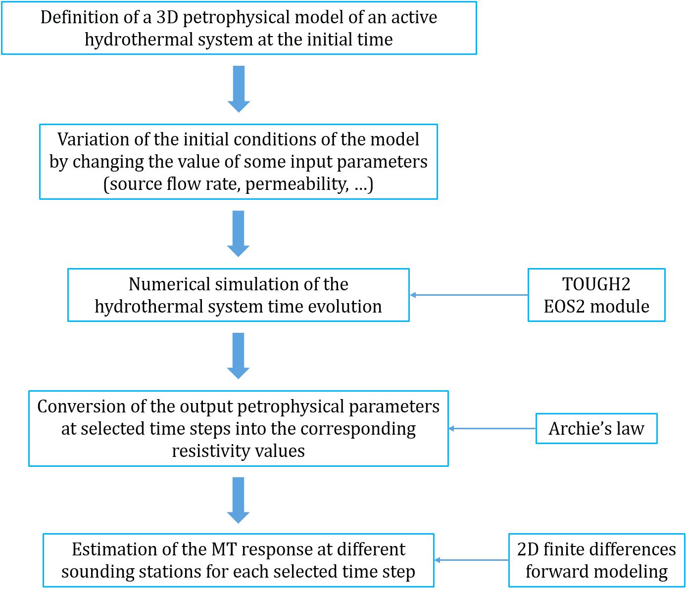
Figure 1. Flow chart of the procedure proposed to study the MT sensitivity to hydrothermal system variations.

The Campi Flegrei Model

The CF area (Figure 2) is an active volcanic district located close to the city of Naples (Southern Italy) that has given rise to almost 70 eruptions in the last 15 kyr (Isaia et al., 2009), the last one occurred in 1538 AD (Di Vito et al., 1987; Rosi and Sbrana, 1987). The CF caldera hosts a hydrothermal system that is well developed mainly at the center of the volcanic district, in the area of the Solfatara crater (red dot in Figure 2). The main surface-manifestations of volcanic activity are represented by ground deformation and geothermal and hydrothermal activity (e.g., intense fumarolic flows, diffuse gas emissions, and anomalous temperature gradient). The latter likely responsible for the significant periodic variations in the ground surface (bradyseism phenomena) observed in the CF area (Tedesco et al., 1988; Di Vito et al., 1999; Chiodini et al., 2003; Todesco et al., 2004; De Natale et al., 2006; Lima et al., 2009).

FIGURE 2

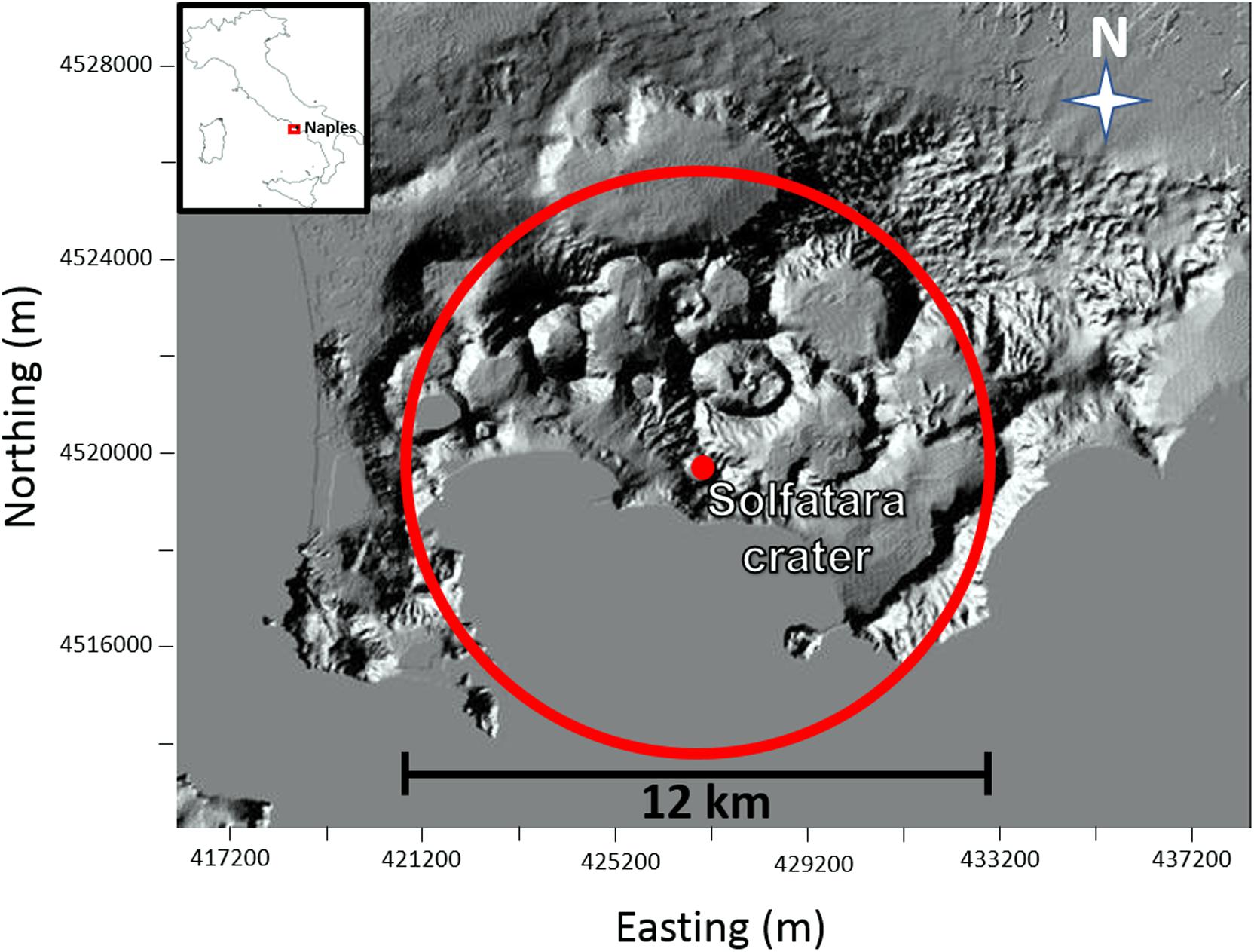
Figure 2. Campi Flegrei volcanic area (Southern Italy). The red circle shows the diameter of the petrophysical model used to simulate the dynamics of the CF hydrothermal system. The red point indicates the center of the model that is located at the Solfatara volcano.

In the last few decades, several models have been proposed to explain the CF hydrothermal system dynamics. Currently, most authors (Chiodini et al., 2003, 2012, 2016; Todesco et al., 2003, 2004; Caliro et al., 2007; Petrillo et al., 2013; Afanasyev et al., 2015) agree with a conceptual model consisting of a vertical plume, about 2.5 km deep, fed by both deep magmatic gas accumulation and vaporization of liquids of meteoric origin. In particular, the CF model employed for the numerical simulations presented in this work is that proposed by Petrillo et al. (2013). It has a cylindrical shape, with diameter of 12 km and height of 3 km, centered on the Solfatara Crater and is composed of 11,800 cells with volumes ranging from 1.95 × 10⁶ to 9.32 × 10⁷ m³, with a finer discretization near the upper boundary and along the central part of the system describing the fluid upwelling zone (Figure 3). The model hypothesizes the presence of a source of fluids (H₂O and CO₂) in a cell of volume 1.53 × 10⁷ m³ located along the cylinder axis and centered at a depth of 2.6 km (red rectangle in Figure 3) that emits 17 kg/s of CO₂ and 50 kg/s of H₂O with an enthalpy of 3.3 × 10⁵ and 2.7 × 10⁶ J/kg, respectively. Such rates of emission have been chosen in agreement with the measured values of CO₂ and H₂O/CO₂ by Caliro et al. (2007) and Chiodini et al. (2011). The model, developed using the TOUGH2 code (Pruess, 1991), defines properties of the host rocks of the hydrothermal system in terms of temperature, pressure, and gas saturation values, as well as porosity and permeability values. The porosity values have been obtained by deriving a linear relation between density and porosity data measured on outcrop and deep well samples collected in the whole CF area (Petrillo et al., 2013). Then, the porosity data have been used to estimate the permeability values by using the relation proposed by Costa (2006). We note that the CF model we used is considered a realistic approximation of the actual state of the CF volcanic system by many authors (Chiodini et al., 2003, 2012; Todesco et al., 2004; Caliro et al., 2007, 2014; Amoruso et al., 2014), as it is able to reproduce the surface geochemical and temperature data collected in the area. In particular, Figure 4 shows the temperature and gas saturation distributions obtained for the cross section along the W-E profile indicated by the red line in Figure 3. As it can be seen, the model exhibits a plume of high temperature and gas saturation just above the source of fluids. It is worth noting that, while the temperature of the plume decreases toward the surface, its gas saturation shows a more complex pattern. Indeed, two zones of complete gas saturation are observed: a deeper zone, which is located in proximity of the system source and extends from 1000 to 2600 m b.g.l., and a shallower zone, which extends from approximately 50 to 250 m b.g.l. The latter is possibly ascribed to the combined effect of temperature and pressure that, due to the high temperatures at shallow depths (T ≥ 150°C and z ≤ 200 m), allows the boiling of a larger amount of water.

FIGURE 3

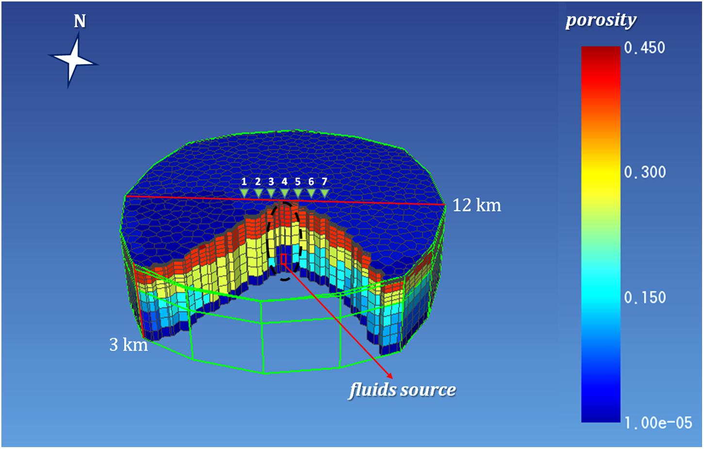
Figure 3. Campi Flegrei model shown in terms of porosity distribution. The red line indicates the profile along which the synthetic MT response at the stations 1–7 has been calculated. The black dashed ellipse indicates the portion of the hydrothermal system whose permeability values have been changed to simulate the effect of a permeability increase on the system dynamics (see section “Scenario II: Effect of Permeability Increasing”).

FIGURE 4

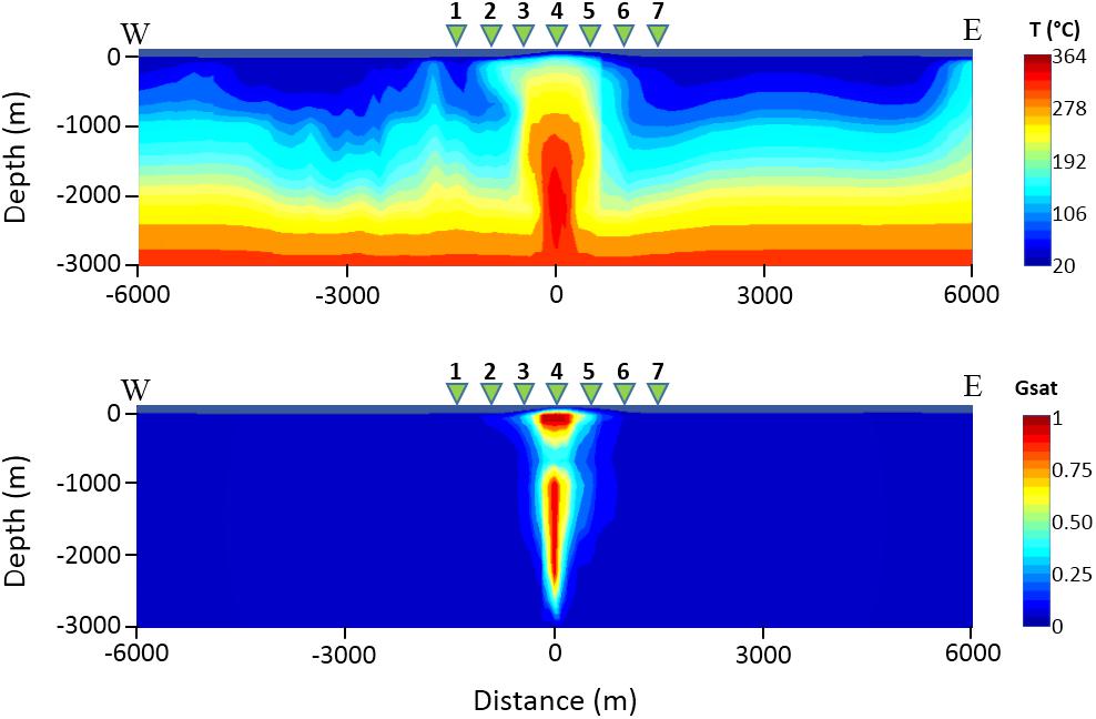
Figure 4. Temperature (upper panel) and gas saturation (lower panel) distributions retrieved from the Campi Flegrei model proposed by Petrillo et al. (2013) along the red line shown in Figure 3. The green triangles 1–7 indicate the MT stations.

Analytical Relationship Between Petrophysical Properties and Electrical Resistivity

Possible relationships linking petrophysical properties to electrical resistivity have been investigated with the aim of transforming the selected petrophysical model of the CF area into an electrical resistivity distribution. The well-known Archie’s law (Archie, 1942; Glover et al., 2000; Glover, 2016) proved to be the most appropriate for our study when modified to take into account the effect of the temperature on the water resistivity (Dakhnov, 1962; Quist and Marshall, 1968; Hersir and Árnason, 2009):

$$\mathrm{\rho }=a{S}^{-n}{\mathrm{\phi }}^{-m}\left[\frac{{\mathrm{\rho }}_{23}}{1+\mathrm{\alpha }(T-23)}\right],(4)$$

where ρ (Ωm) is the resistivity, a is the rock tortuosity factor, S is the water saturation, φ is the rock porosity, α (°C^–1) is the water temperature coefficient, n is the rock saturation exponent, m is the rock cementation exponent, T (°C) is the water temperature, ρ₂₃ is the water resistivity at the temperature of 23°C (Schlumberger, 2009). In this work, we used tortuosity factor and cementation exponent values typical of semi-consolidated tuffs, i.e., 0.5 and 2.8, respectively (Keller and Frischknecht, 1966; Keller, 1967). We note that the modified Archie’s equation (i.e., Eq. 4) has been validated by comparing the resistivity estimates retrieved from the petrophysical model to existing resistivity data on CF area. Interestingly, the chosen relationship allowed us to predict along the central portion of the analyzed profile (red line in Figure 3) the occurrence of: (i) a shallow region (i.e., above 300 m below ground level) characterized by relatively high resistivity values, which well match the results by Gresse et al. (2017), (ii) a highest conductivity zone below 1000 m depth, which is in very good agreement with the resistivity behavior recently found by Siniscalchi et al. (2019) from 2D inversion of audiomagnetotelluric (AMT) data.

Results and Discussion

Sensitivity of MT Monitoring: Results

Starting from the model described in section “The Campi Flegrei Model,” two sets of simulations, which we assume as representative of possible evolutions of active hydrothermal systems, have been performed. The first set involves an increase in the fluid (liquid and/or gas) flow rate emitted from the system source. For volcanic hydrothermal systems like the CF, such an occurrence may be due, for example, to opening of new fractures and/or to magma ascent, which allows the exsolution of a larger amount of gas. The second set of simulations has been performed by increasing the permeability values of rock volume above the system source, which is presumably the zone most affected by the uprising of deep fluids (see black dashed ellipse in Figure 3), keeping fixed the fluid flow rate from the source. This scenario may occur when, for example, an increase in the fluids pressure creates new fractures and/or reopens the pre-existing ones, likely closed by self-sealing processes. The MT monitoring sensitivity has been assessed by assuming the presence of seven magnetotelluric stations, distant 500 m each other, along a profile crossing the center of the CF caldera (red line in Figure 3), whose orientation was chosen based on the outer caldera major axis (Acocella, 2010) and the direction of the main faults in the area, whose strike is predominantly NW−SE. The MT response related to the petrophysical discretized model employed for the numerical simulations has been calculated by using a 2D forward modeling code based on finite differences (Mackie and Madden, 1993; Zhang et al., 1995; Rodi and Mackie, 2001) available in the Geosystem’s WinGLink software package. A 10% error has been assumed for each impedance tensor estimate for taking into account the presence of noise on the MT data. Since no significant variations (i.e., greater than 10% error) have been observed for the MT phases, in the following the MT response will be shown just for the apparent resistivity and, in particular, for the three central MT stations (i.e., 3, 4, and 5 in Figure 3), where the performed numerical simulations found the largest variations in temperature and gas saturation. In this regard, we note that the corresponding variations in the MT signals are found within a 500 m radius from the center of the hypothesized source and this result fits well with the inverted resistivity model retrieved by Siniscalchi et al. (2019) through AMT soundings along a profile crosscutting the Solfatara crater. Finally, we point out that the apparent resistivity curves shown in this work refer to the TM mode, since it is more sensitive than the TE mode to the marked lateral variations observed for both scenarios in the temperature and gas saturation distributions.

Scenario I: Effect of Fluid Flow Rate Increasing

Several simulations have been performed by considering different increases of the fluid flow rate emitted by the system source (see section “The Campi Flegrei Model”). For each increase of the flow rate, which is kept fixed throughout the simulation, the hydrothermal system evolution has been simulated for a time interval of about 3 kyr. During each simulation, the temperature and gas saturation distributions, as well as the MT response at the seven sounding stations, have been estimated at selected time steps along the red line in Figure 3. For all the performed simulations, corresponding to the assumed increases of the fluid flow rate, the hydrothermal system has shown a great inertia, meaning that the analyzed physical parameters, i.e., temperature and gas saturation, have changed very slowly during the simulation time interval. As an example, Figures 5, 6 show the simulation results for a fluid flow rate from the source equal to twice that assumed by Petrillo et al. (2013). Specifically, Figures 5, 6 display the results for a variation of the CO₂ flow rate from 17 to 34 kg/s and a variation of H₂O flow rate from 50 to 100 kg/s. As it can be seen, the temperature (Figure 5) and gas saturation (Figure 6) distributions are mostly constant for the first 30 years, whilst significant variations are observed only after 100 years. The inertia of the system to changes in the fluid flow rate is apparent in Figure 7A, where the ratio between the synthetic apparent resistivity values (ρ_a) and the value of the apparent resistivity at the initial time (ρ_ai), evaluated at period T = 1 s (penetration depth of about 2800–3000 m), has been plotted as a function of time. As it can be seen, the MT response starts to change after a time interval of 30 years for the stations 3 and 5, while it stays unchanged for the central station 4. This finding can be justified by considering a complete saturation in gas of the hydrothermal system under station 4 at the starting time of the simulation process. Conversely, the MT stations 3 and 5, which are symmetrical with respect to the center of the analyzed section, and therefore with respect to station 4 (see Figure 3), show significant variations in the apparent resistivity values estimated after a time interval of 30 years, just when perceptible changes are registered in the gas saturation distribution (see Figure 6). Figure 7B highlights the spatial variation of the apparent resistivity after 100 years of simulation, showing that the region where the MT response is more sensitive to changes in physical parameters covers a space interval of 500 m from the center of the hydrothermal system source. Therefore, the apparent resistivity curves have been calculated at different time steps only for these three central MT stations (Figure 8). As it can be seen, variations in the apparent resistivity are found stronger for periods larger than 0.1 s, corresponding to a penetration depth of about 1400–1500 m, which means that ρ_a starts to increase at deeper depths. The different trend of the MT curves for stations 3 and 5 emphasizes the anisotropy of the system, whose largest effects are observed in the time interval 10–30 years. Indeed, in such an interval the apparent resistivity for periods longer than 1 s first slightly decreases and then increases for the western station 3, while it monotonically increases for the eastern station 5. Moreover, apparent resistivity values at station 5 are found greater than those estimated at station 3. The observed features reflect the asymmetry of the plume, which is slightly wider to the east, below the station 5 (Figure 6). Finally, we note that the monotonic increase of the apparent resistivity curves, observed at the beginning of the simulation at period of about 1 s, moves toward lower periods (about 0.1 s) for larger simulation times. This behavior highlights that the increasing in temperature and gas saturation firstly involves the deeper portion of the hydrothermal system and then reaches its shallowest part (see Figures 5, 6). As mentioned above, similar results have been obtained for different increases in the flow rate. In particular, a reaction time of the system to an increase of the flow fluid rate shorter than 30 years has been observed only for an increase of about four times the original rate.

FIGURE 5

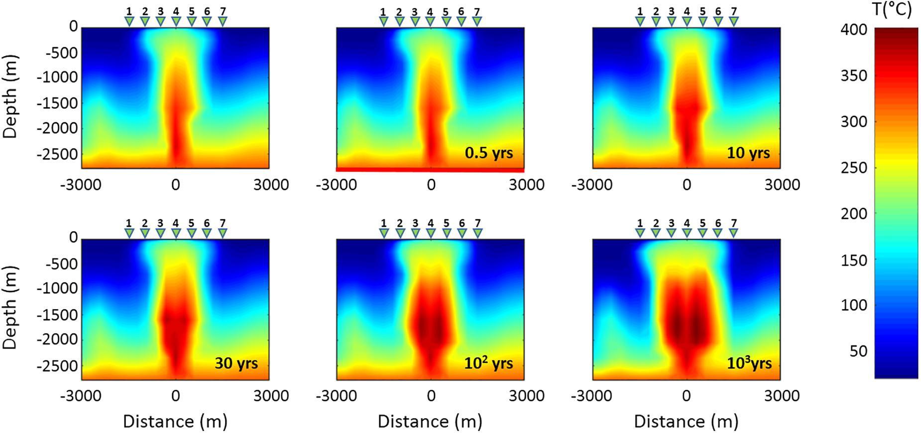
Figure 5. Time evolution of the temperature distribution related to Scenario I in the vertical section along the red line shown in Figure 3. The first panel of the sequence shows the initial temperature distribution. The green triangles 1–7 indicate the MT stations.

FIGURE 6

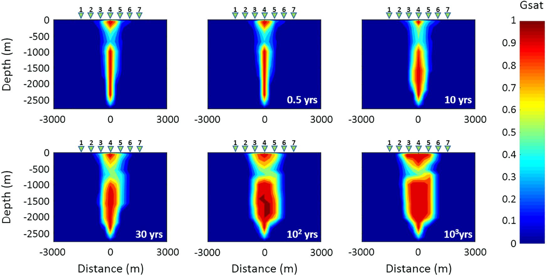
Figure 6. Time evolution of the gas saturation distribution related to Scenario I in the vertical section along the red line shown in Figure 3. The first panel of the sequence shows the initial gas saturation distribution. The green triangles 1–7 indicate the MT stations.

FIGURE 7

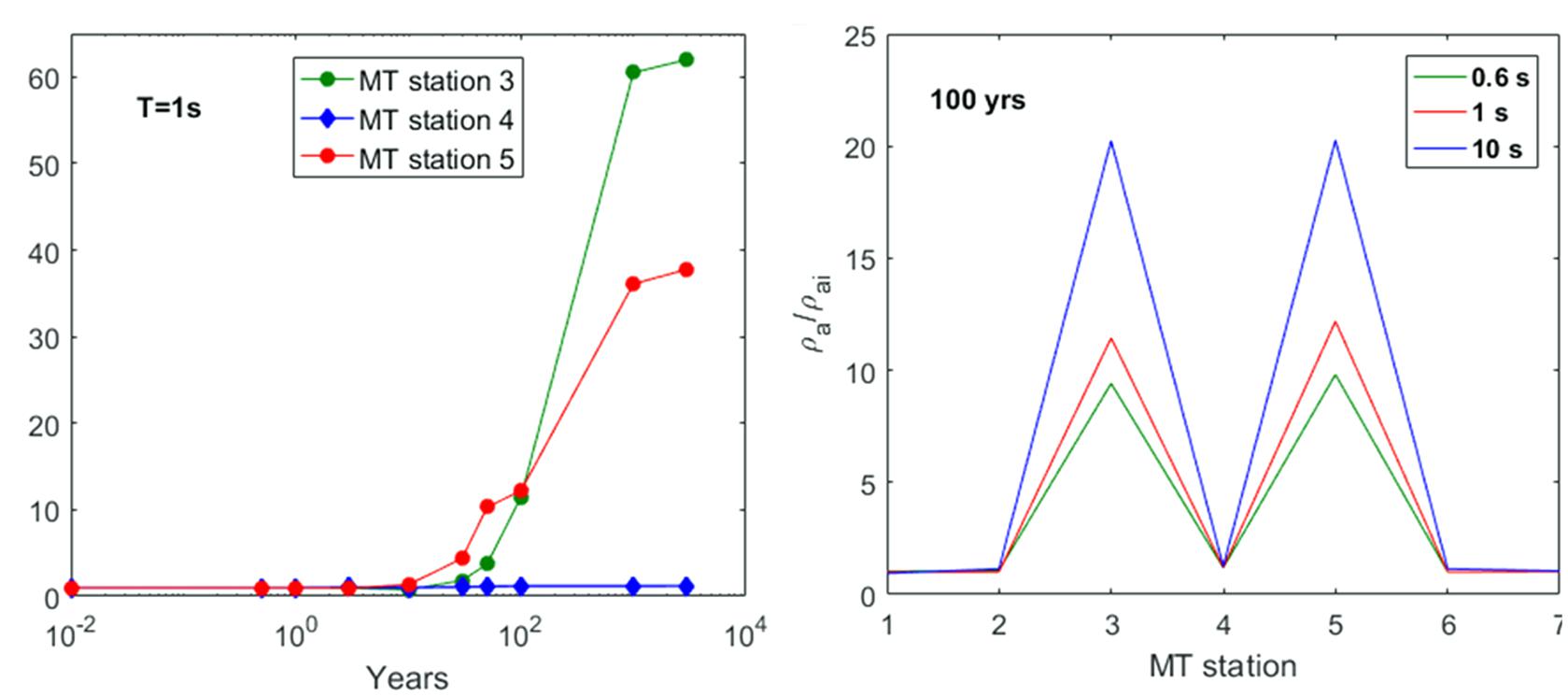
Figure 7. Scenario I. (A) Ratio between the synthetic apparent resistivity values (ρ_a) and the initial resistivity value (ρ_ai) estimated for the three central MT stations as a function of time at the fixed period T = 1 s. (B) Ratio between the synthetic apparent resistivity values (ρ_a) and the initial resistivity value (ρ_ai) estimated after a simulation time of 100 years for the seven MT stations at three fixed periods.

FIGURE 8

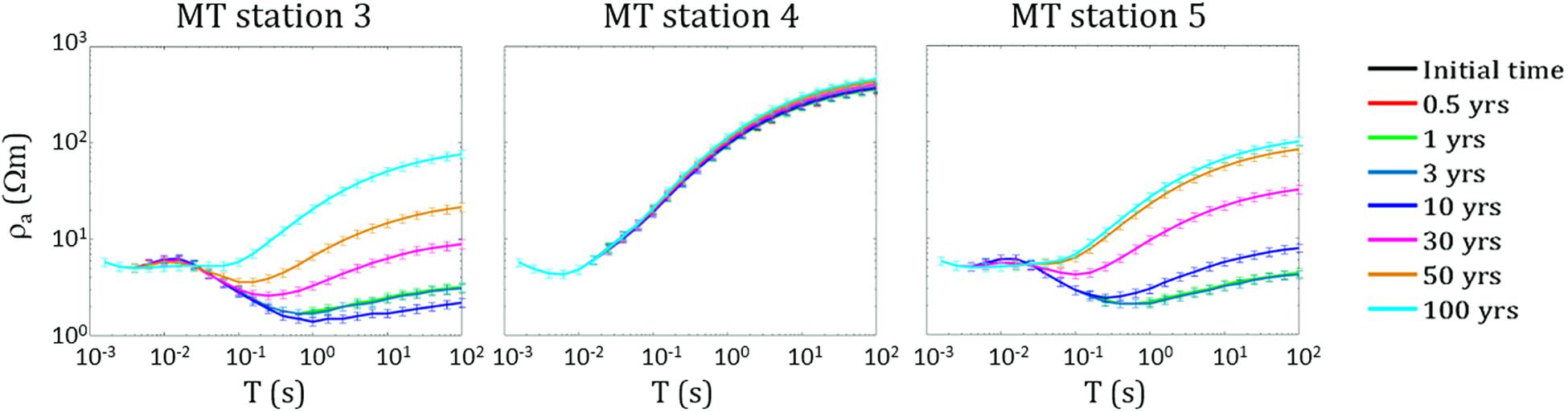
Figure 8. Scenario I. Apparent resistivity curves as a function of period T calculated for the three central MT stations at seven different simulation times.

Summarizing, if a hydrothermal system is involved exclusively by an increase of the fluid flow rate from the source, the variations of the parameters that affect the resistivity (i.e., temperature and gas saturation) are too slow to be appreciated through continuous MT observations within a time interval useful for monitoring purposes.

Scenario II: Effect of Permeability Increasing

The second hypothesized scenario assumes an increase in the permeability of the rocks that characterize the fluid upwelling zone above the hydrothermal system source. Several simulations have been performed by considering different increases of the permeability values assigned to the portion of the system indicated by the black dashed ellipse in Figure 3. For brevity, as an example we show the simulation results obtained for an increase in permeability of two orders of magnitude with respect to the original permeability distribution of the model assumed by Petrillo et al. (2013), which is characterized by values ranging from 1 × 10^–19 to 3.66 × 10^–14 m². The system evolution has been simulated for a time interval of 1 kyr. In particular, Figure 9 shows the temperature distribution obtained at different time steps over a span of 100 years. A decrease in the temperature values starts to be observed after 0.5 years in the central upwelling zone at depths between 250 and 1000 m b.g.l., as the effect of the permeability increase allows the entry of water from the surrounding rocks. Such a temperature decrease continues during the system evolution even if more slowly. As expected, the same area is also affected by a significant decrease in gas saturation which starts after 0.5 years and continues until complete saturation in water occurs after 10 years (Figure 10). It is therefore reasonable to assume that the observed changes in temperature and gas saturation produce significant variations in the resistivity distribution of the system, which can be revealed by variations in the MT response over time intervals useful for monitoring purposes. This hypothesis is confirmed by the results shown in Figure 11A, which displays, for the three central MT stations, the time variations of the ratio between the resistivities ρ_a and ρ_ai evaluated at period T = 1 s. As it can be seen, appreciable apparent resistivity decreases are observed after 6 months, which are more evident for the three central stations as shown in Figure 11B. In Figure 12, apparent resistivity curves for these stations are shown as a function of period at seven different simulation times. The curves show a similar trend for all the three stations, even if the largest and faster variations are observed at station 4.

FIGURE 9

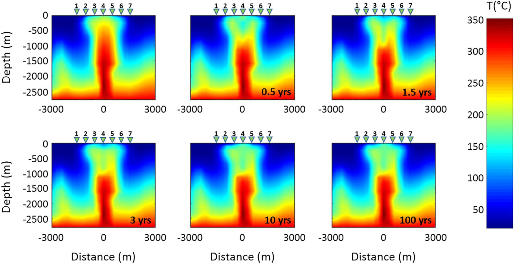
Figure 9. Time evolution of the temperature distribution related to Scenario II in the vertical section along the red line shown in Figure 3. The first panel of the sequence shows the initial temperature distribution. The green triangles 1–7 indicate the MT stations.

FIGURE 10

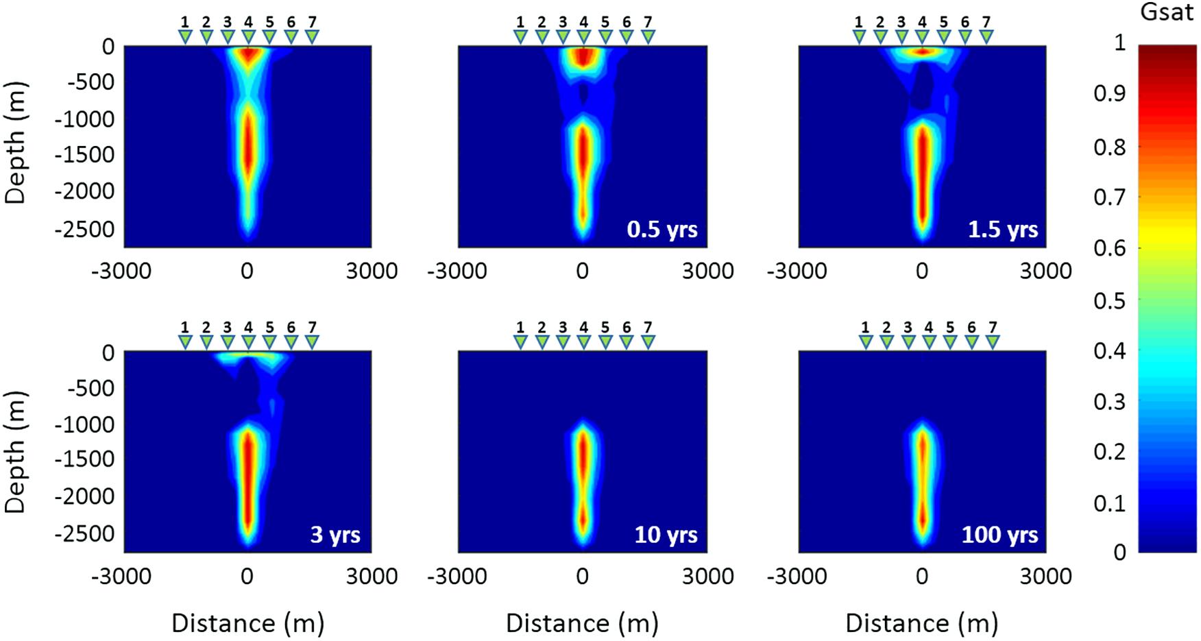
Figure 10. Time evolution of the gas saturation distribution related to Scenario II in the vertical section along the red line shown in Figure 3. The first panel of the sequence shows the initial gas saturation distribution. The green triangles 1–7 indicate the MT stations.

FIGURE 11

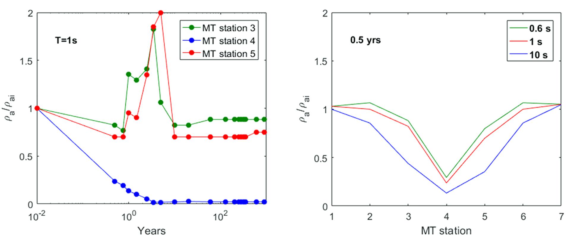
Figure 11. Scenario II. (A) Ratio between the synthetic apparent resistivity values and the initial resistivity value, estimated for the three central MT stations as a function of time at the fixed period T = 1 s. (B) Ratio between the synthetic apparent resistivity values and the initial resistivity value estimated after a simulation time of 0.5 years for the seven MT stations at three fixed periods.

FIGURE 12

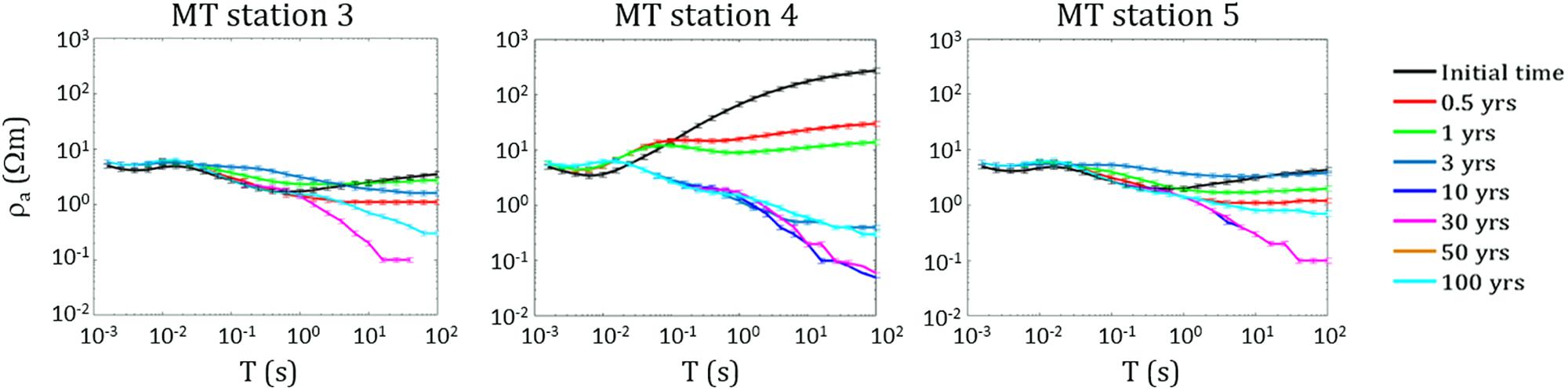
Figure 12. Scenario II. Apparent resistivity curves as a function of period calculated for the three central MT stations at seven different simulation times.

Summarizing, the performed simulations for the second scenario indicate that, as expected, the variation rate in temperature and, in particular, gas saturation is linked to the extent of the permeability increase. Specifically, appreciable variations are found starting from 6 months – for a permeability increase of 2–3 orders of magnitude – or from approximately 3 years – for a permeability increase of about half an order of magnitude, as highlighted in Figure 13, where the relative variation in gas saturation is shown for different increases in permeability value distribution. Correspondingly, the MT response at stations located in proximity of the area affected by permeability variations significantly changes after a time interval ranging from 6 months to 3 years (see Figure 12).

FIGURE 13

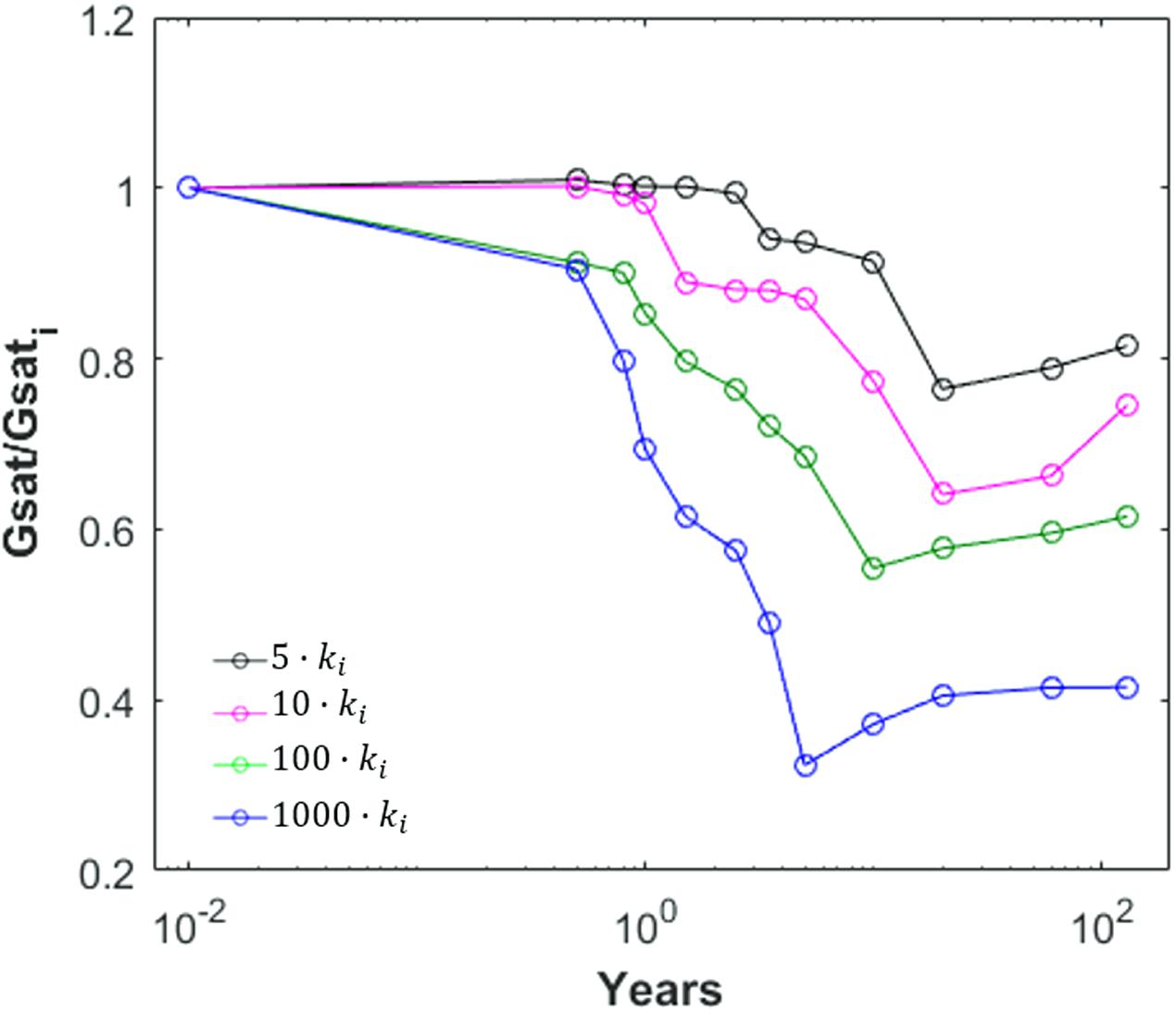
Figure 13. Time variation of the mean gas saturation related to Scenario II in the central upwelling zone (black dashed ellipse in Figure 3) normalized to its initial value for four different increases of the initial permeability values, k_i.

Conclusion

A sensitivity study aimed at estimating the effectiveness of continuous magnetotelluric observations for monitoring hydrothermal system dynamics has been presented. In particular, two possible evolution scenarios of a hydrothermal system have been assumed, corresponding to an increase in fluid flow rate from the system source and permeability of the rocks hosting the fluid upwelling zone, respectively. Several numerical simulations have been performed for each scenario and the MT response has been estimated at fixed time steps to assess the time intervals needed for observing significant variations in the apparent resistivity. The proposed approach has been applied to a 3D petrophysical model representative of the CF hydrothermal system and a modified form of the Archie’s law has been used to transform the distribution of values of porosity, temperature and water saturation into the electrical resistivity values. The simulation results related to the first scenario show variations in gas saturation and temperature too slow to be detected with continuous MT observations in a time interval suitable for monitoring purposes. Conversely, the simulations related to the second scenario show significant variations in the gas saturation distribution over a time interval ranging from 3 months to 3 years, which give rise to resistivity variations detectable by continuous MT observations in the same time interval. This result is promising for the monitoring of hydrothermal activity, as it proves the effectiveness of the MT method in identifying possible changes in the hydraulic parameters of a hydrothermal system likely related to changes in its dynamics. However, although the observed apparent resistivity variations related to the simulated scenarios are far greater than 10%, which is the error assumed for each impedance tensor estimate, robust filtering techniques for denoising MT signals must be applied to take into account the presence of heavy cultural noise on MT data collected in highly urbanized areas such as our test site. In addition, further studies are required to consider more complex scenarios including, for example, seasonal rainfalls, progressive increases of the dynamical variables of the system and presence of faults. Currently, the extension of the presented numerical modeling to 3D MT data sets is in progress as well as the installation of MT continuous stations in the CF hydrothermal area whose recordings could support this study.

Data Availability Statement

The datasets generated for this study are available on request to the corresponding author.

Author Contributions

RD designed the research. RD, RC, and EP analyzed and interpreted the data, and wrote the manuscript. RC performed the numerical simulations.

Conflict of Interest

The authors declare that the research was conducted in the absence of any commercial or financial relationships that could be construed as a potential conflict of interest.

The handling Editor declared a shared affiliation, though no other collaboration, with the authors RC, RD, and EP at the time of the review.

Acknowledgments

The authors acknowledge Zaccaria Petrillo for providing the petrophysical data useful to build the Campi Flegrei model and for helpful discussions. The authors thank the editor and the two reviewers for their valuable comments, which helped improving the manuscript.

References

Acocella, V. (2010). Evaluating fracture patterns within a resurgent caldera: Campi Flegrei, Italy. Bull. Volcanol. 72, 623–638. doi: 10.1007/s00445-010-0347-x

CrossRef Full Text | Google Scholar

Afanasyev, A., Costa, A., and Chiodini, G. (2015). Investigation of hydrothermal activity at Campi Flegrei caldera using 3D numerical simulations: extension to high temperature processes. J. Volcanol. Geother. Res. 299, 68–77. doi: 10.1016/j.jvolgeores.2015.04.004

CrossRef Full Text | Google Scholar

Aizawa, K., Kanda, W., Ogawa, Y., Iguchi, M., Yokoo, A., Yakiwara, H., et al. (2011). Temporal changes in electrical resistivity at Sakurajima volcano from continuous magnetotelluric observations. J. Volcanol. Geother. Res. 199, 165–175. doi: 10.1016/j.jvolgeores.2010.11.003

CrossRef Full Text | Google Scholar

Amatyakul, P., Boonchaisuk, S., Rung-Arunwan, T., Vachiratienchai, C., Wood, S. H., Pirarai, K., et al. (2016). Exploring the shallow geothermal fluid reservoir of Fang geothermal system, Thailand via a 3-D magnetotelluric survey. Geothermics 64, 516–526. doi: 10.1016/j.geothermics.2016.08.003

CrossRef Full Text | Google Scholar

Amoruso, A., Crescentini, L., and Sabbetta, I. (2014). Paired deformation sources of the Campi Flegrei caldera (Italy) required by recent (1980–2010) deformation history. J. Geophys. Res. 119, 858–879. doi: 10.1002/2013jb010392

CrossRef Full Text | Google Scholar

Archie, G. E. (1942). The electrical resistivity log as an aid in determining some reservoir characteristics. Pet. Trans. AIME 146, 54–62. doi: 10.2118/942054-G

CrossRef Full Text | Google Scholar

Bahr, K. (1988). Interpretation of the magnetotelluric impedance tensor: regional induction and local telluric distortion. J. Geophys. 62, 119–127.

Google Scholar

Bartel, B. A., Hamburger, M. W., Meertens, C. M., Lowry, A. R., and Corpuz, E. (2003). Dynamics of active magmatic and hydrothermal systems at Taal Volcano, Philippines, from continuous GPS measurements. J. Geophys. Res. 108:2475. doi: 10.1029/2002JB002194

CrossRef Full Text | Google Scholar

Bedrosian, P. A., Weckmann, U., Ritter, O., Hammer, C., Hübert, J., and Jung, A. (2004). “Electromagnetic monitoring of the Groβ Schönebeck stimulation experiment,” in Proceedings Jahrestagung der Deutschen Geophysikalischen Gessellschaft, Königstein, 64.

Google Scholar

Berrino, G., Corrado, G., Luongo, G., and Toro, B. (1984). Ground deformation and gravity changes accompanying the 1982 Pozzuoli uplift. Bull. Volcanol. 47, 187–200. doi: 10.1007/bf01961548

CrossRef Full Text | Google Scholar

Bibby, H. M., Caldwell, T. G., Davey, F. J., and Webb, T. H. (1995). Geophysical evidence on the structure of the Taupo Volcanic Zone and its hydrothermal circulation. J. Volcanol. Geother. Res. 68, 29–58. doi: 10.1016/0377-0273(95)00007-h

CrossRef Full Text | Google Scholar

Biggs, J., Ebmeier, S. K., Aspinall, W. P., Lu, Z., Pritchard, M. E., Sparks, R. S. J., et al. (2014). Global link between deformation and volcanic eruption quantified by satellite imagery. Nat. Commun. 5:3471. doi: 10.1038/ncomms4471

PubMed Abstract | CrossRef Full Text | Google Scholar

Byrdina, S., Vandemeulebrouck, J., Cardellini, C., Legaz, A., Camerlynck, C., Chiodini, G., et al. (2014). Relations between electrical resistivity, carbon dioxide flux, and self-potential in the shallow hydrothermal system of Solfatara (Phlegrean Fields, Italy). J. Volcanol. Geother. Res. 283, 172–182. doi: 10.1016/j.jvolgeores.2014.07.010

CrossRef Full Text | Google Scholar

Caldwell, T. G., Bibby, H. M., and Brown, C. (2004). The magnetotelluric phase tensor. Geophys. J. Int. 158, 457–469. doi: 10.1038/s41598-019-43763-w

PubMed Abstract | CrossRef Full Text | Google Scholar

Caliro, S., Chiodini, G., Moretti, R., Avino, R., Granieri, D., Russo, M., et al. (2007). The origin of the fumaroles of La Solfatara (Campi Flegrei, south Italy). Geochim. Cosmochim. Acta 71, 3040–3055. doi: 10.1016/j.gca.2007.04.007

CrossRef Full Text | Google Scholar

Caliro, S., Chiodini, G., and Paonita, A. (2014). Geochemical evidences of magma dynamics at Campi Flegrei (Italy). Geochim. Cosmochim. Acta 132, 1–15. doi: 10.1016/j.gca.2014.01.021

CrossRef Full Text | Google Scholar

Carbonari, R., Di Maio, R., Piegari, E., D’Auria, L., Esposito, A., and Petrillo, Z. (2018). Filtering of noisy magnetotelluric signals by SOM neural networks. Phys Earth Planet. Interiors 285, 12–22. doi: 10.1016/j.pepi.2018.10.004

CrossRef Full Text | Google Scholar

Cardellini, C., Chiodini, G., and Frondini, F. (2003a). Application of stochastic simulation to CO2 flux from soil: mapping and quantification of gas release. J. Geophys. Res. 108:2425.

Google Scholar

Cardellini, C., Chiodini, G., Frondini, F., Granieri, D., Lewicki, J., and Peruzzi, L. (2003b). Accumulation chamber measurements of methane fluxes: application to volcanic-geothermal areas and landfills. Appl. Geochem. 18, 45–54. doi: 10.1016/s0883-2927(02)00091-4

PubMed Abstract | CrossRef Full Text | Google Scholar

Chave, A. D., and Thomson, D. J. (2004). Bounded influence magnetotelluric response function estimation. Geophys. J. Int. 157, 988–1006. doi: 10.1111/j.1365-246x.2004.02203.x

CrossRef Full Text | Google Scholar

Chiodini, G., Caliro, S., Aiuppa, A., Avino, R., Granieri, D., Moretti, R., et al. (2011). First 13 C/12 C isotopic characterisation of volcanic plume CO₂. Bull. Volcanol. 73, 531–542. doi: 10.1007/s00445-010-0423-2

CrossRef Full Text | Google Scholar

Chiodini, G., Caliro, S., Cardellini, C., Granieri, D., Avino, R., Baldini, A., et al. (2010). Long-term variations of the Campi Flegrei, Italy, volcanic system as revealed by the monitoring of hydrothermal activity. J. Geophys. Res. 115::B03205. doi: 10.1029/2008JB006258

CrossRef Full Text | Google Scholar

Chiodini, G., Caliro, S., De Martino, P., Avino, R., and Gherardi, F. (2012). Early signals of new volcanic unrest at Campi Flegrei caldera? Insights from geochemical data and physical simulations. Geology 40, 943–946. doi: 10.1130/g33251.1

CrossRef Full Text | Google Scholar

Chiodini, G., Cioni, R., Guidi, M., Raco, B., and Marini, L. (1998). Soil CO2 flux measurements in volcanic and geothermal areas. Appl. Geochem. 13, 543–552. doi: 10.1016/s0883-2927(97)00076-0

CrossRef Full Text | Google Scholar

Chiodini, G., Paonita, A., Aiuppa, A., Costa, A., Caliro, S., De Martino, P., et al. (2016). Magmas near the critical degassing pressure drive volcanic unrest towards a critical state. Nat. Commun. 7:13712. doi: 10.1038/ncomms13712

PubMed Abstract | CrossRef Full Text | Google Scholar

Chiodini, G., Todesco, M., Caliro, S., Del Gaudio, C., Macedonio, G., and Russo, M. (2003). Magma degassing as a trigger of bradyseismic events: the case of Phlegrean Fields (Italy). Geophys. Res. Lett. 30:1434.

Google Scholar

Costa, A. (2006). Permeability-porosity relationship: a reexamination of the Kozeny-Carman equation based on a fractal pore-space geometry assumption. Geophys. Res. Lett. 33:L02318.

Google Scholar

Dakhnov, V. N. (1962). Geophysical Well Logging: The Application of Geophysical Methods; Electrical Well Logging. Golden, CO: Colorado School of Mines, 445.

Google Scholar

De Natale, G., Troise, C., Pingue, F., Mastrolorenzo, G., Pappalardo, L., Battaglia, M., et al. (2006). The Campi Flegrei caldera: unrest mechanisms and hazards. Geol. Soc. 269, 25–45. doi: 10.1144/gsl.sp.2006.269.01.03

CrossRef Full Text | Google Scholar

Di Maio, R., and Berrino, G. (2016). Joint analysis of electric and gravimetric data for volcano monitoring. Application to data acquired at Vulcano Island (southern Italy) from 1993 to 1996. J. Volcanol. Geother. Res. 327, 459–468. doi: 10.1016/j.jvolgeores.2016.09.013

CrossRef Full Text | Google Scholar

Di Maio, R., Mauriello, P., Patella, D., Petrillo, Z., Piscitelli, S., and Siniscalchi, A. (1998). Electric and electromagnetic outline of the Mount Somma-Vesuvius structural setting. J. Volcanol. Geother. Res. 82, 219–238. doi: 10.1016/s0377-0273(97)00066-8

CrossRef Full Text | Google Scholar

Di Maio, R., Patella, D., Petrillo, Z., Siniscalchi, A., Cecere, G., and De Martino, P. (2000). Application of electric and electromagnetic methods to the definition of the Campi Flegrei caldera (Italy). Ann. Geophys. 43, 375–390.

Google Scholar

Di Vito, M. A., Isaia, R., Orsi, G., Southon, J. D., de Vita, S., D’Antonio, M., et al. (1999). Volcanism and deformation since 12,000 years at the Campi Flegrei caldera (Italy). J. Volcanol. Geother Res. 91, 221–246. doi: 10.1016/s0377-0273(99)00037-2

CrossRef Full Text | Google Scholar

Di Vito, M. A., Lirer, L., Mastrolorenzo, G., and Rolandi, G. (1987). The 1538 Monte Nuovo eruption (Campi Flegrei, Italy). Bull. Volcanol. 49, 608–615. doi: 10.1038/srep32245

PubMed Abstract | CrossRef Full Text | Google Scholar

Didana, Y. L., Heinson, G., Thiel, S., and Krieger, L. (2017). Magnetotelluric monitoring of permeability enhancement at enhanced geothermal system project. Geothermics 66, 23–38. doi: 10.1016/j.geothermics.2016.11.005

CrossRef Full Text | Google Scholar

Didana, Y. L., Thiel, S., and Heinson, G. (2015). “Magnetotelluric imaging at Tendaho high temperature geothermal field in north east Ethiopia,” in Proceedings World Geothermal Congress 2015, Melbourne, VIC.

Google Scholar

Egbert, G. D. (1997). Robust multiple-station magnetotelluric data processing. Geophys. J. Int. 130, 475–496. doi: 10.1111/j.1365-246x.1997.tb05663.x

CrossRef Full Text | Google Scholar

Finizola, A., Sortino, F., Lénat, J. F., Aubert, M., Ripepe, M., and Valenza, M. (2003). The summit hydrothermal system of Stromboli. New insights from self-potential, temperature, CO2 and fumarolic fluid measurements, with structural and monitoring implications. Bull. Volcanol. 65, 486–504. doi: 10.1007/s00445-003-0276-z

CrossRef Full Text | Google Scholar

Geiermann, J., and Schill, E. (2010). 2-D magnetotellurics at the geothermal site at Soultz-sous-Forêts: resistivity distribution to about 3000 m depth. Comptes Rendus Geosci. 342, 587–599. doi: 10.1016/j.crte.2010.04.001

CrossRef Full Text | Google Scholar

Glover, P. W. (2016). Archie’s law-a reappraisal. Solid Earth 7:1157.

Google Scholar

Glover, P. W., Hole, M. J., and Pous, J. (2000). A modified Archie’s law for two conducting phases. Earth Planet. Sci. Lett. 180, 369–383. doi: 10.1016/s0012-821x(00)00168-0

CrossRef Full Text | Google Scholar

Gresse, M., Vandemeulebrouck, J., Byrdina, S., Chiodini, G., Revil, A., Johnson, T. C., et al. (2017). Three-dimensional electrical resistivity tomography of the solfatara crater (Italy): implication for the multiphase flow structure of the shallow hydrothermal system. J. Geophys. Res. 122, 8749–8768. doi: 10.1002/2017jb014389

CrossRef Full Text | Google Scholar

Heise, W., Caldwell, T. G., Bibby, H. M., and Bannister, S. C. (2008). Three-dimensional modelling of magnetotelluric data from the Rotokawa geothermal field, Taupo Volcanic Zone, New Zealand. Geophys. J. Int. 173, 740–750. doi: 10.1111/j.1365-246x.2008.03737.x

CrossRef Full Text | Google Scholar

Hersir, G. P., and Björnsson, A. (1991). Geophysical Exploration for Geothermal Resources, Principles and Application. Iceland: UNU-GTP.

Google Scholar

Hersir, G. P., and Árnason, K. (2009). Resistivity of rocks. Paper Presented at Short Course IV on Exploration for Geothermal Resources, organized by UNU-GTP, KenGen and GDC, at Lake Naivasha, Kenya.

Google Scholar

Hurwitz, S., Lowenstern, J. B., and Heasler, H. (2007). Spatial and temporal geochemical trends in the hydrothermal system of Yellowstone National Park: inferences from river solute fluxes. J. Volcanol. Geother. Res. 162, 149–171. doi: 10.1016/j.jvolgeores.2007.01.003

CrossRef Full Text | Google Scholar

Isaia, R., Marianelli, P., and Sbrana, A. (2009). Caldera unrest prior to intense volcanism in Campi Flegrei (Italy) at 4.0 ka BP: implications for caldera dynamics and future eruptive scenarios. Geophys. Res. Lett. 36:L21303. doi: 10.1029/2009GL040513

CrossRef Full Text | Google Scholar

Keller, G. (1967). “Supplementary guide to the literature on electrical properties of rocks and minerals,” in Electrical Properties of Rocks. Monographs in Geoscience, ed. G. V. Keller, (Boston, MA: Springer).

Google Scholar

Keller, G., and Frischknecht, F. (1966). Electrical Methods in Geophysical Prospecting. Oxford: Pergamon Press, 523.

Google Scholar

Ladanivskyy, B., Zlotnicki, J., Reniva, P., and Alanis, P. (2018). Electromagnetic signals on active volcanoes: analysis of electrical resistivity and transfer functions at Taal volcano (Philippines) related to the 2010 seismovolcanic crisis. J. Appl. Geophys. 156, 67–81. doi: 10.1016/j.jappgeo.2017.01.033

CrossRef Full Text | Google Scholar

Larnier, H., Sailhac, P., and Chambodut, A. (2016). New application of wavelets in magnetotelluric data processing: reducing impedance bias. Earth Planets Space 68:70.

Google Scholar

Legaz, A., Vandemeulebrouck, J., Revil, A., Kemna, A., Hurst, A. W., Reeves, R., et al. (2009). A case study of resistivity and self-potential signatures of hydrothermal instabilities, Inferno Crater Lake, Waimangu, New Zealand. Geophys. Res. Lett. 36:L12306.

Google Scholar

Lima, A., De Vivo, B., Spera, F. J., Bodnar, R. J., Milia, A., Nunziata, C., et al. (2009). Thermodynamic model for uplift and deflation episodes (bradyseism) associated with magmatic–hydrothermal activity at the Campi Flegrei (Italy). Earth Sci. Rev. 97, 44–58. doi: 10.1016/j.earscirev.2009.10.001

CrossRef Full Text | Google Scholar

Lowenstern, J. B., Smith, R. B., and Hill, D. P. (2006). Monitoring super-volcanoes: geophysical and geochemical signals at Yellowstone and other large caldera systems. Philos. Trans. R. Soc. Lond. A Math., Phys. Eng. Sci. 364, 2055–2072. doi: 10.1098/rsta.2006.1813

PubMed Abstract | CrossRef Full Text | Google Scholar

MacFarlane, J., Thiel, S., Pek, J., Peacock, J., and Heinson, G. (2014). Characterisation of induced fracture networks within an enhanced geothermal system using anisotropic electromagnetic modelling. J. Volcanol. Geother. Res. 288, 1–7. doi: 10.1016/j.jvolgeores.2014.10.002

CrossRef Full Text | Google Scholar

Mackie, R. L., and Madden, T. R. (1993). Three-dimensional magnetotelluric inversion using conjugate gradients. Geophys. J. Int. 115, 215–229. doi: 10.1111/j.1365-246x.1993.tb05600.x

CrossRef Full Text | Google Scholar

Moran, S. C., Zimbelman, D. R., and Malone, S. D. (2000). A model for the magmatic–hydrothermal system at Mount Rainier, Washington, from seismic and geochemical observations. Bull. Volcanol. 61, 425–436. doi: 10.1007/pl00008909

CrossRef Full Text | Google Scholar

Munoz, G. (2014). Exploring for geothermal resources with electromagnetic methods. Surveys Geophys. 35, 101–122. doi: 10.1007/s10712-013-9236-0

CrossRef Full Text | Google Scholar

Newman, G. A., Gasperikova, E., Hoversten, G. M., and Wannamaker, P. E. (2008). Three-dimensional magnetotelluric characterization of the Coso geothermal field. Geothermics 37, 369–399. doi: 10.1016/j.geothermics.2008.02.006

CrossRef Full Text | Google Scholar

Peacock, J. R., Mangan, M. T., McPhee, D., and Wannamaker, P. E. (2016). Three-dimensional electrical resistivity model of the hydrothermal system in Long Valley Caldera, California, from magnetotellurics. Geophys. Res. Lett. 43, 7953–7962. doi: 10.1002/2016gl069263

CrossRef Full Text | Google Scholar

Peacock, J. R., Thiel, S., Heinson, G. S., and Reid, P. (2013). Time-lapse magnetotelluric monitoring of an enhanced geothermal system. Geophysics 78, B121–B130.

Google Scholar

Peacock, J. R., Thiel, S., Reid, P., and Heinson, G. (2012). Magnetotelluric monitoring of a fluid injection: example from an enhanced geothermal system. Geophys. Res. Lett. 39:L18403. doi: 10.1029/2012GL053080

CrossRef Full Text | Google Scholar

Petrillo, Z., Chiodini, G., Mangiacapra, A., Caliro, S., Capuano, P., Russo, G., et al. (2013). Defining a 3D physical model for the hydrothermal circulation at Campi Flegrei caldera (Italy). J. Volcanol. Geother. Res. 264, 172–182. doi: 10.1016/j.jvolgeores.2013.08.008

CrossRef Full Text | Google Scholar

Platz, A., and Weckmann, U. (2019). An automated new preselection tool for noisy Magnetotelluric data using the Mahalanobis distance and magnetic field constraints. Geophys. J. Int. 218, 1853–1872. doi: 10.1093/gji/ggz197

CrossRef Full Text | Google Scholar

Portier, N., Hinderer, J., Riccardi, U., Ferhat, G., Calvo, M., Abdelfettah, Y., et al. (2018). Hybrid gravimetry monitoring of Soultz-sous-Forêts and Rittershoffen geothermal sites (Alsace, France). Geothermics 76, 201–219. doi: 10.1016/j.geothermics.2018.07.008

CrossRef Full Text | Google Scholar

Pruess, K. (1991). TOUGH2-A General-Purpose Numerical Simulator for Multiphase Fluid and Heat Flow. California, CA: Lawrence Berkeley Lab.

Google Scholar

Puskas, C. M., Smith, R. B., Meertens, C. M., and Chang, W. L. (2007). Crustal deformation of the Yellowstone-Snake River Plain volcano-tectonic system: campaign and continuous GPS observations, 1987–2004. J. Geophys. Res. 112:B03401. doi: 10.1029/2006JB004325

CrossRef Full Text | Google Scholar

Quist, A. S., and Marshall, W. L. (1968). Electrical conductances of aqueous sodium chloride solutions from 0 to 800.degree. and at pressures to 4000 bars. J. Phys. Chem. 72, 684–703. doi: 10.1021/j100848a050

CrossRef Full Text | Google Scholar

Rodi, W., and Mackie, R. L. (2001). Nonlinear conjugate gradients algorithm for 2-D magnetotelluric inversion. Geophysics 66, 174–187. doi: 10.1190/1.1444893

CrossRef Full Text | Google Scholar

Rosi, M., and Sbrana, A. (1987). Campi Flegrei, CNR Quad. Ric. Sci. 114:175.

Google Scholar

Rouwet, D., Bellomo, S., Brusca, L., Inguaggiato, S., Jutzeler, M., Mora, R., et al. (2009). Major and trace element geochemistry of El Chichón volcano-hydrothermal system (Chiapas, México) in 2006-2007: implications for future geochemical monitoring. Geofísica Int. 48, 55–72.

Google Scholar

Samrock, F., Grayver, A. V., Eysteinsson, H., and Saar, M. O. (2018). Magnetotelluric image of transcrustal magmatic system beneath the Tulu Moye geothermal prospect in the Ethiopian Rift. Geophys. Res. Lett. 45, 12847–12855. doi: 10.1029/2018GL080333

CrossRef Full Text | Google Scholar

Sasai, Y., Zlotnicki, J., Nishida, Y., Uyeshima, M., Yvetot, P., Tanaka, Y., et al. (2001). Evaluation of electric and magnetic field monitoring of Miyake-jima volcano (Central Japan): 1995-1999. Ann. Geophys. 44, 239–260.

Google Scholar

Schlumberger (2009). Log Interpretation Charts. Houston, TX: Schlumberger.

Google Scholar

Simpson, F., and Bahr, K. (2005). Practical Magnetotellurics. Cambridge: Cambridge University Press, 272.

Google Scholar

Siniscalchi, A., Tripaldi, S., Romano, G., Chiodini, G., Improta, L., Petrillo, Z., et al. (2019). Reservoir structure and hydraulic properties of the Campi Flegrei geothermal system inferred by audiomagnetotelluric, geochemical, and seismicity study. J. Geoph. Res. Solid Earth 124, 5336–5356.

Google Scholar

Stanley, W. D., Boehl, J. E., Bostick, F. X., and Smith, H. W. (1977). Geothermal significance of magnetotelluric sounding in the Eastern Snake River Plain-Yellowstone Region. J. Geophys. Res. 82, 2501–2514. doi: 10.1029/jb082i017p02501

CrossRef Full Text | Google Scholar

Tedesco, D., Pece, R., and Sabroux, J. C. (1988). No evidence of a new magmatic gas contribution to the Solfatara volcanic gases, during the Bradyseismic crisis at Campi Flegrei (Italy). Geophys. Res. Lett. 15, 1441–1444. doi: 10.1029/gl015i012p01441

CrossRef Full Text | Google Scholar

Todesco, M., Chiodini, G., and Macedonio, G. (2003). Monitoring and modelling hydrothermal fluid emission at La Solfatara (Phlegrean Fields, Italy). An interdisciplinary approach to the study of diffuse degassing. J. Volcanol. Geother. Res. 125, 57–79. doi: 10.1016/s0377-0273(03)00089-1

CrossRef Full Text | Google Scholar

Todesco, M., Rutqvist, J., Chiodini, G., Pruess, K., and Oldenburg, C. M. (2004). Modeling of recent volcanic episodes at Phlegrean Fields (Italy): geochemical variations and ground deformation. Geothermics 33, 531–547. doi: 10.1016/j.geothermics.2003.08.014

CrossRef Full Text | Google Scholar

Ussher, G., Harvey, C., Johnstone, R., and Anderson, E. (2000). “Understanding the resistivities observed in geothermal systems,” in Proceedings World Geothermal Congress 2000 Kyushu - Tohoku, Japan.

Google Scholar

Utada, H., Takahashi, Y., Morita, Y., Koyama, T., and Kagiyama, T. (2007). ACTIVE system for monitoring volcanic activity: a case study of the Izu-Oshima Volcano, Central Japan. J. Volcanol. Geother. Res. 164, 217–243. doi: 10.1016/j.jvolgeores.2007.05.010

CrossRef Full Text | Google Scholar

Volpi, G., Manzella, A., and Fiordelisi, A. (2003). Investigation of geothermal structures by magnetotellurics (MT): an example from the Mt. Amiata area, Italy. Geothermics 32, 131–145. doi: 10.1016/s0375-6505(03)00016-6

CrossRef Full Text | Google Scholar

Vozoff, K. (1990). Magnetotellurics: principles and practice. Proc. Indian Acad. Sci. Earth Planet. Sci. 99, 441–471.

Google Scholar

Wait, J. R. (1962). Theory of magnetotelluric fields. J. Res. Natl. Bur. Stand 66, 509–541.

Google Scholar

Wawrzyniak, P., Zlotnicki, J., Sailhac, P., and Marquis, G. (2017). Resistivity variations related to the large March 9, 1998 eruption at La Fournaise volcano inferred by continuous MT monitoring. J. Volcanol. Geother. Res. 347, 185–206. doi: 10.1016/j.jvolgeores.2017.09.011

CrossRef Full Text | Google Scholar

Weckmann, U., Magunia, A., and Ritter, O. (2005). Effective noise separation for magnetotelluric single site data processing using a frequency domain selection scheme. Geophys. J. Int. 161, 635–652. doi: 10.1111/j.1365-246x.2005.02621.x

CrossRef Full Text | Google Scholar

Zhang, J., Mackie, R. L., and Madden, T. R. (1995). 3-D resistivity forward modeling and inversion using conjugate gradients. Geophysics 60, 1313–1325. doi: 10.1190/1.1443868

CrossRef Full Text | Google Scholar

Zlotnicki, J., Boudon, G., Viodé, J. P., Delarue, J. F., Mille, A., and Bruere, F. (1998). Hydrothermal circulation beneath Mount Pelée inferred by self potential surveying. Structural and tectonic implications. J. Volcanol. Geother. Res. 84, 73–91. doi: 10.1016/s0377-0273(98)00030-4

CrossRef Full Text | Google Scholar

Zlotnicki, J., Vargemezis, G., Mille, A., Bruère, F., and Hammouya, G. (2006). State of the hydrothermal activity of Soufriere of Guadeloupe volcano inferred by VLF surveys. J. Appl. Geophys. 58, 265–279. doi: 10.1016/j.jappgeo.2005.05.004

CrossRef Full Text | Google Scholar