Mixing Layer Height Retrievals From MiniMPL Measurements in the Chiang Mai Valley: Implications for Particulate Matter Pollution

Introduction

The mixing layer (ML) is the turbulent layer of atmosphere adjacent to the earth’s surface which determines the vertical mixing of pollutants emitted at the surface by convective and mechanical turbulence (Stull, 1988; Seibert et al., 2000). The ML responds to variations in frictional drag, evapo-transpiration and sensible heat fluxes within the timescales of an hour or less. Development of the ML during the course of a day is governed by a variety of parameters, such as cloud cover, water vapor content, concentration of pollutants, strength of synoptic wind flow, soil moisture, nighttime cloud cover, and stratification in the free troposphere (Schween et al., 2014). During daytime the ML top represents the entrainment zone, which controls the mixing of air pollutants from the ML into the free troposphere. Thus, the thickness of the ML tends to aptly control the volume available for the dispersion of pollutants. Hence, an understanding of the diurnal and seasonal variations in the ML height is essential for discerning the mechanisms controlling the air quality, chemical processes and numerical modeling of the atmosphere (Monks et al., 2009).

The ML height can be determined with various indirect methods based on profile measurements using radiosonde, sodar, radar, LiDAR, ceilometers, etc (Seibert et al., 2000). In addition, surface flux measurements (such as sensible heat flux) can also be used to infer ML height (Haeffelin et al., 2012). Furthermore, a more comprehensive understanding of ML dynamics can be obtained by using an elastic LiDAR in combination with microwave radiometers and Doppler lidars, which can measure profiles of temperature and vertical wind speed, respectively (de Arruda Moreira et al., 2018). The high spatiotemporal resolution makes aerosol LiDAR techniques one of the most suitable measurement techniques for understanding ML evolution (Flamant et al., 1997). ML height detection from LiDAR profiles, being an almost direct measure of variations in aerosol concentration profiles, can reveal intricate features about the vertical structure of the atmosphere in the context with dispersal of pollutants (Yang et al., 2013). Using aerosols as a tracer, LiDAR backscatter profiles can be utilized for extracting the ML height, with a typical vertical resolution of meters and temporal resolution of seconds to minutes. Such studies can be very much useful in investigating the regional air quality issues (Boyouk et al., 2010). However, the ML estimations using LiDAR backscatter profiles assumes the main source of aerosols at the underlying surface and related activities, with the aerosols being uniformly mixed in the ML through turbulent mixing (Schween et al., 2014). In general the ML estimations based on aerosol backscatter work quite well during the daytime convective hours, whereas being highly uncertain in the transition period during the early morning and early evening hours due to the similar strength of aerosol gradient at the top of the residual layer and ground aerosol layer (Dang et al., 2019). During the night-time hours the ML height estimations from the backscatter profile correspond to either the top of the residual layer or the ML driven by mechanical mixing near the ground surface.

A variety of techniques for ML height detection has been suggested, which includes the application of a gradient technique on the range corrected signal (RCS) (Flamant et al., 1997; García-Franco et al., 2018) and the logarithm of the RCS (He et al., 2006), maximum of the RCS temporal variance (Hooper and Eloranta, 1986), wavelet analysis of the RCS profile (Cohn and Angevine, 2000), extended Kalman filter method (Lange et al., 2014), and the cubic root gradient of the RCS profile (Yang et al., 2017). Although fully automated, ML height detection is restricted by the limitations of various techniques (Yang et al., 2013; Ware et al., 2016) in clearly identifying different features in the lower troposphere. However, with more detailed studies on the evolution of the lower troposphere through continuous LiDAR measurements, the automated techniques have been advancing significantly over the past decade (Haeffelin et al., 2012; Dang et al., 2019).

For flat homogeneous terrain the ML variations have been investigated in detail (Stull, 1988). However, over mountainous terrain, the topography exerts its influence on the atmosphere, thus affecting the transport and mixing processes trough mountain waves, rotors, and thermally driven wind systems (Whiteman, 2000; Zardi and Whiteman, 2013; De Wekker and Kossmann, 2015). In context with a mountain valley, the role of the ML in confinement of air pollutants is further strengthened as a result of terrain induced restrictions on air flow and ventilation. Since, the valley atmosphere is strongly under the influence of valley and slope winds, thus continuous measurements of ML height variations can provide detailed insight into the processes controlling the valley atmosphere and forecasting air quality. ML height being one of the controlling factors for the dilution of the pollutants through vertical turbulent mixing (Geiß et al., 2017), thus, simultaneous measurements of ML height and atmospheric pollutant concentrations can provide a useful insight into their inter-dependence. De Wekker and Mayor (2009) investigated the various components of the valley atmosphere through scanning LiDAR, thereby illustrating the wide applicability of high resolution LiDAR measurements. Due to the stronger mixing over mountainous topography the aerosols are transported up to the aerosol layer (AL) height which is usually above the ML height, hence AL height is also an important parameter for air pollution studies in context with mountains. According to De Wekker et al. (2004) the LiDAR usually measures the AL height instead of ML height, depending primarily on the assumption of the equality between ML and AL which is prominently violated over mountainous topography. In this study we investigate the simultaneous assessment of the AL and ML height over the site based on the detailed analysis of 15 months of MiniMPL measurements.

Wang et al. (2015) investigated the aerosol vertical distribution and columnar properties over northern Thailand during the 2014 spring season as part of the 7-SEAS campaign. The LiDAR measurements obtained at the Doi Ang Khang station (1536 m above mean sea level) illustrated large amplitude in aerosol diurnal variations mainly dominated by ML height variations extending up to 5 km above sea level in the daytime. Moreover, during night-time the aerosol loading declined over the station as a result of strong westerly winds. The measurement station, thus being in the free troposphere during the nighttime, with aerosol reaching the station as the ML evolves during the daytime hours. Hence, ML height variations over the valley can have strong influence on air pollutants concentration within the valley, thus highlighting the need for continuous ML height measurements at the valley floor.

The prime objective of this study is to investigate the variations in ML height based on the analysis of continuous MiniMPL measurements during April 2017 to June 2018 in the mountain valley of Chiang Mai. Section “Observational Site and Instrumentation” provides a brief description of the observational site, details on the MiniMPL and PM measurements; section “Data Analysis” discusses the methodology of the extraction of ML and AL height information from continuous MiniMPL measurements; section “Results” presents the results on variations in the ML and AL heights along with its influence on the variation in the PM concentrations, and finally the concluding remarks are provided in section “Discussion.” Local time (LT) refers to UTC + 7:00 for the analysis presented in this study.

Observational Site and Instrumentation

The observational site is located at 18.852°N and 98.958°E, 332 m AMSL at the Princess Sirindhorn AstroPark of the National Astronomical Research Institute of Thailand (NARIT), Chiang Mai. Chiang Mai is the largest city in Northern Thailand located within a mountain valley as depicted in Figure 1. The valley is oriented along the north-south direction surrounded by mountains higher than 1 km on all sides. The observational site is situated at the North-western side of the valley floor. On a regional scale February, March, and April are the driest months of the year with major events of crop residue burning and forest fires resulting in polluted haze episodes in the valley. The month of May and June are accompanied with the onset of the southwest monsoon and some severe thunderstorms, gradually transitioning into intermittent monsoon rain spells from July to October. In the month of November, December and January, mostly cloud free sky conditions are prevalent with few instances of valley fog.

FIGURE 1

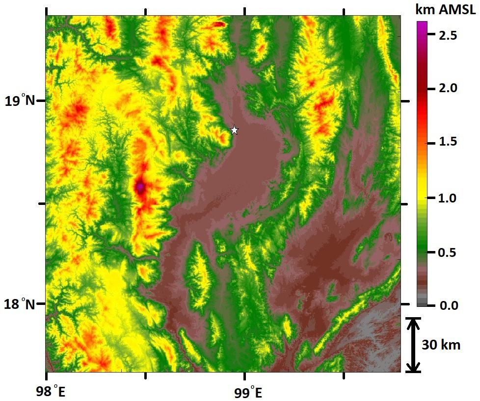
Figure 1. Topography of the region surrounding the valley of Chiang Mai in Northern Thailand. The location of the MiniMPL measurements site is highlighted by the star in white color.

For this study, the active remote sensing measurements were carried out with the Sigma Space Mini-Micropulse LiDAR (MiniMPL) as shown in Figure 2. The MiniMPL was made operational on April 11, 2017 and since then it has been providing continuous measurements of backscatter profiles of the lower atmosphere. The measurements for the current site were conducted until October 24, 2018, and since then the MiniMPL has been relocated to another locations in Chiang Mai Province. The MiniMPL is the compact version of the standard MPL which is part of the NASA MPLNET LiDAR network (Ware et al., 2016). The system is provided with an automated web switch regulated by the temperature of the enclosure of the MiniMPL unit. The enclosure temperature is maintained by the air-conditioning unit which maintains the continuous monitoring of the atmosphere, but on a few occasions such as power failure or high air temperatures during the noontime, the instrument was switched off and later turned on under suitable operating conditions.

FIGURE 2

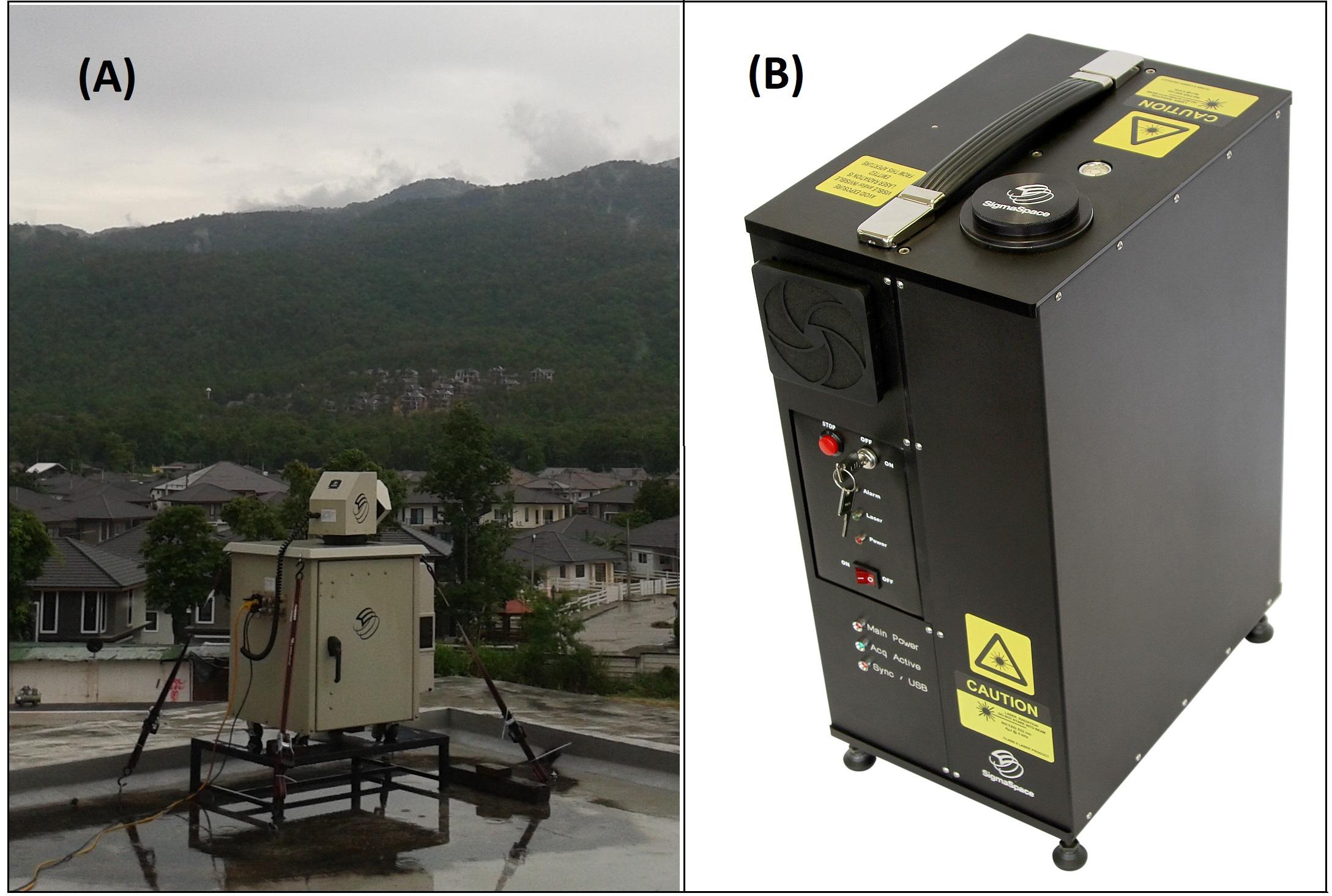
Figure 2. (A) Photograph of the complete MiniMPL unit installed at the NARIT Astro Park in Chiang Mai. (B) Photograph of the MiniMPL transceiver unit.

The MiniMPL is incorporated with an Nd:YAG laser as the light source, sending pulses of 532 nm LASER shots in an expanded/collimated beam of 80 mm diameter vertically propagating upward into the atmosphere at a pulse repetition frequency of 2.5 kHz. The backscattered photon count profile is recorded at every 30 s with a vertical range resolution of 30 m. The backscattered signal is recorded along two perpendicular planes (co-polarized and cross-polarized) of polarization. The MiniMPL uses a coaxial design with the transmitter and receiver field of view (FOV) overlapping from range zero, the receiver FOV being 220 μrad. The receiver uses a pair of narrowband filters with bandwidth less than 200 pm to reject the majority of solar background noise. More intricate details of the MiniMPL are provided in enlisted in Table 1.

TABLE 1

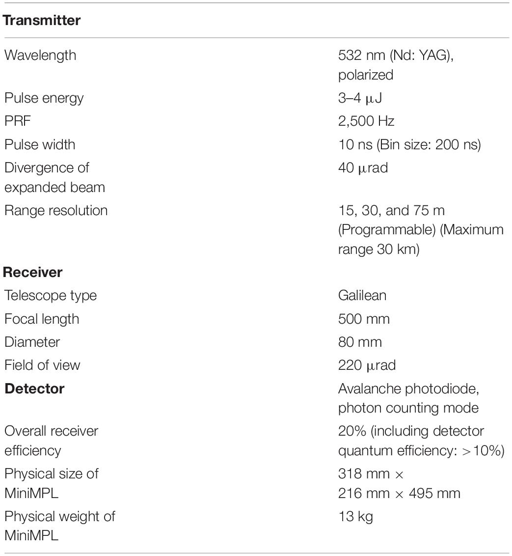
Table 1. Operating characteristics of the MiniMPL at NARIT.

The particulate matter (PM) concentration data (PM_2.5 and PM₁₀) along with the other meteorological measurements was acquired from the Pollution Control Department (PCD) of Thailand air quality monitoring station located at the City Hall 35T (18.841°N and 98.970°E), Chiang Mai (Macatangay et al., 2017). At the PCD station, the PM concentrations are measured with the tapered element oscillating microbalance (TEOM) Series 1400a (Rupprecht & Patashnick, United States) which utilizes the inertial mass weighing principle (Chantara, 2012; Jeensorn et al., 2018). The air quality monitoring station (City Hall 35T, Chiang Mai) is located within an aerial distance of less than 2 km from the MiniMPL site. The measurements of PM concentration are available with a temporal resolution of 1 h.

Data Analysis

The analysis of the MiniMPL measurements is primarily based on the normalized relative backscatter [NRB(r)] profiles which are obtained from the raw MiniMPL profiles [Raw(r)] after incorporating the dead time correction [D(r)], afterpulse correction [AP(r)], background correction (B), range correction (r²), overlap correction [O(r)] and energy normalization (E) as summarized below:

$$\mathrm{NRB}(\mathrm{r})=\frac{\text{[}(\text{Raw}\left(\text{r}\right)\mathrm{D}\left(\text{r}\right)-\mathrm{AP}\left(\text{r}\right)-\mathrm{B}]{\mathrm{r}}^2}{\text{O}\left(\text{r}\right)\mathrm{E}}$$

Despite of the MiniMPL being a coaxial system the overlap corrections incorporates the over-attenuation by range square correction on the near field signal. Since, in the near field the raw signal does not attenuate as described by the inverse range squared law, the overlap calibration file corrects for the over corrected near field signal by range square correction. The overlap calibration file is created by comparing the signal from overlap corrected (Standard LiDAR) and uncorrected (Test LiDAR) MiniMPL. The correction and calibration files were provided by Sigma Space Corporation during the time of installation of the instrument at the site.

For the analysis presented in this study the ML height is estimated based on the maximum negative gradient in the NRB profile along with a modified wavelet transform (Brooks, 2003; García-Franco et al., 2018) technique for minimizing the noise. In the algorithm, firstly the height of largest negative gradient is estimated and assessed for the possibility of a floor or false detection based on rapid change in ML height between two adjacent time-steps. If the gradient method based ML height is identified as false, a second estimate of ML height is made using the wavelet transform method with iteratively narrowing dilation. To increase the likelihood of correct ML detection, the retrieval of ML heights was constrained between 120 and 4,000 m with rate of change less than 2.4 km hr^–1. The algorithm finally excludes the floor or false detections and in case of rapid change in adjacent ML estimations the arithmetic mean of two methods is calculated as the ML height. The utilization of two methods in combination for the ML detection is quite useful to overcome the shortcomings of individual methods in the automated ML height analysis of large datasets with complex signal structure conditions caused by multiple aerosol layers, clouds, and noise (Dang et al., 2019). The cloud layers are detected based on a Sigma Space Corporation proprietary wavelet transform method partially based on a signal-to-noise ratio (SNR) threshold method. If a cloud is detected in the LiDAR profile, only values below the cloud base are used in the estimation of ML height. The screening of cloud-perturbed profiles and manual quality assurance to avoid upper aerosol layers (such as residual layers and nocturnal stable boundary layers) based on Yang et al. (2013) has also been incorporated in the analysis. The Signal-to-Noise ratio (SNR) was also incorporated in the analysis by screening out the data bins with SNR < 1.3 within each backscatter profile (Schween et al., 2014). The ML estimations during the period of fog, clouds or precipitation within the ML were also excluded from the analysis. Table 2 summarizes the number of observed and screened-in datasets for each month, which has been analyzed for understanding ML variations. Considering the dynamic state of the ML over mountainous topography (Singh et al., 2016) the backscatter profiles were averaged for every 15 min for extracting the ML height. The AL height has been estimated based on semi-objective method (De Wekker et al., 2004) for every 15 min and compared with the ML height measurements on similar temporal scales.

TABLE 2

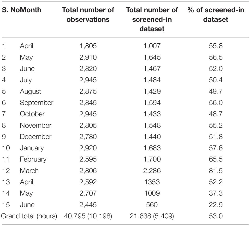
Table 2. Mini–micro pulse LiDAR 15 min average profiles statistics for the ML height analysis during April 2017 to June 2018.

Results

The analyzed MiniMPL aerosol profiles with successful detection of the ML height were statistically investigated to further extract a clearer picture of daily variations and monthly averaged diurnal cycles of ML evolution during April 2017 to June 2018. Figure 3 depicts the MiniMPL derived ML and AL height plotted over the range time intensity plot of NRB co-polarized backscatter retrievals for four consecutive days (February 28 to March 3, 2018). As clearly depicted, the ML height estimations (with the methodology and screening criterions described in section “Data Analysis”) are physically reasonable, with distinct diurnal variations for each day. Since, the AL represents the maximum vertical extent of aerosol transport (De Wekker and Kossmann, 2015), whereas the ML represents the extent of turbulent mixing, the ML and AL heights are of similar magnitude during the afternoon hours, however, ML estimations during the night-time hours are quite low as compared with AL height. Further statistics of variations over various temporal scales are discussed in the following subsections.

FIGURE 3

Figure 3. Estimated ML height (cyan circles) and AL height (purple circles) from the MiniMPL measurements during four consecutive days from February 28 to March 3, 2018 (00–24 LT). The background image is the normalized relative backscatter (NRB) of the co-polarized signal with 15 min temporal resolution (x-axis) and 30 m vertical resolution (y-axis).

Monthly Mean and Diurnal Variations

Figure 4 illustrates the monthly averaged diurnal cycles of ML height variability from April 2017 to June 2018. On average the ML height rises up to 2.5 km during the months of April to September attaining peak magnitudes at around 15 LT. A decrease of 0.5 km in the peak magnitude of ML height is observed in the months of October to December with higher ML heights in the night time. In the months of January and February the amplitude of diurnal variations is further reduced with the peak magnitude of the ML height being 1.5 km. From the analysis of monthly average diurnal variations in the ML height, the variations can be classified into three stages of evolution:

1. 09–15 LT time of gradual growth in ML thickness,

2. 15–19 LT time of rapid decrease in ML height, and

3. 20–09 LT time of small variations pertaining to stable ML height during night time and morning hours.

FIGURE 4

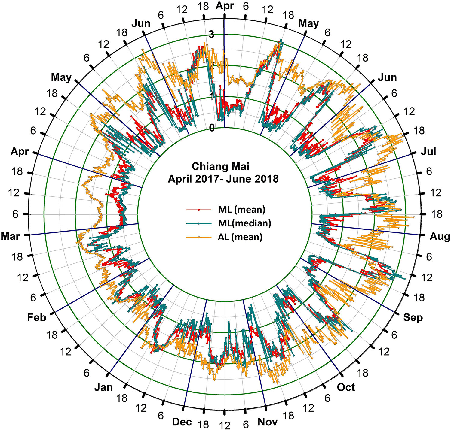
Figure 4. Polar plot for monthly mean diurnal variations in the 15-min binned mean, median of ML and mean AL height measurements for from April 2017 to June 2018. The polar plot is sectioned angularly into 15 sectors of 24° each, thus providing a composite overview of the monthly mean diurnal cycle during April 2017 to June 2018. The radial distance from the center represents the height above ground level in km.

Usually the ML height over flat terrain attains its maximum height between 12 and 13 LT (Stull, 1988). However, in this study of ML height evolution over a mountain valley, the growth of the ML height is gradual and extended up to 15 LT. The extended and gradual growth of ML thickness is due to the delay in the reversal of slope and valley winds. Similar lag in the ML maxima was also observed in the Kathmandu valley (Mues et al., 2017). Also, the higher night time ML height during October to February is due to the formation of stable valley inversions which results in the formation of a thicker residual layer as compared to the ML over flat ground. In general, the ML height evolution in mountain valleys is dominated by sources of heat which are the turbulent heat flux from the valley floor, the subsiding valley inversion (Kuwagata and Kimura, 1995), and the heating from the valley sidewall by slope wind recirculation (De Wekker and Kossmann, 2015).

Two distinct phases of ML height evolution are observed in the months of January and February with the first evolutionary phase from 06 to 09 LT and the second phase from 12 to 15 LT. The decrease in ML height from 09 to 12 LT is due to the destruction of the night time inversion over the valley. Usually during calm wind conditions of the morning hours, the down-valley winds in the remaining elevated valley inversions are eroded from the ground surface with the onset of up-valley winds, which can result in the evolution of ML for a short period of time (Eigenmann et al., 2009). During the month of March the diurnal evolution of the ML is strongly inhibited, confining the ML to 0.5 km from 06 to 15 LT; however, a weak evolutionary phase is observed from 15 to 20 LT. The strong confinement of ML during March could be due the formation of a thick haze layer over the valley as a result of crop residue burning and forest fires, despite the burning ban imposed by the local authorities during the dry season. The haze layer usually becomes thicker as a result of interplay between synoptic weather conditions and mountain meteorology.

ML_max and ML_min Variations

To investigate the variations in ML height, the dataset (April 2017 to June 2018) of screened ML height was classified into daytime (12–15 LT) and night time (00–03 LT) periods based on the statistical analysis of ML height variations. Such a classification can be useful to represent the characteristic maximum and minimum ML height of each day (Yang et al., 2013). For each day the daytime maximum ML height is stored as ML_max and the night time minimum ML height is stored as ML_min. Figure 5 shows an overview of the ML_max (triangles) and ML_min (circles) time series. To obtain an average picture of the variation in ML_max and ML_min, a 5-day moving average was also estimated, bringing out an interesting feature of periodic variations in ML_max. The maximum ML height was found to undergo periodic oscillations (approximate time period of 15 days) during April to September, varying between 2.5 and 3.5 km. The periodic oscillations in the ML_max could be associated with regular variations in synoptic conditions (He et al., 2013) over the region, and would be investigated in more detail in another study. The averaged ML_max reached maximum values of up to 4.0 km in the month of June to August; decreasing gradually from September until March. The few instances of almost equal magnitudes of ML_max and ML_min in the months of December to March are attributed to days with strong inversion layers forming over the valley suppressing daytime evolution of ML height during this cold period. As a result of the strong inversions, the residual layer is detected as the ML height instead of the weaker surface based inversion during night-time. Intense haze conditions over Chiang Mai Valley are usually observed (in particular during the burning/forest fire months of February and March) for the days during which the evolution of ML is inhibited during daytime.

FIGURE 5

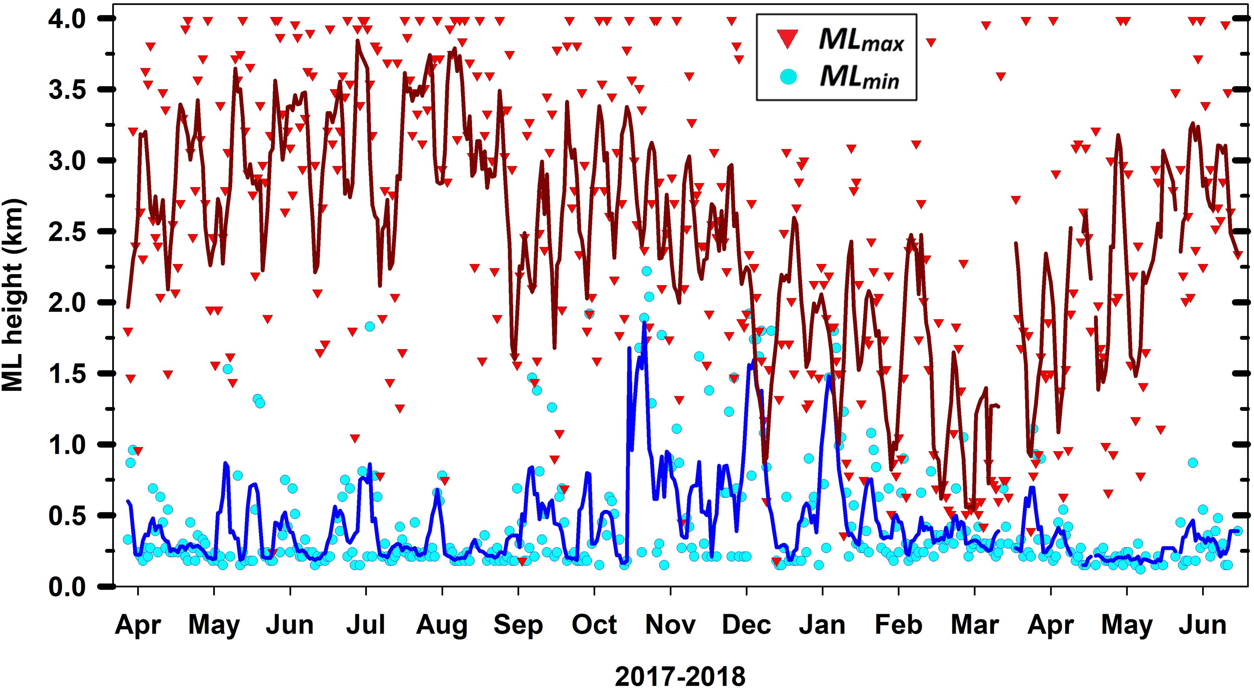
Figure 5. Variations in the 15-min binned daytime maximum (triangles) and night-time minimum (circles) ML height measurement April 2017 to June 2018. The solid line represents a 5-day centered moving average for the daytime maximum (solid red line) and night-time minimum (solid blue line) ML height measurements.

Rates of ML Growth and Decay

Based on the average monthly diurnal variations, the mean hourly growth rate of the ML height is estimated for every three consecutive months of the observational period. Usually positive growth rates (of the order of 0.21 km hr^–1) are observed from 06 to 15 LT. The ML decay starts always after 15 LT attaining negative growth rate (typically of the order of 0.38 km hr^–1) from 15 to 21 LT. From the analysis, the distinct and consistent transition from positive to negative growth rate of ML at 15 LT is observed. Interestingly, from October to March the growth rate oscillates between positive and negative values from midnight to noontime hours (00–12 LT), representing the interplay between mountain valley winds and subsiding valley inversions.

Ventilation Coefficient

Ventilation coefficient is an essential parameter for simultaneous quantification of vertical dispersion and advection in context with air pollution studies (Zhu et al., 2018). Based on the ML height and wind speed measurements the monthly average ventilation coefficient is calculated to gain further insight into the horizontal and vertical mixing capacity of the lower atmosphere (Tang et al., 2015; Mues et al., 2017). The monthly averaged yearly variations of wind speed and ventilation coefficient are depicted in Figure 6. The wind speed measurements were obtained from the collocated weather station at the site along with the MiniMPL. Due to a technical issue with the weather station the wind speed measurements were unavailable after April 16, 2018, therefore the ventilation coefficient for April 2018 was based on measurements of wind speed and ML measurements up to April 15, 2018. The ventilation coefficient is highest over the valley during the months of April, May, and June with magnitudes above 3000 m² s^–1 during the afternoon hours, from July to December the magnitudes of ventilation coefficient remain between 1000 and 3000 m² s^–1 in the afternoon hours. In the month of January and February the ventilation coefficient is further reduced in the daytime hours, with magnitudes marginally above 1000 m² s^–1 for 2–3 h of the day. Interestingly, the lowest magnitudes of ventilation coefficient (below 1000 m² s^–1) are observed during the month of March with the smallest amplitude of diurnal cycle. On average the very low values of ventilation coefficient are observed in the night-time hours due to the low wind speed along with the low ML height, thus indicating the capacity of local sources of air pollution within the valley in controlling the concentration air pollutants.

FIGURE 6

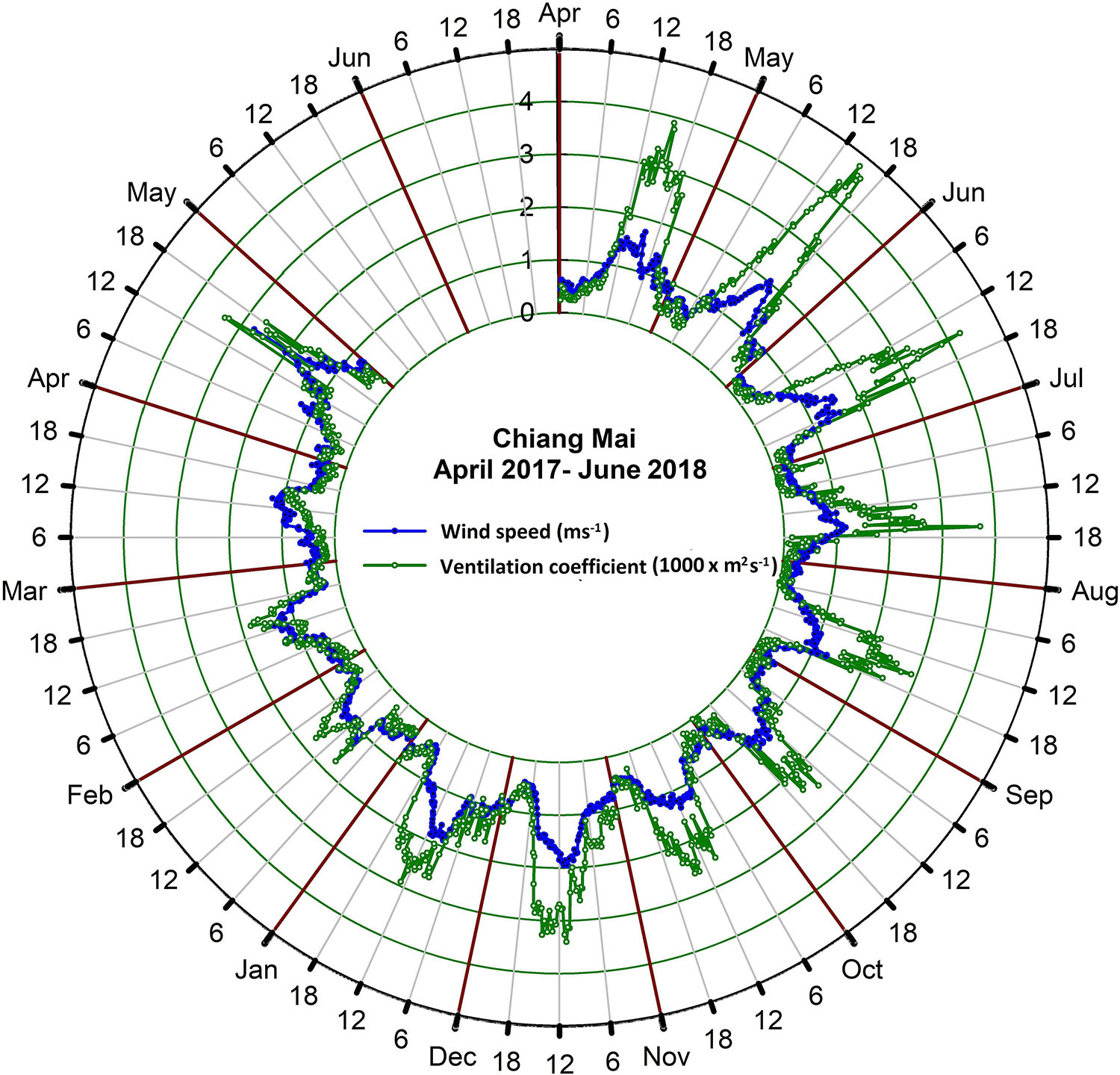
Figure 6. Polar plot for monthly mean diurnal variations in the 15-min binned mean of wind speed and ventilation coefficient from April 2017 to June 2018. The polar plot is sectioned angularly into 15 sectors of 24° each, thus providing a composite overview of the monthly averaged diurnal cycle during April 2017 to June 2018. The radial distance from the center represents the wind speed intensity (m s^{– 1}) and ventilation coefficient (1000 × m² s^{– 1}).

Particulate Matter Concentration Variations

The annual variations of the daily averaged PM concentrations from air quality monitoring station 35T measured during January 2017 to June 2018 are depicted in Figure 7, along with the monthly accumulated rainfall data, providing a clear overview of the haze season in the valley during February to April. The PM_2.5 (PM₁₀) concentrations remain below 20 μg m^–3 (40 μg m^–3) from May to October, being primarily controlled by the wash-out effect of the precipitation. From November onward the PM concentrations escalate gradually to higher concentrations. During the year 2017 and 2018, the PM_2.5 concentration exceeded the Thailand ambient air quality daily standard of 50 μg m^–3 (24-h average) on a total of 59 and 58 days, respectively at air quality monitoring station 35T. The months of February, March and April being the active months affected by forest fires and crop residue burning and weaker ventilation of the valley atmosphere result in sustaining PM_2.5 (PM₁₀) concentrations above 30 μg m^–3 (50 μg m^–3) throughout the dry season. Specifically, lowest ventilation coefficient and subsequently highest concentration of PM_2.5 and PM₁₀, were observed in the month of March 2018 indicating the clear role of ventilation affecting pollutant accumulation within the valley.

FIGURE 7

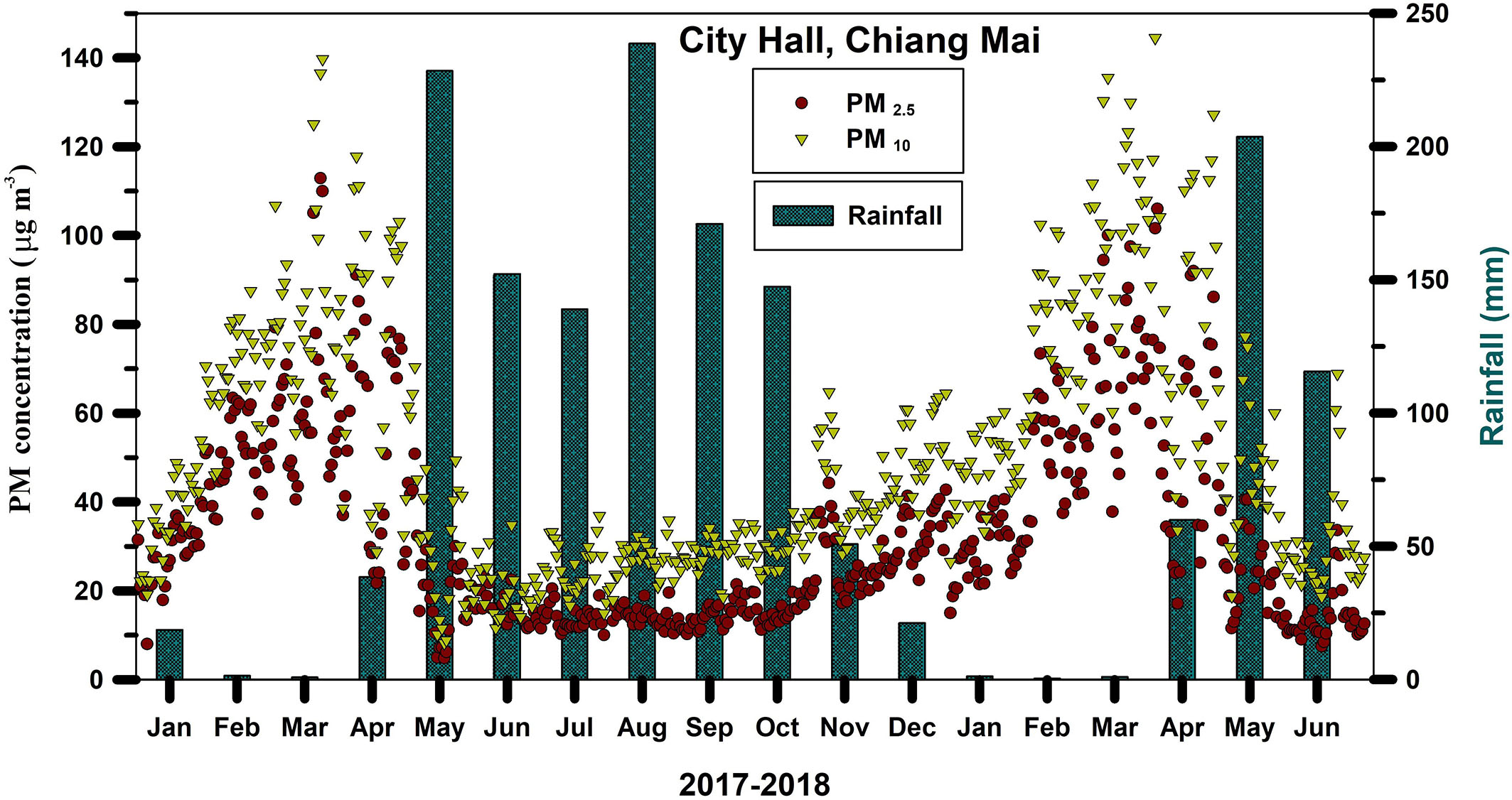
Figure 7. Daily mean values of PM (PM_2.5 and PM₁₀) concentrations and monthly accumulated rainfall measurements from the Pollution Control Department (PCD) air quality monitoring station at City Hall (35T), measured from January 2017 to June 2018.

In order to understand the effect of the variations in the ML height on the dilution of the PM concentrations in the valley of Chiang Mai, the monthly averaged diurnal variations in PM concentrations and ML height are analyzed. A clear reduction in the PM concentration is observed at the time corresponding to the increase in the ML height for the month of February, March, and April 2018, as depicted in Figures 8A–C. To further quantify the correlation between ML height and PM concentration, the simultaneous hourly measurements of the PM concentrations and the MiniMPL measured ML height are analyzed during the daytime hours (0700 to 1800 LT). A strong anti-correlation was confirmed during the dry season, with the Pearson correlation coefficient for PM_2.5 (PM₁₀) being –0.31 (–0.27); –0.48 (–0.51) and –0.56 (–0.55) during February, March, and April 2018, respectively, as depicted in Figures 8D–F, thereby, confirming the role of ML evolution in the dilution of PM concentration. Similarly, anti-correlation was also observed during April 2017. Interestingly the ML evolution was strongly inhibited on 21 days in March 2018, with daytime average ML height below 1 km and an average PM_2.5 (PM₁₀) concentration of more than 75 μg m^–3 (100 μg m^–3). Such high concentration of PM could have resulted in the enhancement of the stability of ML, thereby resulting in the suppression of ML evolution and further intensification of PM concentrations near ground surface. In contrast, during other months of the year (May to January) the dependency of PM concentrations on ML height is disguised (Pearson correlation coefficient < –0.10) as a result of regular events of precipitation.

FIGURE 8

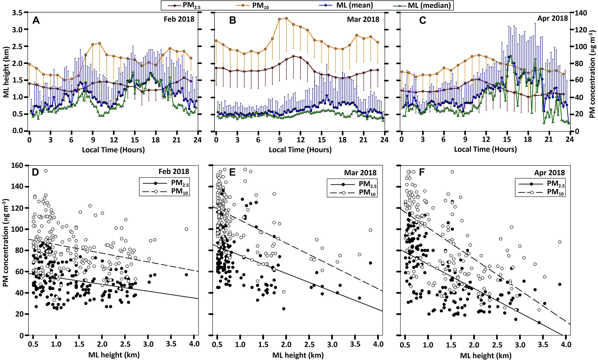
Figure 8. (A–C) Monthly averaged diurnal variations of PM (PM_2.5 and PM₁₀) concentrations along with the variations in mean and median of ML height for the month of February, March, and April 2018; (D–F) scatter plots of the hourly measurements of PM (PM_2.5 and PM₁₀) concentrations vs. the ML height for the month of February, March, and April 2018.

Discussion

The ML characteristics primarily define the dispersion, transport, transformation, and deposition of the air pollutants in the atmosphere. Lower ML heights are usually associated with higher PM concentrations near ground surface and vice-versa, although this relation is not always very significant and sometimes opposite as well (Geiß et al., 2017). Based on continuous MiniMPL measurements from April 2017 to June 2018, ML height variations were investigated in context with PM concentration variations over the valley of Chiang Mai. The analysis provided an overview of monthly averaged diurnal variations in the ML height, AL Height, ML_max, ML_min, ML growth rate, and ventilation coefficient providing a qualitative insight into the interplay of various processes controlling the valley atmosphere. Distinct diurnal cycles of ML and AL height evolution were observed from April to December with AL being always higher than ML with minimum difference during the afternoon hours. In the months of January and February, two phases of ML height evolution were observed with the daytime ML height remaining below 2 km. The consistent feature of the gradual evolution of ML height extending up to 15 LT, and decaying afterward is observed for all months except for March 2018. The daytime evolution of ML and AL was least prominent during March, along with the lowest magnitude of daytime ventilation coefficient, thus resulting in the strongest confinement of pollutants within the valley. The significant impact of the ML height on PM concentrations was observed during the dry season from February to April (Pearson coefficient ≈ –0.50), implying the role of ML height in the vertical mixing of the pollutants in the valley atmosphere during the dry season with highest PM concentrations.

The remarkably low ML during the month of March is possibly the outcome of aerosol-boundary layer feedback mechanism (Ding et al., 2013; Petäjä et al., 2016), wherein the higher concentration of PM can enhance the stability of the ML. The higher stability of ML implies weaker mixing and shallow ML which further confines the pollutants and enhances the PM concentrations near ground surface. The aerosol-boundary layer feedback was found to be effective for PM concentrations above 200 μg m^–3 over topographically flat urban city in China (Petäjä et al., 2016), however, for the Chiang Mai valley the triggering limit was observed to be relatively lower (100 μg m^–3). The strong inhibition of ML evolution during March requires detailed investigation in future studies, incorporating the optical properties of the haze layer and heat flux variation in the ML.

The dataset is of significant importance in further studies on the variations in the concentration of air pollutants in the mountain valley atmosphere and the mitigation of strong haze events. With adequate calibration and quality screening of the backscatter profile, the vertical aerosol distribution in the Chaing Mai valley can be investigated in future studies through the dataset presented in this study. Also, the forecasting of air quality during haze conditions can be significantly improved by incorporating the aerosol boundary layer feedback mechanism by assimilating the profile measurements of aerosol-absorption and vertical distribution in the lower troposphere. The MiniMPL is usually operated in a fixed vertical profile mode. However, to further investigate the dynamic valley atmosphere in detail, scanning profile measurements can be carried out during future measurements.

Data Availability Statement

The datasets generated for this study are available on request to the corresponding author.

Author Contributions

RM and RS contributed in the background research and analysis of the measurements. RS wrote the majority of the manuscript. VS assisted in analysis of the PM measurements. TS contributed toward the interpretation of the results and discussion. PM contributed in the assessment of the role of mixing layer variations over PM concentrations.

Conflict of Interest

The authors declare that the research was conducted in the absence of any commercial or financial relationships that could be construed as a potential conflict of interest.

Acknowledgments

We sincerely thank the director of NARIT for his support and motivation toward atmospheric research at NARIT, as well as the research facilitation, finance, purchasing, and operations directors and staff of NARIT for their assistance in this study. We would also like to express our deep gratitude to the Pollution Control Department of Thailand for the particulate matter concentration data. We also like to thank the Ministry of Science and Technology of Thailand and Thailand’s Budget Bureau for financing this study. We would also like to express our gratitude to the Asia Pacific Network (APN) for Global Change Research (CBA2018-01MY-Wanthongchai – Integrated Highland Wildfire, Smoke and Haze Management in the Upper Indochina Region Project) for partially funding this study.

References

Boyouk, N., Delbarre, H., and Podvin, T. (2010). Impact of the mixing boundary layer on the relationship between PM2.5 and aerosol optical thickness. Atmos. Environ. 44, 271–277. doi: 10.1016/j.atmosenv.2009.06.053

CrossRef Full Text | Google Scholar

Brooks, I. (2003). Finding boundary layer top: application of a wavelet covariance transform to lidar backscatter profiles. J. Atmos. Ocean. Technol. 20, 1092–1105. doi: 10.1175/1520-0426(2003)020<1092:fbltao>2.0.co;2

CrossRef Full Text | Google Scholar

Chantara, S. (2012). “PM10 and its chemical composition: a case study in chiang mai, thailand,” in Air Quality - Monitoring and Modeling, eds S. Kumar, and R. Kumar, (Croatia: InTech), 205–230.

Google Scholar

Cohn, S. A., and Angevine, W. M. (2000). Boundary layer height and entrainment zone thickness measured by lidars and wind-profiling radars. J. Appl. Meteorol. 39, 1233–1247. doi: 10.1175/1520-0450(2000)039<1233:blhaez>2.0.co;2

CrossRef Full Text | Google Scholar

Dang, R., Yang, Y., Hu, X.-M., Wang, Z., and Zhang, S. A. (2019). Review of techniques for diagnosing the atmospheric boundary layer height (ABLH) using aerosol lidar data. Remote Sens. 11:1590. doi: 10.3390/rs11131590

CrossRef Full Text | Google Scholar

de Arruda Moreira, G., Guerrero-Rascado, J. L., Bravo-Aranda, J. A., Benavent-Oltra, J. A., Ortiz-Amezcua, P., Román, R., et al. (2018). Study of the planetary boundary layer by microwave radiometer, elastic lidar and Doppler lidar estimations in Southern Iberian Peninsula. Atmos. Res. 213, 185–195. doi: 10.1016/j.atmosres.2018.06.007

CrossRef Full Text | Google Scholar

De Wekker, S. F. J., and Kossmann, M. (2015). Convective boundary layer heights over mountainous terrain—a review of concepts. Front. Earth Sci. 3:77. doi: 10.3389/feart.2015.00077

CrossRef Full Text | Google Scholar

De Wekker, S. F. J., and Mayor, S. D. (2009). Observations of atmospheric structure and dynamics in the owens valley of california with a ground-based, eye-safe, scanning aerosol lidar. J. Appl. Meteorol. Climatol. 48, 1483–1499. doi: 10.1175/2009jamc2034.1

CrossRef Full Text | Google Scholar

De Wekker, S. F. J., Steyn, D. G., and Nyeki, S. (2004). A comparison of aerosol-layer and convective boundary-layer structure over a mountain range during STAAARTE’97. Bound. Layer Meteorol. 113, 249–271. doi: 10.1023/B:BOUN.0000039371.41823.37

CrossRef Full Text | Google Scholar

Ding, A. J., Fu, C. B., Yang, X. Q., Sun, J. N., Petäjä, T., Kerminen, T. M., et al. (2013). Intense atmospheric pollution modifies weather: a case of mixed biomass burning with fossil fuel combustion pollution in eastern China. Atmos. Chem. Phys. 13, 10545–10554. doi: 10.5194/acp-13-10545-2013

CrossRef Full Text | Google Scholar

Eigenmann, R., Metzger, S., and Foken, T. (2009). Generation of free convection due to changes of the local circulation system. Atmos. Chem. Phys. 9, 8587–8600. doi: 10.5194/acp-9-8587-2009

CrossRef Full Text | Google Scholar

Flamant, C., Pelon, J., Flamant, P., and Durand, P. (1997). Lidar determination of the entrainment zone thickness at the top of the unstable marine atmospheric boundary layer. Bound. Layer. Meteorol. 83, 247–284. doi: 10.1023/a:1000258318944

CrossRef Full Text | Google Scholar

García-Franco, J. L., Stremme, W., Bezanilla, A., Ruiz-Angulo, A., and Grutter, M. (2018). Variability of the mixed-layer height over mexico city. Bound. Layer Meteorol. 167, 493–507. doi: 10.1007/s10546-018-0334-x

CrossRef Full Text | Google Scholar

Geiß, A., Wiegner, M., Bonn, B., Schäfer, K., Forkel, R., von Schneidemesser, E., et al. (2017). Mixing layer height as an indicator for urban air quality? Atmos. Meas. Tech. 10, 2969–2988. doi: 10.5194/amt-10-2969-2017

CrossRef Full Text | Google Scholar

Haeffelin, M., Angelini, F., Morille, Y., Martucci, G., Frey, S., Gobbi, G. P., et al. (2012). Evaluation of mixing height retrievals from automatic profiling lidars and ceilometers in view of future integrated networks in Europe. Bound. Layer Meteorol. 143, 49–75. doi: 10.1007/s10546-011-9643-z

CrossRef Full Text | Google Scholar

He, G. X., Yu, C. W. F., Lu, C., and Deng, Q. H. (2013). The influence of synoptic pattern and atmosphere boundary layer on PM10 and urban heat island. Indoor Built Environ. 22, 796–807. doi: 10.1177/1420326x13503576

CrossRef Full Text | Google Scholar

He, Q., Mao, J., Chen, J., and Hu, Y. (2006). Observational and modeling studies of urban atmospheric boundary-layer height and its evolution mechanisms. Atmos. Environ. 40, 1064–1077. doi: 10.1016/j.atmosenv.2005.11.016

CrossRef Full Text | Google Scholar

Hooper, W. P., and Eloranta, E. W. (1986). Lidar measurements of wind in the planetary boundary layer: the method, accuracy and results from joint measurements with radiosonde and kytoon. J. Climate. Appl. Meteor. 25, 990–1001. doi: 10.1175/1520-0450(1986)025<0990:lmowit>2.0.co;2

CrossRef Full Text | Google Scholar

Jeensorn, T., Apichartwiwat, P., and Jinsart, W. (2018). PM10 and PM2.5 from haze smog and visibility effect in Chiang Mai Province Thailand. App. Envi. Res. 40, 1–10. doi: 10.35762/aer.2018.40.3.1

CrossRef Full Text | Google Scholar

Kuwagata, T., and Kimura, F. (1995). Daytime boundary layer evolution in a deep valley. Part I: observations in the Ina Valley. J. Appl. Meteorol. 34, 1082–1091. doi: 10.1175/1520-0450(1995)034<1082:dbleia>2.0.co;2

CrossRef Full Text | Google Scholar

Lange, D., Tiana-Alsina, J., Saeed, U., Tomás, S., and Rocadenbosch, F. (2014). Using a kalman filter and backscatter Lidar returns. IEEE T. Geosci. Remote 52, 4717–4728. doi: 10.1109/tgrs.2013.2284110

CrossRef Full Text | Google Scholar

Macatangay, R., Bagtasa, G., and Sonkaew, T. (2017). September. Non-chemistry coupled PM10 modeling in chiang mai city, northern thailand: a fast operational approach for aerosol forecasts. J. Phys. Conf. Ser. 901:012037. doi: 10.1088/1742-6596/901/1/012037

CrossRef Full Text | Google Scholar

Monks, P., Granier, C., Fuzzi, S., Stohl, A., Williams, M., Akimoto, H., et al. (2009). Atmospheric composition change – global and regional air quality. Atmos. Environ. 43, 5268–5350. doi: 10.1016/j.atmosenv.2009.08.021

CrossRef Full Text | Google Scholar

Mues, A., Rupakheti, M., Münkel, C., Lauer, A., Bozem, H., Hoor, P., et al. (2017). Investigation of the mixing layer height derived from ceilometer measurements in the Kathmandu Valley and implications for local air quality. Atmos. Chem. Phys. 17, 8157–8176. doi: 10.5194/acp17-8157-2017

CrossRef Full Text | Google Scholar

Petäjä, T., Jarvi, L., Kerminen, V. M., Ding, A. J., Sun, J. N., Nie, W., et al. (2016). Enhanced air pollution via aerosol boundary layer feedback in China. Sci. Rep. 6:18998. doi: 10.1038/srep18998

PubMed Abstract | CrossRef Full Text | Google Scholar

Schween, J. H., Hirsikko, A., Löhnert, U., and Crewell, S. (2014). Mixing-layer height retrieval with ceilometer and Doppler lidar: from case studies to long-term assessment. Atmos. Meas. Tech. 7, 3685–3704. doi: 10.5194/amt-7-3685-2014

CrossRef Full Text | Google Scholar

Seibert, P., Beyrichm, F., Gryningm, S. E., Joffrem, S., Rasmussenm, A., and Tercierm, P. (2000). Review and intercomparison of operational methods for the determination of the mixing height. Atmos. Environ. 34, 1001–1027. doi: 10.1016/S1352-2310(99)00349-340

CrossRef Full Text | Google Scholar

Singh, N., Solanki, R., Ojha, N., Janssen, R. H. H., Pozzer, A., and Dhaka, S. K. (2016). Boundary layer evolution over the central Himalayas from radio wind profiler and model simulations. Atmos. Chem. Phys. 16, 10559–10572. doi: 10.5194/acp-16-10559-2016

CrossRef Full Text | Google Scholar

Stull, R. B. (1988). An Introduction to Boundary Layer Meteorology. Dordrecht: Kluwer Academic Publishers.

Google Scholar

Tang, G., Zhu, X., Hu, B., Xin, J., Wang, L., Münkel, C., et al. (2015). Impact of emission controls on air quality in Beijing during APEC 2014: lidar ceilometer observations. Atmos. Chem. Phys. 15, 12667–12680. doi: 10.5194/acp-15-12667-2015

CrossRef Full Text | Google Scholar

Wang, S. H., Welton, E. J., Holben, B. N., Tsay, S. C., Lin, N. H., Giles, D., et al. (2015). Vertical distribution and columnar optical properties of springtime biomass-burning aerosols over northern Indochina during 2014 7- SEAS campaign. Aerosol Air Qual. Res. 15, 2037–2050. doi: 10.4209/aaqr.2015.05.0310

CrossRef Full Text | Google Scholar

Ware, J., Kort, E. A., DeCola, P., and Duren, R. (2016). Aerosol lidar observations of atmospheric mixing in Los Angeles: climatology and implications for greenhouse gas observations. J. Geophys. Res. Atmos. 121, 9862–9878. doi: 10.1002/2016JD024953

PubMed Abstract | CrossRef Full Text | Google Scholar

Whiteman, C. D. (2000). Mountain Meteorology: Fundamentals and Applications. Oxford: Oxford University Press.

Google Scholar

Yang, D. W., Li, C., Lau, A. K.-H., and Li, Y. (2013). Long-term measurement of daytime atmospheric mixing layer height over Hong Kong. J. Geophys. Res. Atmos. 118, 2422–2433. doi: 10.1002/jgrd.50251

CrossRef Full Text | Google Scholar

Yang, T., Wang, Z., Zhang, W., Gbaguidi, A., Sugimoto, N., Wang, X., et al. (2017). Technical note: boundary layer height determination from lidar for improving air pollution episode modeling: development of new algorithm and evaluation. Atmos. Chem. Phys. 17, 6215–6225. doi: 10.5194/acp-17-6215-2017

CrossRef Full Text | Google Scholar

Zardi, D., and Whiteman, C. D. (2013). “Diurnal mountain wind systems,” in Mountain Weather Research and Forecasting: Recent Progress and Current Challenges, eds F. Chow, S. F. J. De Wekker, and B. Synder, (New York, NY: Springer), 35–119. doi: 10.1007/978-94-007-4098-3_2

CrossRef Full Text | Google Scholar

Zhu, X., Tang, G., Guo, J., Hu, B., Song, T., Wang, L., et al. (2018). Mixing layer height on the North China Plain and meteorological evidence of serious air pollution in southern Hebei. Atmos. Chem. Phys. 18, 4897–4910. doi: 10.5194/acp-18-4897-2018

CrossRef Full Text | Google Scholar