A Systematic, Regional Assessment of High Mountain Asia Glacier Mass Balance

1. Introduction

Glaciers are sensitive climate indicators that primarily respond to interannual changes in temperature and precipitation (e.g., Bertrand et al., 2012; Harrison, 2013). They constitute important seasonal and long-term hydrologic reservoirs, providing water for hydropower, agriculture, and municipal use (Guido et al., 2016; Ragettli et al., 2016; Milner et al., 2017; Pritchard, 2019) Glaciers can also be a significant natural hazard, especially for regions subject to catastrophic glacier outburst floods (Harrison et al., 2017; Haritashya et al., 2018; Allen et al., 2019).

Worldwide, glaciers, and ice caps are losing mass, with an estimated 0.71 ± 0.08 mm yr⁻¹ sea level equivalent (SLE) contribution from 2003 to 2009 (Gardner et al., 2013), 0.92 ± 0.39 mm yr⁻¹ from 2006 to 2016 (Zemp et al., 2019), and 1.85 ± 0.13 mm yr⁻¹ from 2012 to 2016 (Bamber et al., 2018). Glaciers and ice caps contributed ~21% of total global SLE rise from 1993 to 2018 (WCRP Global Sea Level Budget Group, 2018), roughly equivalent to the combined contribution from the Antarctic and Greenland ice sheets during this period.

High-mountain Asia (HMA), which comprises the Tibetan Plateau and its surrounding mountain ranges (including the Himalaya, Karakoram, Tien Shan, and Pamir) contains the largest concentration of glacier ice outside of the polar regions, earning it the informal title of “The Third Pole” (Vaughn et al., 2014). The Randolph Glacier Inventory (RGI v6.0; RGI Consortium, 2017) includes 95,536 glaciers over HMA (regions 13, 14, and 15), covering an area of ~97,605 ± 7,935 km² (assuming ~8% uncertainty; Pfeffer et al., 2014). Approximately 11% of this glacier area and 18% of the corresponding glacier volume is debris-covered (Kraaijenbrink et al., 2017; Scherler et al., 2018). Most glaciers in the central and eastern Himalaya receive ~80% of their annual accumulation from the summer monsoons (Bookhagen et al., 2005), while glaciers in the western Himalaya and Karakoram receive ~60–70% from westerly extratropical cyclones (Bolch et al., 2012; Kapnick et al., 2014; Maussion et al., 2014; Cannon et al., 2015).

Many studies have documented changes in HMA glaciers, and their total contribution to global sea level rise. Many earlier studies of HMA glaciers leveraged “traditional” glaciological measurements, while more recent efforts rely on geodetic remote sensing observations, including satellite laser altimetry (e.g., Ice, Cloud, and Land Elevation Satellite [ICESat]), satellite gravimetry (e.g., Gravity Recovery and Climate Experiment [GRACE]), and digital elevation model (DEM) differencing (e.g., DEMs from Pléiades, Satellite Pour l'Observation de la Terre [SPOT], and Advanced Spaceborne Thermal Emission and Reflection Radiometer [ASTER]). These methods have inherent differences in sampling strategy, resolution, and sensitivity, which can lead to discrepancies in results. For detailed reviews of past work, we refer the reader to Bolch et al. (2012), Farinotti et al. (2015), Kääb et al. (2015), Brun et al. (2017), Azam et al. (2018), and Bolch et al. (2019).

Long-term records of glacier length and area suggest that Himalayan glaciers have been retreating since ~1850 (Bolch et al., 2012). Since the 1960s, traditional and geodetic mass balance observations document mass loss rates of −0.3 to −0.7 m w.e. yr⁻¹, with greater loss since the mid-1990s (Bolch et al., 2012). Gardner et al. (2013) reported 2003–2009 glacier mass loss rates of −0.24 ± 0.11 m w.e. yr⁻¹ (−29 ± 13 Gt yr⁻¹) from ICESat altimetry, −0.16 ± 0.17 m w.e. yr⁻¹ (-19 ± 20 Gt yr⁻¹) from GRACE observations, and −0.72 ± 0.22 m w.e. yr⁻¹ (−86 ± 26 Gt yr⁻¹) from extrapolating traditional mass balance observations to the full region. The larger mass loss estimate from the traditional data was attributed to a sampling bias of glaciers in accessible areas at lower elevations (Gardner et al., 2013). Kääb et al. (2015) used ICESat data and Shuttle Radar Topography Mission (SRTM) DEM to estimate glacier surface elevation change for 1° × 1° cells, with an estimate for total HMA glacier mass loss rate of −0.37 ± 0.1 m yr⁻¹ from 2003 to 2008. While the ICESat and GRACE data provided the first systematic estimates of mass change for the entire HMA region, the sparse sampling of ICESat tracks, coarse resolution of GRACE mascons, and potential mixing of glacier mass change signals with terrestrial water storage and groundwater depletion contributed to high uncertainty estimates.

Brun et al. (2017) improved these estimates using time series of ASTER DEMs between 2000 and 2016 to estimate total HMA glacier mass loss of −0.18 ± 0.04 m w.e. yr⁻¹ (−16.3 ± 3.5 Gt yr⁻¹). The observed spatial variability across 1° × 1° cells was generally consistent with past work: mass change in the Himalayas was negative (−0.33 ± 0.20 to −0.42 ± 0.20 m w.e. yr⁻¹), while the Karakoram was near zero (−0.03 ± 0.07 m w.e. yr⁻¹), and Kunlun Shan was positive (+0.14 ± 0.08 m w.e. yr⁻¹). The near-zero mass change in the Karakoram (a.k.a. the “Karakoram anomaly”) is consistent with many other studies (Gardelle et al., 2012, 2013; Rankl and Braun, 2016). This situation has persisted for at least ~50 years (Bolch et al., 2017), and has been attributed to increased winter precipitation (Archer and Fowler, 2004) and decreased mean summer temperature (Fowler and Archer, 2006) since the 1960s (Bashir et al., 2017; Forsythe et al., 2017). Glaciers in the Western Kunlun Shan have also been near a balanced state since the 1970s despite an increasing trend in mean summer and annual temperatures (Wang et al., 2018). de Kok et al. (2018) hypothesized that the positive mass balance in the Kunlun sub-region may be related to increased irrigation in the Tarim basin, which caused an increase in summer snowfall and cloud cover over the Kunlun Shan, with associated decrease in net incoming shortwave radiation.

To assess glacier evolution under future climate scenarios, geodetic glacier mass balance observations can be used to calibrate and validate glacier evolution model projections. These models estimate ~36–87% mass loss for HMA glaciers by 2100, depending on the glacier evolution model, climate forcing, and representative concentration pathway (RCP) scenario (Kraaijenbrink et al., 2017; Hock et al., 2019). This loss will lead to a significant decrease in seasonal glacier meltwater runoff, with important implications for downstream stakeholders (Huss and Hock, 2018).

While glacier mass balance intercomparison efforts have improved considerably, they are often incomplete, or integrate datasets spanning different time periods with different spatial extent and resolution. Spatially continuous, systematic high-resolution observations are needed to capture both the spatiotemporal evolution of glacier mass balance and the processes that influence glacier mass balance (e.g., debris cover evolution, mass redistribution during surging) on a regional scale. To address these issues, we generated a new dataset of high-resolution DEMs from DigitalGlobe/Maxar stereo satellite imagery with unprecedented coverage and accuracy. We also reprocessed the archive of daytime ASTER stereo imagery acquired between 2000 and 2018. We integrated these observations to derive robust elevation change trends and mass balance estimates for ~99% of the glacierized area in HMA, with no minimum glacier area threshold. Our results will provide important calibration and validation for mass balance models needed to improve estimates of future HMA glacier change and understand associated downstream impacts in the region.

2. Data and Methods

2.1. WorldView/GeoEye (WV/GE) DEMs

We processed all available Level-1B (L1B) panchromatic stereo imagery over HMA from the DigitalGlobe/Maxar archive through late 2017. This included imagery collected by WorldView-1 (0.50 m ground sample distance [GSD] at nadir, beginning in late 2008 for HMA), WorldView-2 (0.46 m GSD, mid 2010), WorldView-3 (0.31 m GSD, late 2014), GeoEye-1 (0.41 m GSD, late 2009), and Quickbird-2 (0.65 m GSD, 2002). A total of 2,562 in-track and 3,235 cross-track stereo pairs were processed using the NASA Ames Stereo Pipeline (ASP) (Shean et al., 2016; Beyer et al., 2018) v2.6.0 (Beyer et al., 2017) following the methods outlined by Shean et al. (2016) (Figure 1). Cross-track pairs were formed by monoscopic images with acquisition time separation of <7 days, convergence angle of 10–70°, minimum intersection width and height of 6 × 6 km, and cloud cover of <25%. We used the void-filled SRTM-GL1 (Farr et al., 2007) as a seed DEM for initial orthorectification, enabling efficient stereo correlation (Shean et al., 2016). We also used an absolute elevation difference filter of ±200 m relative to the SRTM-GL1 products to remove spurious pixels from the output DEMs. Output DEMs were posted at 2, 8, and 32 m in the appropriate universal transverse mercator (UTM) zone, with elevation values relative to the WGS84 ellipsoid. These data products, detailed processing information, and metadata are available from the National Snow and Ice Data Center (NSIDC) (Shean, 2017a,b,c).

FIGURE 1

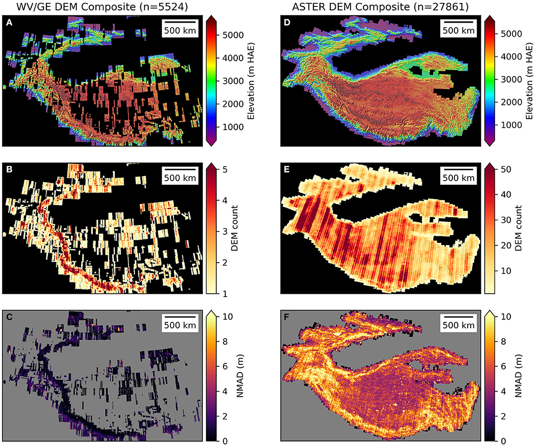
Figure 1. Composite products for WorldView/GeoEye (A–C) and ASTER (D–F) DEMs after co-registration and quality control. Rows show per-pixel weighted mean, count, and normalized median absolute deviation (NMAD). Note difference in color ramp for count maps in B and E.

2.2. ASTER DEMs

We generated DEMs from 28278 Level-1A (L1A) stereo images collected by the ASTER Visible and Near Infrared (VNIR) instrument (Fujisada, 1998) between June 2000 and June 2018 (Figure 1). We queried the NASA EarthData archive for daytime stereopairs (panchromatic bands 3N and 3B, 15 m GSD) with cloud cover <50%. The ASTER pairs were processed with ASP v2.6.0 using the void-filled SRTM-GL1 product as a seed DEM for initial orthorectification. We used the ASP semi-global matching (SGM) correlator (Hirschmuller, 2008) with default parameters (7 × 7 pixel window), which can offer improved results over the default ASP correlation routines for scenes with limited image resolution and/or texture (i.e., fresh snow-cover and cloud-shadowed areas). We used ASP's default SGM disparity map filters (3 × 3 pixel median filter and a 3 × 3 pixel “texture-aware smoothing filter” with scaling factor 0.13) to remove residual artifacts. Finally, isolated clusters of <50 pixels surrounded by missing data (“islands”) were removed from the disparity map. We used the rational polynomial coefficient (RPC) model bundled with each L1A scene for stereo triangulation, and culled outliers with large triangulation error (exceeding 3 × 75th-percentile) from the resulting point cloud. Output DEMs were posted at 30 m with elevations relative to the WGS84 ellipsoid. Finally, we performed a 2-pixel erosion of the outer DEM boundaries to remove any residual edge artifacts and filtered the resulting DEMs using an absolute elevation difference filter, removing any DEM pixels with ±100 m offset relative to the void-filled SRTM-GL1. The ASTER DEMs contain more noise than the WorldView/GeoEye DEMs, so we chose a more conservative threshold to remove spurious DEM pixels (e.g., artifacts near cloud margins), while also preserving the elevation change signals of interest over glacier surfaces.

2.3. TanDEM-X Global DEM

We used the publicly available TanDEM-X 1-arcsec (90 m) global DEM as a reference basemap for the region (Rizzoli et al., 2017; Wessel et al., 2018). While relatively coarse, this product offers excellent horizontal and vertical (~3.5 m absolute and <2 m relative) accuracy. We used the auxiliary products bundled with each DEM tile to mask artifacts/errors observed over some of the relatively steep terrain in HMA, including the theoretical height error map (HEM ≤ 1.5 m), water mask (33 ≤ WAM ≤ 127), and consistency mask (COM ≠ {0,1,2}). Qualitative inspection of DEM tiles around the region suggest that these filters removed most spurious pixels. Further details and code for TanDEM-X processing is available in the tandemx repository (Shean, 2019). The resulting products were used as a reference DEM for co-registration.

2.4. DEM Processing

2.4.1. Co-registration

All individual 30-m ASTER and 8-m WV/GE DEMs were co-registered to remove any horizontal and vertical offsets relative to the filtered reference TanDEM-X DEM. We identified “static” control surfaces that we assume did not change between the DEM acquisition timestamp and the reference DEM acquisition timestamp (~2011–2014 for TanDEM-X products). Both input DEMs were clipped to a common intersection and resampled to 30 m via bicubic interpolation. Glacier surfaces were masked with the RGI v6.0 polygons (RGI Consortium, 2017), and outlier elevation difference values over remaining static surfaces were identified and removed. We then used an iterative implementation of the Nuth and Kääb (2011) method, with robust filtering and outlier removal. If the resulting translation exceeded a 200 m threshold or if more than 30 iterations were required, the DEM was not used for subsequent analysis. For all other DEMs, the resulting horizontal translation was applied to each DEM and the median vertical bias was removed. We did not apply any corrections to residual differences (e.g., 5th order polynomials used by Brun et al., 2017), to avoid introducing additional elevation error over glacier surfaces due to overfitting of limited static control surfaces with poor spatial distribution. The dem_align.py script in the demcoreg package (Shean et al., 2019) outlines the full co-registration workflow.

We then analyzed the full set of co-registered ASTER and WV/GE DEMs to identify and remove any remaining problematic and/or low-quality DEMs. We estimated population statistics for both DEM sources using metrics from all individual DEMs before and after co-registration (Figure 2). We used these statistics to identify outliers and removed hundreds of DEMs with anomalously high residual bias and spread (Figures 2B,D). The dem_align_post.ipynb notebook in the demcoreg package (Shean et al., 2019) outlines the full post-coregistration outlier removal workflow. Figure 2 shows statistics for the final set of co-registered and validated DEMs.

FIGURE 2

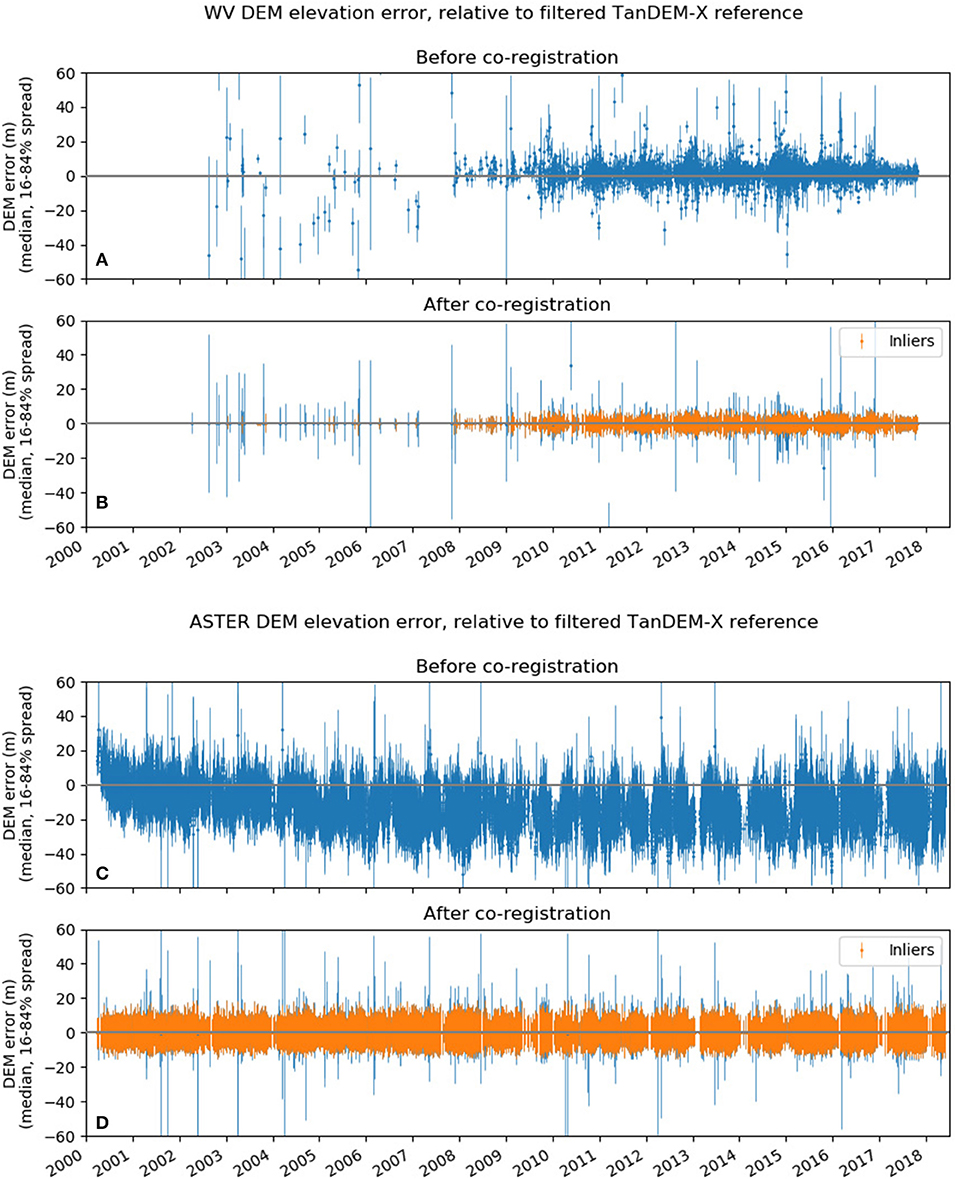
Figure 2. Temporal coverage and error metrics for WorldView/GeoEye (A,B) and ASTER (C,D) DEMs before and after co-registration. Each point shows the median elevation offset between an individual DEM and the TanDEM-X Global DEM reference over surfaces assumed to be static. Error bars show the 16–84% spread of these elevation offset values for each DEM. The final set of DEMs used for subsequent analysis and trend-fitting are shown with orange points/bars (“inliers”). Note the apparent drift in median offsets throughout the ASTER mission (C), and zero bias after co-registration.

2.4.2. Regional DEM Composites and Mosaics

We generated tiled DEM composite and mosaic products for the HMA region (Shean, 2017a) using the co-registered, filtered DEMs (Figure 1). All products use a custom Albers Equal Area projection that encompasses the RGI glacier polygons (PROJ4 string: +proj=aea +lat_1=25 +lat_2=47 +lat_0=36+lon _0=85 +x_0=0 +y_0=0 +ellps=WGS84 +datum = WGS84 +units=m +no_defs). We generated separate products for WV/GE and ASTER datasets, as well as a combined, blended, gap-free mosaic. Mosaic grid spacing was 8 m for WV/GE products and 30 m for ASTER products, with 100 × 100 km tiles. We also generated 1/3 arcsecond (~10 m) and 1-arcsecond (~30 m) resolution products using 1° × 1° tiles to conform with previous standards for global DEM mosaics (e.g., SRTM). The ASP dem_mosaic utility was used to generate seamless weighted-average composites and per-pixel composites of count, median, standard deviation, and normalized median absolute deviation (NMAD) using all valid DEM elevations at each pixel. We also generated timestamped mosaics using “forward” (most recent DEMs on top) and “reverse” (earliest DEM on top) per-pixel sort order, with associated products showing decimal year of elevation at each pixel. The code for composite and mosaic generation is available in the make_mos.sh and dem_mosaic_validtiles.py scripts in the gmbtools package (Shean and Bhushan, 2019).

2.4.3. Glacier DEM Stack Generation and Elevation Change Trend

We generated “stacks” of combined ASTER and WV/GE DEMs for each glacier polygon (plus a 1 km buffer) at 30 m posting. We computed linear elevation change trend ($\frac{dh}{dt}$, with units in m yr⁻¹) (Figure 3, Figure S1) for each pixel with >5 DEMs and >5 years between the first and last DEM timestamp. Several methods for the trend fitting were considered (Figure S1), including ordinary least-squares, random sample consensus (RANSAC), and the Theil-Sen estimator (scikit-learn implementation: https://scikit-learn.org/stable/modules/linear_model.html#theil-sen-regression). We reviewed maps of trend and residual values for a large sample of glaciers across the region, and confirmed that the robust Theil-Sen estimator offered superior output quality for the noisy ASTER+WV/GE DEM stacks (Figure S1).

FIGURE 3

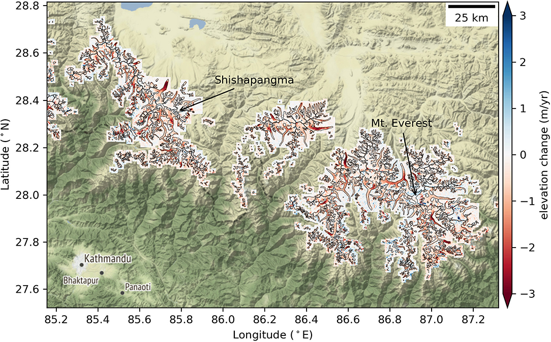
Figure 3. Annualized elevation change rate ($\frac{dh}{dt}$) for RGI glacier polygons (black outlines) from robust trend fits to stacks of ASTER+WV/GE DEMs for the period from 2000 to 2018.

The output elevation change trend map for each glacier was then filtered to remove artifacts. For each glacier (plus the buffered extent), a stack per-pixel median grid was created. From this grid, minimum (0.01 percentile) and maximum (99.99 percentile) stack elevation values were determined. These elevation values typically sampled the bottom of a valley floor, and the top of the highest peak in the scene. Then, these minimum and maximum elevation values were padded by and additional −150 and +150 m, respectively. Per-pixel elevation change trends were extrapolated to obtain surface elevation maps for May 31, 2000 and May 31, 2018. If the extrapolated elevations fell outside of the padded bounds, the pixel was masked. A 1-pixel erosion step removed trend values near data gaps, and a 3 × 3-pixel median filter followed by a 3 × 3-pixel Gaussian filter were used to remove residual outliers and smooth the output trend maps (Figure 3). Details of this workflow can be found in the stack_interp.py script in the gmbtools package (Shean and Bhushan, 2019).

2.5. Glacier Mass Balance

We computed glacier mass balance and mass balance uncertainty at multiple spatial scales: individual glacier polygons, tessellated hexagonal grid cells, glacierized regions, river basins, and the full HMA domain. We use $\frac{d}{dt}$ notation for pixel values, and Δ notation for spatially aggregated values, with both representing the annualized rate of change for the period from 2000 to 2018.

2.5.1. Individual Glacier Mass Balance

We used the elevation trend maps to estimate geodetic mass balance for glacier polygons with a minimum of 85% coverage. In practice, 95% of the glaciers in the study area had >97% coverage, eliminating the need to rely on gap-filling approaches (e.g., McNabb et al., 2019). We computed $\frac{dh}{dt}$ statistics for each glacier polygon, computed mean glacier elevation change Δh, and multiplied by polygon area A to estimate total individual glacier volume change ΔV. We used a standard bulk density estimate ρ = 850 kg m⁻³ (Huss, 2013) to convert this volume change to individual glacier total mass balance ΔM:

$\begin{array}{ll}\Delta M=\Delta h·A·\rho & (1)\end{array}$

In contrast to many previous studies, we did not impose a minimum glacier area threshold, and consider all 95536 HMA glacier polygons in RGI v6.0.

2.5.2. Individual Glacier Mass Balance Uncertainty

We calculated individual glacier mass balance uncertainty using approaches similar to those outlined in recent geodetic analyses with similar DEM sources (e.g., Fischer et al., 2015; Berthier et al., 2016; Brun et al., 2017; Menounos et al., 2019).

To estimate glacier elevation change error σ_Δh, we calculated statistics for per-pixel $\frac{dh}{dt}$ trend values within a 500 m buffer around each glacier polygon, assuming $\frac{dh}{dt}$ values should be 0 for these “static” or “stable” surfaces. We then combined “random” and “systematic” error components to estimate total error.

To estimate random error ${{\sigma }_{\frac{dh}{dt}}}_{random}$ (i.e., spread of $\frac{dh}{dt}$ noise), we considered both the NMAD and standard deviation of $\frac{dh}{dt}$ values over static surfaces. We used the Rolstad et al. (2009) “rule of thumb” approach, and a decorrelation length scale L of 500 m between pixels in the $\frac{dh}{dt}$ maps. We scaled the ${{\sigma }_{\frac{dh}{dt}}}_{random}$ values for glaciers with A ≥ πL² (~0.78 km²) by an area-dependent coefficient $\sqrt{\frac{\pi L^2}{5A}}$ (Rolstad et al., 2009), which accounts for the fact that larger areas dominated by uncorrelated random error will approach 0 mean error. To account for any residual systematic error ${{\sigma }_{\frac{dh}{dt}}}_{systematic}$ (i.e., local $\frac{dh}{dt}$ bias), we computed the mean of $\frac{dh}{dt}$ values over the same static surfaces. We then combined this ${{\sigma }_{\frac{dh}{dt}}}_{systematic}$ value with the scaled ${{\sigma }_{\frac{dh}{dt}}}_{random}$ value (computed from the standard deviation of $\frac{dh}{dt}$ values) in quadrature to estimate total root-mean-square error (RMSE):

$\begin{array}{ll}{\sigma }_{\Delta h}=\sqrt{{{{\sigma }_{\frac{dh}{dt}}}_{random}}^2+{{{\sigma }_{\frac{dh}{dt}}}_{systematic}}^2}& (2)\end{array}$

Many previous studies report σ_Δh as the scaled ${{\sigma }_{\frac{dh}{dt}}}_{random}$ component from the NMAD of $\frac{dh}{dt}$ values. These NMAD-only error estimates are more robust to outliers and tend to be relatively small. The combined RMSE estimates from Equation (2) are larger and more conservative, and we use these values for σ_Δh in this study.

Though the reported RGI inventory uncertainty is ~8% for HMA (Pfeffer et al., 2014), we assumed glacier polygon area uncertainty of 10% (σ_A = 0.1·A) (e.g., Kääb et al., 2012) to account for any polygon digitization error, temporal evolution of glacier extent during the study period [e.g., changes related to retreat, surging, and other ice dynamics (e.g., Azam et al., 2018)], and offsets between the source image timestamps used for RGI polygon digitization (~1998–2014) and the DEM timestamps. We assumed density uncertainty σ_ρ = 60 kg m⁻³ (Huss, 2013), which is 7.1% of ρ = 850 kg m⁻³.

Assuming that the three error components (σ_Δh, σ_A, σ_ρ) are independent and uncorrelated, the total mass change uncertainty for each glacier polygon is:

$\begin{array}{ll}{\sigma }_{\Delta M}=\sqrt{{(A·\rho ·{\sigma }_{\Delta h})}^2+{(\Delta h·\rho ·{\sigma }_A)}^2+{(\Delta h·A·{\sigma }_{\rho })}^2}& (3)\end{array}$

(using Equation 10 in Joint Committee for Guides in Metrology, 2008). An alternative form of this equation can be written in terms of normalized, dimensionless fractional uncertainty:

$\begin{array}{ll}{\sigma }_{\Delta M}=|\Delta M|·\sqrt{{\left(\frac{{\sigma }_{\Delta h}}{\Delta h}\right)}^2+{\left(\frac{{\sigma }_A}{A}\right)}^2+{\left(\frac{{\sigma }_{\rho }}{\rho }\right)}^2}& (4)\end{array}$

which is convenient given that our area and density uncertainty are provided as percentages. While Equation (4) appears to be undefined for |Δh| = 0, if we distribute the |ΔM| term, then as $|\Delta h|\to 0,{\sigma }_{\Delta M}\to \sqrt{{(A·\rho ·{\sigma }_{\Delta h})}^2}$. The mb_parallel.py script in the gmbtools package (Shean and Bhushan, 2019) contains the detailed workflow used for individual glacier mass balance and uncertainty estimation.

As defined above, we assume $\frac{{\sigma }_A}{A}=0.10$ and $\frac{{\sigma }_{\rho }}{\rho }=0.071$, so the minimum glacier mass balance uncertainty will be ~12.2% when $\frac{{\sigma }_{\Delta h}}{|\Delta h|}$ is 0. In practice, the $\frac{{\sigma }_{\Delta h}}{|\Delta h|}$ term tends to dominate the mass balance uncertainty for individual glaciers, but aggregation over larger areas reduces its influence on total mass balance uncertainty.

2.5.3. Aggregated Glacier Mass Balance

We aggregated the individual glacier mass balance results for the full HMA region and different sub-regions. We computed centroids for each glacier polygon and performed spatial joins to compile statistics for the centroids that fell within larger sub-region polygons. The sub-region aggregation was performed for the commonly used glacierized regions of Kääb et al. (2015) and the HIMAP project (Bolch et al., 2019), the major hydrologic basins (Vörösmarty et al. (2010), updated to 6-min spatial resolution), and the Goddard GRACE mascon boundaries (Loomis et al., 2019). We modified three of the Kääb et al. (2015) regions to remove references to country names (“Bhutan” → “East Himalaya,” “East Nepal” → “Central Himalaya” and “West Nepal” → “West Himalaya”).

For each sub-region, we computed the sum of glacier mass balance (ΔM) for all n_glac glaciers in cubic meters water equivalent (m³ w.e. yr⁻¹) and gigatons per year (Gt yr⁻¹) and divided by aggregated glacier area to obtain mean specific mass balance (m w.e. yr⁻¹). We converted Gt to mm sea level rise equivalent using a global ocean area estimate of 3.625 × 10⁸ km² (Cogley et al., 2011), and considered total contributions from all glaciers and then only those glaciers within exorheic basins.

2.5.4. Aggregated Glacier Mass Balance Uncertainty

Estimating total mass balance uncertainty for larger aggregation areas is more complex than for individual glaciers. Many previous studies compute Δh for all valid $\frac{dh}{dt}$ pixels over glaciers and σ_Δh for all $\frac{dh}{dt}$ pixels over stable surfaces in the area of interest (e.g., river basin, 1° × 1° cells), often aggregating statistics for elevation bins and scaling using observed glacier hypsometry. The uncertainty is sometimes scaled to account for relatively short autocorrelation length scales of $\frac{dh}{dt}$ pixel values over stable areas (e.g., ~500 m), but rarely for longer autocorrelation length scales (e.g., 10s of km). It is also possible that glacier polygons could be split across aggregation boundaries (e.g., glacier accumulation area in one 1° × 1° cell and ablation area in adjacent cell), which will bias aggregated mass balance estimates.

To avoid these issues, we aggregated mass balance uncertainty values for individual glacier polygons, not $\frac{dh}{dt}$ pixels. Initially, we used the individual glacier mass balance uncertainty values (σ_ΔM) from Equation (3). Combining these values in quadrature resulted in unrealistically low aggregated uncertainty estimates for the full-HMA region (0.3 Gt yr⁻¹ or 1.7%) due to the large glacier sample size (n_glac ≈ 95,000 for full-HMA region). This approach assumes that the σ_ΔM values for all glacier polygons are independent and completely uncorrelated, which is incorrect for several reasons: the density uncertainty σ_ρ is constant for all glaciers (perfect spatial autocorrelation), area uncertainty percentage $\frac{{\sigma }_A}{A}$ is also constant for all glaciers, and there is inevitably some large-scale (~10s of km) spatial autocorrelation of $\frac{dh}{dt}$ pixel values over stable terrain that is not accounted for using the scaling described in section 2.5.2. This large-scale σ_Δh spatial autocorrelation is controlled by the input DEM sample counts (Figure 1), DEM dimensions (~ 60 × 60 km for ASTER), DEM artifact length scales, and slope- and aspect-dependent residual co-registration errors.

If we instead assume that the σ_ΔM values are perfectly correlated and compute the sum of all σ_ΔM during aggregation, we obtain unrealistically high aggregated uncertainty estimates for the full-HMA region (21.5 Gt yr⁻¹ or 113.4%). A more appropriate estimate of aggregated mass balance uncertainty falls between these two approaches, as the errors are correlated, but only over a limited range of length scales (e.g., Rolstad et al., 2009; Anderson, 2019). To estimate these length scales, we calculated the range of autocorrelation for σ_ΔM values using experimental semivariograms with a lag distance equal to the median of the nearest neighbor distances between glacier polygon centroids (~786 m). We fit a spherical semivariogram to the experimental semivariogram using ordinary least squares, and obtained an autocorrelation length scale estimate of ~42 km for σ_ΔM using the RMSE error metric (Equation 2) and ~27 km for σ_ΔM using the NMAD error metric. See Figure S2 for details and the Mass_balance_cor_working.ipynb notebook in the raster_geostatistics repository (Bhushan, 2020) for additional details.

This approach using total mass balance uncertainty for each glacier (σ_ΔM), however, fails to consider variable spatial autocorrelation length scales for the individual components of σ_ΔM in Equation (4). A better strategy is to isolate and consider the spatial autocorrelation of only the σ_Δh values, as the σ_ρ and $\frac{{\sigma }_A}{A}$ values are constant across the region, and their inclusion will increase apparent spatial autocorrelation of the σ_ΔM values. We repeated our semivariogram analysis for the σ_Δh values and found an autocorrelation length scale of ~32 km for the σ_Δh RMSE and ~24 km for the σ_Δh NMAD error metrics (Figure S2) (dh_dt_sigma_error.ipynb in Bhushan, 2020).

Based on the range of influence for the σ_Δh RMSE values, we defined a tessellated grid of hexagonal cells across the HMA domain to represent independent spatial samples with “radius” of 32 km. The width between opposite sides of these hexagon cells is 55 km, which is roughly equivalent to a quarter-degree cell. We note that aggregation for cells defined in units of decimal degrees (e.g., 1° × 1° cells used by many previous HMA-wide inventories) can be problematic, as the cells cover variable total area at different latitudes. For example, a 1° × 1° cell at 25°N covers ~11,182 km² while a 1° × 1° cell at 47°N covers ~8,455 km², an areal difference of ~24%. To avoid potential sampling bias, we defined these equal-area hex cells in our custom equal-area projection (section 2.4.2).

We computed the mean glacier elevation change for each hex cell (Δh_cell) using the sum of all individual glacier volume change (ΔV = Δh·A) estimates for the n_glac glacier polygon centroids that fell within each cell:

$\begin{array}{ll}{\Delta h}_{cell}=\frac{{\displaystyle {\sum }_{i=1}^{n_{glac}}}{\Delta h}_i·A_i}{A_{cell}}& (5)\end{array}$

where A_cell is the total area of the n_glac glacier polygons in the cell. Mean sample size (n_glac) for the 55-km hex cells was 119, with a range of 1–585 (Figure S3). We substituted Δh_cell and A_cell into Equation 1 to compute cell-level total mass balance ΔM_cell.

To estimate hex cell elevation change uncertainty (σ_Δhcell), we computed the sum of all individual glacier volume uncertainty (σ_ΔV = σ_Δh·A) estimates for the n_glac glacier polygon centroids that fell within each hex cell, assuming they were correlated (based on the semivariogram analysis above):

$\begin{array}{ll}{\sigma }_{{\Delta h}_{cell}}=\frac{{\displaystyle {\sum }_{i=1}^{n_{glac}}}{\sigma }_{{\Delta h}_i}·A_i}{A_{cell}}& (6)\end{array}$

With this approach, we effectively weight the σ_Δh estimate for each glacier by the relative glacier area $\frac{A}{A_{cell}}$. While the area terms in Equation (6) also have some uncertainty, the common 10% relative area uncertainty will cancel, so it does not directly contribute to the σ_Δhcell estimate. We used Equation (4) to compute total mass balance uncertainty for the cell (σ_ΔMcell), which accounts for this area uncertainty.

For subsequent aggregation over larger HMA sub-regions, we computed mean glacier elevation change (Δh_agg) as the sum of all hex cell glacier volume change (ΔV_cell = Δh_cell·A_cell) estimates for the n_cell hex cell centroids that fell within each aggregation polygon containing total glacier area A_agg:

$\begin{array}{ll}{\Delta h}_{agg}=\frac{{\displaystyle {\sum }_{i=1}^{n_{cell}}}{{\Delta h}_{cell}}_i·{A_{cell}}_i}{A_{agg}}& (7)\end{array}$

which is similar to Equation (5). We assumed that σ_Δhcell errors for adjacent hex cells were independent and uncorrelated, and computed aggregated elevation change uncertainty (σ_Δhagg) in quadrature for all n_cell hex cells that fell within each aggregation polygon:

$\begin{array}{ll}{\sigma }_{{\Delta h}_{agg}}=\frac{\sqrt{{\displaystyle {\sum }_{i=1}^{n_{cell}}}{({\sigma }_{{{\Delta h}_{cell}}_i}·{A_{cell}}_i)}^2}}{A_{agg}}& (8)\end{array}$

Sample sizes for this aggregation (n_cell) were 7–79 for HIMAP regions, 22–327 for Kääb et al. (2015) regions, and 3–117 for hydrologic basins, with a total of 793 hex cells for the full-HMA region. We used these values and Equations (1) and (4) to compute total mass balance ΔM_agg and uncertainty σ_ΔMagg for the aggregated regions.

To summarize, we estimated uncertainty for each glacier using observed $\frac{dh}{dt}$ values on surrounding terrain. We aggregated glacier mass balance and uncertainty values for spatially correlated hex cell samples, then aggregated these independent samples in quadrature for regional and full-HMA uncertainty estimates.

2.6. Glacier Meltwater Runoff

While we cannot directly estimate total glacier meltwater runoff contributions from glacierized HMA river basins using our geodetic mass balance estimates, we can estimate the “excess meltwater runoff” (e.g., Radić and Hock, 2014; Brun et al., 2017) or “imbalance component of runoff” (e.g., Pritchard, 2019). This excess glacier meltwater runoff is equal to the glacier mass loss in a given basin (Brun et al., 2017; Pritchard, 2019; Rounce et al., 2020b). In this study, we compute mass loss at multiple scales (individual glaciers, hex cells, basins), and we report excess glacier meltwater runoff for a given basin as the water-equivalent loss from only the glaciers or hex cells with negative mass balance (ΔM < 0) in that basin. The total excess glacier meltwater runoff can therefore be larger than the total glacier mass loss for the basin, as any glaciers or hex cells with positive mass balance are not included. To avoid thresholding issues (e.g., Anderson, 2019), we conservatively estimate excess glacier meltwater runoff uncertainty as the aggregated total glacier mass balance uncertainty for each basin.

To assess the relative importance of this excess glacier meltwater runoff, we compared with existing model output for the “total glacier meltwater runoff” and “total runoff” in each basin, which provided estimates for excess meltwater “percent of total glacier meltwater runoff” and “percent of total runoff.”

The total glacier meltwater runoff was estimated from Python Glacier Evolution Model (PyGEM, https://github.com/drounce/PyGEM), forced with ERA-Interim reanalysis data (Rounce et al., 2020a,b). The monthly meltwater runoff was modeled for a single “gauging station” that moves with the terminus of each glacier and is the sum of modeled balance runoff expected if all glaciers were in equilibrium and any excess (or imbalance) runoff due to mass loss. The monthly values were annualized, and the 2000 to 2018 mean annual total glacier meltwater runoff was computed for each HMA basin, with final values of ~0.1 to 25 Gt yr⁻¹ (Rounce et al., 2020a,b).

The total runoff for each basin includes all water that moved from the land surface to the river system, including total glacier meltwater runoff, surface runoff (precipitation, snow melt), and groundwater baseflow. We used output from the Water Balance Model (WBM) (Wisser et al., 2010) forced with 1980–2016 ERA-Interim reanalysis data (Grogan, 2016) to estimate mean annual total runoff (at basin mouth for exorheic basins, and total area runoff for endorheic basins) during the 2000–2016 period (D. Grogan, personal communication). These basin-specific values ranged from ~12 to 1,094 Gt yr⁻¹, and they show good agreement with available gauge observations (GRDC, 2018) and model output (Huss and Hock, 2018).

3. Results

3.1. Glacier Mass Balance

The total HMA glacier mass balance for the period from 2000 to 2018 was −19.0 ± 2.5 Gt yr⁻¹ (−0.19 ± 0.03 m w.e. yr⁻¹). Maps of aggregated values for hex grid cells show the detailed spatial distribution of glacier mass change across the full HMA region (Figure 4, Figure S4). The Himalayan range displays relatively large mass loss, with some spatial variability. Clusters of grid cells with more positive mass balance are observed in the Kunlun and Karakoram ranges. The mass balance gradient across the Karakoram (slightly positive/near-balance in the west, slightly negative in the east) is consistent with results from recent analyses (Lin et al., 2017; Berthier and Brun, 2019). Hex cell uncertainty values are highest in the Nyainqentanglha and Eastern Tien Shan, where total DEM counts are lowest (Figure 1E) and individual glacier uncertainty is high.

FIGURE 4

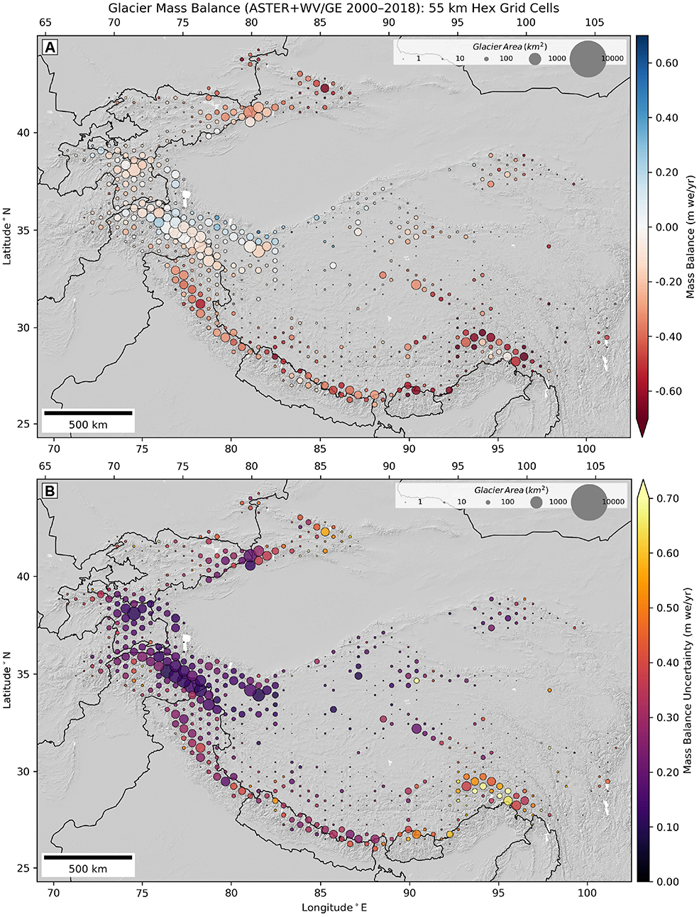
Figure 4. (A) Specific glacier mass balance (m w.e. yr⁻¹) and (B) uncertainty for the period from 2000 to 2018, aggregated over 55 km hex grid cells. The size of the circle for each cell is scaled by total glacierized area within that cell. Approximate international borders from Natural Earth 1:10M products are plotted for reference. See Figure S4 for units of Gt yr⁻¹.

Regional aggregations show greatest specific mass loss rates (Figure 5) and total mass loss rates (Figure S5) across Western, Central, and Eastern Himalayas, Nyainqentanglha, and the Central and Eastern Tien Shan. The Western Kunlun Shan and Eastern Pamir showed slightly positive mass balance, while the Karakoram showed slightly negative mass balance. Our results suggest that the HiMAP sub-region aggregation offers better spatial resolution of mass change patterns than the Kääb et al. (2015) sub-regions. This is especially true for the Tien Shan and Inner Tibetan Plateau, with more negative specific mass balance is observed in the eastern HiMAP sub-regions, though total mass loss for these sub-regions is relatively small (Figure S5).

FIGURE 5

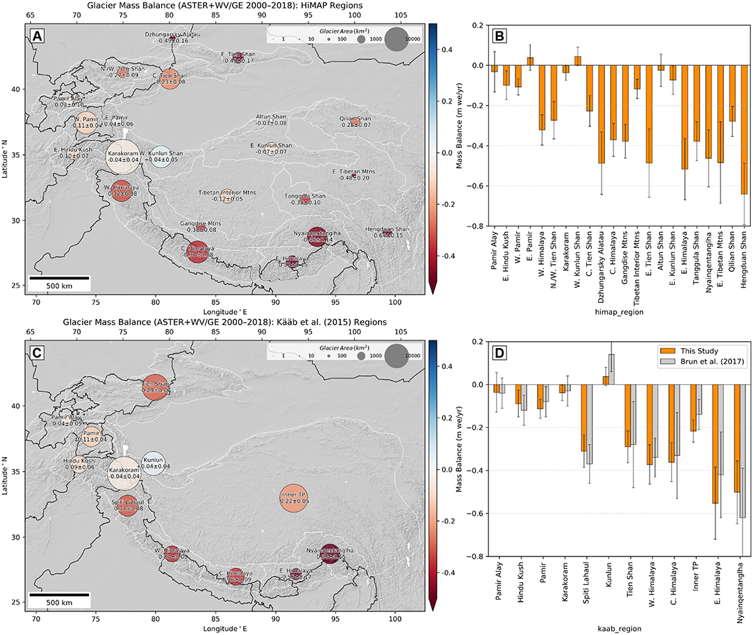
Figure 5. Specific glacier mass balance (m w.e. yr⁻¹) for the period from 2000 to 2018, aggregated over glacierized sub-regions from (A,B) HiMAP (Bolch et al., 2019) and (C,D) Kääb et al. (2015). Circle color shows mass balance and circle size is scaled by total glacier area for each sub-region (white outlines). Bar plots are sorted by x-coordinate of the sub-region polygon centroid. Updated values (Brun et al., 2018) from Brun et al. (2017) are plotted in (D) for comparison. See Figure S5 for units of Gt yr⁻¹.

3.2. Mass Balance and Glacier Area

Our results show that larger glaciers dominate total HMA mass balance (Figure 6). In terms of specific mass balance (m w.e. yr⁻¹), we found that glaciers between ~0.1 and ~10 km² clustered around the mean specific mass balance for the full dataset (Figure 6A). Glaciers smaller than ~0.1 km² had more positive specific mass balance relative to the mean, while glaciers between ~10 and ~30 km² were more negative (Figure 6A). Glaciers larger than ~100 km² are concentrated in western HMA (Figure 6C), where more positive mass balance was observed during the period from 2000 to 2018. This indicates that the limited sample of very large glaciers is not necessarily representative of glacier change across the full HMA domain.

FIGURE 6

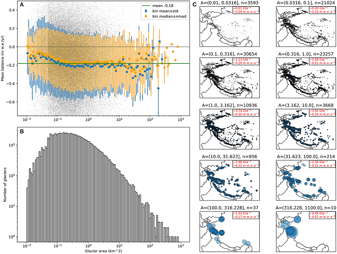
Figure 6. (A) Relationship between specific glacier mass balance and glacier area. (B) Histogram of glacier area. (C) Spatial distribution of glaciers in each area bin, represented as circles scaled by glacier area. The largest circle in the lower right plot covers 1077 km². Subplot titles include area bin bounds in km² (e.g., “A = [0.01, 0.316]”) and number of glaciers in the bin (e.g., “n = 3593”). Annotation in upper right corner shows total mass balance and mean specific mass balance for all glaciers in the bin.

3.3. River Basins and Meltwater Runoff

All glacierized HMA river basins had negative glacier mass balance for the period from 2000 to 2018 (Figure S6). Glacier mass balance for exorheic and endorheic basins was −13.28 ± 2.28 Gt yr⁻¹ and −5.69 ± 1.49 Gt yr⁻¹, respectively. The Brahmaputra had greatest total glacier mass loss (−4.87 ± 1.01 Gt yr⁻¹), followed by the Indus (−3.53 ± 0.97 Gt yr⁻¹) and Ganges (−3.19 ± 0.58 Gt yr⁻¹).

Total HMA-wide excess glacier meltwater was −22.71 ± 3.01 Gt yr⁻¹ when calculated using all individual glaciers with negative mass balance, −20.61 ± 2.73 Gt yr⁻¹ when calculated using all hex cells with negative mass balance, and −19.0 ± 2.5 Gt yr⁻¹ when calculated using all aggregated basins with negative mass balance (identical to total mass balance, as all basins are negative). These differences emphasize the importance of aggregration level and methodology for this calculation. The Brahmaputra, Indus, and Ganges river basins had the greatest total excess glacier meltwater runoff, with glaciers contributing 5.23 (4.87) Gt yr⁻¹, 4.55 (3.92) Gt yr⁻¹, and 3.26 (3.19) Gt yr⁻¹ above balance glacier meltwater runoff to their respective river systems during the 2000 to 2018 period (Figure 7A) for all glaciers (hex cells).

FIGURE 7

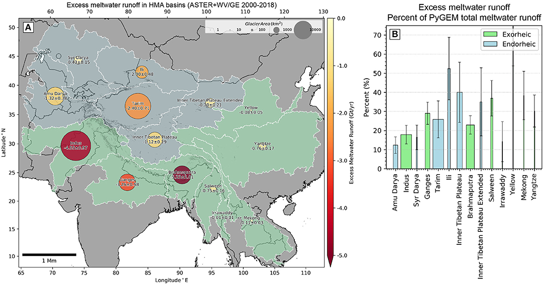
Figure 7. Excess glacier meltwater runoff between 2000 and 2018 for major river basins in HMA: (A) Spatial distribution (Gt yr⁻¹), and (B) as a percentage of mean annual PyGEM model total (combined balance and imbalance) glacier meltwater runoff (Rounce et al., 2020a,b). To highlight excess glacier meltwater runoff contributions for highly glacierized basins, bar width is scaled by the percent glacierized area in each basin (total glacier area divided by basin area, with values of ~0.0–2.1%). Error bars combine basin-specific excess glacier meltwater uncertainty and interannual variability of modeled total glacier meltwater runoff for the 2000–2018 period. The Irrawady, Yellow, and Mekong basins have negligible glacierized area (~30–200 km²) and are sensitive to basin definitions and aggregation strategy, resulting in less-reliable percentages.

The basin-specific excess glacier meltwater runoff percentage of total glacier meltwater runoff ranged from ~12 to 53%, with values of ~25–53% observed for the interior, endorheic basins of the western Tibetan Plateau (Tarim, Ili, Inner Tibetan Plateau), and values of ~18-29% observed for highly glacierized, exorheic basins (Indus, Ganges, Brahmaputra) (Figure 7B). The basin-specific excess glacier meltwater runoff percentage relative to total basin runoff (including precipitation, snow melt, base flow) ranged from ~0.0–3.3%, with relatively high values (~1.7–3.3%) for interior, endorheic basins (Tarim, Ili, Inner Tibetan Plateau Extended), ~1.5% for the Indus, and ~0.6% for the Ganges and Brahmaputra.

3.4. Sea Level Rise Contribution

The total potential sea level rise contribution from HMA glacier mass loss between 2000 and 2018 was up to 0.052 ± 0.007 mm SLE yr⁻¹ (19.0 ± 2.5 Gt yr⁻¹). The contribution from exorheic basins was 0.037 ± 0.006 mm SLE yr⁻¹ (13.3 ± 2.3 Gt yr⁻¹).

This HMA contribution was ~4-6% of the 0.92± 0.39 mm SLE yr⁻¹ total contribution from all global glaciers and ice caps for this period (Zemp et al., 2019), and a small but non-negligible fraction (~1.0-1.5%) of total global sea level rise estimates of 3.5 ± 0.2 mm SLE yr⁻¹ from 2005-2018 (WCRP Global Sea Level Budget Group, 2018). The total cumulative sea level contribution of HMA glaciers for the period from 2000 to 2018 was up to 0.94 ± 0.13 mm SLE, with 0.65 ± 0.11 mm SLE from exorheic basins.

4. Discussion

4.1. Glacier Mass Balance Methodology

The nearly complete inventory (99% of RGI polygons) of glacier mass balance provides an important snapshot of the detailed spatial pattern of glacier change across the region. We considered all glaciers in HMA (without a minimum area threshold), aggregated these glaciers into independent samples based on observed autocorrelation length scales, and then aggregated these independent samples over larger regions for improved uncertainty estimates. This approach offered a systematic regional assessment, with better coverage over sub-regions containing relatively small and/or sparse glaciers (e.g., eastern Tibetan Plateau) that could not be measured or were excluded from previous assessments.

A common issue with geodetic glacier mass balance studies is missing data over portions of glacier polygons, especially accumulation areas. These data gaps can be filled using several methods (McNabb et al., 2019), which can lead to significant differences in estimates for glacier mass balance and uncertainty. Our study involves the most complete coverage for HMA glaciers to date, with mean polygon coverage of 99.5% and <5% missing data for 98% of all RGI glacier polygons, precluding the need for more complex gap-filling approaches.

4.2. Glacier Mass Balance Uncertainty

Our results underscore the importance of aggregation methodology for mass balance uncertainty calculations. Individual glacier mass balance uncertainty estimates can be large, often exceeding the magnitude of the apparent change, especially for smaller glaciers. Aggregation significantly reduces the combined mass balance uncertainty, though final estimates can vary greatly depending on methodology.

Unlike many other studies (Rolstad et al., 2009; Nuth and Kääb, 2011; Brun et al., 2017), we did not fit higher-order, 2-D polynomials to $\frac{dh}{dt}$ residuals and remove from static surfaces after co-registration. While doing so would significantly reduce apparent ${{\sigma }_{\frac{dh}{dt}}}_{systematic}$ bias and large-scale spatial autocorrelation, it would inevitably overfit sparse $\frac{dh}{dt}$ samples in many areas and adversely impact glacier mass balance estimates.

We found that large-scale autocorrelation length scales varied depending on the choice of error metric (section 2.5.2), with ~24 km for σ_Δh from NMAD, ~32 km for σ_Δh from RMSE, ~27 km for σ_ΔM from NMAD, and ~42 km for σ_ΔM from RMSE (Figure S2). The increased range of influence for the RMSE metrics is likely related to spatially coherent residual $\frac{dh}{dt}$ bias over static surfaces. In addition, we found that the apparent autocorrelation length scales (range of influence) was sensitive to the step and total lag distance used during semivariogram analysis. Finally, we found that common assumptions about circular, isotropic range of influence are likely an oversimplification, as we observe different autocorrelation length scales for directional semivariogram analysis (dh_dt_sigma_error.ipynb in Bhushan, 2020).

Our hex cell approach attempts to account for spatial autocorrelation of σ_Δh error between individual glacier polygon centroids. This is potentially an oversimplification. For one, adjacent polygons may share the same “stable” ground (e.g., ridge between two valley glaciers), resulting in greater apparent spatial autocorrelation than would be found with a regional analysis of ${{\sigma }_{\frac{dh}{dt}}}_{random}$. In addition, rather than the geometric centroid of 2-D glacier polygons, it would be better to use the 3-D “center of mass” for each glacier from gridded ice thickness products (e.g., Huss and Farinotti, 2012), especially when aggregating over GRACE mascons. While this approach will not affect smaller glaciers, it could better represent longer glaciers with curved centerlines.

The hex cell and sub-region aggregation mass balance uncertainty is sensitive to the hex cell size, though full-HMA mass balance values are not affected. We experimented with several hex cell widths (27–55 km) and multiple offsets for the hex cell grid origin. Due to assumptions about spatial dependence (Equation 6), the individual hex cell uncertainty values increase with greater cell area, as do the corresponding uncertainty values for regional aggregation. A related issue involves width-dependent hex cell centroid locations and partitioning amongst different regional aggregation polygons (e.g., adjacent river basins). In practice, we did not observe significant differences in aggregated mass balance values for the range of hex cell widths tested.

Instead of an intermediate hex cell aggregation based on spatial autocorrelation of σ_Δh values assigned to glacier centroids, one could explore a nested spherical semivariogram model (Rolstad et al., 2009) to simultaneously account for small-scale (~500 m) and large-scale (~20–30 km) autocorrelation of $\frac{dh}{dt}$ values over arbitrary aggregation areas. This nested approach would require a relatively large sample of well-distributed $\frac{dh}{dt}$ values over stable surfaces to properly capture the large-scale variability. There are also potential issues with this approach for complex (i.e., non-circular) aggregation polygon geometry (e.g., elongated mountain ranges) and observed anisotropy in spatial autocorrelation.

Our ~10% glacier polygon area uncertainty assumption is likely overestimating actual uncertainty for the RGI v6.0 inventory, especially when aggregated over the entire region. While inventory error is difficult to assess, the study by Pfeffer et al. (2014) estimated area uncertainty of ~8% for HMA and ~5% for all glacier regions in the RGI v3.2 inventory. While an individual glacier may have area uncertainty of 10% or more (e.g., a relatively small, surging glacier), it is unlikely that all glaciers in aggregated regions have area uncertainty of 10%. For larger aggregation areas, the area uncertainty term dominates the total mass balance uncertainty in Equation (4), which justifies future efforts to improve time-variable inventories of glacier outlines.

We are hopeful that future community-driven, open-source software development will continue to standardize these methods, enabling more systematic glacier mass balance and uncertainty estimates for HMA and other glacierized regions.

4.3. Comparison With Previous Work

Our results are generally consistent with other full-HMA glacier mass balance assessments, including the comprehensive review by Bolch et al. (2019) and recent analysis by Brun et al. (2017). Considering the range of methods, datasets, time periods and spatial coverage of previous studies, we limit our direct comparison with the “reference” analysis by Brun et al. (2017) (similar methods, similar time period), and refer the reader to Brun et al. (2017) for detailed comparisons with earlier work, and to Bolch et al. (2019) for more complete context.

4.3.1. Full HMA Glacier Mass Balance

Our total HMA-wide mass balance of −19.0 ± 2.5 Gt yr⁻¹ (−0.19 ± 0.03 m w.e. yr⁻¹) is larger than the −16.3 ± 3.5 Gt yr⁻¹ (−0.18 ± 0.04 m w.e. yr⁻¹) estimate by Brun et al. (2017), although the two are within uncertainty bounds. While this difference in total mass loss rate may be related to differences in methodology, it could also be influenced by the inclusion of an additional 2+ years (2016–2018) of DEMs later in the 2000 to 2018 study period. Based on observed long-term glacier mass balance trends for HMA (e.g., Mukherjee et al., 2018; Zhou et al., 2018; Maurer et al., 2019) and glaciers worldwide, we might expect greater mass loss toward the end of the record as opposed to earlier in the record. Despite a more negative total mass balance, we find a smaller sea level rise contribution from exhoreic basins (13.3 ± 2.3 Gt yr⁻¹) compared to the 14.6 ± 3.1 Gt yr⁻¹ estimate by Brun et al. (2017).

4.3.2. Sub-region Glacier Mass Balance

We used the recently published HiMAP sub-region definitions (Bolch et al., 2019) during aggregation, which provide improved geographic partitioning of mass balance for HMA mountain ranges, especially over the Inner Tibetan Plateau and Tien Shan. However, most existing full-HMA geodetic mass balance assessments are limited to the sub-regions defined by Kääb et al. (2015). We generally observe good agreement between our results and those of Brun et al. (2017) for the Kääb et al. (2015) sub-region definitions (Figure 5D, Figure S5D). The most notable differences for total mass balance in Gt yr⁻¹ (Figure S5D) are over the Kunlun, where our mass gain estimates are smaller, and the Inner Tibetan Plateau where our mass loss estimates are larger. Larger differences in specific mass balance (Figure 5D) are observed for the Eastern Himalaya and Nyainqentanglha. These differences potentially arise from relatively limited observations for these sub-regions in the study by Brun et al. (2017).

4.3.3. River Basins and Meltwater Runoff

Our estimates for total mass balance in HMA river basins are generally similar to those by Brun et al. (2017) (Figure S6), with notable differences for the Tarim and Inner Tibetan Plateau (Figure S6D). In both cases, our mass loss estimates are larger than those of Brun et al. (2017), with an apparent sign change for Tarim (−0.87± 0.71 Gt yr⁻¹ in our study vs. +0.4± 1.3 Gt yr⁻¹ in Brun et al., 2017), which is important for full HMA excess glacier meltwater estimates. Some of this discrepancy may be related to basin boundary definitions, but our estimates are consistent with observed differences in glacierized sub-region mass balance estimates over the Kunlun and Tien Shan (Figure S5).

While the total mass balance estimates are important for assessing HMA contributions to sea level rise, the excess glacier meltwater runoff potentially provides information on the long-term mean of seasonal glacier contributions to downstream hydrology. The largest differences between the two metrics are observed for basins with a relatively high percentage of glaciers with positive mass balance (e.g., Indus, Tarim). Our estimates for total excess glacier meltwater runoff are generally similar to those provided by Brun et al. (2017). We note that estimates for excess glacier meltwater runoff vary based on aggregation methodology, with more negative values obtained when aggregating at the glacier polygon level compared with the hex cell or basin level (used by Brun et al., 2017).

To provide context for our observed excess glacier meltwater runoff estimates, we considered the percentage of modeled total glacier meltwater runoff and total runoff in each basin. While these estimates vary based on glacier/hydrologic model, forcing data, and true interannual variability, the long-term mean runoff (2000–2016) should capture the relative magnitudes across HMA basins. Our results show that a significant portion of large, endorheic basins on the Tibetan Plateau contain relatively high percentages of excess glacier meltwater (Figure 7). In other words, the long-term mean of seasonal discharge in these river systems may be disproportionately sourced from thinning glaciers that are not being replenished by “excess accumulation” during the accumulation season.

Pritchard (2019) used the excess (imbalance) glacier meltwater estimates by Brun et al. (2017) for a subset of glacierized HMA basins, and estimated that total HMA glacier meltwater production was 1.6x the balance meltwater rates, with higher ratios in drought years. This value would correspond to approximately 38% if plotted on Figure 7B (excess glacier meltwater runoff percentage of total glacier meltwater runoff for each basin), which is slightly higher than our mean value, but comparable. Pritchard (2019) also estimated that the total glacier meltwater runoff contributions were 0.3–3.2% of “gross water inputs” in an average climatic year, though these percentages increased in drought years. The magnitude is similar to our estimates of 0.0–3.3% for the percentage of excess glacier meltwater runoff compared to the 2000–2016 mean of basin-specific total runoff values. While a detailed evaluation is beyond the scope of this study, these percentages offer a sense of the relatively small, but non-negligible contribution of excess glacier meltwater runoff in each basin for a typical year.

4.3.4. Glacier Mass Balance Methodology

Beyond the inherent value of reproducible science, it is worth noting the differences in data and methodology used in our study compared to those used in the study by Brun et al. (2017). We used the more recent, multi-source RGI v6.0 glacier inventory vs. the single-source GAMDAM inventory (Nuimura et al., 2015), processed ASTER DEMs with improved stereo correlation methodology to reduce data gaps (especially over accumulation areas), incorporated an additional 2+ years of ASTER DEMs, integrated an additional 5+ years of high-resolution DEMs from WorldView/GeoEye imagery with improved resolution, dynamic range and geolocation accuracy, used the accurate, self-consistent TanDEM-X global DEM as a reference for co-registration, implemented robust approaches to estimate elevation change trends for each glacier, and relied on a different method to estimate glacier mass balance and uncertainty (without a need to bin $\frac{dh}{dt}$ by elevation bands for regional analyses).

Considering the range of methodological differences, it is very promising to see good agreement between our results and those of Brun et al. (2017) across the full HMA region and most sub-regions. As a community, we have transitioned from a large spread in estimates for HMA glacier mass balance (factor of ~2–3), to less than ~15–20% uncertainty in recent years. The agreement demonstrates value of publicly available remote sensing archives that span multiple decades, and robust approaches involving elevation change trend estimation using long records of potentially noisy observations.

4.4. Factors Controlling Glacier Mass Balance

Our assessment of glacier mass balance, which includes smaller glaciers across the Tibetan Plateau, can potentially provide an important constraint for climate reanalysis data evaluation (e.g., Immerzeel et al., 2015). The observed spatial variability in glacier mass balance depends on climatology (forcing) and glacier sensitivity to this forcing. The former involves variables such as temperature, precipitation, seasonality, and insolation. The latter involves factors such as local environmental setting, geometry, ice thickness, bed properties, debris cover properties, and the presence of proglacial lakes. Recent work suggests that glacier sensitivity to climate is the dominant control on HMA mass balance, at least during the 2003–2009 period (Sakai and Fujita, 2017). In general, maritime HMA glaciers are most sensitive to air temperature, while continental HMA glaciers are sensitive to a combination of temperature, precipitation seasonality, and snow/rain differentiation (Wang et al., 2019). Our results show an apparent mass gain in the Kunlun Shan and East Pamir, with relatively limited mass loss in the Karakoram and West Pamir (Figure 5), which is consistent with both the observed increases in winter snow water equivalent from 1987 to 2009 (Smith and Bookhagen, 2018), and the higher sensitivity of these continental glaciers to precipitation. Our results also show local spatial variability in glacier mass balance across the region (Figure 4). This is consistent with the hypothesis that glacier sensitivity, controlled for example by variable glacier geometry and terminus type, may play an important role in local glacier mass balance patterns (e.g., Brun et al., 2019). While a detailed analysis of these factors is beyond the scope of this paper, our observations provide a new baseline to interpret glacier mass loss in the context of regional climatology and local geomorphology.

4.5. Mass Balance and Glacier Area

The contribution of small glaciers (<0.1 km²) to total HMA mass balance is relatively limited (see annotations in Figure 6C). For example, 46 large glaciers with area >100 km² lost more mass than >55,000 glaciers with area <0.3 km² (Figure 6C). However, our results suggest that small glaciers displayed a specific mass balance that was approximately half the specific mass balance of larger glaciers. This is consistent with geodetic mass balance results for the Swiss Alps (Fischer et al., 2015). We now consider several possible explanations and explore further.

There are potential issues with our ability to assess small glacier change. We used the multi-source RGI glacier inventory, which was digitized from medium-resolution imagery (~30 m) with variable digitization area thresholds used by different operators. As a result, there is likely a bias in the spatial distribution of small glaciers in this inventory. Figure 6C shows that the spatial distribution of small glaciers with area between 0.03 and 0.1 km² in the RGI inventory offers a good regional sample. However, many small glaciers with area between 0.01 and 0.03 km² are located in the Karakoram and Kunlun. This observation potentially indicates a real increase in the density of small glaciers and/or a bias in the digitization of small glaciers in these sub-regions, which had more positive mass balance than the regional mean for the 2000–2018 period.

It is also possible that the 30 m resolution of our $\frac{dh}{dt}$ products is too coarse to properly resolve small glaciers, or that our DEM and trend filtering methodology preferentially smoothed values over small glaciers. For reference, a 0.1 km² glacier polygon spans ~300 × 300 m or ~10 × 10 pixels for a 30-m elevation change analysis, while a 0.01 km² glacier polygon spans ~100 × 100 m or ~3 × 3 pixels. In theory, this 9-pixel sample should be sufficient to estimate mass balance, but in practice (and after filtering during DEM generation and post-processing), this is approaching a minimum threshold for significance. To test this, we repeated our analysis without filtering the trend maps. The uncertainty for individual glaciers increased, and the spread of binned mass balance for small glaciers increased, but we observed a bin mean/median distribution that was nearly identical to Figure 6A. Another potential complication involves the static RGI polygon outlines that we used for the 2000–2018 period. Smaller glaciers should experience a greater percent area change, with increased influence of reduced apparent $\frac{dh}{dt}$ over surfaces that became ice free between 2000 and 2018.

Many of these small glaciers may actually be perennial snowfields and/or rock glaciers, which we might expect to display reduced elevation change compared to clean ice. This is challenging to assess without high-resolution observations of glacier velocity and debris cover. If we assume that these features are clean ice, the reduced loss rates from small glaciers could be related to the fact that they do not descend to low elevations and hence experience cooler climate conditions. Small glaciers also tend to occupy protected alcoves with limited insolation and more windblown/avalanche snow accumulation. These factors favor the preservation of small glaciers even under conditions of climate warming (DeBeer and Sharp, 2009). Smaller, thinner glaciers should also have shorter response times and will reach equilibrium more quickly than larger glaciers under the same climate forcing (Bahr et al., 1998).

Regardless of the explanation, this result highlights the importance of minimum glacier area threshold selection for geodetic mass balance studies. Small glaciers have received increased attention in recent years (e.g., Huss and Fischer, 2016) and their ~0.17–0.53 mm SLE yr⁻¹ contribution in the past century is needed to close the total sea level rise budget (Parkes and Marzeion, 2018). It is possible to introduce systematic bias if calculating specific mass balance only from larger glaciers and then multiplying by total glacier area in a region. While the total mass balance and recent/future contribution to sea level rise may not be significantly affected, there are potential implications for water resource management. For example, small glaciers may have increased significance for dry season streamflow in some watersheds, particularly interior endorheic basins where glacier meltwater runoff represents a higher percentage of total runoff. Similarly, future projections from models that were calibrated using only larger glaciers in the region could incorrectly estimate timescales for loss of smaller glaciers.

5. Conclusions and Summary

We generated ~34000 high-resolution DEMs and produced the first regional high-resolution DEM composites for HMA using stereo imagery acquired by multiple satellite platforms (WorldView-1/2/3, GeoEye-1, and ASTER) between 2000 and 2018. We produced robust elevation change trend maps and geodetic mass balance estimates for 99% of HMA glaciers over the full 18-year period, and aggregated independent samples based on observed spatial autocorrelation of uncertainty estimates. The HMA-wide glacier mass balance was −19.0 ± 2.5 Gt yr⁻¹ (−0.19 ± 0.03 m w.e. yr⁻¹) during this period, with potential sea-level rise contribution of up to 0.052 ± 0.007 mm SLE yr⁻¹ (0.037 ± 0.006 mm SLE yr⁻¹ from exorheic basins). We documented the spatial pattern of HMA glacier mass change with greater detail and coverage than previous assessments, with aggregated estimates of glacier mass change for glacierized sub-regions and hydrologic basins. We observed negative mass balance across nearly all sub-regions, with greatest total mass loss across the Himalayas, Nyainqentanglha, and the Tien Shan and positive mass balance in the Western Kunlun Shan and Eastern Pamir. We found that smaller glaciers (<0.1 km²) had less negative specific mass balance than the regional mean, with implications for regional scaling of mass balance estimates from a limited glacier sample. Finally, observed excess glacier meltwater runoff due to negative mass balance was ~12–53% of total basin-specific glacier meltwater runoff and ~0.0–3.3% of total basin-specific runoff between 2000 and 2018.

The mass balance results presented here provide a new baseline for future studies of glacier mass balance and landscape evolution in HMA. These results are currently being used for calibration and validation of glacier mass balance models, GRACE trends in total water storage, and hydrologic models used to assess present and future water resources in the region.

Ongoing tasking campaigns for in-track WV/GE sub-meter stereo imagery will fill gaps in existing DEM coverage and provide better repeat high-resolution DEM coverage for HMA glaciers. Combining these growing archives with additional ASTER stereo DEMs, improved ASTER artifact correction algorithms (e.g., Girod et al., 2017), and new satellite laser altimetry archives (NASA ICESat-2 and Global Ecosystem Dynamics Investigation [GEDI]) should enable new elevation change analyses with robust trend fits over shorter intervals. The refined observations of spatiotemporal evolution will enable detailed analysis of the relationships between observed glacier mass balance and evolving climate forcing, surface processes affecting glacier sensitivity (e.g., debris cover evolution), and glacier dynamics—all of which must be better understood to properly assess the present and future role of HMA glaciers for downstream water resources.

Data Availability Statement

The DEM data used in this study are available through the National Snow and Ice Data Center (NSIDC): https://nsidc.org/data/highmountainasia. All tools used for processing and analysis are available on Github, with scripts used for specific processing steps mentioned throughout the text. These datasets and tools will continue to improve and evolve in the future, and we welcome community contributions. A dedicated Github repository contains the glacier mass balance data and copies of processing and analysis scripts/notebooks (https://zenodo.org/record/3600624).

Author Contributions

DS led the effort, processed WV/GE DEMs, developed tools, and performed analysis. SB performed spatial autocorrelation analysis and assisted with uncertainty analysis. PM processed the ASTER DEMs. DR provided PyGEM glacier runoff estimates and assisted with interpretation of regional results. AA coordinated HiMAT project integration and data sharing. BO assisted with the trend-fitting analysis. All authors contributed to discussions and manuscript preparation.

Funding

This effort was supported by NASA's High-mountain Asia research program (NNH15ZDA001N-HMA). DS, SB, and AA were supported by NASA award NNX16AQ88G. PM, DR, and BO were supported by NASA award NNX17AB27G. AA was partially supported by the Washington Research Foundation, and by a Data Science Environments project award to the University of Washington eScience Institute from the Gordon and Betty Moore and the Alfred P. Sloan Foundations.

Conflict of Interest

PM was employed by the company Science Systems and Applications, Inc.

The remaining authors declare that the research was conducted in the absence of any commercial or financial relationships that could be construed as a potential conflict of interest.

Acknowledgments

We thank Claire Porter, Paul Morin, and others at the Polar Geospatial Center (NSF ANT-1043681), who managed ordering and distribution of the L1B WorldView/GeoEye imagery under the NGA NextView/EnhancedView license. Danielle Grogan provided total runoff estimates from WBM simulations. Resources supporting this work were provided by the NASA High-End Computing (HEC) Program through the NASA Advanced Supercomputing (NAS) Division at Ames Research Center. We thank reviewers Tobias Bolch, Fanny Brun and Ellyn Enderlin for their thoughtful comments and suggestions, which significantly improved this paper.

Supplementary Material

The Supplementary Material for this article can be found online at: https://www.frontiersin.org/articles/10.3389/feart.2019.00363/full#supplementary-material

References

Allen, S. K., Zhang, G., Wang, W., Yao, T., and Bolch, T. (2019). Potentially dangerous glacial lakes across the Tibetan Plateau revealed using a large-scale automated assessment approach. Sci. Bull. 64, 435–445. doi: 10.1016/j.scib.2019.03.011

CrossRef Full Text | Google Scholar

Anderson, S. W. (2019). Uncertainty in quantitative analyses of topographic change: error propagation and the role of thresholding. Earth Surf. Process. Landf. 44, 1015–1033. doi: 10.1002/esp.4551

CrossRef Full Text | Google Scholar

Archer, D. R., and Fowler, H. J. (2004). Spatial and temporal variations in precipitation in the upper indus basin, global teleconnections and hydrological implications. Hydrol. Earth Syst. Sci. 8, 47–61. doi: 10.5194/hess-8-47-2004

CrossRef Full Text | Google Scholar

Azam, M. F., Wagnon, P., Berthier, E., Vincent, C., Fujita, K., and Kargel, J. S. (2018). Review of the status and mass changes of Himalayan-Karakoram glaciers. J. Glaciol. 64, 61–74. doi: 10.1017/jog.2017.86

CrossRef Full Text | Google Scholar

Bahr, D. B., Tad Pfeffer, W., Sassolas, C., and Meier, M. F. (1998). Response time of glaciers as a function of size and mass balance: 1. theory. J. Geophys. Res. 103, 9777–9782. doi: 10.1029/98JB00507

CrossRef Full Text | Google Scholar

Bamber, J., Westaway, R. M., Marzeion, B., and Wouters, B. (2018). The land ice contribution to sea level during the satellite era. Environ. Res. Lett. 13:063008. doi: 10.1088/1748-9326/aac2f0

CrossRef Full Text | Google Scholar

Bashir, F., Zeng, X., Gupta, H., and Hazenberg, P. (2017). A hydrometeorological perspective on the karakoram anomaly using unique valley-based synoptic weather observations. Geophys. Res. Lett. 44, 10470–10478. doi: 10.1002/2017GL075284

CrossRef Full Text | Google Scholar

Berthier, E., and Brun, F. (2019). Karakoram geodetic glacier mass balances between 2008 and 2016: persistence of the anomaly and influence of a large rock avalanche on siachen glacier. J. Glaciol. 65, 494–507. doi: 10.1017/jog.2019.32

CrossRef Full Text | Google Scholar

Berthier, E., Cabot, V., Vincent, C., and Six, D. (2016). Decadal region-wide and glacier-wide mass balances derived from multi-temporal aster satellite digital elevation models. Validation over the mont-blanc area. Front. Earth Sci. 4:63. doi: 10.3389/feart.2016.00063

CrossRef Full Text | Google Scholar

Bertrand, S., Hughen, K. A., Lamy, F., Stuut, J.-B. W., Torrejón, F., and Lange, C. B. (2012). Precipitation as the main driver of neoglacial fluctuations of gualas glacier, northern patagonian icefield. Clim. Past 8, 519–534. doi: 10.5194/cp-8-519-2012

CrossRef Full Text | Google Scholar

Beyer, R. A., Alexandrov, O., and McMichael, S. (2017). NeoGeographyToolkit/StereoPipeline: Ames Stereo Pipeline 2.6.0.

Beyer, R. A., Alexandrov, O., and McMichael, S. (2018). The ames stereo pipeline: NASA's open source software for deriving and processing terrain data. Earth Space Sci. 5, 537–548. doi: 10.1029/2018EA000409

CrossRef Full Text | Google Scholar

Bhushan, S. (2020). ShashankBice/raster_geostatistics: Zenodo doi release (Version 0.3). Zenodo. doi: 10.5281/zenodo.3600013

CrossRef Full Text | Google Scholar

Bolch, T., Kulkarni, A., Kääb, A., Huggel, C., Paul, F., Cogley, J. G., et al. (2012). The state and fate of himalayan glaciers. Science 336, 310–314. doi: 10.1126/science.1215828

PubMed Abstract | CrossRef Full Text | Google Scholar

Bolch, T., Pieczonka, T., Mukherjee, K., and Shea, J. (2017). Brief communication: glaciers in the hunza catchment (karakoram) have been nearly in balance since the 1970s. Cryosphere 11, 531–539. doi: 10.5194/tc-11-531-2017

CrossRef Full Text | Google Scholar

Bolch, T., Shea, J. M., Liu, S., Azam, F. M., Gao, Y., Gruber, S., et al. (2019). “Status and change of the cryosphere in the extended Hindu Kush Himalaya region,” in The Hindu Kush Himalaya Assessment: Mountains, Climate Change, Sustainability and People, eds P. Wester, A. Mishra, A. Mukherji, and A. B. Shrestha (Cham: Springer), 209–255. doi: 10.1007/978-3-319-92288-1_7

CrossRef Full Text | Google Scholar

Bookhagen, B., Thiede, R. C., and Strecker, M. R. (2005). Late quaternary intensified monsoon phases control landscape evolution in the northwest Himalaya. Geology 33:149. doi: 10.1130/G20982.1

CrossRef Full Text | Google Scholar

Brun, F., Berthier, E., Wagnon, P., Kääb, A., and Treichler, D. (2017). A spatially resolved estimate of High Mountain Asia glacier mass balances from 2000 to 2016. Nat. Geosci. 10, 668–673. doi: 10.1038/ngeo2999

PubMed Abstract | CrossRef Full Text | Google Scholar

Brun, F., Berthier, E., Wagnon, P., Kääb, A., and Treichler, D. (2018). Author correction: a spatially resolved estimate of High Mountain Asia glacier mass balances from 2000 to 2016. Nat. Geosci. 11:543. doi: 10.1038/s41561-018-0171-z

CrossRef Full Text | Google Scholar

Brun, F., Wagnon, P., Berthier, E., Jomelli, V., Maharjan, S. B., Shrestha, F., et al. (2019). Heterogeneous influence of glacier morphology on the mass balance variability in High Mountain Asia. J. Geophys. Res. 124, 1331–1345. doi: 10.1029/2018JF004838

CrossRef Full Text | Google Scholar

Cannon, F., Carvalho, L. M. V., Jones, C., and Norris, J. (2015). Winter westerly disturbance dynamics and precipitation in the Western Himalaya and Karakoram: a wave-tracking approach. Theor. Appl. Climatol. 125, 27–44. doi: 10.1007/s00704-015-1489-8

CrossRef Full Text | Google Scholar

Cogley, J. G., Hock, R., Rasmussen, L. A., Arendt, A. A., Bauder, A., Braithwaite, R.J., et al. (2011). Glossary of Glacier Mass Balance and Related Terms. IHP-VII Technical Documents in Hydrology No. 86, IACS Contribution No. 2, UNESCO-IHP. Paris. Available online at: https://www.research.manchester.ac.uk/portal/files/53855620/Glossary_of_glacier_mass_balance.pdf

Google Scholar

de Kok, R. J., Tuinenburg, O. A., Bonekamp, P. N. J., and Immerzeel, W. W. (2018). Irrigation as a potential driver for anomalous glacier behavior in High Mountain Asia. Geophys. Res. Lett. 45, 2047–2054. doi: 10.1002/2017GL076158

PubMed Abstract | CrossRef Full Text | Google Scholar

DeBeer, C. M., and Sharp, M. J. (2009). Topographic influences on recent changes of very small glaciers in the Monashee Mountains, British Columbia, Canada. J. Glaciol. 55, 691–700. doi: 10.3189/002214309789470851

CrossRef Full Text | Google Scholar

Farinotti, D., Longuevergne, L., Moholdt, G., Duethmann, D., Mölg, T., Bolch, T., et al. (2015). Substantial glacier mass loss in the Tien Shan over the past 50 years. Nat. Geosci. 8, 716–722. doi: 10.1038/ngeo2513

CrossRef Full Text | Google Scholar

Farr, T. G., Rosen, P. A., Caro, E., Crippen, R., Duren, R., Hensley, S., et al. (2007). The shuttle radar topography mission. Rev. Geophys. 45:1485. doi: 10.1029/2005RG000183

CrossRef Full Text | Google Scholar

Fischer, M., Huss, M., and Hoelzle, M. (2015). Surface elevation and mass changes of all Swiss glaciers 1980–2010. Cryosphere 9, 525–540. doi: 10.5194/tc-9-525-2015

CrossRef Full Text | Google Scholar

Forsythe, N., Fowler, H. J., Li, X.-F., Blenkinsop, S., and Pritchard, D. (2017). Karakoram temperature and glacial melt driven by regional atmospheric circulation variability. Nat. Clim. Change 7:664. doi: 10.1038/nclimate3361

CrossRef Full Text | Google Scholar

Fowler, H. J., and Archer, D. R. (2006). Conflicting signals of climatic change in the upper indus basin. J. Clim. 19, 4276–4293. doi: 10.1175/JCLI3860.1

CrossRef Full Text | Google Scholar

Fujisada, H. (1998). ASTER level-1 data processing algorithm. IEEE Trans. Geosci. Remote Sens. 36, 1101–1112. doi: 10.1109/36.700994

CrossRef Full Text | Google Scholar

Gardelle, J., Berthier, E., and Arnaud, Y. (2012). Slight mass gain of Karakoram glaciers in the early twenty-first century. Nat. Geosci. 5, 322–325. doi: 10.1038/ngeo1450

CrossRef Full Text | Google Scholar

Gardelle, J., Berthier, E., Arnaud, Y., and Kääb, A. (2013). Region-wide glacier mass balances over the Pamir-Karakoram-Himalaya during 1999–2011. Cryosphere 7, 1263–1286. doi: 10.5194/tc-7-1263-2013

CrossRef Full Text | Google Scholar

Gardner, A. S., Moholdt, G., Cogley, J. G., Wouters, B., Arendt, A. A., Wahr, J., et al. (2013). A reconciled estimate of glacier contributions to sea level rise: 2003 to 2009. Science 340, 852–857. doi: 10.1126/science.1234532

PubMed Abstract | CrossRef Full Text | Google Scholar

Girod, L., Nuth, C., Kääb, A., McNabb, R., and Galland, O. (2017). MMASTER: Improved ASTER DEMs for elevation change monitoring. Remote Sens. 9:704. doi: 10.3390/rs9070704

CrossRef Full Text | Google Scholar

GRDC (2018). Long-Term Statistics and Annual Characteristics of GRDC Timeseries Data. Online provided by the Global Runoff Data Centre of WMO. Koblenz: Federal Institute of Hydrology (BfG).

Grogan, D. S. (2016). Global and regional assessments of unsustainable groundwater use in irrigated agriculture (Ph.D. thesis). University of New Hampshire, Durham, NH, United States.

Google Scholar

Guido, Z., McIntosh, J. C., Papuga, S. A., and Meixner, T. (2016). Seasonal glacial meltwater contributions to surface water in the bolivian andes: a case study using environmental tracers. J. Hydrol. 8, 260–273. doi: 10.1016/j.ejrh.2016.10.002

CrossRef Full Text | Google Scholar

Haritashya, U., Kargel, J., Shugar, D., Leonard, G., Strattman, K., Watson, C., et al. (2018). Evolution and controls of large glacial lakes in the Nepal Himalaya. Remote Sens. 10:798. doi: 10.3390/rs10050798

CrossRef Full Text | Google Scholar

Harrison, S., Kargel, J. S., Huggel, C., Reynolds, J., Shugar, D. H., Betts, R. A., et al. (2017). Climate change and the global pattern of moraine-dammed glacial lake outburst floods. Cryosphere 12, 1195–1209. doi: 10.5194/tc-12-1195-2018

CrossRef Full Text | Google Scholar

Harrison, W. D. (2013). How do glaciers respond to climate? Perspectives from the simplest models. J. Glaciol. 59, 949–960. doi: 10.3189/2013JoG13J048

CrossRef Full Text | Google Scholar

Hirschmuller, H. (2008). Stereo processing by semiglobal matching and mutual information. IEEE Trans. Pattern Anal. Mach. Intell. 30, 328–341. doi: 10.1109/TPAMI.2007.1166

PubMed Abstract | CrossRef Full Text | Google Scholar

Hock, R., Bliss, A., Marzeion, B., Giesen, R. H., Hirabayashi, Y., Huss, M., et al. (2019). GlacierMIP – a model intercomparison of global-scale glacier mass-balance models and projections. J. Glaciol. 65, 453–467. doi: 10.1017/jog.2019.22

CrossRef Full Text | Google Scholar

Huss, M. (2013). Density assumptions for converting geodetic glacier volume change to mass change. Cryosphere 7, 877–887. doi: 10.5194/tc-7-877-2013

CrossRef Full Text | Google Scholar

Huss, M., and Farinotti, D. (2012). Distributed ice thickness and volume of all glaciers around the globe. J. Geophys. Res. 117. doi: 10.1029/2012JF002523

CrossRef Full Text | Google Scholar

Huss, M., and Fischer, M. (2016). Sensitivity of very small glaciers in the swiss alps to future climate change. Front. Earth Sci. 4:34. doi: 10.3389/feart.2016.00034

CrossRef Full Text | Google Scholar

Huss, M., and Hock, R. (2018). Global-scale hydrological response to future glacier mass loss. Nat. Clim. Chang. 8, 135–140. doi: 10.1038/s41558-017-0049-x

CrossRef Full Text | Google Scholar

Immerzeel, W. W., Wanders, N., Lutz, A. F., Shea, J. M., and Bierkens, M. F. P. (2015). Reconciling high-altitude precipitation in the upper indus basin with glacier mass balances and runoff. Hydrol. Earth Syst. Sci. 19, 4673–4687. doi: 10.5194/hess-19-4673-2015

CrossRef Full Text | Google Scholar

Joint Committee for Guides in Metrology (2008). JCGM 100:2008 Evaluation of Measurement Data—Guide to the Expression of Uncertainty in Measurement. Technical report, Joint Committee for Guides in Metrology.

Google Scholar

Kääb, A., Berthier, E., Nuth, C., Gardelle, J., and Arnaud, Y. (2012). Contrasting patterns of early twenty-first-century glacier mass change in the Himalayas. Nature 488, 495–498. doi: 10.1038/nature11324

PubMed Abstract | CrossRef Full Text | Google Scholar

Kääb, A., Treichler, D., Nuth, C., and Berthier, E. (2015). Brief communication: contending estimates of 2003–2008 glacier mass balance over the Pamir–Karakoram–Himalaya. Cryosphere 9, 557–564. doi: 10.5194/tc-9-557-2015

CrossRef Full Text | Google Scholar

Kapnick, S. B., Delworth, T. L., Ashfaq, M., Malyshev, S., and Milly, P. C. D. (2014). Snowfall less sensitive to warming in Karakoram than in Himalayas due to a unique seasonal cycle. Nat. Geosci. 7, 834–840. doi: 10.1038/ngeo2269

CrossRef Full Text | Google Scholar

Kraaijenbrink, P. D. A., Bierkens, M. F. P., Lutz, A. F., and Immerzeel, W. W. (2017). Impact of a global temperature rise of 1.5 degrees celsius on Asia's glaciers. Nature 549, 257–260. doi: 10.1038/nature23878

PubMed Abstract | CrossRef Full Text | Google Scholar

Lin, H., Li, G., Cuo, L., Hooper, A., and Ye, Q. (2017). A decreasing glacier mass balance gradient from the edge of the Upper Tarim Basin to the Karakoram during 2000–2014. Sci. Rep. 7:6712. doi: 10.1038/s41598-017-07133-8

PubMed Abstract | CrossRef Full Text | Google Scholar

Loomis, B. D., Richey, A. S., Arendt, A. A., Appana, R., Deweese, Y.-J. C., Forman, B. A., et al. (2019). Water storage trends in High Mountain Asia. Front. Earth Sci. 7:235. doi: 10.3389/feart.2019.00235

PubMed Abstract | CrossRef Full Text | Google Scholar

Maurer, J. M., Schaefer, J. M., Rupper, S., and Corley, A. (2019). Acceleration of ice loss across the Himalayas over the last 40 years. Sci. Adv. 5:eaav7266. doi: 10.1126/sciadv.aav7266

CrossRef Full Text | Google Scholar

Maussion, F., Scherer, D., Mölg, T., Collier, E., Curio, J., and Finkelnburg, R. (2014). Precipitation seasonality and variability over the Tibetan plateau as resolved by the High Asia reanalysis. J. Clim. 27, 1910–1927. doi: 10.1175/JCLI-D-13-00282.1

CrossRef Full Text | Google Scholar

McNabb, R., Nuth, C., Kääb, A., and Girod, L. (2019). Sensitivity of geodetic glacier mass balance estimation to DEM void interpolation. Cryosphere 13, 895–910. doi: 10.5194/tc-13-895-2019

CrossRef Full Text | Google Scholar

Menounos, B., Hugonnet, R., Shean, D., Gardner, A., Howat, I., Berthier, E., et al. (2019). Heterogeneous changes in Western North American glaciers linked to decadal variability in zonal wind strength. Geophys. Res. Lett. 46, 200–209. doi: 10.1029/2018GL080942

CrossRef Full Text | Google Scholar

Milner, A. M., Khamis, K., Battin, T. J., Brittain, J. E., Barrand, N. E., Füreder, L., et al. (2017). Glacier shrinkage driving global changes in downstream systems. Proc. Natl. Acad. Sci. U.S.A. 114, 9770–9778. doi: 10.1073/pnas.1619807114

PubMed Abstract | CrossRef Full Text | Google Scholar

Mukherjee, K., Bhattacharya, A., Pieczonka, T., Ghosh, S., and Bolch, T. (2018). Glacier mass budget and climate reanalysis data indicate a climatic shift around 2000 in Lahaul-Spiti, Western Himalaya. Clim. Change 148, 219–233. doi: 10.1007/s10584-018-2185-3

CrossRef Full Text | Google Scholar

Nuimura, T., Sakai, A., Taniguchi, K., Nagai, H., Lamsal, D., Tsutaki, S., et al. (2015). The GAMDAM glacier inventory: a quality-controlled inventory of Asian glaciers. Cryosphere 9, 849–864. doi: 10.5194/tc-9-849-2015

CrossRef Full Text | Google Scholar

Nuth, C., and Kääb, A. (2011). Co-registration and bias corrections of satellite elevation data sets for quantifying glacier thickness change. Cryosphere 5, 271–290. doi: 10.5194/tc-5-271-2011

CrossRef Full Text | Google Scholar

Parkes, D., and Marzeion, B. (2018). Twentieth-century contribution to sea-level rise from uncharted glaciers. Nature 563, 551–554. doi: 10.1038/s41586-018-0687-9

PubMed Abstract | CrossRef Full Text | Google Scholar

Pfeffer, W. T., Tad Pfeffer, W., Arendt, A. A., Bliss, A., Bolch, T., Graham Cogley, J., et al. (2014). The randolph glacier inventory: a globally complete inventory of glaciers. J. Glaciol. 60, 537–552. doi: 10.3189/2014JoG13J176

CrossRef Full Text | Google Scholar

Pritchard, H. D. (2019). Asia's shrinking glaciers protect large populations from drought stress. Nature 569, 649–654. doi: 10.1038/s41586-019-1240-1

PubMed Abstract | CrossRef Full Text | Google Scholar

Radić, V., and Hock, R. (2014). Glaciers in the earth's hydrological cycle: assessments of glacier mass and runoff changes on global and regional scales. Surv. Geophys. 35, 813–837. doi: 10.1007/s10712-013-9262-y

CrossRef Full Text | Google Scholar

Ragettli, S., Immerzeel, W. W., and Pellicciotti, F. (2016). Contrasting climate change impact on river flows from high-altitude catchments in the Himalayan and Andes Mountains. Proc. Natl. Acad. Sci. U.S.A. 113, 9222–9227. doi: 10.1073/pnas.1606526113

PubMed Abstract | CrossRef Full Text | Google Scholar

Rankl, M., and Braun, M. (2016). Glacier elevation and mass changes over the central Karakoram region estimated from TanDEM-X and SRTM/X-SAR digital elevation models. Ann. Glaciol. 57, 273–281. doi: 10.3189/2016AoG71A024

CrossRef Full Text | Google Scholar

RGI Consortium (2017). Randolph Glacier Inventory – A Dataset of Global Glacier Outlines: Version 6.0: Technical Report. Technical report, Global Land Ice Measurements from Space. doi: 10.7265/N5-RGI-60

CrossRef Full Text | Google Scholar

Rizzoli, P., Martone, M., Gonzalez, C., Wecklich, C., Tridon, D. B., Bräutigam, B., et al. (2017). Generation and performance assessment of the global TanDEM-X digital elevation model. ISPRS J. Photogramm. Remote Sens. 132, 119–139. doi: 10.1016/j.isprsjprs.2017.08.008

CrossRef Full Text | Google Scholar

Rolstad, C., Haug, T., and Denby, B. (2009). Spatially integrated geodetic glacier mass balance and its uncertainty based on geostatistical analysis: application to the Western Svartisen Ice Cap, Norway. J. Glaciol. 55, 666–680. doi: 10.3189/002214309789470950

CrossRef Full Text | Google Scholar

Rounce, D. R., Hock, R., and Shean, D. E. (2020a). Glacier mass change in High Mountain Asia through 2100 using the open-source python glacier evolution model (PyGEM). Front. Earth Sci. 7:331. doi: 10.3389/feart.2019.00331

CrossRef Full Text | Google Scholar

Rounce, D. R., Khurana, T., Short, M. B., Hock, R., Shean, D. E., and Brinkerhoff, D. J. (2020b). Quantifying parameter uncertainty in a largescale glacier evolution model using Bayesian inference: application to High Mountain Asia. J. Glaciol. 1–13. doi: 10.1017/jog.2019.91

CrossRef Full Text | Google Scholar

Sakai, A., and Fujita, K. (2017). Contrasting glacier responses to recent climate change in High-Mountain Asia. Sci. Rep. 7:13717. doi: 10.1038/s41598-017-14256-5

PubMed Abstract | CrossRef Full Text | Google Scholar

Scherler, D., Wulf, H., and Gorelick, N. (2018). Global assessment of supraglacial debris-cover extents. Geophys. Res. Lett. 45, 11798–11805. doi: 10.1029/2018GL080158

CrossRef Full Text | Google Scholar

Shean, D. (2017a). High Mountain Asia 8-meter DEM Mosaics Derived From Optical Imagery, Version 1 [Online]. Boulder, CO: NASA National Snow and Ice Data Center Distributed Active Archive Center. doi: 10.5067/KXOVQ9L172S2

CrossRef Full Text | Google Scholar

Shean, D. (2017b). High Mountain Asia 8-meter DEMs Derived From Along-Track Optical Imagery, Version 1 [Online]. Boulder, CO: NASA National Snow and Ice Data Center Distributed Active Archive Center. doi: 10.5067/GSACB044M4PK

CrossRef Full Text | Google Scholar

Shean, D. (2017c). High Mountain Asia 8-meter DEMs Derived From Cross-Track Optical Imagery, Version 1 [Online]. Boulder, CO: NASA National Snow and Ice Data Center Distributed Active Archive Center. doi: 10.5067/0MCWJJH5ABYO

CrossRef Full Text | Google Scholar

Shean, D. (2019). dshean/tandemx: Update for Zenodo doi Tracking. doi: 10.5281/zenodo.3451468

CrossRef Full Text

Shean, D., and Bhushan, S. (2019). dshean/gmbtools: Zenodo doi Release. doi: 10.5281/zenodo.3243483

CrossRef Full Text

Shean, D., Bhushan, S., Lilien, D., and Meyer, J. (2019). dshean/demcoreg: Zenodo doi Release. doi: 10.5281/zenodo.3243481

CrossRef Full Text

Shean, D. E., Alexandrov, O., Moratto, Z. M., Smith, B. E., Joughin, I. R., Porter, C., et al. (2016). An automated, open-source pipeline for mass production of digital elevation models (DEMs) from very-high-resolution commercial stereo satellite imagery. ISPRS J. Photogramm. Remote Sens. 116, 101–117. doi: 10.1016/j.isprsjprs.2016.03.012

CrossRef Full Text | Google Scholar

Smith, T., and Bookhagen, B. (2018). Changes in seasonal snow water equivalent distribution in High Mountain Asia (1987 to 2009). Sci. Adv. 4:e1701550. doi: 10.1126/sciadv.1701550

PubMed Abstract | CrossRef Full Text | Google Scholar

Vaughn, D. G., Comiso, J. C., Allison, I., Carrasco, J., Kaser, G., and Kwok, R. (2014). “Observations: cryosphere,” in Intergovernmental Panel on Climate Change (Ed.), Climate Change 2013: The Physical Science Basis. Contribution of Working Group I to the Fifth Assessment Report of the Intergovernmental Panel on Climate Change (Cambridge: Cambridge University Press), 317–382.

Google Scholar

Vörösmarty, C. J., McIntyre, P. B., Gessner, M. O., Dudgeon, D., Prusevich, A., Green, P., et al. (2010). Global threats to human water security and river biodiversity. Nature 467, 555–561. doi: 10.1038/nature09440

PubMed Abstract | CrossRef Full Text | Google Scholar

Wang, R., Liu, S., Shangguan, D., Radić, V., and Zhang, Y. (2019). Spatial heterogeneity in glacier Mass-Balance sensitivity across High Mountain Asia. Water 11:776. doi: 10.3390/w11040776

CrossRef Full Text | Google Scholar

Wang, Y., Hou, S., Huai, B., An, W., Pang, H., and Liu, Y. (2018). Glacier anomaly over the Western Kunlun Mountains, Northwestern Tibetan Plateau, since the 1970s. J. Glaciol. 64, 624–636. doi: 10.1017/jog.2018.53

CrossRef Full Text | Google Scholar

WCRP Global Sea Level Budget Group (2018). Global sea-level budget 1993–present. Earth Syst. Sci. Data 10, 1551–1590. doi: 10.5194/essd-10-1551-2018

CrossRef Full Text | Google Scholar

Wessel, B., Huber, M., Wohlfart, C., Marschalk, U., Kosmann, D., and Roth, A. (2018). Accuracy assessment of the global TanDEM-X digital elevation model with GPS data. ISPRS J. Photogramm. Remote Sens. 139, 171–182. doi: 10.1016/j.isprsjprs.2018.02.017

CrossRef Full Text | Google Scholar

Wisser, D., Fekete, B. M., Vörösmarty, C. J., and Schumann, A. H. (2010). Reconstructing 20th century global hydrography: a contribution to the global terrestrial network- hydrology (GTN-H). Hydrol. Earth Syst. Sci. 14, 1–24. doi: 10.5194/hess-14-1-2010

CrossRef Full Text | Google Scholar

Zemp, M., Huss, M., Thibert, E., Eckert, N., McNabb, R., Huber, J., et al. (2019). Global glacier mass changes and their contributions to sea-level rise from 1961 to 2016. Nature 568, 382–386. doi: 10.1038/s41586-019-1071-0

PubMed Abstract | CrossRef Full Text | Google Scholar

Zhou, Y., Li, Z., Li, J., Zhao, R., and Ding, X. (2018). Glacier mass balance in the Qinghai–Tibet Plateau and its surroundings from the mid-1970s to 2000 based on Hexagon KH-9 and SRTM DEMs. Remote Sens. Environ. 210, 96–112. doi: 10.1016/j.rse.2018.03.020

CrossRef Full Text | Google Scholar