Integrating Complex Soil Dynamics Using the Non-equilibrium Effective Temperature

1. Introduction

Dynamic soil processes play a central role in modulating global cycles of water, nitrogen, and carbon. However, soils are highly variable in time and space, which leads to discordance between experimentally determined rates of dynamic processes and those inferred from large-scale observational studies (Pachepsky and Hill, 2017). Soil variability has been an object of study in soil science for the better part of 40 years because of its contribution to the significant scaling gaps between our detailed knowledge of microscopic processes gleaned from well-controlled laboratory studies and the macroscopic observations made within the field (Lin, 2011; Baveye and Laba, 2015). As problematic as variability is for hypothesis testing, its prominence in soil systems reflects the tremendous importance in affecting soil processes on large temporal and spatial scales. Despite the importance of this variability, approaches for including spatially and temporally variable rates of soil processes in large-scale and sufficiently detailed models is often intractable. This has lead to a general call a for new approaches to modeling complex soil processes such as aggregate turnover, soil production, horizonation and mineral weathering rates. (Baveye and Laba, 2015; Vereecken et al., 2016). Herein an argument is presented which proposes that a ubiquitous yet frequently neglected soil process, soil stirring or pedoturbation, offers a potential solution to the challenges which otherwise hinder the modeling and quantification of long-term and large-scale soil processes.

Soils naturally exhibit physical and chemical variability across more than a dozen orders of magnitude in both space and time. However, because the processes of soil formation are neither temporally nor spatially stationary, this necessarily limits the spatial and temporal extensibility of findings derived from controlled studies to relatively small temporal and spatial scales, leading to the so-called “scaling gap”. Many of the soil processes which are of global relevance such a chemical weathering and carbon turnover, are known to be affected by this scaling gap, in part because they are kinetically-limited (i.e., they are macroscopically slow), meaning that their rate cannot be quantified by simply using a potential gradient (Lin, 2011; Cushman and O'Malley, 2015; Kalinina et al., 2015; Yu and Hunt, 2018). One example of such a gap is when the solute concentrations within individual pores are determined to be in equilibrium with the mineral phase, while the bulk of the soil solution exiting a soil profile is under-saturated and therefore not in equilibrium with the mineral phase (Pachepsky and Hill, 2017). Despite being an object of significant study, the presence of these scaling gaps continues to present a barrier to both the formal study of soils themselves, and the functional incorporation of dynamic soil processes into multi-scale biogeochemical models (Lin, 2011; Vereecken et al., 2016; Pachepsky and Hill, 2017). The previous example of pore-profile disequilibrium highlights how the scaling gap can emerge because small-scale or short-term observations are snapshots of dynamic large-scale or long-term physical and chemical processes (see Figure 1), and is thus a violation of equilibrium assumptions. Thus in cases where the scaling gap is intimately related to scale-dependent violation of equilibrium, a framework which explicitly addresses the drivers of disequilibrium is needed to understand and quantify large-scale soil processes.

FIGURE 1

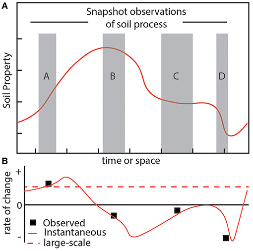
Figure 1. The problem of scale-dependent soil variability emerges in part due to a violation of equilibrium assumptions. (A) Consider a hypothetical soil property, such as carbon content, which is not in equilibrium and whose dynamics are represented by a plot of the auto-correlation values across time or space (solid orange line). Actual observations of this property are limited to finite spatial or temporal scales (gray boxes), though serve as the basis for characterizing the system state and its relationship to this hypothetical property. (B) Using the snapshot observations (gray boxes) to calculate meaningful system parameters (small black boxes), such as carbon turnover, illustrates how it would be difficult, if not impossible, to retrieve the hypothetical large-scale evolution (red dashed line) of the property which is increasing.

Equilibrium is often understood to connote a state of balance; e.g., equilibrium in a chemical reaction is a dynamic state in which the formation of products and reactants is balanced and time invariant. However, under non-equilibrium conditions the probabilistic relationships between energy and state break down; this could be because they are being driven away from equilibrium or because collective interactions among system components give rise to emergent states that are macroscopically “slow” to equilibrate, and highly variable at intermediate spatial or temporal scales (Cugliandolo et al., 1997; Kurchan, 1999). For example, macroscopic slowness in soils is exemplified by secondary mineral precipitation on mineral surfaces temporarily suppressing diffusion of primary mineral constituents into the soil solution (e.g., Velbel, 1993). In this scenario, the short-term rate of mineral dissolution is a function of both the soil solution itself (i.e., its degree of solute saturation and it's contact time) and the rate of surface rejuvenation. Thus, changing climates, chemical weathering dynamics, and biological/ecological processes such as ecological succession (Phillips, 2009; Lin, 2011; Yu and Hunt, 2018) can all be viewed as contributors to a system-level disequilibrium. While the aforementioned soil processes have received considerable attention, one whose effects are often overlooked is soil stirring.

Soils are being constantly perturbed and stirred by processes such as plant rooting, burrowing animals, freezing and thawing of water, and falling trees. Thus, soil stirring operates on a wide range of spatial and temporal scales (Figure 2) (Johnson et al., 2005; Wilkinson et al., 2009; Johnson and Schaetzl, 2015; Samonil et al., 2015). This process has underappreciated consequences with respect to soil disequilibrium because stirring causes bulk soil motion (BSM) which theoretically affects long-term rates of physical and chemical processes by controlling soil particle dynamics and the evolution of the soil's architecture (Figure 2). Expansion of the variety of methods for accurately determining pedoturbation rates over the last few decades has resulted in the growth of studies focusing on this soil process (Schaller et al., 2009; Stang et al., 2012; Johnson et al., 2014; Kristensen et al., 2015). What has emerged is not unexpected, for example, increasing soil stirring increases aggregate turnover, is associated with reduced soil horizonation, and increases chemical weathering and soil production rates (Wilkinson et al., 2009; Richards et al., 2011; Astete et al., 2016; Wackett et al., 2018). Taken together, the observed effects of soil stirring on soil processes align well with condensed matter theory, wherein a relationship has been demonstrated between stirring rate and a macroscopic system parameter known as the effective temperature, herein denoted as T* (Cohen et al., 2008; Cugliandolo, 2011).

FIGURE 2

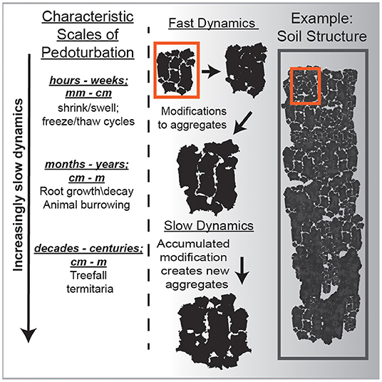
Figure 2. A conceptual illustration using soil aggregates to differentiate between the fast degrees of freedom vs. the slow degrees of freedom. Importantly, making a single measurement of the microscopic soil temperature using a dial thermometer would not reflect the dynamics which give rise to the slower processes. Rather you would have to measure the temperature over days, weeks, years to begin to capture those long-term dynamics such as shrink/swell or freeze/thaw.

The effective temperature is a macroscopic measure of the collective processes which control the large-scale relationship between state and energy in systems which violate the equilibrium condition of equipartition of energy (EoE) (Sornette, 2000; Cugliandolo, 2011). Physical systems to which T* has been successfully applied include glasses, polymers, granular matter, biological cells, collective behavior of organisms, and even brain activity (e.g., Langer and Manning, 2007; Wang et al., 2008; Loi et al., 2011a). While the connection between these examples and soil may not be immediately apparent, all of these systems, including soils, violate the principle of EoE because they are either being “driven/stirred", or the relaxation timescales following a perturbation are large relative to experimental observation. Because soils are both stirred and respond slowly to perturbations, suggests that T* is not only applicable to the study of soils, but that it may be used to recover energetic partitioning across large spatial (i.e., 10²⁻³ m) or temporal (i.e., 10²⁻³⁺yrs) scales. This is because path functions, such as the total chemical work done on a soil system over some time period, is a function of the temporal evolution of a few macroscopic state variables (e.g., temperature, pressure, volume). Because these state variables are not independent and are actually interrelated (e.g., PV = nRT), this implies that a soil's state and the associated path functions can be wholly described using a small number of interrelated state variables.

To summarize the preceding argument:

1. That the complexities we observe in soil processes are related to non-equilibrium state of most soil systems.

2. That rectifying this disequilibrium is required to mechanistically (through thermodynamics) extrapolate experimental observations of small-scale soil dynamics to large spatial and temporal scales.

3. That complex soil processes (e.g., chemical weathering) can be quantified using a small number of state variables, one of which is the non-equilibrium temperature.

4. That the non-equilibrium temperature is controlled by soil stirring (aka pedoturbation), which creates a bulk soil motion.

Because the foundations of this work are relatively unknown within the field of soil science this paper principally establishes the theoretical underpinnings of temperature and T*, and the relationship to soil processes. Ideally it serves as both a road map for the development of a modeling framework for overcoming the scaling gap and to establish a new theoretical approach to conceptualizing soils, namely as a macroscopic form of condensed matter.

2. Theory

2.1. Terminology

This work draws on ideas from the field of theoretical physics and is described using terms which may be new or used in ways unfamiliar to many readers. For the sake of clarity, a brief list of definitions is included below.

• Degrees of Freedom (d.f.): herein d.f. is used in the statistical mechanics sense, wherein d.f. refers to an ensemble of microstates or ‘microscopic' configurations of a system whose probability distribution gives rise to the value of a macrostate such as pressure, temperature, or density.

• Dynamics: Changes of a system or its components in response to a driver.

• Fast dynamics: Those dynamics of a system whose full response to a perturbation occurs over a period of experimental observation.

• Slow dynamics: Dynamics of a system whose full response to a perturbation does not occur over a period of experimental observation.

• Microscopic degrees of freedom: The degrees of freedom in a system which accommodate the fast dynamics. In soils these include primary particle positions, momenta, perhaps even mineralogy.

• Macroscopic degrees of freedom: The degrees of freedom in a system whose response is the result of the collective responses among the microscopic d.f., thus corresponding to the slow dynamics of a system. In the case of soils, these include bulk density, T*, and volume.

• Langevin dynamics: Dynamics which are said to be Langevin can be described using a stochastically perturbed differential equation (langevin equation; see Equations 5 and 6). Where the stochastic perturbations correspond to fast d.f., and the differential corresponds to slow d.f.

3. Temperature and Probability

Over the last few decades, theoretical developments in physics have demonstrated that a generalized formulation of temperature allows for the recovery of thermodynamic relationships by quantifying the “slow” processes affecting energetic partitioning. Under equilibrium conditions temperature is a thermodynamic parameter relating the average energy of a physical system as a whole, to a probabilistic distribution (partitioning) of energy among system states (Cugliandolo et al., 1997; Sornette, 2000). This statistical basis of thermodynamics is reflected in the following definition of temperature, where temperature is “a parameter which measures the amplitude of the noise or fluctuations of physical variables around their most probable state” (emphasis added) (Sornette, 2000). Thus, at its basis, temperature (T) is a probabilistic view of the energetics of a many-bodied system.

3.1. Temperature and Probability: The Equilibrium Case

Under equilibrium conditions, temperature relates the free energy of a system to the average energy (E) spread over the components comprising the system (Equation 1).

$\begin{array}{ll}E=-k_{B}TlnZ& (1)\end{array}$

For a given system, a change in T for some change of E, is proportional to the partitioning of energy across the ensemble of system microstates, with the partition function (Z) defining the ensemble itself (Equation 2) (Sornette, 2000). The Boltzmann constant, k_B [JK⁻¹], which is introduced for dimensionality, reflects that the probability of observing a particular microstate of the ensemble at energy E, is dependent on the Boltzmann distribution (Equation 2b).

$\begin{array}{ll}Z={\displaystyle \sum _i}P(E_i),& (\mathrm{2a})\end{array}$

$\begin{array}{ll}whereP(E)=e^{-\beta E}& (\mathrm{2b})\end{array}$

Thus as energy increases, the probability (P) of observing a system component with energy E, decreases exponentially, with β being inversely proportional to temperature (Equation 3), meaning that an increase in temperature is accompanied by a increase in the degrees of freedom accessible to the system (Sornette, 2000).

$\begin{array}{ll}T\equiv \frac{1}{k_B\beta }& (3)\end{array}$

Additionally, by substituting Equation (3) into Equation (2b) we can describe the Boltzmann distribution in terms of temperature (Equation 4).

$\begin{array}{ll}P(E)=e^{-\frac{1}{T{k}_b}E}& (4)\end{array}$

Thereby demonstrating that at it's core, temperature is a system-level metric which reflects the partitioning of energy and therefore ability of the system constituents to access different degrees of freedom. An important detail here is that this concept of temperature is almost exclusively thought of in terms of microscopic phenomena; e.g., the speed and collisions of gas atoms or the vibrational/rotational energy of molecules. Yet, the goal of the next section is to demonstrate that the abstract foundation of temperature can be used to quantify the dynamics of much larger systems, including non-equilibrium systems such as soils.

3.2. Deriving an Effective Temperature for Soils, the Non-equilibrium Case

The previous section demonstrates that for a generic system in thermodynamic equilibrium, a system's energy is related to its temperature. However, almost no physical system is truly in thermodynamic equilibrium (Cugliandolo, 2011). Under non-equilibrium conditions, such as systems with changing energy inputs (driving), or whose response times are long (kinetically locked) relative to observational timescales, the relationship between temperature and state cannot be treated statistically due to “faster” and “slower” dynamics controlling the partitioning of energy and the system state (Sornette, 2000; Jones, 2002; Cugliandolo, 2011). Regardless of whether the system is kinetically locked, or because the system is being driven, the ambient temperature (also known as the bath temperature) fails to describe the system thermodynamically, whereas the effective temperature, T*, does. To demonstrate why that is, in the following section, we closely followed the derivation established by Cugliandolo et al., for T* in generic, gently “stirred” systems (Cugliandolo et al., 1997; Kurchan, 1999; Cugliandolo, 2011).

3.2.1. Defining the System

The time-integrated stirring rate (D) describes the work which is done to drive a system from equilibrium, theoretically controlling the effective temperature. For simplicity, consider a soil system (i.e., a volume of soil) comprised of a number (N) of slow variables (e.g., chemical potential, viscosity, bulk density, or thermal conductivity) whose dynamic states (s_i….s_N) can be described by a generic Langevin equation of the form:

$\begin{array}{ll}{s}_i=b_i(s)+{\eta }_i(t),& (5)\end{array}$

wherein η_i(t), describes the fast variables of the system which are represented as Gaussian (thermal) noise. When the system responds to outside energy in a purely relaxational sense, this allows for the description of the average value of b_i as being proportional to the energy gradient of the Hamiltonian E(s), which has the general form:

$\begin{array}{ll}{b}_i(s)=-{\displaystyle \sum _j}{\Gamma }_{ij}\frac{\partial E(s)}{\partial s_j}.& (6)\end{array}$

The symmetric matrix, Γ_ij, relates the average value of the correlation function of the noise, η, over many realizations (denoted in angular brackets),

$\begin{array}{ll}\langle {\eta }_i(t){\eta }_j(t^{\prime })\rangle =2T_B{\Gamma }_{ij}\delta (t-t^{\prime }),& (7)\end{array}$

to the bath temperature which is a functionally limitless thermal mass in contact with the system, where δ denotes the Dirac delta function, and assuming 〈η_i(t)〉 = ∀i, t. The units of temperature are such that k_B is equal to 1 and therefore the equilibrium distribution is proportional to exp(-E/T).

3.2.2. Macroscopic Correlation and T*

Having defined the system in the previous section, it is now possible to gain insight into energy partitioning dynamics through the behavior of two observables, denoted as O₁ and O₂. In case of soils, two good choices could be bulk density (denoted as rho_b) and particle velocities (denoted v_b). Given that we are considering the non-equilibrium case where the temporal evolution is non-stationary, we define two times; an initial time, t₀, and a latest time, t. Using the observables, we construct a correlation function defined as C₁₂(t, t₀) ≡ 〈O₁(t)O₂(t₀) 〉 −〈O₁(t)〉〈O₂(t₀)〉, followed by their joint response as

$\begin{array}{ll}{R}_{12}(t,t_0)\equiv \frac{\delta O_1(t)}{\delta h_2(t_0)},& (8)\end{array}$

where h₂ appears as a perturbation in the Hamiltonian of the form E → E−h₂(t)O₂, and where O₂ is the observable receiving the perturbation. Which in the case that O₂ is bulk density, a perturbation would represent a functionally instantaneous localized compression or dilation. The time-integrated mutual response between the two observables (susceptibility) is further defined as:

$\begin{array}{ll}{\chi }_{12}(t,t_0)={\displaystyle {\int }_t^{t_0}}d{t}^{\prime }{R}_{12}(t,t^{\prime }).& (9)\end{array}$

Finally, the evolution of the correlation function values are used to construct the effective temperature (T*) through the integrated susceptibility (Equation 10) (Cugliandolo et al., 1997; Loi et al., 2011a),

$\begin{array}{ll}{\chi }_{12}(t-t_0)=\frac{1}{T*}\left[C_{12}(0)-C_{12}(t-t_0)\right].& (10)\end{array}$

By rearranging Equation (10), an equation for calculating T* is obtained:

$\begin{array}{ll}T*=\frac{\left[C_{12}(0)-C_{12}(t-t_0)\right]}{{\chi }_{12}(t-t_0)}.& (11)\end{array}$

Thus, the effective temperature, just like an equilibrium temperature, is a measurement of correlation and thus reorganizational dynamics of a system. In the case of soil science this means that the effective temperature is a measure of scale-dependent correlation in soil states and that it can by used to bound the scales at which short-term, small-scale observations of soil properties can be extrapolated. Because T* is a proper temperature, it can be used to recover thermodynamic relationships which are otherwise formally only permitted in the equilibrium case. It is worth emphasizing that soil properties which are intensive (i.e., their value is a local bulk phenomena) such as bulk density and velocity are those which may be used as observables for calculating the effective temperature.

4. Measuring Effective Temperatures

The equations presented in section 3.2 are presented to convey the conceptual underpinnings of T* and the quantitative basis for calculating and measuring it. Numerically calculating T* for very well-defined systems is relatively tractable and straightforward using computational simulations (Loi et al., 2011a). However, in the case of soils, we do not have much of the information needed to parameterize the full system of equations (e.g., Langevin equations) for calculating T* a priori given a defined pedoturbation/soil stirring rate. Alternatively, by measuring both the soil stirring rate and it's effect on soil state decorrelation (i.e., T*), it becomes possible to bound the estimates of parameter values within the langevin formalism. Furthermore, once we are able to predict T* for a range of soil stirring rates, and we know the controls of those stirring rates (e.g., bioturbation, freeze-thaw), then this opens the door to accurately and efficiently modeling the spatial and temporal evolution of dynamic soil properties using thermodynamic equations of state. Therefore, an initial step is to first measure the effective temperature using the right “thermometer,” which in practice is constructed by observing the dynamics of a tracer.

4.1. Developing a Tracer

Tracers used for investigating soil particle dynamics have been classified into two broad categories; native and exotic (Hardy et al., 2018). Native tracers rely on distinctive properties allowing the tracer to be related back to a point of origin in time or space [e.g., a distinctive lithologic outcrop (Migon and Kacprzak, 2014) or chemical signatures (Astete et al., 2016)]. Exotic tracers on the other hand, are recognizably exogenous and have a known time and place of introduction, examples include fluorescent particles, rare-earth element (REE) doped particles, radionuclides, or exotic minerals (Kimoto et al., 2006; Blake et al., 2009; Schlueter and Vogel, 2016; Hardy et al., 2018). Native tracers potentially enable larger intervals of time to be explored across a wide variety of landscapes (>100 yrs.), whereas exotic tracers potentially enable greater insight into the dynamics which are relevant on many experimental timescales (years-decades). However, to effectively measure T*, tracers need to couple to the reorganizational dynamics of the system microstates (Loi et al., 2011a), such as the metastable aggregates of primary soil particles. In practice, most tracer-based determinations of the effective temperature are constructed by observing the spatial and temporal changes in the velocities and positions of the tracers particles.

Regardless of whether the tracer is exotic or native, the calculated value of the effective temperature is can be sensitive to the tracer properties such as mass or volume (Cugliandolo et al., 1997; Loi et al., 2011b). Using a computational simulation of a model system, Loi et al. (2011b) demonstrated that the calculated value of T* is non-linearly dependent on tracer mass (Figure 3) (Loi et al., 2011a,b). Within their model polymer system, the mass-dependent value of T* arises because the more massive tracer integrates a larger number of particle collisions. Thus the findings of Loi et al. suggest that regardless of native vs. exotic tracers, the recovered value of T* will depend on which components of the system the tracer couples with, with smaller tracers coupling with faster degrees of freedom.

FIGURE 3

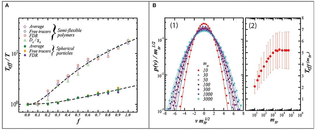
Figure 3. Two figures from Loi et al. (2011b). (A) Relationship between the recovered value of T* (i.e., T_eff) relative to the bath temperature (T) vs. the dimensionless driving strength (f) from two model configurations: one comprised of flexible polymers of 21 units long, the other of hard spheres. Values which are plotted are the average of T_eff/T derived from motorized tracers (diamonds), from free tracers (circles), the fluctuation-dissipation ratio (squares), and in the case of the semi-flexible polymers, the ratio of the diffusion coefficient (D_x) to the susceptibility (X_x). Importantly, this figure highlights that the internal degrees of freedom (i.e., flexible vs. hard sphere) have the potential to differentially affect the value of T* which is retrieved for a given driving rate. In the context of soils, this figure provides evidence that the temperature sensitivity of soil dynamics (akin to a heat capacity), depend on the soil properties (such as texture) which affect the internal degrees of freedom of the soil (B): (1) Graph of the probability distribution of the velocity (p(v)) plotted vs. the scaled velocity (vm^1/2), where v is the velocity and m is the mass of the tracer. (2) The effective temperature of the tracer particle as extracted from the velocity data and plotted as a function of tracer mass. The model predicts that the variance and absolute value of T* increases with increasing tracer mass, eventually saturating at 50x the mass of the 21-unit polymer. These modeling results suggest that within soil, less massive tracers are more prone to self-diffusion and therefore underestimate the long-term stirring rates and the effective temperature. Both figures reprinted from Loi et al. (2011b), courtesy of the Royal Society of Chemistry.

Many studies have applied tracers to the study of soil dynamics and bulk soil motion/stirring. However, for the purposes of calculating the effective temperature, more information is needed than is typically collected, such as the time evolution of tracer velocities, and their positions. Additionally, the properties of the tracers themselves, such as their mass, in some cases affect the tracer behavior. Case in point is the work of Loi et al. (2011b) wherein they evaluate the effect of geometry and mass on the recovered velocities and mean-squared displacements of a motorized tracers (Figure 3). Taken together, this means that the existent tracer studies likely only capture a fraction of the dynamics needed to calculate T*, making it difficult to rely wholly on the existing literature to compile estimates of the effective temperatures (Cugliandolo et al., 1997). Thus new tracers need to be developed which allow for their positions and velocities to be non-destructively observed. Once such tracers have been developed, they can then be deployed across a range of soil types and soil stirring rates in order to quantify T* in the long-time limit and its sensitivity to soil properties (such as clay content and mineralogy) and environmental drivers.

5. Discussion and Conclusions

5.1. Initial Applications of T* in Soils

The theoretical framework presented here is a simplification and there are many outstanding questions regarding the bounds of application. For one, measurement of T* itself does not directly quantify the rates of soil processes, rather it provides a fundamental measure of a soil system which can be used to account for emergent properties, such as self-assembly of soil aggregates and their effect on the dynamics of soil formation. Furthermore, because the effective temperature is a macroscopic feature of microscopic soil variables, a new mechanistic approach to extending measurements of small scale processes to larger spatial and temporal scales will be needed. Nevertheless, simplifying complex soil dynamics and casting them in the light of thermodynamics has the potential to improve a wide variety of challenges within the field of soil science. This potential emerges in part because T* parameterizes the “slow” processes of energetic partitioning, which are processes which affect how energy is distributed among the suite of contributors to a soil's energy state, such as its mechanical, chemical, electrical, or even gravitational energies. For example, imagine a soil wherein reduced oxygen in the subsurface is impeding organic matter degradation. The pool of chemical energy stored in the organic matter can be seen as a slow variable which is in meta-stable equilibrium with the current configuration of the oxygen concentration gradient. Where T* quantifies the potential for soil particles to change their position, and thus the organic matter's potential for changing location with respect to the oxygen gradient, thus T* provides a metric of the potential for that chemical energy to be converted to some other form of energy in the soil system. Below we present three examples of currently pressing topics which appear poised to benefit from this approach; relaxational dynamics, aggregate turnover and carbon cycling, and soil erosion/production.

5.1.1. Soil Memory and Relaxation

While T* has yet to be measured in soils, soil relaxation dynamics which are theoretically sensitive to T* have been observed. Relaxation times of soil properties have been calculated using soil microtopography (Schaetzl et al., 1989; Jyotsna and Haff, 1997; Pawlik, 2013; Samonil et al., 2015), erasure of compaction events (Pfahler et al., 2015; Keller et al., 2017; Schlueter et al., 2018), vegetation changes (Phillips, 2009; Nauman et al., 2015), and landform evolution (Fernandes and Dietrich, 1997; Gabet, 2000; Phillips and Marion, 2004; Pelletier et al., 2006; Hoffman and Anderson, 2014). These studies together provide evidence that relaxation times are not uniform; though the cause of the non-uniformity remains unclear. For example, estimates of relaxation times following soil compaction range from in excess of 125 years in the Mojave Desert (USA), 25 years for a soil in Northern Germany, and 30 years in the Russian steppe (Webb, 2002; Kalinina et al., 2015; Schlueter et al., 2018). Intriguingly, in most studies, mechanisms which are equivalent to soil stirring (esp. bioturbation) are prominently considered as affecting the relaxation dynamics of their system. These observations provide anecdotal evidence that differences in relaxation times are related to the effective temperature of a system. Thus by quantifying T* for a range of soil types and stirring rates, we can begin comparing the underlying causes of differential relaxation times (see section 3.2.2) and thereby estimate the timescales of soil memory and the controls thereof.

The relationship between the effective temperature and the response times of soil to a perturbation, such as a compaction event or displacement due to a tree uprooting, can be quantified in a variety of ways. In the case of compaction, it useful to estimate the time it takes for the soil to revert, t_R, to the pre-compacted density. If we assume that soils are below the critical temperature which demarcates the onset of glassy dynamics, then the reversal time is Arrheniusly dependent on the effective temperature and the spatially extensive free energy barrier (ΔF) between the compacted and un-compacted states (Equation 12) (Cugliandolo, 2013).

$\begin{array}{ll}{t}_R=e^{\frac{1}{T*}\Delta F}.& (12)\end{array}$

By directly measuring the reversal time in conjunction with the effective temperature, it becomes possible to quantify an otherwise difficult to estimate value: the free energy barrier between the two configurations (i.e., compacted and un-compacted). From a practical perspective, one example of the use in determining the value of ΔF is that it provides a measure of energetic costs associated with reclaiming compacted soil. Alternatively, if the energy barrier can be estimated a priori and T* is known, then calculating the lifespan and thus the memory of a perturbation to a soil property is relatively straightforward.

5.1.2. Integrating Aggregate Turnover Within Carbon Cycling Models

Many soil processes are affected by aggregate dynamics, including soil hydrology, redox status, C and N turnover, and microbial communities (Six et al., 2004; Keller et al., 2017; Almquist et al., 2018; Baveye et al., 2018; Keiluweit et al., 2018). Carbon turnover rates often do not respond to ambient temperature changes (i.e., microscopic temperature) (Six et al., 2004; Hamdi et al., 2013; Torres-Sallan et al., 2018). This mismatch has led to the conclusion that C-cycling in soils may not be thermodynamically limited, but rather that it is kinetically limited. Furthermore, kinetic limitations of C-turnover are linked to carbon sorption on particles [e.g., Crow and Sierra (2018)] and processes of aggregation (Kalinina et al., 2015; Crow and Sierra, 2018). However, because the effective temperature and the aggregate turnover are controlled by BSM, and that in the longtime limit C-mobility is essentially diffusive, this implies that carbon turnover rate is proportional to the effective temperature (Equation 13) through the temperature dependency of diffusion itself (Loi et al., 2011a). Thus in practical terms, this implies that once the controls on T* are known, dynamically modeling C-turnover across a wide range of temporal and spatial scales can be accomplished simply by estimating T*.

5.1.3. Beyond the Soil Production Function

In addition to aggregate turnover, soil stirring has been observed to control a significant portion of soil flux on hillslopes over long timescales (Roering et al., 2002; Gabet et al., 2003; Wilkinson et al., 2009; Pawlik and Samonil, 2018). Long-term soil flux is commonly quantified using the cosmogenic radionuclide-based estimates of denudation and the soil production function (SPF). The SPF is an empirical function which provides estimates hillslope soil flux, and in so doing, forms a critical linkage between fluvial incision and the associated geomorphic response of a landscape on long timescales (> 10⁴ yrs) (Heimsath et al., 1997; Humphreys and Wilkinson, 2007; Nicotina et al., 2011). Soil flux is generally assumed to be diffusive, and controlled primarily by the local hillslope gradient (Heimsath et al., 2001; Gabet et al., 2003; Wilkinson and Humphreys, 2005; Gabet and Mudd, 2010; Riebe et al., 2015; Wackett et al., 2018). A concerted effort to measure soil production rates at various sites around the world (Table 1) raises doubt that the assumption that hillslope gradient controls the flux and diffusion rates (Figure 4). Instead, on low-relief portions of the terrestrial surface (which is arguably more than 90% of the land surface; Willenbring et al., 2013), climate and biology may control soil mobility (Figure 4) just as strongly, if not more so than topography.

TABLE 1

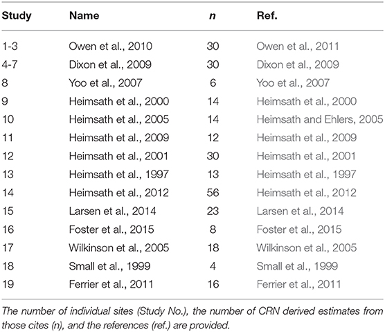
Table 1. Global compilation of geo-referenced CRN-derived denudation rates used to calculate soil mass diffusivities reported in Figure 4.

FIGURE 4

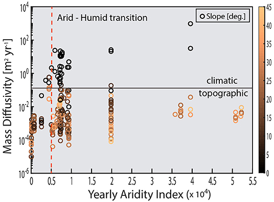
Figure 4. Global compilation of soil mass diffusivity values plotted against the CGIAR yearly average aridity index for each site appear to display differential sensitivity to climate and slope. This figure demonstrates that topographic parameters such as slope or curvature only explain a fraction of the mechanisms of “diffusion.” Geomorphologists and soil scientists have sought to deconvolve the contributions of biota to climatic sensitivity observed in diffusion-like soil movement, though with limited success. However, by relating stirring rate to T*, this provides a new tool in separating abiotic vs. biotic drivers of climate sensitivity brought about by soil stirring. See Appendix for details of data compilation and equations for calculating mass diffusivity.

Despite climate and biota playing a primary role in denudation, topographic derivatives such as hillslope gradient and curvature are the primary means of extrapolating site-level denudation rates to the landscape scale. However, as Figure 4 demonstrates, using topography to estimate mass transport at the global level is seriously hindered by the presence of lower order controls (e.g., climate) on transport and diffusion. Thus, the lack of a unifying parameter in estimating diffusive rates is problematic for integrating denudatative fluxes, which is on long timescales (10⁶⁻⁸ yrs), are achieved primarily due to relatively slow, diffusive/advection processes (e.g., BSM) (Fernandes and Dietrich, 1997; Furbish and Fagherazzi, 2001; Heimsath et al., 2001; Furbish et al., 2009; Bonetti and Porporato, 2017).

Diffusion is a temperature dependent process, including for T*. Where the bath temperature (T_B) is known, the diffusion coefficient of a massive tracer (Dρ) is then related to the effective temperature by Equation (13) (Loi et al., 2011b).

$\begin{array}{ll}\frac{D\rho }{T_B}\propto {\left(\frac{T*}{T_B}\right)}^{\alpha }& (13)\end{array}$

Because soil displacement is diffusive in the long-time limit, this suggests that hillslope soil transport and soil production rates can be estimated a priori using T* once the controls on T* are known. Measurements of soil diffusivity have primarily relied on a post-hoc calculation of diffusivity using CRN-derived estimates of denudation and by assuming steady-state soil thickness. Currently, despite potentially problematic assumptions of steady-state thickness, a significant number of these studies indicate that biota strongly affect soil diffusivity. Yet the exact mechanisms or and magnitude of biotically driven soil diffusion is obscured by the fact that CRN inventories typically integrate over significant periods of climate and ecosystems variability (Wilkinson et al., 2005; Dietrich and Perron, 2006; Lin, 2011; Amundson et al., 2015). Yet because T* is proportional only to the driving/stirring rate and the susceptibility, this provides a complimentary tool for deconvolving the biotic and abiotic drivers of climatic sensitivity observed in long-term CRN-derived estimates of diffusivity.

5.1.4. Thermodynamic and Condensed Matter Models of Soils

Thermodynamic solutions to complex soil dynamics, especially those of pedogenesis, have been proposed numerous times over the last half century, examples include that of Nikiforoff (1959) and more recently that of Rasmussen (2012) and of Lin (2011). Yet these models have more or less encountered the same limitation; what to do about non-equilibrium and the discrepancy between fast and slow processes (Lin, 2011). One approach is to define the system over a scale in time or space which permits a quasi-equilibrium assumption. While this scale-dependent equilibrium allows for thermodynamics to be used, it remains difficult to integrate any findings into a broader understanding of soil dynamics because of the scaling gap which was necessarily assumed away. However, if T* can be used to reconcile the slow and fast components of energetic partitioning in soil, then it offers the opportunity to transcend the current scaling limitations preventing the holistic application of thermodynamic and statistical mechanical principles to the study of soil dynamics. However, in addition to reconciling thermodynamic approaches to the study of soils as energetically open systems, quantifying T* has the potential to answer a very fundamental question: can soil be viewed as an ultra-macroscopic form of condensed matter? If so, what would be the significance and the implications which would be borne out of this discovery?

5.2. Summary and Conclusions

Despite the fact that for more than a century, soil stirring has been documented to affect a wide variety of soil processes, it has never been considered as if it gave rise to a soil temperature. The argument presented herein is that experimental observations of soils are consistent with stirring playing the role of an effective temperature. The recovery of thermodynamic relationships using the effective temperature provides a new tool set for not only studying the long-time evolution of soil properties, but also mechanistically enabling extrapolation of laboratory-scale observations to landscape-scale soil processes. While the theoretical framework clearly exists for extending thermodynamics to understand macroscopic systems, doing so in soil will require a concerted effort to construct new measurement approaches. For instance, tracer-based approaches will need to be carefully considered because the recovered value of T* is sensitive to the physical properties (see section 4.1) of the tracer. Nevertheless, because T* is a true temperature, meaning that it describes the relationship between entropy and energy, it allows for a variety macroscopic soil properties (such as viscosity or pressure) to be calculated which were formerly inapplicable to understanding soils, the dynamics of their formation, and predicting their future evolution.

Data Availability Statement

Publicly available datasets were analyzed in this study. This data can be found here: https://ir.library.oregonstate.edu/concern/datasets/7h149w15g.

Author Contributions

VA conceived, wrote, and prepared the manuscript in its entirety.

Conflict of Interest

The author declares that the research was conducted in the absence of any commercial or financial relationships that could be construed as a potential conflict of interest.

Acknowledgments

The author would like to acknowledge Drs. Stephany Chacon, Jason Kelley, Maria Dragila, and Markus Kleber for providing helpful conversations, edits, and difficult questions, which greatly improved this manuscript. I would also like to acknowledge the support and encouragement of Dr. Jay Noller and Edgar Velásquez.

References

Almquist, V., Brueck, C., Clarke, S., Wanzek, T., and Dragila, M. I. (2018). Bioavailable water in coarse soils: a fractal approach. Geoderma 323, 146–155. doi: 10.1016/j.geoderma.2018.02.036

CrossRef Full Text | Google Scholar

Amundson, R., Heimsath, A., Owen, J., Yoo, K., and Dietrich, W. E. (2015a). Hillslope soils and vegetation. Geomorphology 234, 122–132. doi: 10.1016/j.geomorph.2014.12.031

CrossRef Full Text | Google Scholar

Astete, C. E., Thibodeaux, L. J., and Constant, W. D. (2016). Semi-volatile organic compounds as chemical tracers for estimating soil particle biodiffusion coefficients: application of polychlorinated biphenyls in earthworm bioturbation at a grassland site. Soil Sci. 181, 457–464. doi: 10.1097/SS.0000000000000178

CrossRef Full Text | Google Scholar

Baveye, P. C., and Laba, M. (2015). Moving away from the geostatistical lamppost: why, where, and how does the spatial heterogeneity of soils matter? Ecol. Modell. 298, 24–38. doi: 10.1016/j.ecolmodel.2014.03.018

CrossRef Full Text | Google Scholar

Baveye, P. C., Otten, W., Kravchenko, A., Balseiro-Romero, M., Beckers, E., Chalhoub, M., et al. (2018). Emergent properties of microbial activity in heterogeneous soil microenvironments: different research approaches are slowly converging, yet major challenges remain. Front. Microbiol. 9:1929. doi: 10.3389/fmicb.2018.01929

PubMed Abstract | CrossRef Full Text | Google Scholar

Blake, W. H., Wallbrink, P. J., Wilkinson, S. N., Humphreys, G., Doerr, S. H., Shakesby, R. A., et al. (2009). Deriving hillslope sediment budgets in wildfire-affected forests using fallout radionuclide tracers. Geomorphology 104, 105–116. doi: 10.1016/j.geomorph.2008.08.004

CrossRef Full Text | Google Scholar

Bonetti, S., and Porporato, A. (2017). On the dynamic smoothing of mountains. Geophys. Res. Lett. 44, 5531–5539. doi: 10.1002/2017GL073095

CrossRef Full Text | Google Scholar

Cohen, S., Willgoose, G., and Hancock, G. (2008). A methodology for calculating the spatial distribution of the area-slope equation and the hypsometric integral within a catchment. J. Geophys. Res. Earth Surf. 113. doi: 10.1029/2007JF000820

CrossRef Full Text | Google Scholar

Crow, S. E., and Sierra, C. A. (2018). Dynamic, intermediate soil carbon pools may drive future responsiveness to environmental change. J. Environ. Qual. 47, 607–616. doi: 10.2134/jeq2017.07.0280

PubMed Abstract | CrossRef Full Text | Google Scholar

Cugliandolo, L. F. (2011). The effective temperature. J. Phys. A Math. Theor. 44. doi: 10.1088/1751-8113/44/48/483001

CrossRef Full Text | Google Scholar

Cugliandolo, L. F. (2013). Out-of-equilibrium dynamics of classical and quantum complex systems. C R Phys. 14, 685–699. doi: 10.1016/j.crhy.2013.09.004

CrossRef Full Text | Google Scholar

Cugliandolo, L. F., Kurchan, J., and Peliti, L. (1997). Energy flow, partial equilibration, and effective temperatures in systems with slow dynamics. Phys. Rev. E 55, 3898–3914. doi: 10.1103/PhysRevE.55.3898

CrossRef Full Text | Google Scholar

Cushman, J. H., and O'Malley, D. (2015). Fickian dispersion is anomalous. J. Hydrol. 531, 161–167. doi: 10.1016/j.jhydrol.2015.06.036

CrossRef Full Text | Google Scholar

Dietrich, W. E., and Perron, J. T. (2006). The search for a topographic signature of life. Nature 439, 411–418. doi: 10.1038/nature04452

PubMed Abstract | CrossRef Full Text | Google Scholar

Dixon, J. L., Heimsath, A. M., and Amundson, R. (2009). The critical role of climate and saprolite weathering in landscape evolution. Earth Surf. Process. Landforms 34, 1507–1521. doi: 10.1002/esp.1836

CrossRef Full Text | Google Scholar

Fernandes, N. F., and Dietrich, W. E. (1997). Hillslope evolution by diffusive processes: the timescale for equilibrium adjustments. Water Resour. Res. 33, 1307–1318. doi: 10.1029/97WR00534

CrossRef Full Text | Google Scholar

Ferrier, K. L., Kirchner, J. W., and Finkel, R. C. (2011). Estimating millennial-scale rates of dust incorporation into eroding hillslope regolith using cosmogenic nuclides and immobile weathering tracers. J. Geophys. Res. Earth Surf. 116. doi: 10.1029/2011JF001991

CrossRef Full Text | Google Scholar

Foster, M. A., Anderson, R. S., Wyshnytzky, C. E., Ouimet, W. B., and Dethier, D. P. (2015). Hillslope lowering rates and mobile-regolith residence times from in situ and meteoric be-10 analysis, boulder creek critical zone observatory, colorado. Geol. Soc. Am. Bull. 127, 862–878. doi: 10.1130/B31115.1

CrossRef Full Text | Google Scholar

Furbish, D. J., and Fagherazzi, S. (2001). Stability of creeping soil and implications for hillslope evolution. Water Resour. Res. 37, 2607–2618. doi: 10.1029/2001WR000239

CrossRef Full Text | Google Scholar

Furbish, D. J., Haff, P. K., Dietrich, W. E., and Heimsath, A. M. (2009). Statistical description of slope-dependent soil transport and the diffusion-like coefficient. J. Geophys. Res. Earth Surf. 114. doi: 10.1029/2009JF001267

CrossRef Full Text | Google Scholar

Gabet, E. J. (2000). Gopher bioturbation: field evidence for non-linear hillslope diffusion. Earth Surf. Process. Landforms 25, 1419–1428. doi: 10.1002/1096-9837(200012)25:13<1419::AID-ESP148>3.0.CO;2-1

CrossRef Full Text | Google Scholar

Gabet, E. J., and Mudd, S. M. (2010). Bedrock erosion by root fracture and tree throw: a coupled biogeomorphic model to explore the humped soil production function and the persistence of hillslope soils. J. Geophys. Res. Earth Surf. 115. doi: 10.1029/2009JF001526

CrossRef Full Text | Google Scholar

Gabet, E. J., Reichman, O. J., and Seabloom, E. W. (2003). The effects of bioturbation on soil processes and sediment transport. Annu. Rev. Earth Planet. Sci. 31, 249–273. doi: 10.1146/annurev.earth.31.100901.141314

CrossRef Full Text | Google Scholar

Hamdi, S., Moyano, F., Sall, S., Bernoux, M., and Chevallier, T. (2013). Synthesis analysis of the temperature sensitivity of soil respiration from laboratory studies in relation to incubation methods and soil conditions. Soil Biol. Biochem. 58, 115–126. doi: 10.1016/j.soilbio.2012.11.012

CrossRef Full Text | Google Scholar

Hardy, R., Quinton, J., James, M., Fiener, P., and Pates, J. (2018). High precision tracing of soil and sediment movement using fluorescent tracers at hillslope scale. Earth Surf. Process. Landforms. 44, 1091–1099. doi: 10.1002/esp.4557

CrossRef Full Text | Google Scholar

Heimsath, A. M., Chappell, J., Dietrich, W. E., Nishiizumi, K., and Finkel, R. C. (2000). Soil production on a retreating escarpment in southeastern Australia. Geology 28, 787–790. doi: 10.1130/0091-7613(2000)28<787:SPOARE>2.0.CO;2

CrossRef Full Text | Google Scholar

Heimsath, A. M., DiBiase, R. A., and Whipple, K. X. (2012). Soil production limits and the transition to bedrock-dominated landscapes. Nat. Geosci. 5, 210–214. doi: 10.1038/ngeo1380

CrossRef Full Text | Google Scholar

Heimsath, A. M., Dietrich, W. E., Nishiizumi, K., and Finkel, R. C. (1997). The soil production function and landscape equilibrium. Nature 388, 358–361. doi: 10.1038/41056

CrossRef Full Text | Google Scholar

Heimsath, A. M., Dietrich, W. E., Nishiizumi, K., and Finkel, R. C. (2001). Stochastic processes of soil production and transport: erosion rates, topographic variation and cosmogenic nuclides in the oregon coast range. Earth Surf. Process. Landforms 26, 531–552. doi: 10.1002/esp.209

CrossRef Full Text | Google Scholar

Heimsath, A. M., and Ehlers, T. A. (2005). Quantifying rates and timescales of geomorphic processes. Earth Surf. Process. Landforms 30, 917–921. doi: 10.1002/esp.1253

CrossRef Full Text | Google Scholar

Heimsath, A. M., Fink, D., and Hancock, G. R. (2009). The ‘humped' soil production function: eroding arnhem land, Australia. Earth Surf. Process. Landforms 34, 1674–1684. doi: 10.1002/esp.1859

CrossRef Full Text | Google Scholar

Hoffman, B. S. S., and Anderson, R. S. (2014). Tree root mounds and their role in transporting soil on forested landscapes. Earth Surf. Process. Landforms 39, 711–722. doi: 10.1002/esp.3470

CrossRef Full Text | Google Scholar

Humphreys, G. S., and Wilkinson, M. T. (2007). The soil production function: a brief history and its rediscovery. Geoderma 139, 73–78. doi: 10.1016/j.geoderma.2007.01.004

CrossRef Full Text | Google Scholar

Johnson, D. L., Domier, J. E. J., and Johnson, D. N. (2005). Reflections on the nature of soil and its biomantle. Ann. Assoc. Am. Geograph. 95, 11–31. doi: 10.1111/j.1467-8306.2005.00448.x

CrossRef Full Text | Google Scholar

Johnson, D. L., and Schaetzl, R. J. (2015). Differing views of soil and pedogenesis by two masters: Darwin and dokuchaev. Geoderma 237, 176–189. doi: 10.1016/j.geoderma.2014.08.020

CrossRef Full Text | Google Scholar

Johnson, M. O., Mudd, S. M., Pillans, B., Spooner, N. A., Fifield, L. K., Kirkby, M. J., et al. (2014). Quantifying the rate and depth dependence of bioturbation based on optically-stimulated luminescence (OSL) dates and meteoric be-10. Earth Surf. Process. Landforms 39, 1188–1196. doi: 10.1002/esp.3520

CrossRef Full Text | Google Scholar

Jones, R. A. L. (2002). Soft Condensed Matter. New York, NY: Oxford University Press.

Google Scholar

Jyotsna, R., and Haff, P. K. (1997). Microtopography as an indicator of modern hillslope diffusivity in arid terrain. Geology 25, 695–698. doi: 10.1130/0091-7613(1997)025<0695:MAAIOM>2.3.CO;2

CrossRef Full Text | Google Scholar

Kalinina, O., Barmin, A. N., Chertov, C., Dolgikh, A. V., Goryachkin, S. V., Lyuri, D. I., et al. (2015). Self-restoration of post-agrogenic soils of Calcisol-Solonetz complex: Soil development, carbon stock dynamics of carbon pools. Geoderma 237, 117–128. doi: 10.1016/j.geoderma.2014.08.013

CrossRef Full Text | Google Scholar

Keiluweit, M., Gee, K., Denney, A., and Fendorf, S. (2018). Anoxic microsites in upland soils dominantly controlled by clay content. Soil Biol. Biochem. 118, 42–50. doi: 10.1016/j.soilbio.2017.12.002

CrossRef Full Text | Google Scholar

Keller, T., Colombi, T., Ruiz, S., Manalili, M. P., Rek, J., Stadelmann, V., et al. (2017). Long-term soil structure observatory for monitoring post-compaction evolution of soil structure. Vadose Zone J. 16, 1–16. doi: 10.2136/vzj2016.11.0118

CrossRef Full Text | Google Scholar

Kimoto, A., Nearing, M. A., Shipitalo, M. J., and Polyakov, V. O. (2006). Multi-year tracking of sediment sources in a small agricultural watershed using rare earth elements. Earth Surf. Process. Landforms 31, 1763–1774. doi: 10.1002/esp.1355

CrossRef Full Text | Google Scholar

Kristensen, J. A., Thomsen, K. J., Murray, A. S., Buylaert, J. P., Jain, M., and Breuning-Madsen, H. (2015). Quantification of termite bioturbation in a savannah ecosystem: Application of OSL dating. Q. Geochronol. 30, 334–341. doi: 10.1016/j.quageo.2015.02.026

CrossRef Full Text | Google Scholar

Kurchan, J. (1999). Emergence of macroscopic temperatures in systems that are not thermodynamical microscopically: towards a thermodynamical description of slow granular rheology. J. Phys. Cond. Matter 12, 6611–6617. doi: 10.1088/0953-8984/12/29/332

CrossRef Full Text | Google Scholar

Langer, J. S., and Manning, M. L. (2007). Steady-state, effective-temperature dynamics in a glassy material. Phys. Rev. E 76:056107. doi: 10.1103/PhysRevE.76.056107

PubMed Abstract | CrossRef Full Text | Google Scholar

Larsen, I. J., Almond, P. C., Eger, A., Stone, J. O., Montgomery, D. R., and Malcolm, B. (2014). Rapid soil production and weathering in the southern alps, new zealand. Science 343, 637–640. doi: 10.1126/science.1244908

PubMed Abstract | CrossRef Full Text | Google Scholar

Lin, H. (2011). Three principles of soil change and pedogenesis in time and space. Soil Sci. Soc. Am. J. 75, 2049–2070. doi: 10.2136/sssaj2011.0130

CrossRef Full Text | Google Scholar

Loi, D., Mossa, S., and Cugliandolo, L. F. (2011a). Effective temperature of active complex matter. Soft Matter 7, 3726–3729. doi: 10.1039/c0sm01484b

CrossRef Full Text | Google Scholar

Loi, D., Mossa, S., and Cugliandolo, L. F. (2011b). Non-conservative forces and effective temperatures in active polymers. Soft Matter 7, 10193–10209. doi: 10.1039/c1sm05819c

CrossRef Full Text | Google Scholar

Migon, P., and Kacprzak, A. (2014). Lateral diversity of regolith and soils under a mountain slope - implications for interpretation of hillslope materials and processes, central sudetes, SW Poland. Geomorphology 221, 69–82. doi: 10.1016/j.geomorph.2014.06.003

CrossRef Full Text | Google Scholar

Nauman, T. W., Thompson, J. A., Teets, S. J., Dilliplane, T. A., Bell, J. W., Connolly, S. J., et al. (2015). Ghosts of the forest: mapping pedomemory to guide forest restoration. Geoderma 247, 51–64. doi: 10.1016/j.geoderma.2015.02.002

CrossRef Full Text | Google Scholar

Nicotina, L., Tarboton, D. G., Tesfa, T. K., and Rinaldo, A. (2011). Hydrologic controls on equilibrium soil depths. Water Resour. Res. 47. doi: 10.1029/2010WR009538

CrossRef Full Text | Google Scholar

Nikiforoff, C. C. (1959). Reappraisal of the soil. Science 129, 186–196. doi: 10.1126/science.129.3343.186

PubMed Abstract | CrossRef Full Text | Google Scholar

Owen, J. J., Amundson, R., Dietrich, W. E., Nishiizumi, K., Sutter, B., and Chong, G. (2011). The sensitivity of hillslope bedrock erosion to precipitation. Earth Surf. Process. Landforms 36, 117–135. doi: 10.1002/esp.2083

CrossRef Full Text | Google Scholar

Pachepsky, Y., and Hill, R. L. (2017). Scale and scaling in soils. Geoderma 287, 4–30. doi: 10.1016/j.geoderma.2016.08.017

CrossRef Full Text | Google Scholar

Pawlik, L. (2013). The role of trees in the geomorphic system of forested hillslopes - a review. Earth Sci. Rev. 126, 250–265. doi: 10.1016/j.earscirev.2013.08.007

CrossRef Full Text | Google Scholar

Pawlik, L., and Samonil, P. (2018). Soil creep: the driving factors, evidence and significance for biogeomorphic and pedogenic domains and systems - A critical literature review. Earth Sci. Rev. 178, 257–278. doi: 10.1016/j.earscirev.2018.01.008

CrossRef Full Text | Google Scholar

Pelletier, J. D., DeLong, S. B., Al-Suwaidi, A. H., Cline, M., Lewis, Y., Psillas, J. L., et al. (2006). Evolution of the bonneville shoreline scarp in west-central utah: Comparison of scarp-analysis methods and implications for the diffusion model of hillslope evolution. Geomorphology 74, 257–270. doi: 10.1016/j.geomorph.2005.08.008

CrossRef Full Text | Google Scholar

Pfahler, V., Glaser, B., McKey, D., and Klemt, E. (2015). Soil redistribution in abandoned raised fields in French Guiana assessed by radionuclides. J. Plant Nutr. Soil Sci. 178, 468–476. doi: 10.1002/jpln.201400279

CrossRef Full Text | Google Scholar

Phillips, J. D. (2009). Soils as extended composite phenotypes. Geoderma 149, 143–151. doi: 10.1016/j.geoderma.2008.11.028

CrossRef Full Text | Google Scholar

Phillips, J. D., and Marion, D. A. (2004). Pedological memory in forest soil development. Forest Ecol. Manage. 188, 363–380. doi: 10.1016/j.foreco.2003.08.007

CrossRef Full Text | Google Scholar

Rasmussen, C. (2012). Thermodynamic constraints on effective energy and mass transfer and catchment function. Hydrol. Earth Syst. Sci. 16, 725–739. doi: 10.5194/hess-16-725-2012

CrossRef Full Text | Google Scholar

Richards, P. J., Hohenthal, J. M., and Humphreys, G. S. (2011). Bioturbation on a south-east Australian hillslope: estimating contributions to soil flux. Earth Surf. Process. Landforms 36, 1240–1253. doi: 10.1002/esp.2149

CrossRef Full Text | Google Scholar

Riebe, C. S., Sklar, L. S., Lukens, C. E., and Shuster, D. L. (2015). Climate and topography control the size and flux of sediment produced on steep mountain slopes. Proc. Natl. Acad. Sci. U.S.A. 112, 15574–15579. doi: 10.1073/pnas.1503567112

PubMed Abstract | CrossRef Full Text | Google Scholar

Roering, J. J., Almond, P., Tonkin, P., and McKean, J. (2002). Soil transport driven by biological processes over millennial time scales. Geology 30, 1115–1118. doi: 10.1130/0091-7613(2002)030<1115:STDBBP>2.0.CO;2

CrossRef Full Text | Google Scholar

Samonil, P., Danek, P., Schaetzl, R. J., Vasickova, I., and Valtera, M. (2015). Soil mixing and genesis as affected by tree uprooting in three temperate forests. Eur. J. Soil Sci. 66, 589–603. doi: 10.1111/ejss.12245

CrossRef Full Text | Google Scholar

Schaetzl, R. J., Johnson, D. L., Burns, S. F., and Small, T. (1989). Tree uprooting - review of terminology, process, and environmental implications. Canad. J. For. Res. 19, 1–11. doi: 10.1139/x89-001

CrossRef Full Text | Google Scholar

Schaller, M., Ehlers, T. A., Blum, J. D., and Kallenberg, M. A. (2009). Quantifying glacial moraine age, denudation, and soil mixing with cosmogenic nuclide depth profiles. J. Geophys. Res. Earth Surf. 114. doi: 10.1029/2007JF000921

CrossRef Full Text | Google Scholar

Schlueter, S., Grossmann, C., Diel, J., Wu, G.-M., Tischer, S., Deubel, A., et al. (2018). Long-term effects of conventional and reduced tillage on soil structure, soil ecological and soil hydraulic properties. Geoderma 332, 10–19. doi: 10.1016/j.geoderma.2018.07.001

CrossRef Full Text | Google Scholar

Schlueter, S., and Vogel, H. (2016). Analysis of soil structure turnover with Garnet particles and x-ray microtomography. PLoS ONE 11:e0159948. doi: 10.1371/journal.pone.0159948

CrossRef Full Text | Google Scholar

Six, J., Bossuyt, H., Degryze, S., and Denef, K. (2004). A history of research on the link between (micro)aggregates, soil biota, and soil organic matter dynamics. Soil Tillage Res. 79, 7–31. doi: 10.1016/j.still.2004.03.008

CrossRef Full Text | Google Scholar

Small, E. E., Anderson, R. S., and Hancock, G. S. (1999). Estimates of the rate of regolith production using be-10 and al-26 from an alpine hillslope. Geomorphology 27, 131–150. doi: 10.1016/S0169-555X(98)00094-4

CrossRef Full Text | Google Scholar

Sornette, D. (2000). Critical Phenomena in Natural Systems. New York, NY: Springer.

Google Scholar

Stang, D. M., Rhodes, E. J., and Heimsath, A. M. (2012). Assessing soil mixing processes and rates using a portable OSL-IRSL reader: preliminary determinations. Q. Geochronol. 10, 314–319. doi: 10.1016/j.quageo.2012.04.021

CrossRef Full Text | Google Scholar

Torres-Sallan, G., Creamer, R. E., Lanigan, G. J., Reidy, B., and Byrne, K. A. (2018). Effects of soil type and depth on carbon distribution within soil macroaggregates from temperate grassland systems. Geoderma 313, 52–56. doi: 10.1016/j.geoderma.2017.10.012

CrossRef Full Text | Google Scholar

Velbel, M. A. (1993). Formation of protective surface layers during silicate-mineral weathering under well-leached, oxidizing conditions. Am. Mineral. 78, 405–414.

Google Scholar

Vereecken, H., Schnepf, A., Hopmans, J. W., Javaux, M., Or, D., Roose, T., et al. (2016). Modeling soil processes: review, key challenges, and new perspectives. Vadose Zone J. 15, 1–57. doi: 10.2136/vzj2015.09.0131

CrossRef Full Text | Google Scholar

Wackett, A. A., Yoo, K., Amundson, R., Heimsath, A. M., and Jelinski, N. A. (2018). Climate controls on coupled processes of chemical weathering, bioturbation, and sediment transport across hillslopes. Earth Surf. Process. Landforms 43, 1575–1590. doi: 10.1002/esp.4337

CrossRef Full Text | Google Scholar

Wang, P., Song, C., Briscoe, C., and Makse, H. A. (2008). Particle dynamics and effective temperature of jammed granular matter in a slowly sheared three-dimensional couette cell. Phys. Rev. E 77:061309. doi: 10.1103/PhysRevE.77.061309

PubMed Abstract | CrossRef Full Text | Google Scholar

Webb, R. (2002). Recovery of severely compacted soils in the Mojave Desert, California, USA. Arid Land Res. Manage. 16, 291–305. doi: 10.1080/153249802760284829

CrossRef Full Text | Google Scholar

Wilkinson, M. T., Chappell, J., Humphreys, G. S., Fifield, K., Smith, B., and Hesse, P. (2005). Soil production in heath and forest, blue mountains, Australia: influence of lithology and palaeoclimate. Earth Surf. Process. Landforms 30, 923–934. doi: 10.1002/esp.1254

CrossRef Full Text | Google Scholar

Wilkinson, M. T., and Humphreys, G. S. (2005). Exploring pedogenesis via nuclide-based soil production rates and osl-based bioturbation rates. Austral. J. Soil Res. 43, 767–779. doi: 10.1071/SR04158

CrossRef Full Text | Google Scholar

Wilkinson, M. T., Richards, P. J., and Humphreys, G. S. (2009). Breaking ground: pedological, geological, and ecological implications of soil bioturbation. Earth Sci. Rev. 97, 257–272. doi: 10.1016/j.earscirev.2009.09.005

CrossRef Full Text | Google Scholar

Willenbring, J. K., Codilean, A. T., and McElroy, B. (2013). Earth is (mostly) flat: apportionment of the flux of continental sediment over millennial time scales. Geology 41, 343–346. doi: 10.1130/G33918.1

CrossRef Full Text | Google Scholar

Yoo, K., Amundson, R., Heimsath, A. M., Dietrich, W. E., and Brimhall, G. H. (2007). Integration of geochemical mass balance with sediment transport to calculate rates of soil chemical weathering and transport on hillslopes. J. Geophys. Res. Earth Surf. 112, 21–27. doi: 10.1029/2005JF000402

CrossRef Full Text | Google Scholar

Yu, F., and Hunt, A. G. (2018). Predicting soil formation on the basis of transport-limited chemical weathering. Geomorphology 301, 21–27. doi: 10.1016/j.geomorph.2017.10.027

CrossRef Full Text | Google Scholar

Appendix

A.1. Soil Production Study Compilation

This compilation of 352 observations was assembled in 2016 using only studies which calculated soil production rates using in-situ cosmogenic radionuclides (CRN). All sites were geo-referenced in order to obtain estimates of aridity from the CGIAR Global Aridity (v1) dataset (https://cgiarcsi.community/data/global-aridity-and-pet-database) Calculation of mass diffusivities was done using Equation (1) which relates the soil production rate (SPR) (assuming constant soil thickness) to the local hillslope gradient (∇Z). (Heimsath et al., 1997; Amundson et al., 2015). Sites for which slope values could not be found were excluded in diffusivity calculations. Where slopes were reported as zero, a value of 0.001 was used. In order to convert to mass from volume, the reported soil and bedrock/parent material bulk densities (ρ_s and ρ_r, respectively) is used and in the case of bedrock and saprolite, where unavailable, the mean of all the reported values was; for saprolite (1.91 gcm⁻³) for bedrock (2.65 g  cm⁻³), respectively.

$\begin{array}{ll}Massdiffusivity=-\left(\frac{SPR}{\nabla z}\right)\left(\frac{{\rho }_r}{{\rho }_s}\right)\left[\frac{m^2}{t}\right]& (\mathrm{A1})\end{array}$