Elevation Changes of West-Central Greenland Glaciers From 1985 to 2012 From Remote Sensing

Introduction

Greenland's peripheral glaciers are key indicators of climate change, respond faster to climate change than the Ice Sheet and contribute strongly to sea-level rise (Zemp et al., 2019). The fronts of Greenlandic glaciers have retreated since the beginning of the twentieth century, with intermittent re-advances of some glaciers between 1950 and 1980 (Bjørk et al., 2012; Leclercq et al., 2014) indicating predominantly negative glacier mass balances. However, understanding of the evolution of their volume and mass is still poor due to observational gaps. In situ mass-balance measurements on Greenland's peripheral glaciers exist (e.g., Mittivakkat, Freya and Qasigiannguit glacier, cf. WGMS, 2019) and are important for evaluating models and remote sensing data (Machguth et al., 2016) but are limited to a small number of accessible glaciers. To assess glacier mass changes of larger regions the geodetic method using digital elevation model (DEM) differencing (cf. Cogley et al., 2011) is a well-established approach (e.g., Paul and Haeberli, 2008; Fischer, 2011; Gardelle et al., 2013; Fischer et al., 2015; Brun et al., 2017). So far, geodetic mass-balance assessments of Greenland's peripheral glaciers are either restricted to single glaciers (Marcer et al., 2018) or ice caps (Albedyll et al., 2018). The studies by Bolch et al. (2013) and Gardner et al. (2013) are heretofore the only studies that have estimated volume changes for all glaciers around the Greenland Ice Sheet based on ICESat laser altimetry data from 2003 to 2008 (Bolch et al., 2013) and 2003 to 2009 (Gardner et al., 2013), respectively. ICESat provides precise elevation information at point locations but is challenged in mountainous terrain by non-alignment of repeat tracks, limited coverage, and possible sampling bias with respect to accumulation/ablation distribution of glaciers, which results in high uncertainty ranges.

The study by Albedyll et al. (2018) has shown that recently released high-resolution DEMs covering polar regions, such as the AeroDEM (1978–1987) (Korsgaard et al., 2016), the ArcticDEM (2012–2017) (Porter et al., 2018) and DEMs from the TanDEM-X mission (2010–2014, German Aerospace Center) (Wessel et al., 2016), have the potential to provide geodetic volume change estimates for large glacier samples in polar regions.

Here we use the AeroDEM and a TanDEM-X composite (hereafter TanDEM-X) to assess glacier-wide surface elevation changes for a sample of 1,526 glaciers in west-central Greenland from 1985 to 2012, and calculate the corresponding mass change. Further, a sound error assessment complements this study, considering uncertainties originating from the input data as well as from the methods applied. Subsequently, we focus on the comparison of the elevation and mass change estimates of our study in comparison to results by Bolch et al. (2013) and Gardner et al. (2013).

Study Site and Data

West-Central Greenland

Peripheral glaciers in Greenland cover ~90,000 km², considering the glaciers with no or weak connection to the ice sheet (connectivity levels 0 and 1, cf. Rastner et al., 2012). Unfortunately, for many regions around Greenland the quality of the DEMs currently available is too poor, challenging proper elevation change assessments for all peripheral glaciers. Hence, based on a qualitative data evaluation considering (a) good data coverage and (b) high glacier density, west-central Greenland emerged to be an appropriate region for a first regional elevation change assessment. The selected study region extends from ~69–72.5°N and 50–56°W (Figure 1A). For glacier-wide elevation change assessments, glacier outlines are needed to include only glacierized areas and (RGI Consortium, 2017) to exclude the surrounding areas, respectively. For west-central Greenland, the RGI 6.0 (RGI Consortium, 2017) provides glacier outlines from 2001 based on Rastner et al. (2012). For this study, we follow their recommendations and only consider glaciers with connectivity levels 0 (no connection) and 1 (weak connection) with respect to the ice sheet. Based on this, we consider a sample of 2,385 glaciers in west-central Greenland covering an area of 5,566 km², with an elevation range from 0 to 2,270 m a.s.l. Further, a wide range of glacier types can be found in this region, including surge-type glaciers and differently-sized valley glaciers. The Fluctuations of Glaciers database (WGMS, 2019) hosted by the World Glacier Monitoring Service (WGMS) provides a variety of observation series for individual glaciers in this region, such as glaciological mass balance measurements, frontal variation observations, and reports of surge events (Figure 1).

FIGURE 1

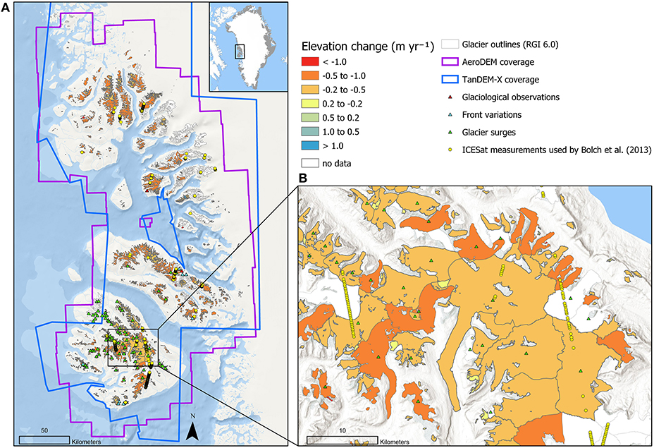
Figure 1. Glacier elevation changes in west-central Greenland. (A) The overview map shows the glacierized areas as based on RGI 6.0 together with elevation change rates from AeroDEM (1985) and TanDEM-X (2012) as well as ICESat tracks used by Bolch et al. (2013) and available information in the FoG database of the WGMS. (B) The inset map shows a close up of the study region located on Disko Island. This extract is subsequently used for close ups in Figures 2, 5 and Supplementary Figures 1, 3. Note that the points representing ICESat measurements (yellow points) are enlarged for visualization purposes and do not represent the actual footprint.

Digital Elevation Models

The AeroDEM (Korsgaard et al., 2016) represents the surface elevation in west-central Greenland in 1985, made from aerial photos acquired in July and August. It has a 25 m horizontal resolution, an accuracy of 10 m horizontally and 6 m vertically, assessed by co-registration to the ICESat data (Korsgaard et al., 2016). One challenge in using the AeroDEM arises from the use of optical images as source data for the DEM generation. They tend to have low contrast in snow-covered areas, especially in the accumulation areas of glaciers, or areas where no signal is captured from the surface due to clouds or shadows because of the viewing geometry (Korsgaard et al., 2016). Subsequently, they interpolated those areas resulting in partially strong artifacts in the DEM (i.e., rectangular features with improbable step-wise elevation changes of up to 60 m) (Supplementary Figure 1B). Following Korsgaard et al. (2016), we used the provided reliability mask to identify and remove those low quality areas resulting in data voids in the DEM. The reliability mask ranges from 0 to 100 differentiating between successful/good measurements (≥40), manually edited values or LIDAR points (22–39), and interpolated values (0–21). For elevation change assessments, Korsgaard et al. (2016) recommend filtering out values <40. After a plausibility check, we decided to also include areas with liability values 22–39 as we expect these areas to be of reasonable quality. These intermediate-valued pixels are distributed over the entire study area and cover ~200 km² of the glacierized area. Hence, areas with values <22 are claimed to be “low data quality” (Supplementary Figure 1C) and were therefore set to no data, resulting in data voids. By doing so, the AeroDEM covers ~53% of the total glacierized area and, hence, the remaining 47% are data voids. Visual inspection confirmed that with our approach, areas with strong artifacts have been removed (see Supplementary Figure 1C). We hereafter refer to the masked version of the AeroDEM as the AeroDEM for simplicity.

For this study we further used the recent high resolution TanDEM-X model for Greenland (Wessel et al., 2016) which was provided by the German Aerospace Center (DLR) for scientific studies. It originates from SAR X-band satellite imagery taken between December 2010 and July 2014 resulting in a mostly complete DEM with 12 m resolution. Hence, it represents the surface of the corresponding period based on weighted height averages of all data contributing to a scene. In our study region, 71 individual acquisitions (representing dates between 2010 and 2014) contributed to the final product. On the glacier basis, 3–15 acquisitions contribute to the surface of an individual glacier. Therefore, and as handled by Albedyll et al. (2018), we dated the TanDEM-X to 2012 ± 2 years and included the unknown difference in survey dates in the uncertainty assessment as described in the methods section. A bias is potentially introduced through the penetration of the X-band into snow and firn depending on the conditions of the surface layers. We discuss the potential influence of penetration biases on our results in the Discussion section Uncertainties and Bias. The comparison with ICESat elevation revealed good correspondence of the TanDEM-X at coastal regions whereas in inner parts the penetration can reach up to 10 m (Wessel et al., 2016). Supplementary Figure 1A shows the hillshade of the TanDEM-X of the same extent as for the AeroDEM.

Methods

The general workflow to calculate, amongst others, elevation and mass changes is shown in Supplementary Figure 2. The individual processing steps have been performed within a GIS and/or Python environment. Note that we calculated glacier changes for three different spatial levels: (1) individual glaciers (also called glacier-wide), (2) a glacier sample (consisting of the 1,526 glaciers with geodetic observations), and (3) the entire region of west-central Greenland (including the 1,526 glaciers with as well as the 859 without geodetic observations), as well as for entire Greenland periphery (including the 1,526 glaciers with as well as the 17,780 glaciers without geodetic observations).

Pre-processing

First, we re-projected all input data (AeroDEM, TanDEM-X, glacier outlines) to WGS 1984 UTM zone 22 N. After the removal of artifacts as described above, we re-sampled the TanDEM-X to the lower resolution of the AeroDEM (25 m) using bi-linear interpolation following Nuth and Kääb (2011). Subsequently, we co-registered the AeroDEM and the TanDEM-X following Nuth and Kääb (2011) using the TanDEM-X as the master DEM.

DEM Differencing and Outlier Filtering

By subtracting the AeroDEM from the TanDEM-X we calculated the difference DEM (dDEM) representing the change in surface elevation from 1985 to 2012 ± 2 years.

We next applied a filter to remove outlying elevation change values. However, several surging glaciers in this region locally produce very large elevation changes that are challenging for outlier statistics. Accordingly, we could not apply one global threshold to remove outliers (e.g., ±200 m) as this might also remove an actual signal. Therefore, we used an elevation-bin specific filter applied on a glacier-by-glacier basis: For each elevation bin, we calculated the mean and standard deviation of the elevation differences. Values that are more than three standard deviations from the mean were set to no data. Subsequently, the mean and standard deviation have been re-calculated, continuing until there were no more points to be filtered out (typically 2–3 iterations were necessary).

Void Filling and Calculation of Glacier-Wide Elevation Change

As we introduced data voids into the AeroDEM, they are obviously also present in the dDEM. The interpolation of voids in DEMs and dDEMs is a common procedure; however, the precise interpolation method is not standard. McNabb et al. (2019) assessed the impact and sensitivity of different void-filling methods on estimates of glacier volume change. Following the recommendations by McNabb et al. (2017), we chose to fill voids in the dDEM rather than in the original DEMs and, hence, selected five approaches to fill the voids in our dDEM. The subdivision “global” and “local” means that the mean/median was either calculated by considering the values of the entire region laying in the same elevation bin (i.e., “global”), or was calculated considering only values of the individual glacier (i.e., “local”). The five methods we have chosen are:

1. Linear interpolation of elevation differences (hereafter called linear),

2. mean elevation difference by elevation bin locally (hereafter called local mean),

3. median elevation difference by elevation bin locally (hereafter called local median),

4. mean elevation difference by elevation bin globally (hereafter called global mean), and,

5. median elevation difference by elevation bin globally (hereafter called global median).

The first method is the only method that used values from off-glacier pixels around the glacier outlines to linearly interpolate the voids inside the glacier outlines. All other methods exclusively considered areas within the glacier outlines. This is because we are assuming that the off-glacier changes are zero. For the linear interpolation [implemented using the griddata function provided as part of the SciPy python package (Jones et al., 2001)], it is reasonable to spatially interpolate from zero to the on-glacier value. For methods 2–3, the inclusion of off-ice pixels with (approximately) zero values would most likely depress the mean/median and so we excluded these data from our interpolation.

Methods 2–5 are so-called “hypsometric methods” building upon the assumption “that there is a relationship between elevation change and elevation” (e.g., McNabb et al., 2019). For this, we divided the dDEM in 100 m elevation bins (based on the TanDEM-X) and for each bin, we calculated the mean/median elevation change. Additionally, we applied a 2-fold void threshold for the hypsometric methods. The first threshold considered the fraction of voids per elevation bin: If an elevation bin had <40% coverage, the corresponding bin was rejected. If the entire glacier had <2/3 elevation range covered, the entire glacier was excluded from the sample. For the remaining glacier sample, we applied a second threshold considering the overall data coverage per glacier: If a glacier had <1/3 of its area covered by the dDEM, the glacier was excluded from the sample. For glaciers that were not excluded from the sample, we filled in any no-data bins using a third-order polynomial fit to the valid data.

Finally, based on the void-filled dDEMs and the glacier outlines, we calculated glacier-wide elevation changes as well as sample means for the entire observation period (1985–2012) and annually. So far, no multi-temporal glacier inventory is available for Greenland delineating the glaciers in the years the two DEMs reproduce the surface. Therefore, we used the outlines from RGI 6.0 representing the year 2001, which lays temporally between the DEMs and thus introduces a random error (cf. in the uncertainty assessment).

The specific elevation changes ($\Delta {\overline{h}}_i$) of the individual glacier in the unit m over the period of record (1985–2012) is simply the average glacier elevation change calculated from the difference between the AeroDEM and the TanDEM-X within the glacier outline. We calculated the sample average elevation change in two different ways:

(1) as the arithmetic mean:

$\begin{array}{ll}{\overline{\Delta h}}_{samplearithmetic}=\frac{\sum {\overline{\Delta h}}_i}{n}& (1)\end{array}$

(2) as the area-weighted average:

$\begin{array}{ll}{\overline{\Delta h}}_{samplearea-weighted}=\frac{\Delta V_{totarea}}{A_{sample}}=\frac{{\displaystyle {\sum }_{i=1}^n}{\overline{\Delta h}}_i·A_i}{A_{sample}}& (2)\end{array}$

where n is the number of glaciers (i.e., 1,526) and A_i is the area of the individual glaciers in 2001.

We calculated the sample mass change ΔM_tot (in the unit Gt)

$\begin{array}{ll}\Delta M_{tot}=\Delta V_{totarea}·\overline{\rho }& (3)\end{array}$

where $\overline{\rho }$ is a conversion factor assuming a density of 850 ± 60 kg m⁻³, following Huss (2013). Hence, the sample mass change is based on the area-weighted average elevation change. We calculated regional mass changes analogously using A_region instead of A_sample.

For the annual elevation and mass-change rates we divided ${\overline{\Delta h}}_i$, ${\overline{\Delta h}}_{samplearithmetic}$, ${\overline{\Delta h}}_{samplearea-weighted}$ and ΔM_tot by the number of years between the two DEMs (i.e., 27 years).

Uncertainty Assessment

For the uncertainty assessment we followed Zemp et al. (2019) and extended their calculations using additional terms to account for the uncertainties introduced by the void-filling approach (σ_{void fill}), and the fuzzy date of TanDEM-X (σ_{TDX date}). We assumed all errors are uncorrelated and random. Supplementary Figure 2 indicates from which input data or processing step the individual error components originated.

For an Individual Glacier

As the individual errors for the uncertainty of the glacier-wide specific elevation change (σ_Δh) are independent, we calculated it based on the following formula:

$\begin{array}{ll}{\sigma }_{\Delta h}=\sqrt{{{\sigma }_{DEM}}^2+{{\sigma }_{voidfill}}^2+{{\sigma }_{TDXdate}}^2}& (4)\end{array}$

For the uncertainty of the mass change (σ_ΔM), we had to consider the uncertainties of the glacier-wide specific elevation change (σ_Δh), the uncertainty in the density assumption (σ_ρ) as well as the error of the glacier area (σ_area) and was calculated as follows:

$\begin{array}{ll}{\sigma }_{\Delta M}=|\Delta M|·\sqrt{{\left(\frac{{\sigma }_{\Delta h}}{\overline{\Delta h}}\right)}^2+{\left(\frac{{\sigma }_{\overline{\rho }}}{\overline{\rho }}\right)}^2+{\left(\frac{{\sigma }_{area}}{\overline{A_{sample}}}\right)}^2}& (5)\end{array}$

Individual Error Components

For each glacier, we estimated the error in the variable σ_DEM following McNabb et al. (2019) based on the equation:

$\begin{array}{ll}{\sigma }_{DEM}=\sqrt{{({\sigma }_{\Delta z}A)}^2+{({\sigma }_{area}\Delta z)}^2}& (6)\end{array}$

where σ_Δz was estimated based on the mean off-glacier difference between the two DEMs after co-registration and the residual differences after co-registration to ICESat (i.e., the triangulation procedure described in Paul et al., 2017), A is the glacier area, σ_area is the error in glacier area, here equal to 0.1 in order to conservatively consider the uncertainty for the glacier areas which is 5% (or 0.05) according to Rastner et al. (2012), and Δz is the mean elevation difference of on-glacier pixels.

The uncertainty introduced by the void-filing approach (σ_{void fill}) we estimated for each glacier as 1.96 standard deviations of the elevation changes resulting from the two void-filling methods considered to produce reasonable results (i.e., local mean and local median, cf. discussion). By doing so, we implicitly consider the fraction of data voids, as the error is potentially larger for glaciers with a larger fraction of voids.

The date uncertainty of the TanDEM-X (σ_{TDX date}) we estimated to be ± 2 times the annual elevation change rate from 1985 to 2012. Note that it does not consider the influence of seasonal variations, however it is (most likely) minimized as the period of record is more than 20 years.

The uncertainty for the volume-to-mass conversion ${\sigma }_{\overline{\rho }}$ was set to ± 60 kg m⁻³ based on Huss (2013).

For the uncertainty in the glacier area (σ_area) we again refer to the study of Rastner et al. (2012) that reported a mean area uncertainty of 5% for the glacier outlines used here. Further, the absence of outlines around the time of the DEMs introduced an additional uncertainty due to two compensatory effects: Distinct negative elevation changes right in front of the glacier tongue imply that this area actually was glacierized before 2001 and should be included (e.g., visible for the glacier in the lower left corner in Supplementary Figure 3). Hence, the estimated on-glacier averages are too positive, since the areas excluded tend to have more negative elevation changes overall (i.e., estimated elevation change is slightly too positive). This effect is balanced by the fact that the area we are using is too small as the outlines represent the area after the mid-period between 1985 and 2012 (i.e., estimated elevation change is slightly too negative). The latter could be adjusted by the application of an area change rate but this was not required here as those effects matter only for time series. Nevertheless, we applied a conservative uncertainty in the area by doubling the uncertainty given by Rastner et al. (2012) to account for this effect, too.

Composite Sample Errors

These calculations above have been done for individual glacier outlines (i.e., for each of the 1,526 glaciers). To assign uncertainties to the sample average (as in Table 2), we calculated the uncertainty of the sample-wide elevation change (σ_{Δh sample}, for the arithmetic mean and the area-weighted average) as well as of the sample-wide mass change (σ_{ΔM sample}) as:

$\begin{array}{llll}{\sigma }_{\Delta Msample}& =& \sqrt{{\displaystyle \sum _{i=1}^n}{\sigma }_{\Delta M,i}^2}& (7)\end{array}$

$\begin{array}{llll}{\sigma }_{\Delta hsamplearithmetic}& =& \frac{\sqrt{{\displaystyle {\sum }_{i=1}^n}{{\sigma }_{\Delta h,i}}^2}}{n}& (8)\end{array}$

$\begin{array}{llll}{\sigma }_{\Delta hsamplearea-weighted}& =& \frac{{\sigma }_{\Delta Msample}}{\overline{\rho }·A_{sample}}& (9)\end{array}$

Results

Pre-processing, DEM Differencing, and Void Filling

Before the co-registration the shift on stable terrain between the AeroDEM and TanDEM-X was 6.1/−12.3/−0.9 m in x/y/z directions. After the co-registration, these values have been reduced to 0.7/0.5/−0.1 m with a mean vertical offset of 0.1 m, which is considered in the uncertainty analysis.

Supplementary Figure 3 shows the result of the subtraction of the TanDEM-X from the AeroDEM for glacierized as well as for the surrounding areas. White areas are data voids resulting from the previously generated data voids in the AeroDEM. Several glaciers, for instance the glacier in the middle of the image, clearly show the pattern of surging activity between geodetic survey dates (rising surface at the tongue, surface lowering in the accumulation area).

Figure 2 shows the dDEMs for the glacierized areas resulting from application of the five different void-filling methods. Note that for the four hypsometric methods, some glaciers do not have elevation change information as the data void threshold process described above has filtered them out. Comparing the results, several differences are visible among the approaches which are also described by McNabb et al. (2019):

1. The hypsometric methods (Figures 2B–E) smooth the elevation change pattern, whereas the linear method preserves the pattern that is already existent in the non-filled dDEM.

2. The local hypsometric methods produce discontinuities at the lines dividing neighboring glaciers, as the calculations are glacier-wide. Especially for ice caps, such disruptive changes are not very plausible for neighboring glaciers.

3. The global methods do not appropriately reproduce the elevation change pattern of some individual glaciers, as is clearly visible for the surging glaciers.

FIGURE 2

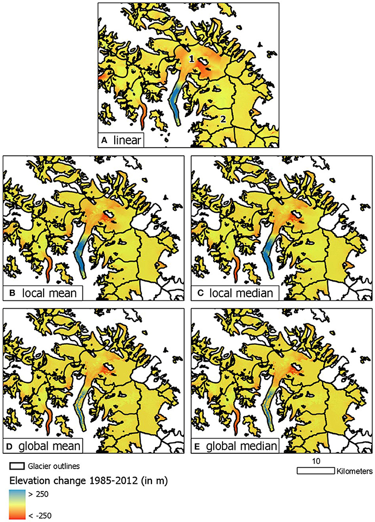
Figure 2. Visual comparison of the DEM differencing resulting from the various void-interpolation methods: (A) linear interpolation of elevation differences, (B) mean elevation difference by elevation bin locally, (C) median elevation difference by elevation bin locally, (D) mean elevation difference by elevation bin globally, (E) median elevation difference by elevation bin globally. In general, the glaciers show elevation losses with higher losses at the tongues whereas the large surging glacier in the middle shows a reversed pattern (elevation gain at the tongue, elevation loss higher up). Note how the different void-interpolation methods influence the elevation change pattern. For instance, the global methods do no generate appropriate results for the surging glacier. In case a glacier had a large fraction of voids, no elevation changes have been calculated (white glaciers, cf. methods). Glaciers 1 and 2 in (A) refer to the results in Table 1.

Table 1 compares the average sample elevation change values for the entire observation period resulting from the different interpolation methods for the entire region as well as for two individual glaciers which have ~60% data voids in the dDEM: one surging glacier (1) and one non-surging glacier (2). The results summarized in Table 1 show that for the sample average the different methods produce similar values. However, for glacier-wide calculations, mainly for surging glaciers, the values can vary significantly: the linear and global methods give very high glacier-wide elevation change values, whereas the local median method gives very low values. In general, for regional assessments, the differences among the methods are not significant but for glacier-wide assessments, the method selection appears crucial, as some methods are unable to reproduce the pattern among differently behaving glaciers, such as surging vs. non-surging glaciers.

TABLE 1

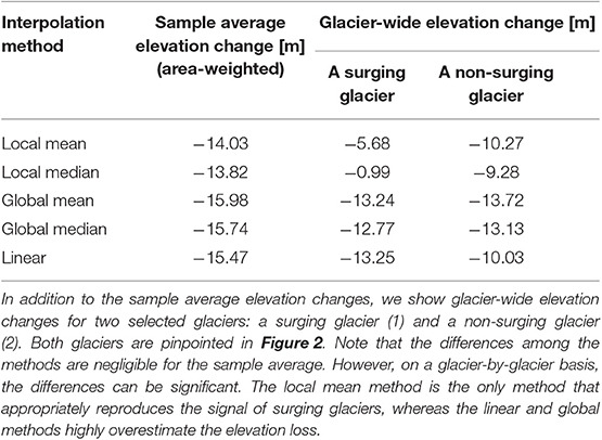
Table 1. Comparison of glacier elevation changes of the 1,526 glaciers in west-central Greenland from 1985 to 2012 based on different void-interpolation method.

For this study, we used the local mean (per elevation bin) method as our best guess to fill the voids in the dDEM of our study region. This choice is recommended by our results, by the findings in McNabb et al. (2019), by the distribution of voids in the data, and by the characteristics of the glaciers in this region as it better accounts for the characteristics of individual glaciers when compared to the other methods (cf. discussion). However, this remains a best guess, as the true elevation changes across the data gaps are unknown. Nevertheless, the following results are based on the application of the local mean method to interpolate missing elevation change values.

Glacier Elevation and Mass Changes

The 2-fold data void threshold applied to the hypsometric methods caused the exclusion of ~850 glaciers. Accordingly, our approach made it possible to calculate glacier-wide elevation changes for 1,526 glaciers covering approximately two third of the total number and 68% (3,785 km²) of the total glacierized area of west-central Greenland (Figure 1A). Figure 3A shows the hypsometry, the corresponding annual elevation change per elevation bin, and the annual volumetric change per elevation bin for the entire glacier sample. Figures 3B–E show the same for four subsamples, which are further analyzed in the discussion. The data voids that have been interpolated (red bars) are mainly in the accumulation area and make up ~37% of the area. The gray bars indicate the hypsometry for all the 2,385 glaciers located in west-central Greenland.

FIGURE 3

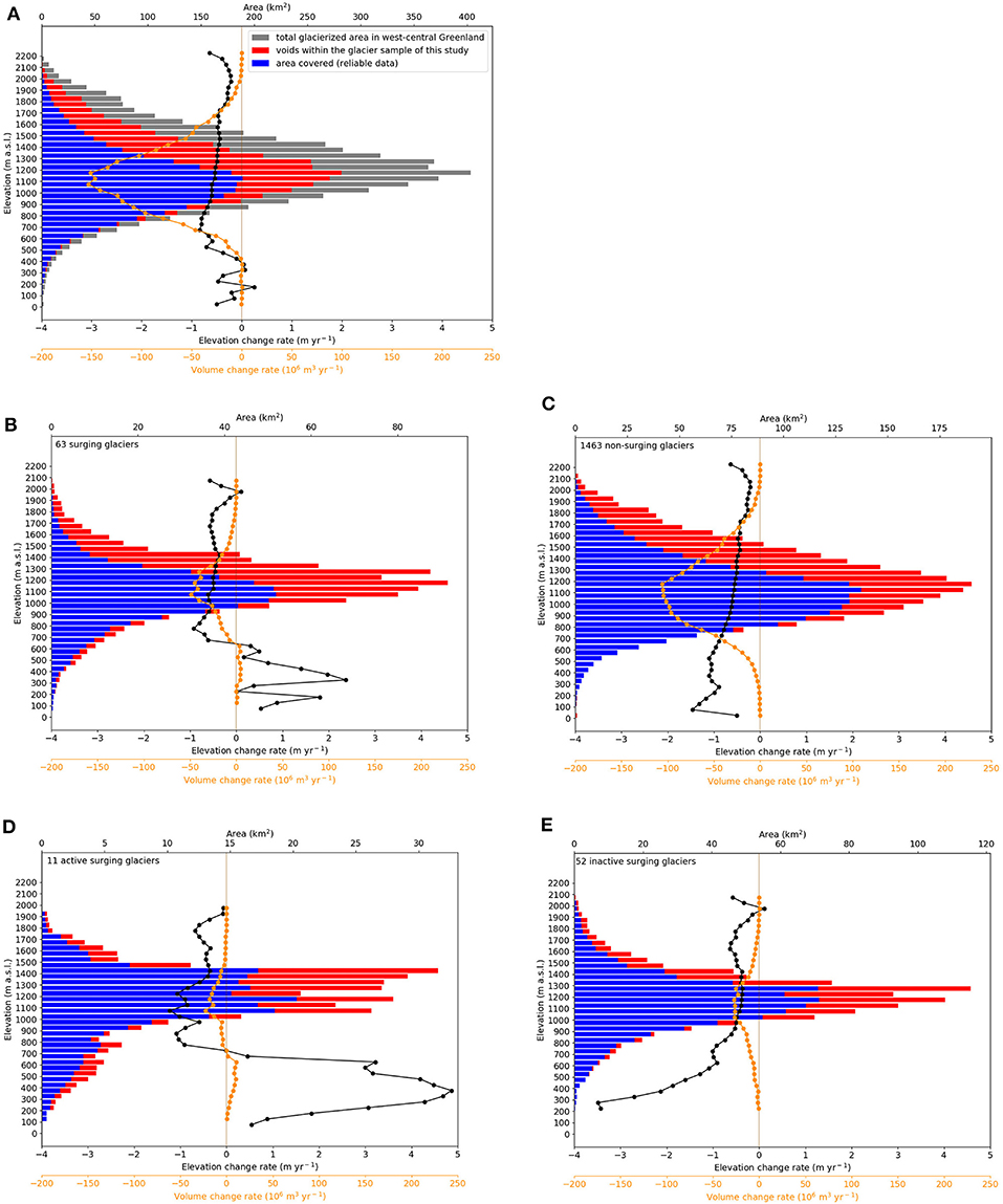
Figure 3. Hypsometric glacier changes in west-central Greenland between 1985 and 2012. (A) The plot in the first row shows the glacier distribution with elevation (y-axis) for all glaciers in the region (gray) as well as for the investigated glacier sample with geodetic observations (blue) and original data voids (red). The average elevation and volumetric changes per elevation bin are shown as black and oranges lines, respectively, with corresponding y-axes. The second row shows the same plot but dividing the sample into glaciers with (B) and without (C) reported surge activities. In the third row, the surge glaciers (B) are divided into active (D) and inactive (E) subsamples based on corresponding indications in the elevation change fields.

Regarding surges, 63 of the 1,526 glaciers, almost all of them located on Disko Island, show evidence of surging activity: Based on the dataset of Sevestre and Benn (2015), for 52 of these glaciers surging activity is “probable” and for four of these glaciers surging activity has been observed. Based on our dDEM, we flagged seven additional glaciers as surging glaciers (cf. discussion). Three glaciers are labeled as marine terminating glaciers in the RGI. However, based on a visual inspection of RapidEye data, two of these glaciers do not appear to reach the sea any more, and hence, we do not discuss these glacier-types here.

Additionally, we want to point out the reduced elevation changes in the lowest elevation bin visible in Figure 3C and slightly visible in Figure 3E. This might be explained through the lack of a second glacier inventory coincident with the TanDEM-X. That is, we include areas that became deglaciated between 2001 and 2012 and hence there is no more potential ice present to cause negative elevation changes. As a result, the mean elevation changes per bin can be less negative. However, this fraction compared to the overall glacier area is small and considered in the uncertainties.

Table 2 summarizes the average elevation and mass change (in m, Gt, and SLE) of our sample for the entire observation period as well as annually. Regarding the elevation change, there are slight differences between the arithmetic and the area-weighted mean showing that a few large glaciers have more negative elevation changes. We considered the latter to be most appropriate for regional mass-change assessments and was therefore used for further calculations. Hence, the observed glacier sample on west-central Greenland lost ~14.0 ± 4.6 m of ice thickness from 1985 to 2012 or 0.5 ± 0.2 m yr⁻¹, respectively. This is equivalent to a total mass change of −45.1 ± 14.9 Gt (−1.7 ± 0.6 Gt yr⁻¹), or 0.13 mm SLE, assuming an ice density of 850 ± 60 kg m⁻³. Further, comparing the signal (−14 m) and the bias identified by the co-registration shows the relevance of the latter: without the co-registration there would be a bias of ~6% of the actual signal.

TABLE 2

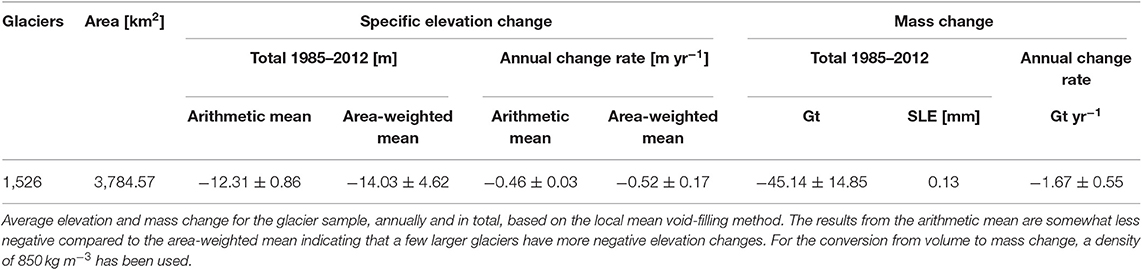
Table 2. Elevation and mass changes of the observed glacier sample in west-central Greenland between 1985 and 2012.

Discussion

Void-Filling Methods

The handling of data voids for elevation-change assessments is neither straight forward nor does a commonly used and established method yet exist. The different methods described in the literature can have different effects on the resulting estimates (McNabb et al., 2019). The major challenge arises from the ignorance about the true elevation changes across the data gaps. Therefore, McNabb et al. (2019) artificially produced data voids in DEMs over southeast Alaska to identify which method reproduces the reality most accurate. However, the best-performing method in that study (linear interpolation of voids in the dDEM) cannot just be transferred to any other region with data voids in the DEMs. Three conditions majorly influence the identification of the appropriate void-filling method: (a) the aim of the study: calculation of region-wide vs. glacier-wide elevation changes, (b) the characteristics of the glaciers in the study area (e.g., surging glaciers), and (c) the distribution of the data voids which is not expected to be the same for each region, or even each DEM. Given the circumstances for this study of glaciers in west-central Greenland [(a) aiming for glacier-wide elevation changes, (b) the presence of surging glaciers, and (c) voids mainly in accumulation area], we chose five methods recommended by McNabb et al. (2019) to identify the influence on the estimates for our study region. Additionally, this multi-method approach allowed an uncertainty assessment of the void-filling method (see Methods). Our results indicate that for these circumstances, the global methods are inappropriate for glacier-wide elevation change assessments. Additionally, the linear method is not appropriate considering that the resulting dDEM has a frequently noisy dhdt signal. Nevertheless, these methods produce reasonable results for regional assessments.

Hence, for our study we used (a) a local method because surge glaciers are abundant in our region and (b) we used a hypsometric method because of the elevation-dependency of the signal (at least for non-surging glacier, cf. Figure 3). Of the remaining methods, it was difficult to identify the one method performing best, as we do not know the true values. However, as in McNabb et al. (2019) the (artificial) voids also prevail in the accumulation area, we followed their recommendations and agreed that the local mean method potentially reflects the change of the individual glaciers appropriately as it includes the area-elevation distribution of each individual glacier.

The threshold applied to reject glaciers based on the fraction of data voids can influence the sample size as well as the results. For regional glacier mass balances, such a threshold is usually and justifiably not applied and all the data available is considered for the corresponding study region. For glacier-wide studies, such a threshold is either most often not applied, the fraction of data voids is not declared, or the handling of data voids is not clear. Otherwise, different void thresholds on a glacier-wide basis are applied to exclude glaciers, such as 30% (e.g., Brun et al., 2017) or 20% voids (e.g., Le Bris and Paul, 2015). Hence, there is no consensus as to how much of the area of a glacier should be covered by data in order to be considered. Due to the partly large fraction of data voids in the DEM used here, a void threshold of 30% would have substantially reduced our sample to ~600 glaciers. Therefore, we used a 2-fold threshold: As it considers the minimal area covered in combination with a minimal fraction of the hypsometry covered, we ensured to get a glacier sample that is optimally covered with data. Nevertheless, based on the aim of the study and the end user, a modification of this threshold might be reasonable. For regional estimates, the thresholds (for exclusion) can be set relatively low to increase the sample size. However, for analyses interested in individual glaciers, these thresholds need to be set in a much more rigorous way. This study tries to combine both: a statistically representative sample (about two third coverage) for regional mass-change estimates with plausible glacier-wide results (for submission to the WGMS).

Uncertainties and Bias

The total error related to the elevation changes of our sample is a composite of three different error sources: DEM, void-filling, and date. The former two errors vary widely among the individual glaciers and account for the largest contribution. The error related to the date uncertainty contributes only minimally due to the long observation period. However, its consideration is important as it contributes more with decreasing observation length and increasing rate of elevation change.

The application of TanDEM-X data introduces a bias caused by the penetration of the radar signal into snow. However, the magnitude of this effect depends strongly on snow and firn conditions and, hence, can vary considerably (Lambrecht et al., 2018).

In the following, we illustrate, using our data, how the results could be corrected to account for the radar penetration in cases where the observation period is shorter and hence the penetration has a significant effect on the results. We can estimate signal penetration similar to previous studies (e.g., Malz et al., 2018; Braun et al., 2019): The radar penetration takes place only in the accumulation area (assumed AAR of 50%) and is between 0 m (at ELA) to 5 m at the summit. On average (over the elevation range of the accumulation zone), this makes 2.5 m with an uncertainty of 2.5 m. Averaged over the entire glacier, then, this is halved again to 1.25 ± 1.25 m (because only the accumulation area, which covers about half of the glacier, will be affected by radar penetration). Obviously, this correction introduces another uncertainty related to whether a glacier is actually affected by the radar penetration. Hence, this has to be considered in the uncertainties by adding the factor σ_{radar penetration} to the uncertainty assessment, which we propose to be as high as the correction factor itself (1.25 m). Due to the long period of records (27 years), the strong signal (−14 m), the relatively large uncertainty (±4.6 m), and due to the fact that the TanDEM-X is a stacked product using acquisitions over multiple seasons and years making a coherent radar penetration unlikely, the bias and related uncertainty of a potential radar penetration could be ignored in our study. Hence, we did not correct our results by an estimated correction value also because such a correction might result in a disimprovement. Nevertheless, for shorter observations periods and if the TanDEM-X represents only winter acquisitions which would favor significant radar penetration, a correction is strongly advised.

Influence of Surge Type Glaciers on Elevation Changes

Surging glaciers display a distinct dynamic behavior (e.g., Hewitt, 2007; Gardelle et al., 2013; Rankl et al., 2014; Paul, 2015). Typically during a surge, a large amount of ice in a reservoir further upglacier is transported downwards, where it is then more prone to ablation (Paul, 2015). If this happens between two points in time represented by DEMs, the process becomes apparent when subtracting the two DEMs (i.e., negative elevation changes will be observed in the accumulation area, positive changes in the ablation area; e.g., the large glacier in Figure 2). Hence, they show the opposite pattern to glaciers reacting to current climate change (negative elevation changes at the tongues, no/slight positive elevation changes in the accumulation area). In the case of west-central Greenland, 63 glaciers were marked as glaciers with (evidence for) surging activity. However, we identified this switched pattern in our dDEM for only 11 glaciers. Hereafter we name these glaciers “active surging glaciers” for our observation period and the remaining 52 glaciers previously identified as surging glaciers are named “inactive surging glaciers.” Figure 3A shows the glacier hypsometry, the mean elevation change per bin as well as the volumetric change per bin for the entire glacier sample. Figures 3B–E show the same but for the 63 glaciers with evidence for surging activity, the 11 active surging glaciers, the 52 inactive surging glaciers and the 1,463 non-surging glaciers, respectively. In terms of elevation change per elevation bin, the 63 surging glaciers partly show the expected switched pattern which is very pronounced for the 11 active surging glaciers. Interestingly, the strong positive elevation change at the tongues from the 11 active surging glaciers dominates the lowest bins of the 1,526 glaciers, as the pattern is apparent in the elevation changes, too. The 52 inactive surging glaciers show pronounced negative elevation changes at the tongues. However, this pattern is induced by approximately seven glaciers that are in this state of post-surge recovery (i.e., strong ablation at the tongue and pronounced accumulation further up). This is typical for glaciers after a surge as the mass transported further down is now prone to melting (Paul, 2015). The rest of the inactive surging glaciers as well as the non-surging glaciers show the typical negative elevation changes at low elevations that decrease with increasing elevation. All figures, especially Figures 3A,C, show that in terms of volumetric balance the mid-elevations with the highest fraction of area majorly contribute to the volume change. Whereas, the contributions from the lowest (i.e., glacier tongues) and highest areas are nearly negligible due to the small area, and hence, so is the influence of surging glaciers on the volume change per bin. Consequently, an exclusion of the 63 glaciers with evidence for surging does not affect the sample average (hypsometry-weighted) elevation change.

Comparison With ICESat Based Studies

Here we focus on the comparison of the elevation changes for our sample with the ones estimated by Bolch et al. (2013) and Gardner et al. (2013). Their studies are pioneering, as they are currently the only studies that have determined the mass change of Greenland's peripheral glaciers including the glaciers in our study region. Hence, the comparison with their work is fundamental.

Bolch et al. (2013) applied ICESat data from October 2003 to March 2008 and also used the glacier inventory from Rastner et al. (2012) but an older version (RGI 2.0). In their study the west-central sector covers 5,045 km² (521 km² less than the west-central sector in this study) as it spreads about 65 km less toward north. They calculated an average elevation change rate for the west-central sector of −0.28 m yr⁻¹ for the period 2003–2008 by simply averaging the elevation change values of 285 ICESat measurements laying on 47 glaciers (CL0-1) in west-central Greenland. Their result is about half of the change rate as calculated for the sample of this study covering the period 1985–2012 (−0.52 m yr⁻¹). As the processed ICESat footprints of their study are available for comparison, we further discuss these differences between the elevation changes in the following.

First, it has to be noted that we are comparing different time periods, hence a period of enhanced mass loss before 2003 relative to the time period after would explain our more negative values. However, we found no indication of a more negative mass-balance period before 2003, in fact rather the opposite. The negative glacier length changes on Greenland, in the late twentieth century (Leclercq et al., 2014) reject this hypothesis. In addition, Zemp et al. (2019) combine our dDEM results with the temporal variability from glaciological observations [i.e., from Freya (E-GL), Mittivakkat (E-GL), Qasigiannguit (SW-GL), Storglaciären (SE), Storbreen (NO), White (CA)] indicating that recent mass changes in Polar Regions are at least as negative as since the 1980s.

Regarding the coverage of the applied ICESat measurements, we want to highlight that the 285 footprints of 70 m cover an area of ~1.1 km². Hence, they cover only about 0.03% of the area of west-central Greenland that we cover in this study. Further, the distribution of the ICESat measurements applied by Bolch et al. (2013) on the glaciers in the study region (Figure 1B) shows that they are mainly located in the accumulation area. However, the missing representation of the glacier tongues is probably not sufficient to explain the differences, given the large number of surging glaciers observed in the region, which pose a major challenge for elevation change assessments using ICESat data. Therefore, we compare their results with our results in more detail.

The 285 ICESat measurements used by Bolch et al. (2013) cover 47 glaciers in west-central Greenland, of which 27 glaciers representing an area of 604 km² (and 136 ICESat measurements covering 0.5 km²) overlap with the 1,526 glaciers considered in this study. Comparing those 27 glaciers with our 1,526 glaciers regarding the latitudinal distribution and the variety of glacier size, indicates that the sample of Bolch et al. (2013) reasonably well represents our glacier sample. Their sample slightly underrepresents low- and high-lying glaciers (none of the 27 glaciers has a median elevation below 700 and above 1,600 m a.s.l). Nevertheless, the limited representation of the ICESat measurements due to their small footprint is undisputable as shown in Figure 4. It shows the hypsometries of the 1,526 glaciers covered in this study, for the 27 glaciers covered in both studies, and for the 136 ICESat measurements. However, the latter is only visible by considerably zooming in on the former hypsometries due to the very little area coverage by the ICESat measurements (Figure 4, inset). Nevertheless, limited coverage does not necessarily mean the result is less correct. It depends on whether the subsample is representative for the population. Bolch et al. (2013) cover the elevations where most of the glacierized areas are located and majorly contribute to the volume changes as seen in Figure 3. The question is now, whether these few elevation-change measurements are representative for the full glacier sample. Figure 4 also shows the elevation changes per elevation bin for the 1,526 glaciers of this study (black), for the 136 ICESat measurements (yellow) and the 136 measurements extracted from our dDEM at the ICESat locations (blue). We extracted the point values from our filled dDEM using cubic interpolation of the dDEM values surrounding the footprint center. Figure 4 shows a pronounced variation of the ICESat measurements among the elevation bins as well as two outliers with strong positive values for bins where the coverage of the ICESat data is exceptionally low (750 and 1,500 m a.s.l.). This indicates that these measurements are rather accidental and not representative for the corresponding elevation bin. Hence, such values are highly sensitive for the calculation of the average elevation change by simple averaging, especially if the coverage is limited.

FIGURE 4

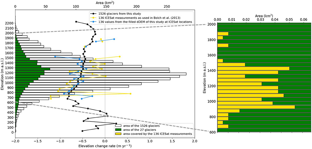
Figure 4. Comparison of hypsometric elevation change rates between the present study and ICESat estimates from Bolch et al. (2013). The average elevation changes per elevation bin from this study, from the 136 ICESat estimates and from the 136 values from our change field at the ICESat locations are shown as black, yellow and blue lines, respectively. The bars represent the glacierized area with elevation covered by the 1,526 glaciers of this study (white), by the 27 glaciers that overlap between this study and the study of Bolch et al. (2013) (green), and by the 136 ICESat measurements (yellow). The latter is only visible when considerably zooming in as shown in the inset on the right (note the different scales for area).

The comparison of different averaging methods can identify whether an averaging method that is less prone to outliers leads to more accurate elevation change values (assuming our results with full observational coverage as reference). To do so, we compare the annual elevation change-rates for 136 locations based on (a) the dDEM calculated in this study (hereafter called 136 dDEM measurements) and (b) the ICESat measurements as used in Bolch et al. (2013) (still called 136 ICESat measurements). We averaged the 136 values, either from the dDEM or from the ICESat measurement, by four methods: (1) by the arithmetic mean of all points, (2) by the arithmetic mean of the 27 glacier-wide mean values, (3) by the area-weighted mean of the glacier-wide mean values, and (4) by the hypsometry-weighted mean. For the latter, we averaged the elevation changes for each elevation bin (over all 27 glaciers), multiplied this value with the area of the corresponding bin and divided the sum by the total area of the 27 glaciers. Method (1) was used by Bolch et al. (2013) to calculate the regional elevation change based on their entire sample (285 ICESat points). We averaged the elevation changes for each elevation bin, multiplied this value with the area of the corresponding bin and again divided the sum by the total area of the 27 glaciers. As we applied each of the four methods to the 136 dDEM and 136 ICESat measurements, we end up with eight different results. An additional result is given, referred to as the reference, by calculating the area weighted mean based on the entire dDEM for the 27 glaciers. Figure 5 illustrates the calculations using the extract on Disko Island and gives the corresponding results for all 27 glaciers and 136 measurements, respectively. The two columns indicate which dataset has been used (our dDEM or the ICESat measurements), (a) gives the reference result (−0.48 m yr⁻¹) referring to the area-weighted mean elevation change-rate for the 27 glaciers based on the entire dDEM of this study. This value is similar to the elevation change calculated for our entire sample of 1,526 glaciers (−0.52 m yr⁻¹) indicating that these 27 glaciers are an appropriate representation of the 1,526 glaciers in terms of elevation change. Figures 5b–i show the change rates based on the four different averaging methods, as based on the 136 dDEM for the period 1985–2012 and based on the 136 ICESat data for the period 2003–2009.

FIGURE 5

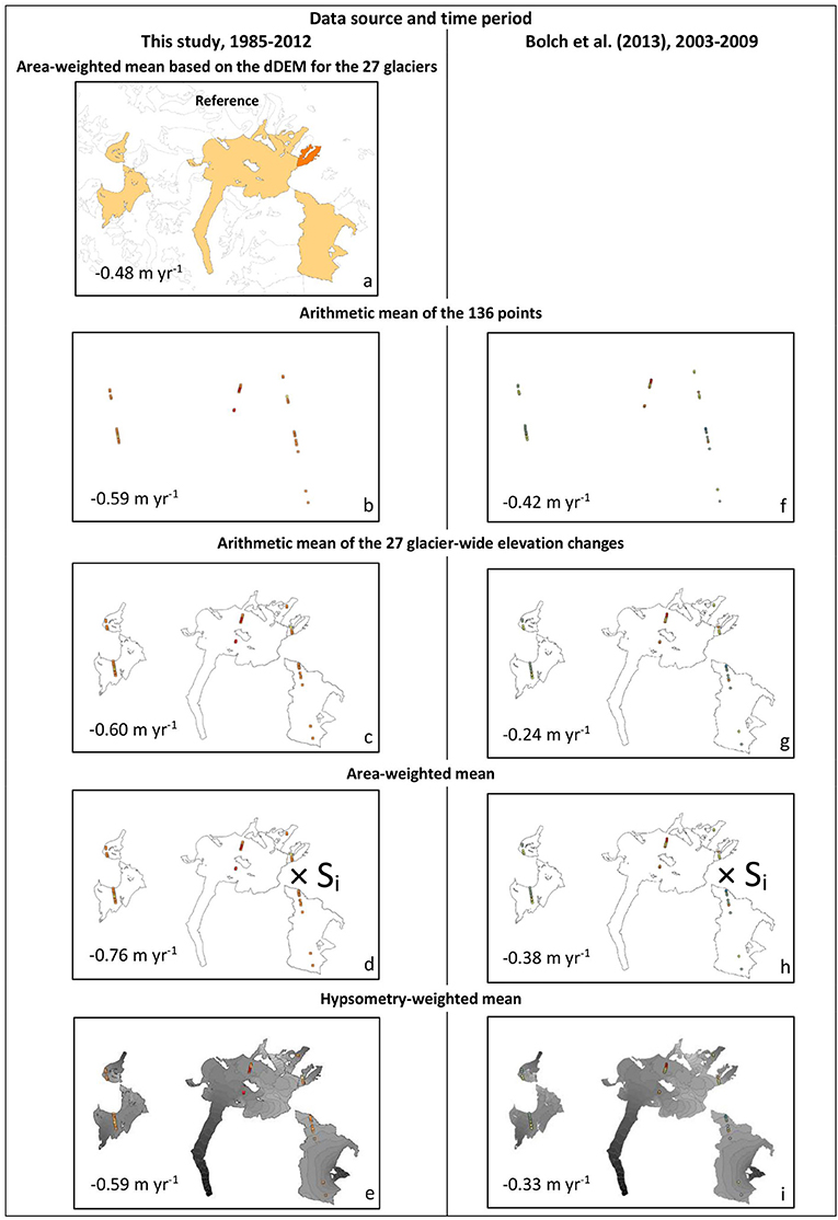
Figure 5. Illustration and corresponding results of the different averaging methods (rows) to calculated the mean elevation change for the 27 glaciers based on (a–e) measurements from this study at 136 ICESat locations and (f–i) 136 ICESat measurements used by Bolch et al. (2013). See text for calculations. Note that the points and squares representing dhdt measurement locations do not represent the actual area of the 70 m footprints.

From these results, we can deduce two main findings: (1) Applying the four methods to the 136 dDEM measurements (b-e) shows that the ICESat footprint has a negative bias with respect to the reference result. However, this does not help to explain the difference between our result and Bolch et al. (2013). In fact, the difference would increase when applying such a bias-correction. (2) The ICESat column (f–i) shows that the ICESat observations seem to be less equally distributed with respect to glaciers and elevations bins and hence are more sensitive to the averaging method. Thus, the ICESat results seem to have a stronger variability and feature a different elevation change pattern as compared to our dDEM. In conclusion, the ICESat coverage is too small and very sensitive to the averaging method. Therefore, the sample is not representative for estimating the regional glacier changes.

Moreover, we would expect that the results from the arithmetic mean of the 136 ICESat measurements (f) are less negative than of the 136 dDEM measurements (b). Zemp et al. (2019) show that the annual mass change in Greenland increased significantly from the 1980s until 2016. Hence, the ICESat measurements should be more negative than the dDEM values. However, the results show the opposite is true. Besides the limited, non-representative coverage being the cause for this, an additional issue might add to the underestimation of the elevation changes. We assume a regression issue exists in the ICESat data used by Bolch et al. (2013): For the regression procedure to determine the elevation changes, they used ICESat data from October 2003 to March 2008. Hence, their observations start at the end of the ablation season but terminate at about the time of highest (winter) accumulation. This might cause the regression to be less negative, as it would be using data from a low point (late summer) as the end point for the regression. An additional indication for this effect can also be seen in Figure 4: for 13 out of 21 elevation bins, the ICESat measurements are less negative than the dDEM values.

Gardner et al. (2013) also determined the average elevation and volume change for, amongst others, west-central Greenland based on ICESat data. They applied methods comparable to the ones from Bolch et al. (2013), however, based on their publication we came across two main differences: First, they used data between October 2003 and October 2009, hence the regression issue does not arise. Second, their selection of ICESat measurement sample is different and larger. This potentially explains why they calculate an elevation change for west-central Greenland of −0.51 ± 0.26 (95% CI) m yr⁻¹, which is consistent with our estimates.

Overall, the comparisons above show that a coverage issue in ICESat measurements does not necessarily result in inaccurate results (as shown by the results in Gardner et al., 2013). However, the selection of the ICESat points is crucial: If data are sparse, the result can be much more vulnerable to inappropriate representativeness of the point measurements for the entire glacierized area. Additionally, the selection of the start and end point for regression analysis in short observation periods (<10 years) might be crucial as it potentially influences the annual change rate.

Mass Change and Its Extrapolation to Unmeasured Regions

Based on the average elevation change of the 1,526 glaciers, we calculated the specific mass change for these glaciers by applying a density assumption of 850 ± 60 kg m⁻³ (Huss, 2013). We calculated the total mass change of the region by multiplying the mean specific mass change of our sample by the area of the entire glacierized region (i.e., entire west-central Greenland and entire Greenland periphery). Table 3 illustrates the resulting mass changes for all 2,385 glaciers in west-central Greenland, for all of west-central Greenland as defined by Bolch et al. (2013), as well as for all peripheral glaciers on Greenland. Additionally, for west-central Greenland and the whole of Greenland periphery the estimates from Bolch et al. (2013) and Gardner et al. (2013) are given for their corresponding time period. The difference in the annual mass change rates estimated here, and the estimates of Bolch et al. (2013), are mainly caused by the strong differences in the elevation change estimates, and to some degree by their lower ice density assumption. Our study suggests annual mass loss rates (−2.23 Gt yr⁻¹) about twice as large for the same extent of west-central Greenland. We point out that the extrapolation of our estimates to entire peripheral Greenland (−40 Gt yr⁻¹) might be associated with large uncertainties, provides only a rough estimate and serves for an order of magnitude comparison with existing studies. In general, the average annual mass loss of west-central Greenland is somewhat lower than the average loss for the rest of Greenland periphery (Bolch et al., 2013). Hence, our extrapolated values might even underestimate the Greenland-wide overall mass change. Accordingly, based on our estimates we determined an annual mass loss for the entire Greenland periphery of 40 Gt yr⁻¹ for 1985–2012 which is ~30% more than estimated by Bolch et al. (2013). However, our values correspond to the estimate provided by Gardner et al. (2013) of an annual mass loss for the whole of peripheral Greenland of 38 ± 7 Gt, even though they applied different density assumptions for the accumulation and ablation area, and not a constant value as we did.

TABLE 3

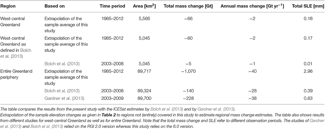
Table 3. Regional glacier mass changes for Greenland.

Conclusions

This study presents for the first time glacier-wide elevation changes for a large sample of Greenland's peripheral glaciers. We assessed geodetic balances for 1,526 glaciers in west-central Greenland from 1985 to 2012 based on the recently released AeroDEM and TanDEM-X. These two DEMs offer great opportunities for geodetic elevation change assessments but also introduce various challenges, such as artifacts or data voids in the AeroDEM or radar penetration and the imprecise date of the TanDEM-X data. For the handling of artifacts and data voids, various methods exist, each of which have a different effect on the resulting elevation change values. Hence, the selection of an appropriate method is not straightforward and no general procedure can be given, as this strongly depends on the research questions, the distribution of the data voids, and the glacier characteristics of the study area. Given these criteria, we found the local mean hypsometric method to be suitable for west-central Greenland where surge-type glaciers are abundant. The uncertainty introduced by the imprecise date of the TanDEM-X is reflected in our uncertainty analysis. We discussed how any potential radar penetration can be taken into account, however we refrained from a corresponding correction in this study as the potential bias and related uncertainties are negligible in view of the length of the time period, the overall glacier change rates, and the overall uncertainties.

Our results show that the glaciers in west-central Greenland have lost ~14.0 ± 4.6 m of ice from 1985 to 2012 or −0.5 ± 0.2 m yr⁻¹, respectively. This is equivalent to a total mass change of −45.1 ± 14.9 Gt or 0.13 mm SLE and an annual mass change of −1.7 ± 0.6 Gt yr⁻¹.

The comparison of our results with the two ICESat-based elevation and mass change assessments of Gardner et al. (2013) and Bolch et al. (2013) revealed that our sample results correspond with the former but show higher losses than the latter. We could show that the elevation changes by Bolch et al. (2013) are most likely underestimated indicated by the lack of data in combination with a lack of representativeness of the applied ICESat point measurements. In addition, we suspect that the selection of the observation period (starting in fall 2003 but ending in spring 2008) in combination with the use of a regression approach for the determination of elevation change rates might have introduced a positive bias into the ICESat results reported by Bolch et al. (2013).

This study presents for the first time glacier-wide elevation changes for a large sample of Greenland peripheral glaciers. We encourage the extension of our dataset to all peripheral glaciers in Greenland once improved DEMs are available. Despite the described challenges introduced by the input data, the increasing number of accurate DEMs as well as the improvement of historical data through re-processing opens the opportunity that this can be achieved in the near future.

Data Availability Statement

Glacier-wide elevation changes for 1,526 glaciers including uncertainties are available from the Fluctuations of Glaciers (FoG) databased hosted by the World Glacier Monitoring Service (WGMS, https://doi.org/10.5904/wgms-fog-2019-12). The C3S aims and is in progress to extend the FoG database hosted by the WGMS in space, time and to improve its regional representativeness by the integration of datasets derived from remote sensing platforms (i.e., geodetic glacier elevation change data). The scripts for the DEM co-registration are documented here: https://pybob.readthedocs.io/.

Author Contributions

JH coordinated the study and wrote the manuscript, and produced the figures. RM and JH computed the geodetic results. JH, RM, and MZ contributed to the analysis of the data and the revision of the manuscript.

Funding

This study was enabled by support from the Copernicus Climate Change Service (C3S) implemented by ECMWF on behalf of the European Commission, the European Space Agency (ESA) project Glaciers_cci (4000109873/14/I-NB) and the European Research Council (ERC) Advance Grant ICEMASS (320816). The TanDEM-X data was kindly provided by Horst Machguth within the DLR project Glaciers and ice thickness changes at the Greenland periphery (DEM-GLAC0606).

Conflict of Interest

The authors declare that the research was conducted in the absence of any commercial or financial relationships that could be construed as a potential conflict of interest.

Acknowledgments

We thank Frank Paul, Christopher Nuth, and Nicolas Eckert for fruitful discussions, Andreas Kääb for the scientific research stay of JH in Oslo to work on this study as well as Tobias Bolch and Horst Machguth for providing the ICESat data. The AeroDEM was kindly available from the NOAA National Centers for Environmental Information. Further, we thank the Global Land Ice Measurements from Space (GLIMS) and RGI communities for free and open access to their data sets. We thank the chief editor, the editor, Petra Heil, and the two reviewers for their constructive comments on our manuscript.

Supplementary Material

The Supplementary Material for this article can be found online at: https://www.frontiersin.org/articles/10.3389/feart.2020.00035/full#supplementary-material

Supplementary Figure 1. The extract of Disko Island shows the hillshades of the two DEMs used in this study and glacier outlines (red) representing the glaciers in 2001. (A) Hillshade of the TanDEM-X DEM (2010–2014) with 12 m resolution. No artifacts visible. (B) AeroDEM (1985) with 25 m resolution. Rectangular features in accumulation area are artifacts. (C) Reliability mask indicating areas of low data reliability (light yellow) laying over the AeroDEM. These areas declared as low data quality correspond with the artifacts visible in the DEM and hence are set to no data.

Supplementary Figure 2. General workflow to assess glacier-wide elevation changes for west-central Greenland 1985–2012 including the sources for the individual components of the uncertainty assessment.

Supplementary Figure 3. dDEM illustrating the elevation changes from 1985 to 2012 in the corresponding extract. Red and blue represent negative and positive elevation change values, respectively. White areas represent data voids. In black are the glacier outlines representing the state in 2001.

References

Albedyll, L., von, Machguth, H., Nussbaumer, S. U., and Zemp, M. (2018). Elevation changes of the Holm Land Ice Cap, northeast Greenland, from 1978 to 2012–2015, derived from high-resolution digital elevation models. Arct. Antarct. Alp. Res. 50:e1523638. doi: 10.1080/15230430.2018.1523638

CrossRef Full Text | Google Scholar

Bjørk, A. A., Kjær, K. H., Korsgaard, N. J., Khan, S. A., Kjeldsen, K. K., Andresen, C. S., et al. (2012). An aerial view of 80 years of climate-related glacier fluctuations in southeast Greenland. Nat. Geosci. 5, 427–432. doi: 10.1038/ngeo1481

CrossRef Full Text | Google Scholar

Bolch, T., Sandberg Sørensen, L., Simonsen, S. B., Mölg, N., Machguth, H., Rastner, P., et al. (2013). Mass loss of Greenland's glaciers and ice caps 2003–2008 revealed from ICESat laser altimetry data. Geophys. Res. Lett. 40, 875–881. doi: 10.1002/grl.50270

CrossRef Full Text | Google Scholar

Braun, M. H., Malz, P., Sommer, C., Farías-Barahona, D., Sauter, T., Casassa, G., et al. (2019). Constraining glacier elevation and mass changes in South America. Nat. Clim. Change 9, 130–136. doi: 10.1038/s41558-018-0375-7

CrossRef Full Text | Google Scholar

Brun, F., Berthier, E., Wagnon, P., Kääb, A., and Treichler, D. (2017). A spatially resolved estimate of High Mountain Asia glacier mass balances from 2000 to 2016. Nat. Geosci. 10, 668–673. doi: 10.1038/ngeo2999

PubMed Abstract | CrossRef Full Text | Google Scholar

Cogley, J. G., Hock, R., Rasmussen, L. A., Arendt, A. A., Bauder, A., Braithwaite, R. J., et al. (2011). Glossary of Glacier Mass Balance and Related Terms. IHP-VII Technical Documents in Hydrology. Vol. 86. Paris, UNESCO/IHP: IACS Contribution No. 2.

Google Scholar

Farinotti, D., Huss, M., Fürst, J. J., Landmann, J., Machguth, H., Maussion, F., et al. (2019). A consensus estimate for the ice thickness distribution of all glaciers on Earth. Nat. Geosci. 12, 168–173. doi: 10.1038/s41561-019-0300-3

CrossRef Full Text | Google Scholar

Fischer, A. (2011). Comparison of direct and geodetic mass balances on a multi-annual time scale. Cryosphere 5, 107–124. doi: 10.5194/tc-5-107-2011

CrossRef Full Text | Google Scholar

Fischer, M., Huss, M., and Hoelzle, M. (2015). Surface elevation and mass changes of all Swiss glaciers 1980–2010. Cryosphere 9, 525–540. doi: 10.5194/tc-9-525-2015

CrossRef Full Text | Google Scholar

Gardelle, J., Berthier, E., Arnaud, Y., and Kääb, A. (2013). Region-wide glacier mass balances over the Pamir-Karakoram-Himalaya during 1999-2011. Cryosphere 7, 1263–1286. doi: 10.5194/tc-7-1263-2013

CrossRef Full Text | Google Scholar

Gardner, A. S., Moholdt, G., Cogley, J. G., Wouters, B., Arendt, A. A., Wahr, J., et al. (2013). A reconciled estimate of glacier contributions to sea level rise: 2003 to 2009. Science 340, 852–857. doi: 10.1126/science.1234532

PubMed Abstract | CrossRef Full Text | Google Scholar

Hewitt, K. (2007). Tributary glacier surges: an exceptional concentration at Panmah Glacier, Karakoram Himalaya. J. Glaciol. 53, 181–188. doi: 10.3189/172756507782202829

CrossRef Full Text | Google Scholar

Huss, M. (2013). Density assumptions for converting geodetic glacier volume change to mass change. Cryosphere 7, 877–887. doi: 10.5194/tc-7-877-2013

CrossRef Full Text | Google Scholar

Jones, E., Oliphant, E., and Peterson, P. (2001). Open Source Scientific Tools for Python. Available online at: http://www.scipy.org/ (accessed July 19, 2019).

Korsgaard, N. J., Nuth, C., Khan, S. A., Kjeldsen, K. K., Bjørk, A. A., Schomacker, A., et al. (2016). Digital elevation model and orthophotographs of Greenland based on aerial photographs from 1978-1987. Sci. Data 3:160032. doi: 10.1038/sdata.2016.32

PubMed Abstract | CrossRef Full Text | Google Scholar

Lambrecht, A., Mayer, C., Wendt, A., Floricioiu, D., and Völksen, C. (2018). Elevation change of Fedchenko Glacier, Pamir Mountains, from GNSS field measurements and TanDEM-X elevation models, with a focus on the upper glacier. J. Glaciol. 64, 637–648. doi: 10.1017/jog.2018.52

CrossRef Full Text | Google Scholar

Le Bris, R., and Paul, F. (2015). Glacier-specific elevation changes in parts of western Alaska. Ann. Glaciol. 56, 184–192. doi: 10.3189/2015AoG70A227

CrossRef Full Text | Google Scholar

Leclercq, P. W., Oerlemans, J., Basagic, H. J., Bushueva, I., Cook, A. J., and Le Bris, R. (2014). A data set of worldwide glacier length fluctuations. Cryosphere 8, 659–672. doi: 10.5194/tc-8-659-2014

CrossRef Full Text | Google Scholar

Machguth, H., Thomsen, H. H., Weidick, A., Ahlstrøm, A. P., Abermann, J., Andersen, M. L., et al. (2016). Greenland surface mass-balance observations from the ice-sheet ablation area and local glaciers. J. Glaciol. 62, 861–887. doi: 10.1017/jog.2016.75

CrossRef Full Text | Google Scholar

Malz, P., Meier, W., Casassa, G., Jaña, R., Skvarca, P., and Braun, M. (2018). Elevation and mass changes of the Southern Patagonia Icefield derived from TanDEM-X and SRTM data. Remote Sens. 10:188. doi: 10.3390/rs10020188

CrossRef Full Text | Google Scholar

Marcer, M., Stentoft, P. A., Bjerre, E., Cimoli, E., Bjørk, A., Stenseng, L., et al. (2018). Three decades of volume change of a small Greenlandic glacier using ground penetrating radar, Structure from Motion, and aerial photogrammetry. Arct. Antarct. Alp. Res. 49, 411–425. doi: 10.1657/AAAR0016-049

CrossRef Full Text | Google Scholar

McNabb, R., Nuth, C., Kääb, A., and Girod, L. (2019). Sensitivity of glacier volume change estimation to DEM void interpolation. Cryosphere 13, 895–910. doi: 10.5194/tc-13-895-2019

CrossRef Full Text | Google Scholar

McNabb, R. W., Nuth, C., and Kääb, A. (2017). Phase 2: option 2, algorithm development: Voids. Technical Report. Glaciers_cci-D1.2_LAR, European Space Agency Glaciers CCI Project.

Nuth, C., and Kääb, A. (2011). Co-registration and bias corrections of satellite elevation data sets for quantifying glacier thickness change. Cryosphere 5, 271–290. doi: 10.5194/tc-5-271-2011

CrossRef Full Text | Google Scholar

Paul, F. (2015). Revealing glacier flow and surge dynamics from animated satellite image sequences: examples from the Karakoram. Cryosphere 9, 2201–2214. doi: 10.5194/tc-9-2201-2015

CrossRef Full Text | Google Scholar

Paul, F., Bolch, T., Briggs, K., Kääb, A., McMillan, M., McNabb, R., et al. (2017). Error sources and guidelines for quality assessment of glacier area, elevation change, and velocity products derived from satellite data in the Glaciers_cci project. Remote Sens. Environ. 203, 256–275. doi: 10.1016/j.rse.2017.08.038

CrossRef Full Text | Google Scholar

Paul, F., and Haeberli, W. (2008). Spatial variability of glacier elevation changes in the Swiss Alps obtained from two digital elevation models. Geophys. Res. Lett. 35:202. doi: 10.1029/2008GL034718

CrossRef Full Text | Google Scholar

Porter, C., Morin, P., Howat, I., Noh, M.-J., Bates, B., Peterman, K., et al. (2018). ArcticDEM. Harvard Dataverse, V1. doi: 10.7910/DVN/OHHUKH

CrossRef Full Text | Google Scholar

Rankl, M., Kienholz, C., and Braun, M. (2014). Glacier changes in the Karakoram region mapped by multimission satellite imagery. Cryosphere 8, 977–989. doi: 10.5194/tc-8-977-2014

CrossRef Full Text | Google Scholar

Rastner, P., Bolch, T., Mölg, N., Machguth, H., Le Bris, R., and Paul, F. (2012). The first complete inventory of the local glaciers and ice caps on Greenland. Cryosphere 6, 1483–1495. doi: 10.5194/tc-6-1483-2012

CrossRef Full Text | Google Scholar

RGI Consortium (2017). Randolph Glacier Inventory – A Dataset of Global Glacier Outlines: Version 6.0. Technical Report. RGI Consortium.

Sevestre, H., and Benn, D. I. (2015). Climatic and geometric controls on the global distribution of surge-type glaciers: implications for a unifying model of surging. J. Glaciol. 61, 646–662. doi: 10.3189/2015JoG14J136

CrossRef Full Text | Google Scholar

Wessel, B., Bertram, A., Gruber, A., Bemm, S., and Dech, S. (2016). A new high-resolution elevation model of Greenland derived from TanDEM-X. ISPRS Ann. Photogramm. Remote Sens. Spatial Inf. Sci. 3, 9–16. doi: 10.5194/isprs-annals-III-7-9-2016

CrossRef Full Text | Google Scholar

WGMS (2019). Fluctuations Of Glaciers Database (Zurich: World Glacier Monitoring Service). doi: 10.5904/wgms-fog-2019-12

CrossRef Full Text

Zemp, M., Huss, M., Thibert, E., Eckert, N., McNabb, R., Huber, J., et al. (2019). Global glacier mass changes and their contributions to sea-level rise from 1961 to 2016. Nature 568, 382–386. doi: 10.1038/s41586-019-1071-0

PubMed Abstract | CrossRef Full Text | Google Scholar