Predicting April Precipitation in the Northwestern United States Based on Arctic Stratospheric Ozone and Local Circulation

Introduction

Precipitation variability throughout the United States has been the subject of recent research, as precipitation above or below normal has the potential to incur significant regional economic and environmental damage (Pielke and Downton, 2000; Andreadis et al., 2005; Manuel, 2008; Seager et al., 2009). Spring precipitation in the United States is not only crucial to agriculture, affecting the sowing and growth of crops, but also affects the natural environment. Excessive spring rainfall can result in nearly saturated soil moisture, causing floods, and mudslides (Wang et al., 2015). Thus, the variations and predictability of spring precipitation in the United States are worthy of attention.

Many studies have investigated the factors and mechanisms responsible for spring precipitation in the United States (Ropelewski and Halpert, 1986, 1987; Trenberth et al., 1988; Trenberth and Branstator, 1992; Trenberth and Guillemot, 1996; Lee et al., 2014; Wang et al., 2015; Steinschneider and Lall, 2016; Li et al., 2018). Wang et al. (2015) analyzed spring precipitation over the southern United States and attributed the precipitation to synergistic effects from an intensified Great Plains low-level jet and an anomalous upper tropospheric trough over the southwest United States, which can create a baroclinically unstable environment over the southern United States that is conducive to the maintenance of heavy precipitation (Wang and Chen, 2009; Harding and Snyder, 2015). Subsequently, Li et al. (2018) found that spring precipitation over the southern United States is closely related to the subtropical North Atlantic water cycle. They demonstrated that positive spring precipitation anomalies are associated with an increase in water-vapor fluxes from the subtropical North Atlantic and that their relationship has recently become stronger. In addition, some studies have reported that the El Niño–Southern Oscillation (ENSO), the most significant mode of variation in SST and the atmosphere, is also closely related to spring precipitation in the United States (e.g., Trenberth et al., 1988; Trenberth and Branstator, 1992; Trenberth and Guillemot, 1996). Both the onset and persistence of El Niño can increase spring precipitation in the southern Great Plains and at the same time reduce precipitation in the southeast United States (e.g., Ropelewski and Halpert, 1986, 1987; Lee et al., 2014; Wang et al., 2015). Specifically, Lee et al. (2014) found that in the early spring of a decaying El Niño, the atmospheric jet stream and storm track shift southward and that in the late spring of a developing El Niño southwesterly low-level winds shift westward. Zhang et al. (2015) found that ENSO events can affect the upper tropospheric local circulations over North America through exciting Rossby-wave trains. These circulation anomalies cause spring precipitation anomalies in the southern United States and the Ohio Valley. Furthermore, Wang et al. (2015) pointed out that a developing El Niño tends to increase late-spring precipitation in the southern Great Plains and that this effect has intensified since 1980.

Precipitation prediction is the most practical and useful reference for the development of agricultural and economic governance strategy. However, quantitative precipitation forecasting remains one of the greatest challenges in weather forecasting. Currently, most predictions use global circulation models (GCMs), but GCMs are not suitable for surface parameters in specific regions and at sub-grid scales (Risbey and Stone, 1996). To solve this problem, many statistical models have been developed based on physical connections between regional factors and other variables (e.g., Hughes and Guttorp, 1994; Wilby and Wigley, 1997; Goodess and Palutikof, 1998; Salathe, 2003; Hewitson and Crane, 2006; Fowler et al., 2007; Chu et al., 2008; Li and Smith, 2009; Huang et al., 2011; Ruan et al., 2015). For example, Li and Smith (2009) linked the mean sea-level pressure with rainfall over southern Australia during winter and developed a statistical model to predict future regional precipitation. Ruan et al. (2015) successfully developed a model to forecast late-winter precipitation over southwest China based on sea-level pressure in Western Europe and sea-surface temperature in the Western Pacific. Moreover, Li et al. (2016) found that springtime sea-surface salinity over the northwestern portion of the subtropical North Atlantic is closely correlated with summertime precipitation over the United States Midwest. Thus, they regarded springtime sea-surface salinity in the subtropical North Atlantic as a predictor of local summertime precipitation. Recently, Wang et al. (2017) proposed a multiple linear regression model based on autumn conditions of sea-ice concentration, stratospheric circulation, and sea-surface temperature that can provide skillful seasonal outlooks of winter precipitation over many regions of Eurasia and eastern North America.

The United States is located in the westerly belt, and the west wind brings considerable water vapor from the Pacific Ocean to the land. The blocking effect of the Rocky Mountains increases precipitation in the northwest United States. Wheat, which is very sensitive to precipitation (Hatfield and Dold, 2018), is the main crop in this area. Therefore, climate change in this region, and particularly precipitation change, is a subject worthy of study. Figure 1A shows correlation coefficients between April precipitation predicted by the climate forecast system (CFS) developed by the National Centers for Environmental Prediction (NCEP) using March data and observed April precipitation from the Global Precipitation Climatology Project (GPCP). Figure 1B shows the standardized time series of April precipitation in the northwestern United States (P_NWUS) based on observation and on CFS prediction, with a correlation coefficient of 0.25. It is found that the CFS has a weak ability to predict April P_NWUS with a lead time of 1 month. Therefore, it is necessary to continue to develop methods to predict P_NWUS.

FIGURE 1

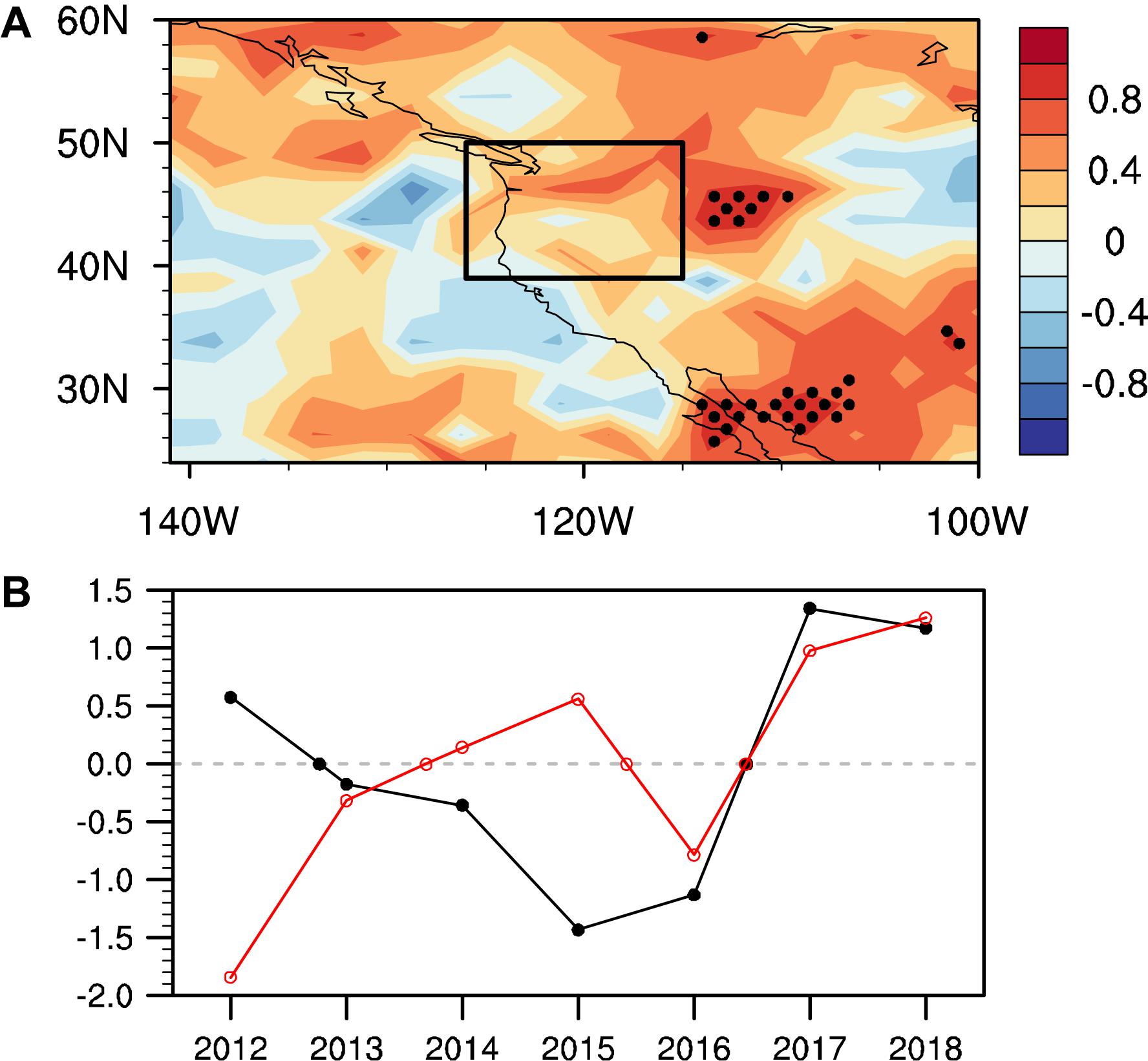
Figure 1. (A) Correlation coefficients between April precipitation predicted by the CFS using March data and April precipitation from the GPCP for 2012–2018. Dots indicate that correlations are significant at the 95% confidence level. The seasonal cycle and linear trend were removed from the original datasets before calculating correlation coefficients. (B) Standardized time series of April precipitation in the northwestern United States from the CFS using March data (red line) and April precipitation from the GPCP (black line) for 2012–2018. Data are averaged over 39°–50°N, 115°–126°W.

In addition, tropospheric weather and climate are closely linked to stratospheric processes (e.g., Hu and Guan, 2018; Hu et al., 2019; Zhao et al., 2019; He et al., 2020). Stratospheric signals generated by ozone depletion may propagate down to the troposphere and influence the tropospheric weather significantly (Bai et al., 2015; Hu et al., 2015; Manatsa and Mukwada, 2019; Wang et al., 2019; Zhang et al., 2019), including the tropospheric jet streams (Huang et al., 2017), surface temperature (Zhang et al., 2016, 2018; Huang et al., 2017; Hu et al., 2018; Huang and Tian, 2019), and precipitation (e.g., Luo et al., 2013; Ma et al., 2019). In particular, Ma et al. (2019) revealed that April P_NWUS can be modulated by March Arctic stratospheric ozone (ASO). They found that circulation anomalies associated with March ASO variations can propagate to the northwestern United States, leading to local circulation and water-vapor flux anomalies that can affect April P_NWUS. This motivates us to investigate whether the March ASO, which has a leading influence on the surface climate in the Northern Hemisphere (Smith and Polvani, 2014; Calvo et al., 2015; Xie et al., 2016, 2017a,b, 2018; Ivy et al., 2017; Ma et al., 2019), can be used along with other factors as a predictor of April P_NWUS in a statistical model. Results from this new statistical model will be compared with those of the CFS to assess improvements in the predictability of April P_NWUS.

In this paper, we develop a linear regression model using the observed March ASO and regional circulation signals to predict the April P_NWUS. The remainder of the paper is organized as follows. The data, simulations, and methods used in this study are described in section “Data.” The predictors and underlying mechanism are presented in section “Selecting Factors for April P_NWUS Predictions.” Section “Development of a Linear Regression Model to Predict April P_NWUS” describes the linear regression model used for April P_NWUS predictions and validates the model using observations and simulations. Results and conclusions are presented in section “Conclusion.”

Data

Data

The monthly mean partial ozone column averaged for the latitude of 60°–90°N at an altitude of 100–50 hPa after removing the linear trend and seasonal cycle is defined as the ASO index in this paper. The ozone values used in this study are from the Stratospheric Water and OzOne Satellite Homogenized database (SWOOSH, Davis et al., 2016) for 1985–2018. The monthly mean zonal-mean dataset is at 2.5° × 2.5° spatial resolution and has 31 vertical levels (316–1 hPa). Xie et al. (2018) showed that the ASO from SWOOSH is in good agreement with that from the Global Ozone Chemistry and Related trace gas Data Records for the Stratosphere (GOZCARDS, 1985–2013) project (Froidevaux et al., 2015), with horizontal resolution of 10° × 10°, extending from the surface to 0.1 hPa (25 levels).

Monthly precipitation employed in this study is taken from two sources: the GPCP monthly precipitation dataset provided by the NOAA/OAR/ESRL PSD, Boulder, CO, United States with a horizontal resolution of 2.5° × 2.5° (Adler et al., 2003) and the Global Precipitation Climatology Centre (GPCC) with a horizontal resolution of 1.0° × 1.0° (Schneider et al., 2008). Geopotential height and winds are obtained from the National Centers for Environmental Prediction-Department of Energy (NCEP-DOE) dataset.

Following Ma et al. (2019) who found that March ASO can significantly influence the April P_NWUS, the P_NWUS is defined as the area of 39°–50°N and 115°–126°W in this paper. To understand the characteristics of precipitation in the studied area, Figures 2A,B show the climatology of April P_NWUS. It is evident that the spring P_NWUS is increasing from the southeast to the northwest and that the primary mode of precipitation variability in this area shows a unified change (Figures 2C,D), indicating that the P_NWUS changes can be investigated as a whole. In addition, the April P_NWUS exhibits evident interannual changes, and the two sets of precipitation data show a high degree of consistency (Figure 2E).

FIGURE 2

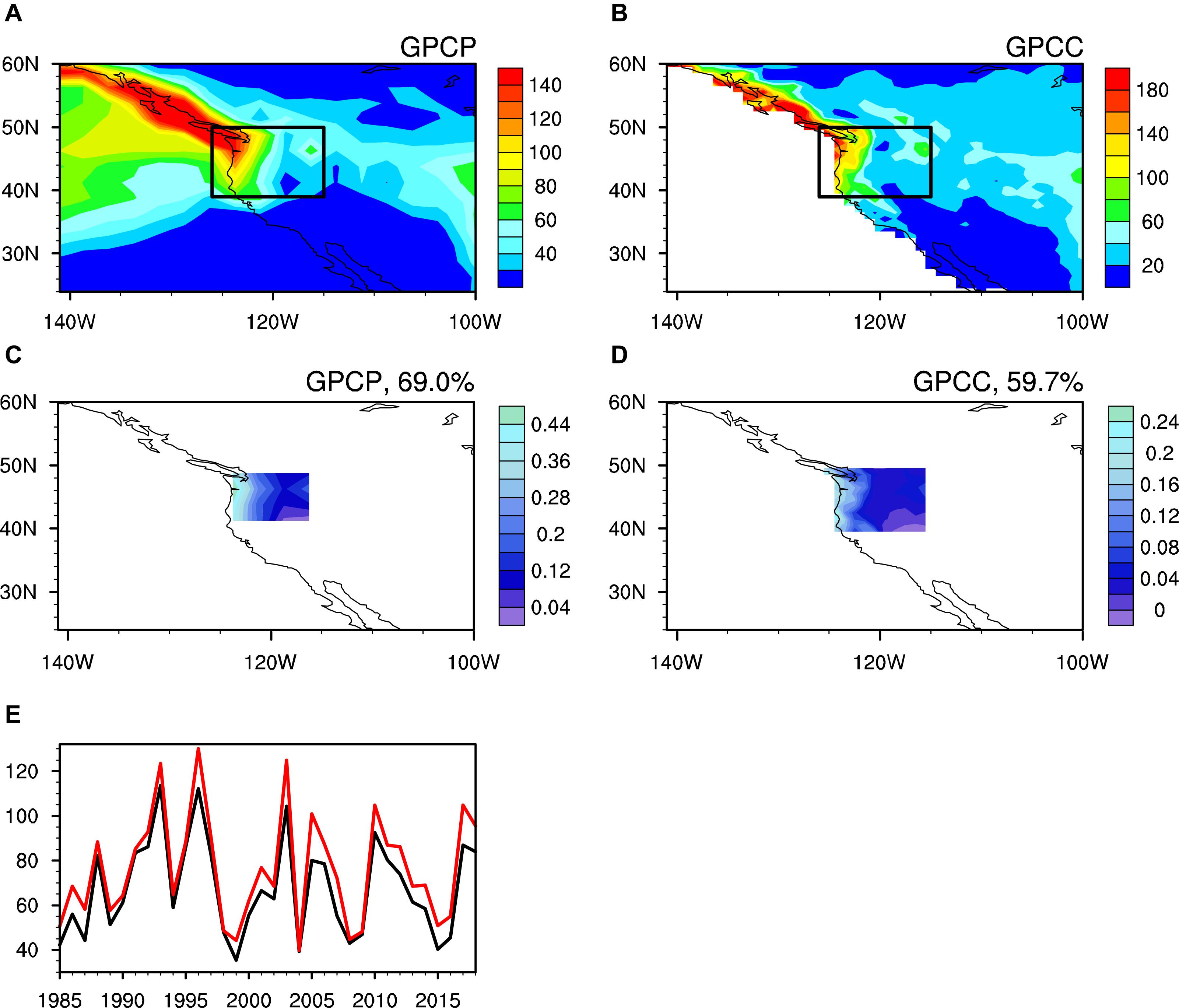
Figure 2. (A,B) Climatological values for April precipitation (mm/month) in the northwestern United States for 1985–2018 from the (A) GPCP and (B) GPCC. Black rectangles denote the study area (northwestern United States). (C,D) First leading EOF of April precipitation anomalies in the study area for the period 1985–2018 from the (C) GPCP and (D) GPCC. (E) Time series of April precipitation (mm/month) over the northwestern United States (P_NWUS) averaged over the region 39°–50°N, 115°–126°W from the GPCP (black line) and GPCC (red line).

The output from the CFS developed by the NCEP is also used in this paper. The CFS is a fully coupled operational dynamical seasonal prediction system (Saha et al., 2006). Its atmospheric component is the NCEP Global Forecast System model used for operational weather forecasting (Moorthi et al., 2001) except at a coarser horizontal resolution. Its oceanic component is the NOAA Geophysical Fluid Dynamics Laboratory Modular Ocean Model V3.0 (Pacanowski and Griffies, 1998). It adopts a spectral triangular truncation of 62 waves (T62) in the horizontal and 64 sigma layers in the vertical. The zonal resolution of the model is 1.0°, and its meridional resolution is 1/3° between 10°S and 10°N, increasing gradually with latitude before becoming 1° poleward of 30°S and 30°N. We used the monthly data of CFS from 1985 to 2018, including the reforecast (1985–2010) and the forecast period (2011–2018), both of which are a 9-month integration, and we adopted the data starting integration from 00 UTC.

Simulations

The National Center for Atmospheric Research’s Community Earth System Model (CESM) version 1.0.6 has been applied in this study to demonstrate the relationship between April P_NWUS and the predictors. CESM is a fully coupled global climate model that incorporates interactive atmospheric (CAM/WACCM), ocean (POP2), land (CLM4), and sea ice (CICE) components. The atmospheric component used in this study is the Whole Atmosphere Community Climate Model (WACCM), version 4 (Marsh et al., 2013). WACCM4, as a climate model, has a detailed middle-atmosphere chemistry and a finite-volume dynamical core, extending from the surface to ∼140 km with 66 vertical levels. The interactive chemistry employed in this paper is disabled. The horizontal resolution of the model is 1.9° × 2.5° (latitude × longitude) for the atmosphere and approximately the same for the ocean.

We conducted a transient experiment (1955–2005) using CESM incorporating both natural and anthropogenic external forcings, including spectrally resolved solar variability (Lean et al., 2005), transient greenhouse gases (GHGs) (from scenario A1B of IPCC 2001), volcanic aerosols (from the Stratospheric Processes and their Role in Climate (SPARC) Chemistry–Climate Model Validation (CCMVal) REF-B2 scenario recommendations), a nudged quasi-biennial oscillation (QBO) (the time-series in CESM is based on the observed climatology over the period 1955–2005), and ozone taken from the CMIP5 ensemble mean ozone output. All of the forcing data used in this study can be obtained from the CESM model input data repository.

Methods

Holdout Method

The holdout method, sometimes called test sample estimation, relies on a single partitioning of the data. For example, the whole time series is divided into two parts: the period from 1985 to 2007 is the training period, and the period from 2008 to 2018 is the hindcasting period.

Running Holdout Method

This method only differs from the holdout method in its use of a variable-length training period that changes with the hindcasting time point. That is, the required set of regression coefficients and constants are based on the time series before each hindcasting target point. The base period is the shortest training period.

Anomaly Sign Consistency

The anomaly sign consistency (P) is used to compare the observed and fitted April P_NWUS (Ruan et al., 2015), as shown in the following equation:

$$P=\frac{N^{\text{c}}}{N},(1)$$

where N^c represents the number of cases when the observed and fitted P_NWUS are both in positive or negative anomalies at the same time, and N represents the sample size.

Root-Mean-Squared Errors

The root-mean-squared errors (RMSEs) proposed in this paper are calculated based on a leave−1−year-out method. During 1985–2018 (34 years), 34 consecutive empirical models are produced after each one data point is left out. The remaining 33 data points are used to establish the linear regression model to forecast the 1 year that is left out. The RMSEs are calculated based on the observed and the predicted precipitation. More details can be found in Xie et al. (2019).

Selecting Factors for April P_NWUS Predictions

Figure 3A presents correlation coefficients between the March ASO index and April precipitation anomalies in the western United States. A strong negative relationship between March ASO and April precipitation variations is found in the northwestern United States. The time series of the March ASO index and April P_NWUS are shown in Figure 3C, indicating a significant correlation (95% confidence level) with a correlation coefficient of −0.44 between the two time series. It suggests that March ASO is linked to April P_NWUS variations with a lead time of 1 month. This delayed effect can be explained by the process involved in ASO circulation effects; i.e., stratospheric circulation anomalies caused by ASO need a month to propagate to the troposphere in the Northern Hemisphere middle latitudes (Smith and Polvani, 2014; Calvo et al., 2015; Xie et al., 2016; Ivy et al., 2017). Results from the GPCC (Figures 3B,D) agree with those from the GPCP (Figures 3A,C).

FIGURE 3

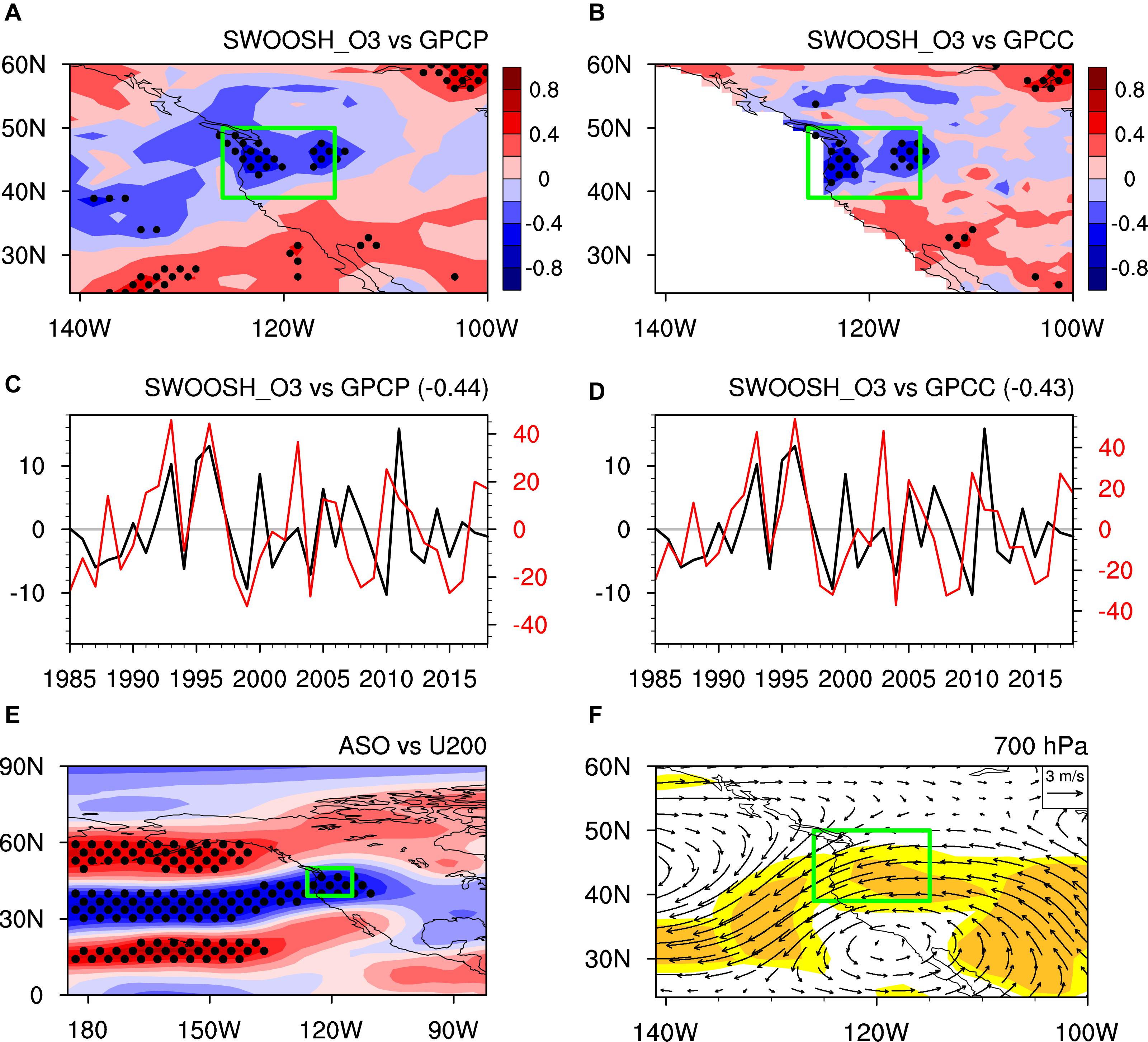
Figure 3. (A) Correlation coefficients between the March ASO index from SWOOSH and April precipitation anomalies from the GPCP during 1985–2018. Dots indicate areas that are statistically significant at the 95% confidence level. The linear trend was removed from the original datasets before calculating correlation coefficients. (C) Time series of March ASO (× –1) from SWOOSH (DU; black line) and April P_NWUS (mm/month; red line) anomalies from the GPCP after removing the linear trend for 1985–2018. The correlation coefficient between the two time series is shown in the upper right corner. (B,D) As in panels (A,C), but for precipitation from the GPCC. (E) Correlation coefficients between the March ASO index from SWOOSH and April zonal wind anomalies (m/s) from NCEP2 at 200 hPa for 1985–2018. Dots indicate areas that are statistically significant at the 95% confidence level. (F) Differences in composite April wind from NCEP2 (vectors; m/s) between positive and negative March ASO anomaly events at 700 hPa for 1985–2018 significant at the 90% (light yellow shading) and 95% (dark yellow shading) confidence levels, respectively. See Table 1 for specific March ASO anomaly events. The green rectangle indicates the study area (northwestern United States).

TABLE 1

Table 1. Selected positive and negative March ASO and April H700_WNA anomaly events during 1985–2018 identified according to their standard deviations.

As the physical mechanisms linking March ASO and April P_NWUS have been explored by Ma et al. (2019) in detail using observations and model verification based on time-slice and transient experiments, here we only briefly describe the physical connection between March ASO and April P_NWUS. The correlation coefficients between March ASO and April zonal wind at 200 hPa are shown in Figure 3E. The intensity of April zonal wind over the North Pacific is noticeably affected by variations in March ASO, showing a triple mode with a zonal distribution. This means that when March ASO increases, zonal wind in the higher and lower latitudes of the North Pacific displays a positive anomaly, whereas zonal wind in the mid-latitude North Pacific demonstrates a negative anomaly (Figure 3E). These circulation anomalies can extend eastward to the western United States, influencing regional circulation and climate (Xie et al., 2018; Ma et al., 2019). Specific wind anomalies related to March ASO variations in the troposphere are shown in Figure 3F. Wind anomalies in the northwestern United States are dominated by the northeast wind when the March ASO is abnormally high. These conditions suppress local precipitation. Opposite results are found when March ASO is abnormally low. Given this relationship between March ASO and April P_NWUS, we select March ASO as the first factor in our model for predicting P_NWUS.

The correlation coefficients in Figure 3 suggest that the ASO only partially explains variations in P_NWUS. Therefore, other factors that affect P_NWUS must be identified. First, we divide the variations of P_NWUS into two parts: the ASO-related part (P_{NWUS_ASO}) and the remainder (P_{NWUS_NOASO}). The P_{NWUS_ASO} is obtained by regressing P_NWUS variations onto ASO, and P_{NWUS_NOASO} = P_NWUS – P_{NWUS_ASO}. P_{NWUS_NOASO} describes P_NWUS variations with the effects of ASO removed.

To simplify the problem, we investigate the circulation factors that directly affect precipitation. To find a factor for P_{NWUS_NOASO}, correlation coefficients between April P_{NWUS_NOASO} variations and simultaneous geopotential height anomalies (after removing the signals of March ASO from the geopotential height) at 200, 500, and 700 hPa are shown in Figure 4. There are 17 regions with significant correlation identified in Figure 4. The circulation anomalies in these regions may be factors involved in the remaining precipitation (P_{NWUS_NOASO}) variations. RMSEs are calculated for each potential factor to find the best factor in the model. The three factors with the smallest RMSE are shown in the row labeled “Step 1” in Table 2. The factor H700_WNA (geopotential height in western North America at 700 hPa) has the lowest RMSE (14.09 mm), and the correlation coefficient between this factor and P_{NWUS_NOASO} is the largest and is significant at the 95% confidence level. This factor also passes the T and F tests. Therefore, April H700_WNA is provisionally selected as the second factor in the model for predicting P_NWUS.

TABLE 2

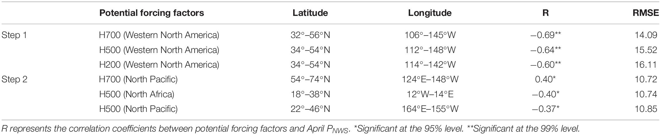
Table 2. The three potential forcing factors with the lowest root-mean-squared errors (RMSEs) in each step.

FIGURE 4

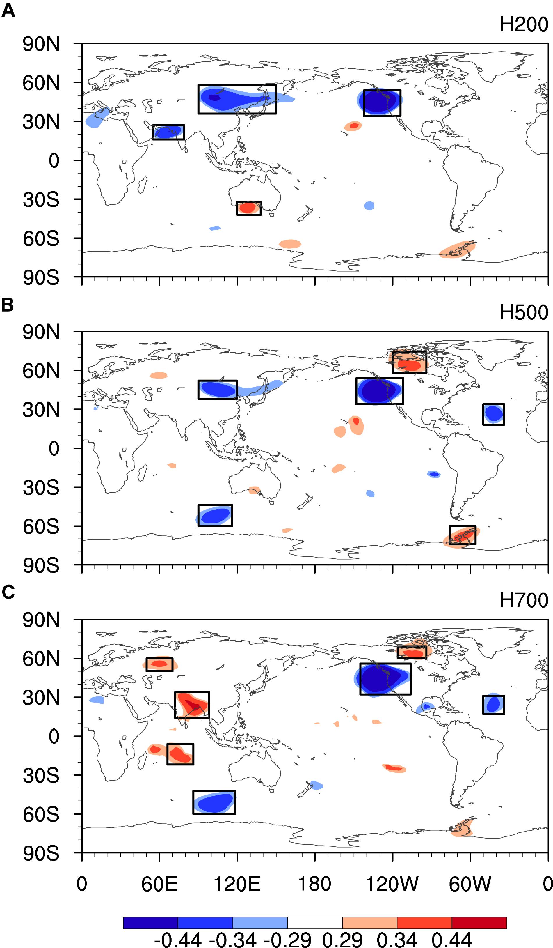
Figure 4. Correlation coefficients between April P_{NWUS_NOASO} and simultaneous geopotential height at (A) 200, (B) 500, and (C) 700 hPa during 1985–2018. The ASO signals were removed from the geopotential height before calculating the correlation coefficient. Boxes are the regions of the potential factors. Shaded areas indicate statistically significant correlation at (at least) the 90, 95, and 99% confidence levels.

Next, we discuss the physical processes involved in the effects of April H700_WNA on simultaneous P_{NWUS_NOASO}. Figure 5A shows climatological values for April wind, which indicate that the northwestern United States is dominated by the west wind. Figure 5B presents differences in composite April wind between positive and negative April H700_WNA anomaly events at 700 hPa. Circulation anomalies related to April H700_WNA are anti-cyclonic in western North America when April H700_WNA is abnormally high. This corresponds to a divergence of the airflow, which is unfavorable for water-vapor transport from the North Pacific to this area and strengthens dry, cold air transport from the north. Because anti-cyclonic circulation tends to suppress convective activity, a pressure–longitude cross-section of the differences in composite April vertical-longitude wind between positive and negative H700_WNA anomaly events is shown in Figure 5C. The northwestern United States is covered by an anomalous downwelling airflow during positive H700_WNA events, suppressing convective activity. This less water-vapor and downwelling airflow anomaly results in a decrease in April P_NWUS during positive H700_WNA anomaly events, with the opposite occurring during negative H700_WNA anomaly events.

FIGURE 5

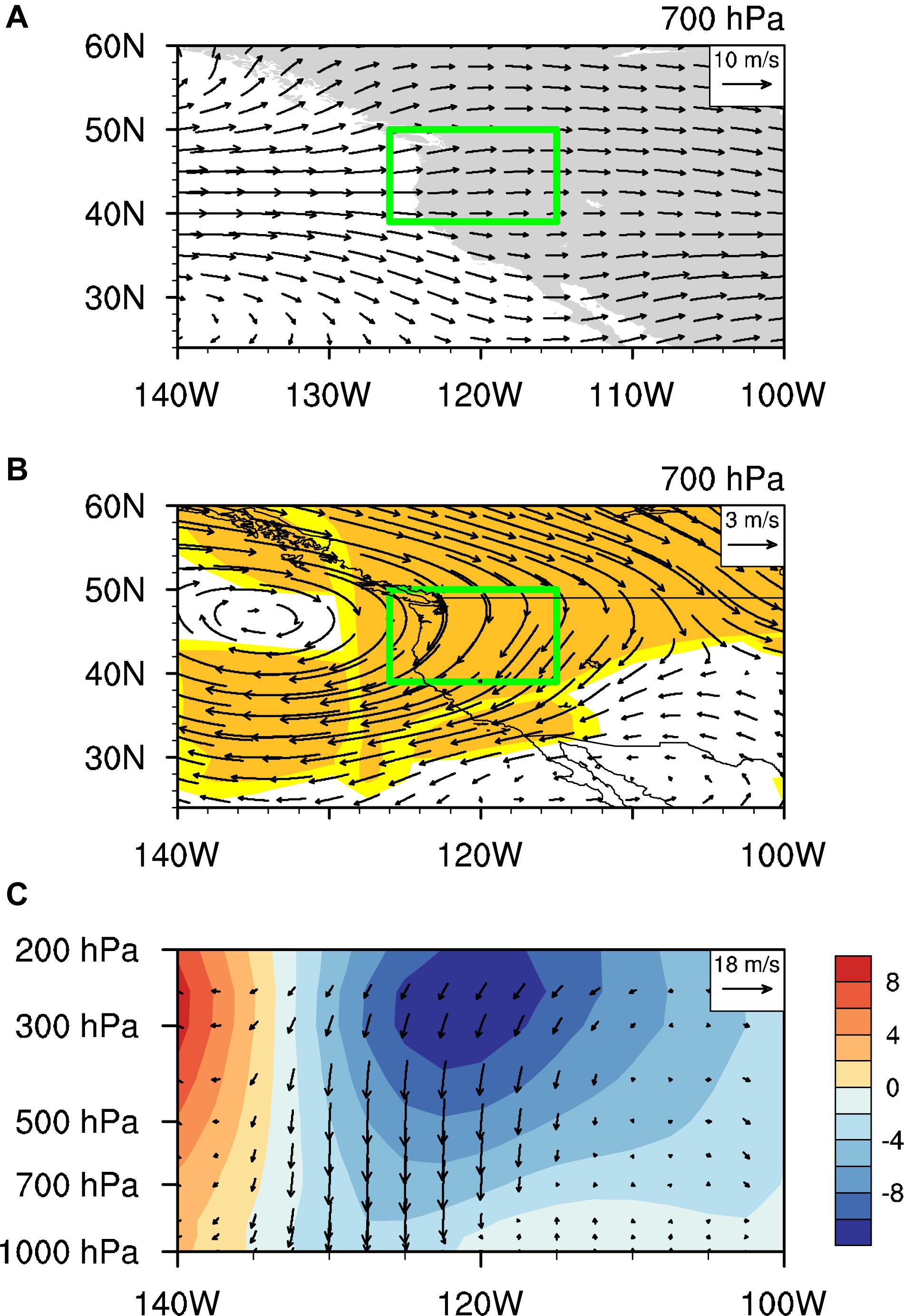
Figure 5. (A) Climatological values of April wind from NCEP2 (vectors; m/s) at 700 hPa for 1985–2018. Green rectangles indicate the study area. (B) Differences in composite April wind from NCEP2 (vectors; m/s) between positive and negative April H700_WNA anomaly events at 700 hPa during 1985–2018 significant at the 90% (light yellow shading) and 95% (dark yellow shading) confidence levels. (C) Differences in composite April wind (vectors; m/s) between positive and negative April H700_WNA anomaly events for 1985–2018. Colored regions represent the differences in the composite meridional wind. Vectors represent the composite zonal and vertical winds, where the vertical velocity has been converted to the magnitude of zonal wind. See Table 1 for specific April H700_WNA anomaly events.

The above analysis demonstrates that circulation anomalies (H700_WNA anomalies) can modulate simultaneous P_{NWUS_NOASO} and supports our selection of H700_WNA as a factor in the statistical model. Other factors contributing to P_{NWUS_NOASO} are investigated next. First, we divide the variations of P_{NWUS_NOASO} into two parts: the H700_WNA-related part (P_{NWUS_NOASO_H700}) and the remainder (P_{NWUS_NOASO_NOH700}). P_{NWUS_NOASO_H700} is obtained by regressing P_{NWUS_NOASO} variations onto H700_WNA, and P_{NWUS_NOASO_NOH700} = P_{NWUS_NOASO} – P_{NWUS_NOASO_H700}. P_{NWUS_NOASO_NOH700} describes P_NWUS variations with the effects of ASO and H700_WNA removed.

Figure 6 shows the correlation coefficients between April P_{NWUS_NOASO_NOH700} and simultaneous geopotential height anomalies (after removing the signals of March ASO and April H700_WNA from the geopotential height). Thirty-two potential factors are identified. The three factors with the smallest RMSE are shown in the row labeled “Step 2” in Table 2. The factor with the lowest RMSE is the geopotential field located in the North Pacific at 700 hPa. Although the correlation coefficient between this factor and P_{NWUS_NOASO_NOH700} is significant at the 95% confidence level, it passes neither the t-test nor the F-test. This suggests that, in terms of the circulation field, there are no remaining factors that can explain variations of P_{NWUS_NOASO_NOH700} better. Thus, only ASO and H700_WNA are selected as predictors in the model, and no additional factors are investigated.

FIGURE 6

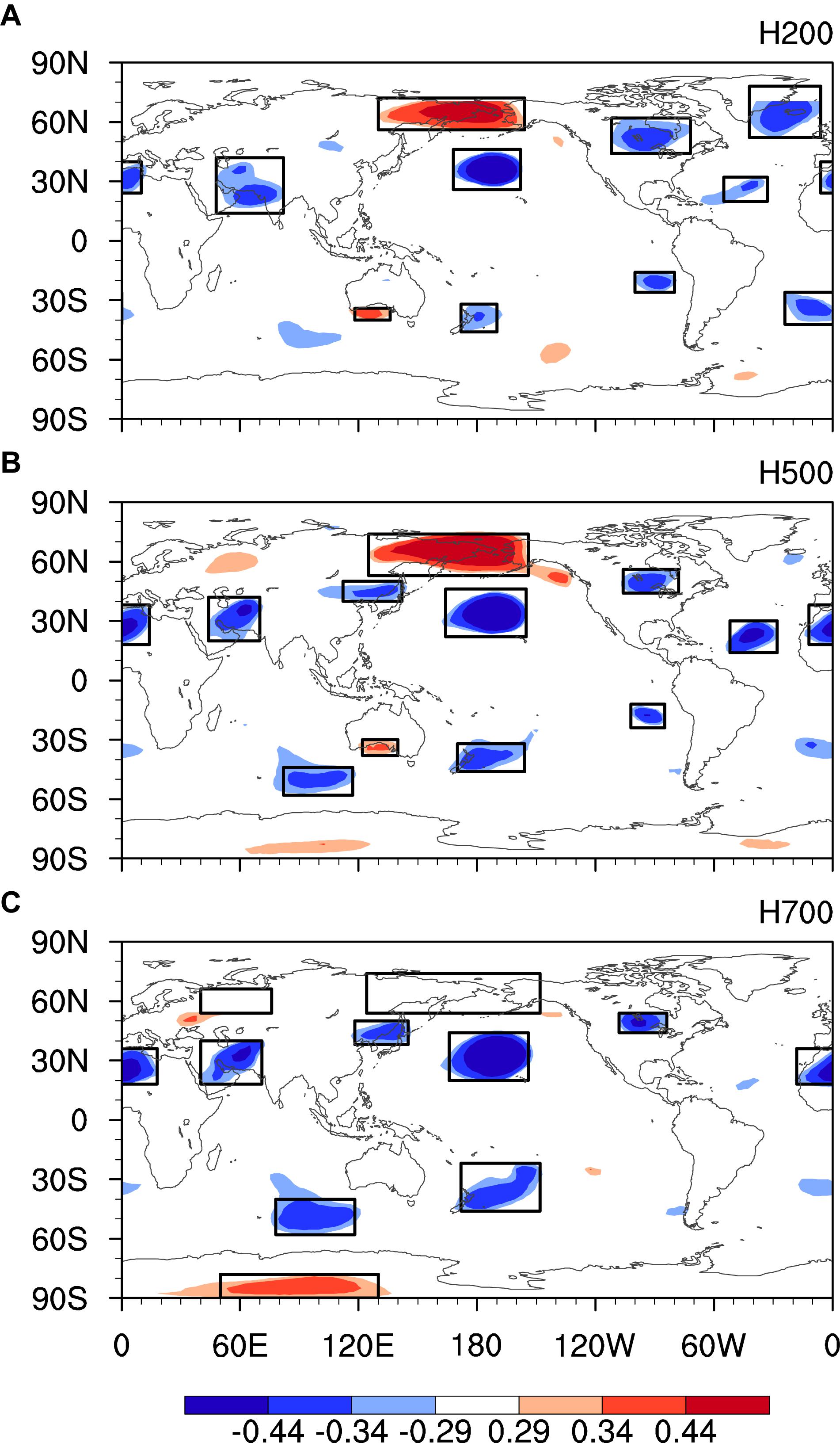
Figure 6. Correlation coefficients between April P_{NWUS_NOASO_NOH700} and simultaneous geopotential height at (A) 200, (B) 500, and (C) 700 hPa during 1985–2018. The ASO and H700_WNA signals were removed from the geopotential height before calculating the correlation coefficient. Boxes are the regions of the potential factors. Shaded areas indicate statistically significant correlation at (at least) the 90, 95, and 99% confidence levels.

Development of a Linear Regression Model to Predict April P_NWUS

Local precipitation may be affected by both linear and non-linear climate forcing factors. However, Zorita and Von Storch (1999) pointed out that linear models offer a clearer physical interpretation. Guo et al. (2012) indicated that linear models perform well on monthly mean seasonal time scales. Thus, we construct a linear regression model to predict April P_NWUS. Two factors, March ASO and April H700_WNA, are selected for use in the model.

The ASO leads P_NWUS variations by about 1 month and can thus be considered as a predictor. However, the H700_WNA and P_NWUS correlation is simultaneous (April), so April H700_WNA cannot be used in a statistical model for predicting April P_NWUS. The CFS developed by NCEP is suitable for evaluating circulation variations in the northwestern United States; i.e., April H700_WNA predicted by the CFS using March data is significantly correlated (95% confidence level) with April H700_WNA from NCEP2 with a correlation coefficient of 0.33 (Figure 7A). Thus, we use observed March ASO and April H700_WNA predicted by the CFS using March data as the two predictors in the linear regression model. Note from the standardized time series of the two predictors (Figure 7B) that they undergo significant interannual variations and are independent of each other (r = 0.02, not significant at the 95% confidence level).

FIGURE 7

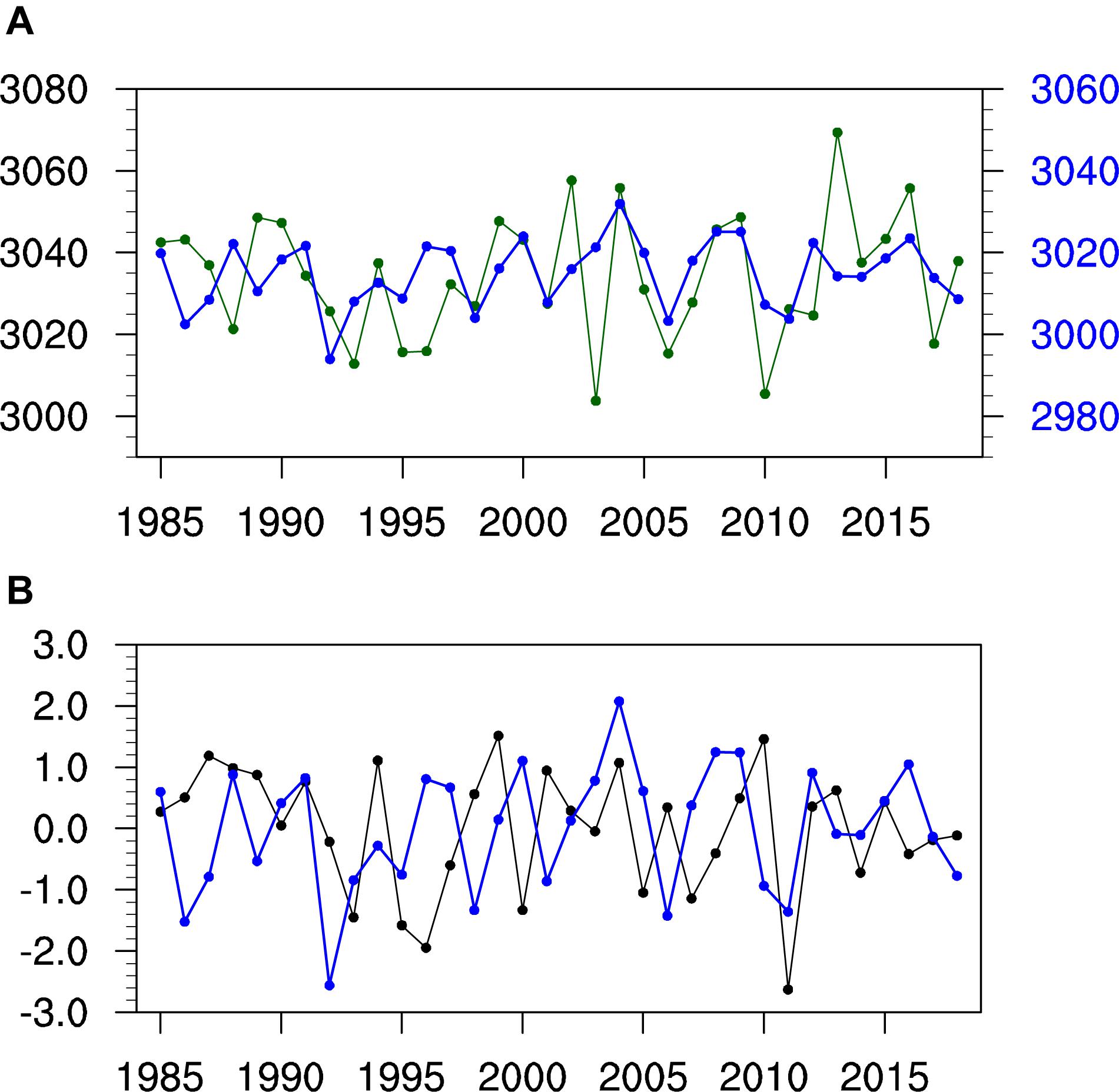
Figure 7. (A) Observed (green line) and predicted (blue line) April H700_WNA variations for 1985–2018. The observed April H700_WNA is from NCEP2, and the predicted April H700_WNA is from the CFS using March data. (B) Standardized time-series of March ASO (black line) and April H700_WNA predicted by the CFS using March data (blue line) for 1985–2018.

According to the holdout method, we use these two predictors and P_NWUS to establish a linear regression model for the training period (1985–2007) as follows:

$${\text{P}}_{NWUS}=3086.26-1.09\times \text{ASO}-1.00\times {\mathrm{H700}}_{WNA},(2)$$

where the units of April P_NWUS, March ASO, and April H700_WNA are mm, DU, and m, respectively.

The time series of observed, fitted, and predicted P_NWUS according to the above linear regression model are shown in Figure 8A. During the training period (1985–2007), the correlation coefficient and anomaly sign consistency rate between the observed and fitted P_NWUS are 0.44 (significant at the 95% confidence level) and 48%, respectively. During the test period (2008–2018), these values between the observed and predicted P_NWUS are 0.50 (significant at the 90% confidence level) and 46%, which are similar to the values during the training period. To further examine the stability and predictability of the linear regression model, we re-predict April P_NWUS during the test period (2008–2018) using the running holdout model (see section “Data”) – i.e., we train the linear regression model on a different period. The results are shown in Figure 8B. During the test period (2008–2018), the correlation coefficient and anomaly sign consistency rate between the observed and predicted P_NWUS are 0.53 (significant at the 90% confidence level) and 46%, respectively. This is consistent with the results shown in Figure 8A, indicating that the linear regression model is stable and reliable.

FIGURE 8

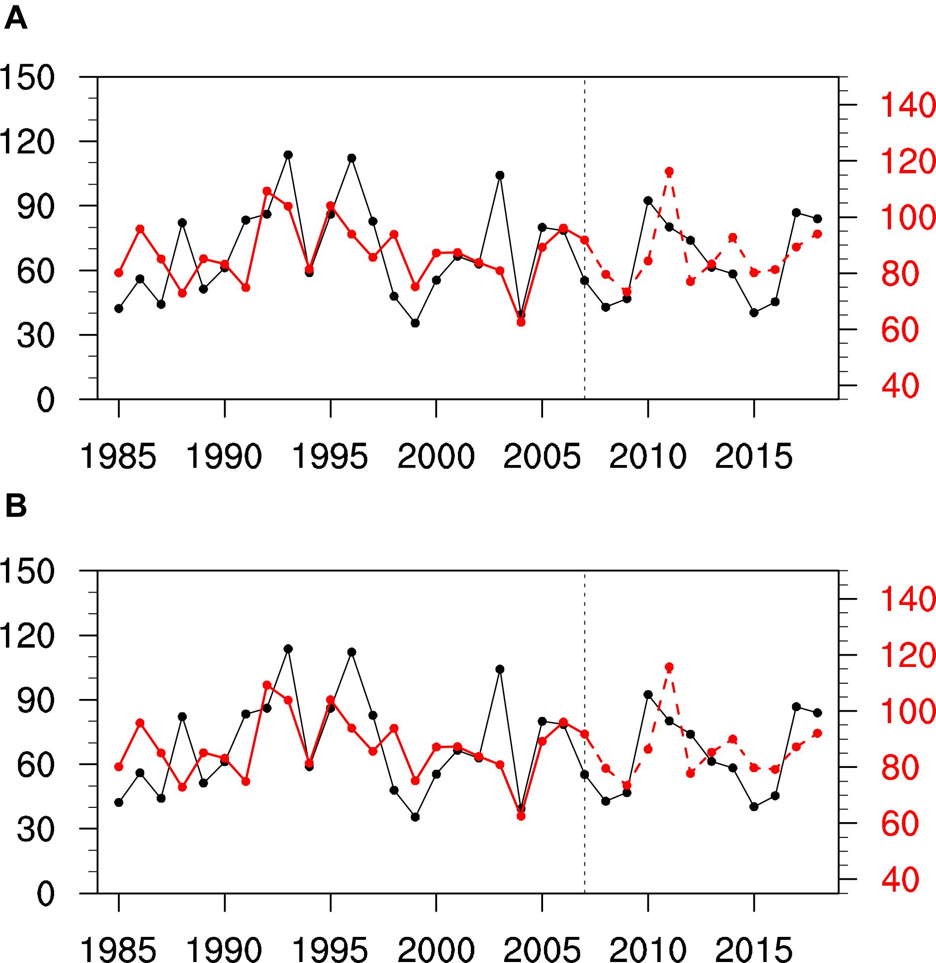
Figure 8. (A) Observed April P_NWUS (black line) and fitted (solid red line) and predicted (dashed red line) April P_NWUS variations from the linear regression model using observed March ASO and April H700_WNA predicted by the CFS using March data for 1985–2018. The training period is 1985–2007, and the independent test period is 2008–2018. (B) As in panel (A), except that the predicted April P_NWUS during 2008–2018 is based on the running holdout model.

To further test the robustness of the linear regression model with a longer time series, a transient experiment is implemented next. Details of the model and experiment are provided in section “Data.” The results are shown in Figure 9. Significant correlations are found between the CESM-simulated and fitted April P_NWUS during the training period with a correlation coefficient of 0.63 (significant at the 99% confidence level) and between the CESM-simulated and predicted April P_NWUS with a correlation coefficient of 0.75 (significant at the 99% confidence level) during the test period. The transient experiment illustrates that a strong connection exists among March ASO, April H700_WNA, and April P_NWUS and that the linear regression model is stable and reliable, supporting the results from observations described above.

FIGURE 9

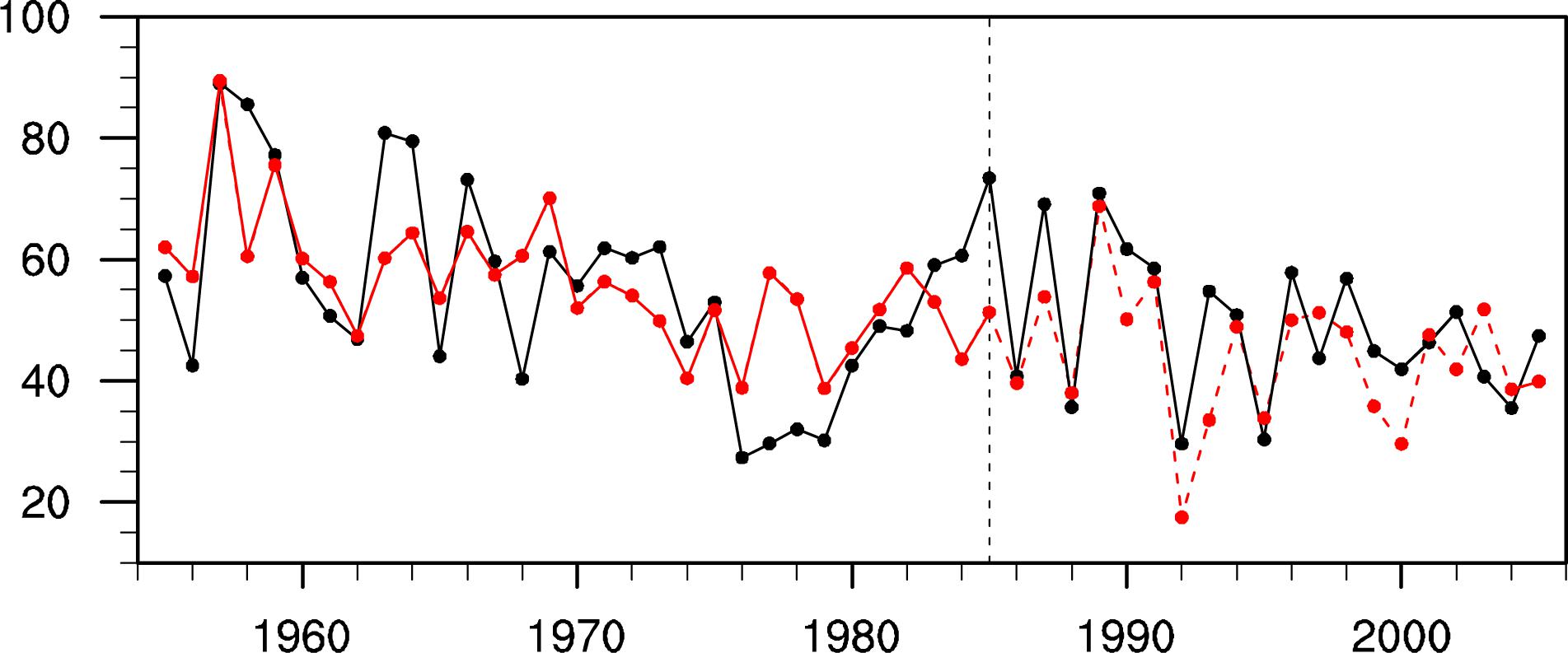
Figure 9. Simulated (black line), fitted (solid red line) and predicted (dashed red line) April P_NWUS variations. The fitted and predicted P_NWUS is calculated based on the linear regression model using CESM-specified March ASO and CESM-simulated H700_WNA. The training period is 1955–1985, and the test period is 1986–2005.

Note that the magnitude of the fitted and predicted precipitation variations is larger than that in the observations (Figure 8). This may be because the April H700_WNA predicted by the CFS using March data is smaller than that observed (Figure 7A). To address this issue, we correct the April H700_WNA predicted by the CFS using March data by adding a constant value of 19.26 (Figure 10A, the difference between the average of observed April H700_WNA and April H700_WNA predicted by the CFS in March for the period 1985–2018). Then, we use March ASO and the corrected April H700_WNA to build the linear regression model for predicting April P_NWUS. The new model is shown as follows:

FIGURE 10

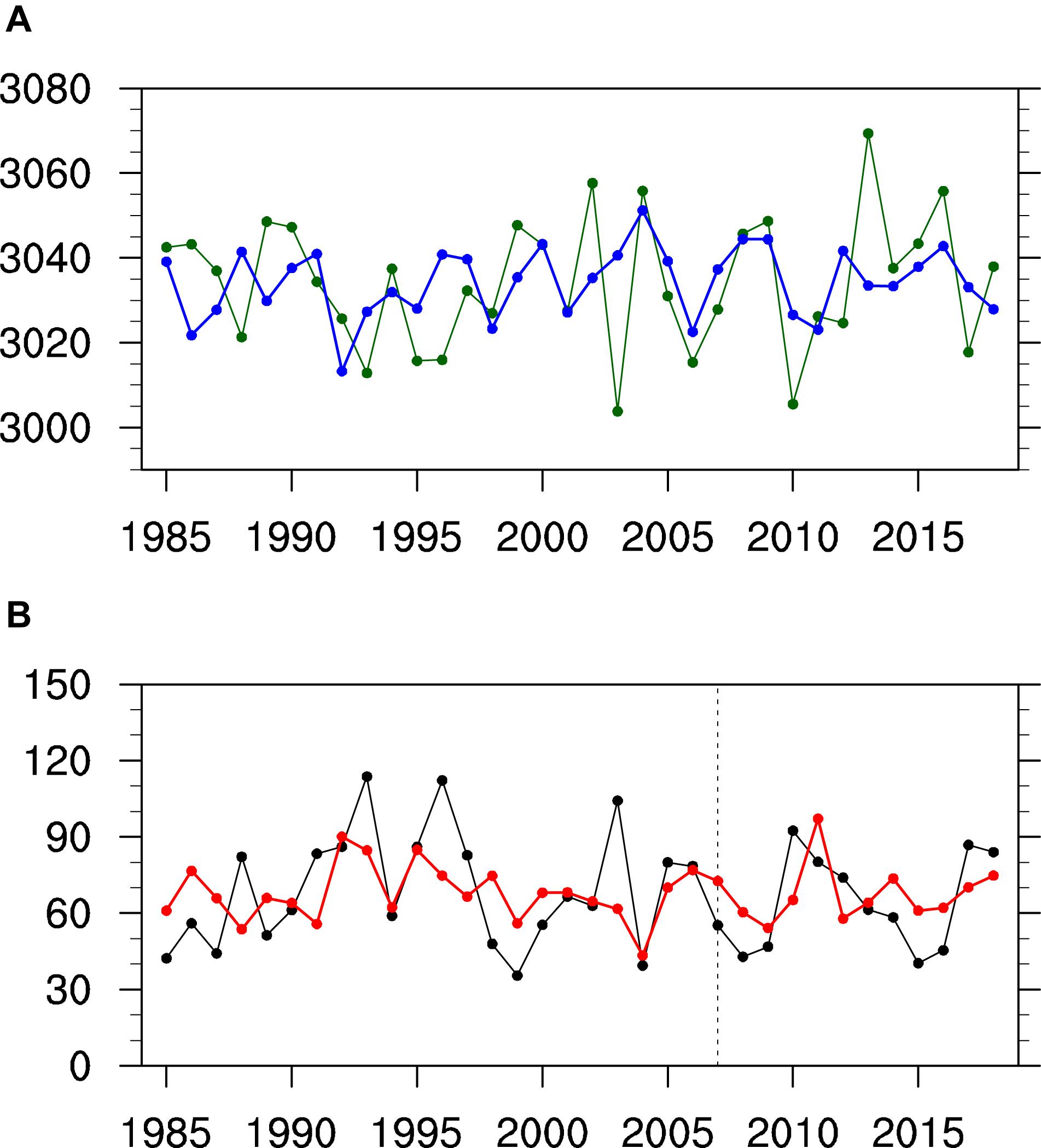
Figure 10. (A) Is the same as Figure 7A and (B) is the same as Figure 8A, except that the CFS-predicted April H700_WNA using March data has been corrected by adding a constant value of 19.26.

$${\text{P}}_{NWUS}=3105.52-1.09\times \text{ASO}-1.00\times {\mathrm{H700}}_{WNA}(3)$$

The results shown in Figure 10B are similar to those shown in Figure 8A. Note that the magnitude of the fitted and predicted precipitation variations is closer to that of observations. This suggests that the agreement of the predicted P_NWUS with observations was improved.

In addition, the correlation coefficients among observed P_NWUS, ASO, H700_WNA, and fitted P_NWUS variations are also significant at the 95% confidence level based on the Monte Carlo test (not shown), which supports the conclusions based on the Student’s t-test.

Conclusion

The March ASO can be used as a predictor for April P_NWUS because its anomalies significantly influence April tropospheric winds over the North Pacific with a triple mode. Circulation anomalies can extend eastward to western North America, causing wind anomalies in the northwestern United States in the troposphere. For example, the northwestern United States is dominated by northeast wind anomalies when there is an increase in March ASO. These conditions weaken local precipitation. When the April H700_WNA is abnormally high, circulation anomalies are anti-cyclonic in the western United States, which is unfavorable for water-vapor transport from the North Pacific to this region. Furthermore, the northwestern United States is covered by an anomalous downwelling airflow suppressing convective activity. This leads to less P_NWUS.

Based on observed March ASO and April H700_WNA predicted by the CFS using March data, we developed a linear regression model to predict the April P_NWUS with a 1-month lead. Results show that the linear regression model not only reproduces the historical April P_NWUS during the training period, but its predictions are also robust and reliable for the independent test period. Results from WACCM4 also support conclusions drawn from the analysis of observations.

Finally, we compare the April P_NWUS directly predicted by the CFS using March data to that predicted by the statistical model in March described here. The correlation coefficient between the observed April P_NWUS and that predicted by the CFS using March data is 0.25 during 2012–2018 (before 2011, no CFS-predicted April P_NWUS data are available), whereas the correlation coefficient between the observed April P_NWUS and that predicted by the linear regression model is 0.53. This indicates that, at this stage, the linear regression model is better able to predict April P_NWUS than CFS at a lead time of 1 month. In summary, the linear regression model described here can be used to improve predictions of April P_NWUS variations.

Data Availability Statement

The datasets generated for this study are available on request to the corresponding author.

Author Contributions

XM and FX designed the study, contributed to the data analysis and interpretation, and manuscript writing.

Funding

This work was supported by the National Natural Science Foundation of China (91837311 and 41975047) and Natural Science Basic Research Plan in Shaanxi Province of China (2019JQ-278).

Conflict of Interest

The authors declare that the research was conducted in the absence of any commercial or financial relationships that could be construed as a potential conflict of interest.

Acknowledgments

We acknowledge the ozone datasets from the SWOOSH, precipitation data from the GPCC, GPCP, and CFS, and meteorological fields from NCEP2. We thank NCAR for providing the CESM model. This research was supported by Super Computing Center of Beijing Normal University, user name is xiefei.

References

Adler, R. F., Huffman, G. J., Chang, A., Ferraro, R., Xie, P. P., Janowiak, J., et al. (2003). The version-2 global precipitation climatology project (GPCP) monthly precipitation analysis (1979–present). J. Hydrometeorol. 4, 1147–1167. doi: 10.1175/1525-7541(2003)004<1147:tvgpcp>2.0.co;2

CrossRef Full Text | Google Scholar

Andreadis, K. M., Clark, E. A., Wood, A. W., Hamlet, A. F., and Lettenmaier, D. P. (2005). Twentieth-century drought in the conterminous United States. J. Hydrometeorol. 6, 985–1001. doi: 10.1175/jhm450.1

CrossRef Full Text | Google Scholar

Bai, K., Liu, C., Shi, R., and Gao, W. (2015). Comparison of Suomi-NPP OMPS total column ozone with Brewer and Dobson spectrophotometers measurements. Front. Earth Sci. 9:369. doi: 10.1007/s11707-014-0480-5

CrossRef Full Text | Google Scholar

Calvo, N., Polvani, L. M., and Solomon, S. (2015). On the surface impact of Arctic stratospheric ozone extremes. Environ. Res. Lett. 10:094003. doi: 10.1088/1748-9326/10/9/094003

CrossRef Full Text | Google Scholar

Chu, J. T., Xia, J., and Xu, C. Y. (2008). Statistical downscaling the daily precipitation for climate change scenarios in Haihe River basin of China. J. Nat. Res. 23, 1068–1077.

Google Scholar

Davis, S. M., Rosenlof, K. H., Hassler, B., Hurst, D. F., Read, W. G., Vomel, H., et al. (2016). The stratospheric water and ozone satellite homogenized (SWOOSH) database: a long-term database for climate studies. Earth Syst. Sci. Data 8, 461–490. doi: 10.5194/essd-8-461-2016

PubMed Abstract | CrossRef Full Text | Google Scholar

Fowler, H. J., Blenkinsop, S., and Tebaldi, C. (2007). Linking climate change modelling to impacts studies: recent advances in downscaling techniques for hydrological modelling. Int. J. Climatol. 27, 1547–1578. doi: 10.1002/joc.1556

CrossRef Full Text | Google Scholar

Froidevaux, L., Anderson, J., Wang, H. J., Fuller, R. A., Schwartz, M. J., Santee, M. L., et al. (2015). Global OZone Chemistry And Related trace gas Data records for the Stratosphere (GOZCARDS): methodology and sample results with a focus on HCl, H2O, and O-3. Atmos. Chem. Phys. 15, 10471–10507. doi: 10.5194/acp-15-10471-2015

CrossRef Full Text | Google Scholar

Goodess, C. M., and Palutikof, J. P. (1998). Development of daily rainfall scenarios for southeast Spain using a circulation-type approach to downscaling. Int. J. Climatol. 18, 1051–1083. doi: 10.1002/(sici)1097-0088(199808)18:10<1051::aid-joc304>3.0.co;2-1

CrossRef Full Text | Google Scholar

Guo, Y., Li, J., and Li, Y. (2012). A time-scale decomposition approach to statistically downscale summer rainfall over North China. J. Clim. 25, 572–591. doi: 10.1175/jcli-d-11-00014.1

CrossRef Full Text | Google Scholar

Harding, K. J., and Snyder, P. K. (2015). The relationship between the Pacific-North American teleconnection pattern, the Great Plains low-level jet, and North Central US heavy rainfall events. J. Clim. 28, 6729–6742. doi: 10.1175/jcli-d-14-00657.1

CrossRef Full Text | Google Scholar

Hatfield, J. L., and Dold, C. (2018). Agroclimatology and wheat production: coping with climate change. Front. Plant Sci. 9:224. doi: 10.3389/fpls.2018.00224

PubMed Abstract | CrossRef Full Text | Google Scholar

He, Y., Sheng, Z., and He, M. (2020). Spectral analysis of gravity waves from near space high-resolution balloon data in Northwest China. Atmosphere 11:133. doi: 10.3390/atmos11020133

CrossRef Full Text | Google Scholar

Hewitson, B. C., and Crane, R. G. (2006). Consensus between GCM climate change projections with empirical downscaling: precipitation downscaling over South Africa. Int. J. Climatol. 26, 1315–1337. doi: 10.1002/joc.1314

CrossRef Full Text | Google Scholar

Hu, D., and Guan, Z. (2018). Decadal relationship between the stratospheric Arctic vortex and Pacific decadal oscillation. J. Clim. 31, 3371–3386. doi: 10.1175/jcli-d-17-0266.1

CrossRef Full Text | Google Scholar

Hu, D., Guan, Z., Tian, W., and Ren, R. (2018). Recent strengthening of the stratospheric Arctic vortex response to warming in the central North Pacific. Nat. Commun. 9:1697. doi: 10.1038/s41467-018-04138-3

PubMed Abstract | CrossRef Full Text | Google Scholar

Hu, D., Guo, Y., and Guan, Z. (2019). Recent weakening in the stratospheric planetary wave intensity in early winter. Geophys. Res. Lett. 46, 3953–3962. doi: 10.1029/2019gl082113

CrossRef Full Text | Google Scholar

Hu, D., Tian, W., Xie, F., Wang, C., and Zhang, J. (2015). Impacts of stratospheric ozone depletion and recovery on wave propagation in the boreal winter stratosphere. J. Geophys. Res. Atmos. 120, 8299–8317. doi: 10.1002/2014jd022855

CrossRef Full Text | Google Scholar

Huang, J., and Tian, W. (2019). Eurasian Cold Air Outbreaks Under Different Arctic stratospheric polar vortex strengths. J. Atmos. Sci. 76, 1245–1264. doi: 10.1175/jas-d-18-0285.1

CrossRef Full Text | Google Scholar

Huang, J., Zhang, J. C., Zhang, Z. X., Xu, C. Y., Wang, B. L., and Yao, J. (2011). Estimation of future precipitation change in the Yangtze River basin by using statistical downscaling method. Stoch. Environ. Res. Risk Assess. 25, 781–792. doi: 10.1007/s00477-010-0441-9

CrossRef Full Text | Google Scholar

Huang, J. L., Tian, W. S., Zhang, J. K., Huang, Q., Tian, H. Y., and Luo, J. L. (2017). The connection between extreme stratospheric polar vortex events and tropospheric blockings. Q. J. R. Meteorol. Soc. 143, 1148–1164. doi: 10.1002/qj.3001

CrossRef Full Text | Google Scholar

Hughes, J. P., and Guttorp, P. (1994). A class of stochastic-models for relating synoptic atmospheric patterns to regional hydrologic phenomena. Water Resour. Res. 30, 1535–1546. doi: 10.1029/93wr02983

CrossRef Full Text | Google Scholar

Ivy, D. J., Solomon, S., Calvo, N., and Thompson, D. W. J. (2017). Observed connections of Arctic stratospheric ozone extremes to Northern Hemisphere surface climate. Environ. Res. Lett. 12:024004. doi: 10.1088/1748-9326/aa57a4

CrossRef Full Text | Google Scholar

Lean, J., Rottman, G., Harder, J., and Kopp, G. (2005). SORCE contributions to new understanding of global change and solar variability. Sol. Phys. 230, 27–53. doi: 10.1007/0-387-37625-9_3

CrossRef Full Text | Google Scholar

Lee, S. K., Mapes, B. E., Wang, C. Z., Enfield, D. B., and Weaver, S. J. (2014). Springtime ENSO phase evolution and its relation to rainfall in the continental U.S. Geophys. Res. Lett. 41, 1673–1680. doi: 10.1002/2013gl059137

CrossRef Full Text | Google Scholar

Li, L. F., Schmitt, R. W., and Ummenhofer, C. C. (2018). The role of the subtropical North Atlantic water cycle in recent US extreme precipitation events. Clim. Dyn. 50, 1291–1305. doi: 10.1007/s00382-017-3685-y

CrossRef Full Text | Google Scholar

Li, L. F., Schmitt, R. W., Ummenhofer, C. C., and Karnauskas, K. B. (2016). Implications of North Atlantic sea surface salinity for summer precipitation over the US midwest: mechanisms and predictive value. J. Clim. 29, 3143–3159. doi: 10.1175/jcli-d-15-0520.1

CrossRef Full Text | Google Scholar

Li, Y., and Smith, I. (2009). A statistical downscaling model for Southern Australia winter rainfall. J. Clim. 22, 1142–1158. doi: 10.1175/2008jcli2160.1

CrossRef Full Text | Google Scholar

Luo, J., Tian, W., Pu, Z., Zhang, P., Shang, L., Zhang, M., et al. (2013). Characteristics of stratosphere troposphere exchange during the Meiyu season. J. Geophys. Res. Atmos. 118, 2058–2072. doi: 10.1029/2012jd018124

CrossRef Full Text | Google Scholar

Ma, X., Xie, F., Li, J., Zheng, X., Tian, W., Ding, R., et al. (2019). Effects of Arctic stratospheric ozone changes on spring precipitation in the Northwestern United States. Atmos. Chem. Phys. 19, 861–875.

Google Scholar

Manatsa, D., and Mukwada, G. (2019). Spring ozone’s connection to South Africa’s temperature and rainfall. Front. Earth Sci. 7:27. doi: 10.3389/feart.2019.00027

CrossRef Full Text | Google Scholar

Manuel, J. (2008). Drought in the southeast: lessons for water management. Environ. Health Perspect. 116, A168–A171.

Google Scholar

Marsh, D. R., Mills, M. J., Kinnison, D. E., Lamarque, J. F., Calvo, N., and Polvani, L. M. (2013). Climate change from 1850 to 2005 simulated in CESM1(WACCM). J. Clim. 26, 7372–7391. doi: 10.1175/jcli-d-12-00558.1

CrossRef Full Text | Google Scholar

Moorthi, S., Pan, H., and Caplan, P. (2001). Changes to the 2001 NCEP Operational MRF/AVN Global Analysis/Forecast System. NWS Technical Procedures Bulletin, Vol. 484. Silver Spring, MD: National Weather Service.

Google Scholar

Pacanowski, R., and Griffies, S. (1998). MOM 3.0 Manual. Princeton, NJ: NOAA/Geophysical Fluid Dynamics Laboratory.

Google Scholar

Pielke, R. A., and Downton, M. W. (2000). Precipitation and damaging floods: trends in the United States, 1932–97. J. Clim. 13, 3625–3637. doi: 10.1175/1520-0442(2000)013<3625:padfti>2.0.co;2

CrossRef Full Text | Google Scholar

Risbey, J. S., and Stone, P. H. (1996). A case study of the adequacy of GCM simulations for input to regional climate change assessments. J. Clim. 9, 1441–1467. doi: 10.1175/1520-0442(1996)009<1441:acsota>2.0.co;2

CrossRef Full Text | Google Scholar

Ropelewski, C. F., and Halpert, M. S. (1986). North-American precipitation and temperature patterns associated with the Elnino southern oscillation (Enso). Mon. Weather Rev. 114, 2352–2362. doi: 10.1175/JCLI-D-16-0766.1

PubMed Abstract | CrossRef Full Text | Google Scholar

Ropelewski, C. F., and Halpert, M. S. (1987). Global and regional scale precipitation patterns associated with the El-Nino southern oscillation. Mon. Weather Rev. 115, 1606–1626. doi: 10.1175/1520-0493(1987)115<1606:garspp>2.0.co;2

CrossRef Full Text | Google Scholar

Ruan, C. Q., Li, J. P., and Feng, J. (2015). Statistical downscaling model for late-winter rainfall over Southwest China. Sci. China Earth Sci. 58, 1827–1839. doi: 10.1007/s11430-015-5104-8

CrossRef Full Text | Google Scholar

Saha, S., Nadiga, S., Thiaw, C., Wang, J., Wang, W., Zhang, Q., et al. (2006). The NCEP climate forecast system. J. Clim. 19, 3483–3517.

Google Scholar

Salathe, E. P. (2003). Comparison of various precipitation downscaling methods for the simulation of streamflow in a rainshadow river basin. Int. J. Climatol. 23, 887–901. doi: 10.1002/joc.922

CrossRef Full Text | Google Scholar

Schneider, U., Fuchs, T., Meyer-Christoffer, A., and Rudolf, B. (2008). Global Precipitation Analysis Products of the GPCC, Global Precipitation Climatology Centre (GPCC). Offenbach: Deutscher Wetterdienst.

Google Scholar

Seager, R., Tzanova, A., and Nakamura, J. (2009). Drought in the Southeastern United States: causes, variability over the last millennium, and the potential for future hydroclimate change. J. Clim. 22, 5021–5045. doi: 10.1175/2009jcli2683.1

CrossRef Full Text | Google Scholar

Smith, K. L., and Polvani, L. M. (2014). The surface impacts of Arctic stratospheric ozone anomalies. Environ. Res. Lett. 9:074015. doi: 10.1088/1748-9326/9/7/074015

CrossRef Full Text | Google Scholar

Steinschneider, S., and Lall, U. (2016). El Nino and the US precipitation and floods: what was expected for the January-March 2016 winter hydroclimate that is now unfolding? Water Resour. Res. 52, 1498–1501. doi: 10.1002/2015wr018470

CrossRef Full Text | Google Scholar

Trenberth, K. E., and Branstator, G. W. (1992). Issues in establishing causes of the 1988 drought over North-America. J. Clim. 5, 159–172. doi: 10.1175/1520-0442(1992)005<0159:iiecot>2.0.co;2

CrossRef Full Text | Google Scholar

Trenberth, K. E., Branstator, G. W., and Arkin, P. A. (1988). Origins of the 1988 North-American drought. Science 242, 1640–1645. doi: 10.1126/science.242.4886.1640

PubMed Abstract | CrossRef Full Text | Google Scholar

Trenberth, K. E., and Guillemot, C. J. (1996). Physical processes involved in the 1988 drought and 1993 floods in North America. J. Clim. 9, 1288–1298. doi: 10.1175/1520-0442(1996)009<1288:ppiitd>2.0.co;2

CrossRef Full Text | Google Scholar

Wang, L., Ting, M., and Kushner, P. J. (2017). A robust empirical seasonal prediction of winter NAO and surface climate. Sci. Rep. 7:279. doi: 10.1038/s41598-017-00353-y

PubMed Abstract | CrossRef Full Text | Google Scholar

Wang, S. Y., and Chen, T. C. (2009). The late-spring maximum of rainfall over the US central plains and the role of the low-level jet. J. Clim. 22, 4696–4709. doi: 10.1175/2009jcli2719.1

CrossRef Full Text | Google Scholar

Wang, S. Y. S., Huang, W. R., Hsu, H. H., and Gillies, R. R. (2015). Role of the strengthened El Nino teleconnection in the May 2015 floods over the southern Great Plains. Geophys. Res. Lett. 42, 8140–8146. doi: 10.1002/2015gl065211

CrossRef Full Text | Google Scholar

Wang, W., Matthes, K., Tian, W., Park, W., Shangguan, M., and Ding, A. (2019). Solar impacts on decadal variability of tropopause temperature and lower stratospheric (LS) water vapour: a mechanism through ocean-atmosphere coupling. Clim. Dyn. 52, 5585–5604. doi: 10.1007/s00382-018-4464-0

CrossRef Full Text | Google Scholar

Wilby, R. L., and Wigley, T. M. L. (1997). Downscaling general circulation model output: a review of methods and limitations. Prog. Phys. Geogr. 21, 530–548. doi: 10.1177/030913339702100403

CrossRef Full Text | Google Scholar

Xie, F., Li, J. P., Tian, W. S., Fu, Q., Jin, F. F., Hu, Y. Y., et al. (2016). A connection from Arctic stratospheric ozone to El Nino-southern oscillation. Environ. Res. Lett. 11:124026. doi: 10.1038/s41598-017-05111-8

PubMed Abstract | CrossRef Full Text | Google Scholar

Xie, F., Li, J. P., Zhang, J. K., Tian, W. S., Hu, Y. Y., Zhao, S., et al. (2017a). Variations in North Pacific sea surface temperature caused by Arctic stratospheric ozone anomalies. Environ. Res. Lett. 12:114023. doi: 10.1088/1748-9326/aa9005

CrossRef Full Text | Google Scholar

Xie, F., Ma, X., Li, J. P., Huang, J. L., Tian, W. S., Zhang, J. K., et al. (2018). An advanced impact of Arctic stratospheric ozone changes on spring precipitation in China. Clim. Dyn. 51, 4029–4041. doi: 10.1007/s00382-018-4402-1

CrossRef Full Text | Google Scholar

Xie, F., Ma, X., Li, J. P., Tian, W. S., Ruan, C. Q., Sun, C., et al. (2019). Using observed signals from the Arctic stratosphere and Indian ocean to predict April–May precipitation in Central China. J. Clim. 33, 131–143. doi: 10.1175/jcli-d-18-0512.1

CrossRef Full Text | Google Scholar

Xie, F., Zhang, J. K., Sang, W. J., Li, Y., Qi, Y. L., Sun, C., et al. (2017b). Delayed effect of Arctic stratospheric ozone on tropical rainfall. Atmos. Sci. Lett. 18, 409–416. doi: 10.1002/asl.783

CrossRef Full Text | Google Scholar

Zhang, J., Tian, W., Chipperfield, M. P., Xie, F., and Huang, J. (2016). Persistent shift of the Arctic polar vortex towards the Eurasian continent in recent decades. Nat. Clim. Chang. 6:1094. doi: 10.1038/nclimate3136

CrossRef Full Text | Google Scholar

Zhang, J., Tian, W., Wang, Z., Xie, F., and Wang, F. (2015). The influence of ENSO on northern midlatitude ozone during the winter to spring transition. J. Clim. 28, 4774–4793. doi: 10.1175/jcli-d-14-00615.1

CrossRef Full Text | Google Scholar

Zhang, J., Tian, W., Xie, F., Chipperfield, M. P., Feng, W., Son, S. W., et al. (2018). Stratospheric ozone loss over the Eurasian continent induced by the polar vortex shift. Nat. Commun. 9:206. doi: 10.1038/s41467-017-02565-2

PubMed Abstract | CrossRef Full Text | Google Scholar

Zhang, R. H., Tian, W. S., Zhang, J. K., Huang, J. L., Xie, F., and Xu, M. (2019). The corresponding tropospheric environments during downward-extending and nondownward-extending events of stratospheric northern annular mode anomalies. J. Clim. 32, 1857–1873. doi: 10.1175/jcli-d-18-0574.1

CrossRef Full Text | Google Scholar

Zhao, X. R., Sheng, Z., Li, J. W., Yu, H., and Wei, K. J. (2019). Determination of the “wave turbopause” using a numerical differentiation method. J. Geophys. Res. Atmos. 124, 10592–10607. doi: 10.1029/2019jd030754

CrossRef Full Text | Google Scholar

Zorita, E., and Von Storch, H. (1999). The analog method as a simple statistical downscaling technique: comparison with more complicated methods. J. Clim. 12, 2474–2489. doi: 10.1175/1520-0442(1999)012<2474:tamaas>2.0.co;2

CrossRef Full Text | Google Scholar