A Micro-Mechanical Model for the Transformation of Dry Polar Firn Into Ice Using the Level-Set Method

1. Introduction

Polar ice cores are important natural archives to study past climate dynamics. Indeed, ice cores are the only archive to encapsulate bubbles of air from past atmospheres, enabling direct measurements of past concentrations of greenhouse gases. The parallel study of ice core bubbles and isotopic composition of the ice matrix (which is used to reconstruct past temperatures: Dansgaard, 1953; Johnsen et al., 1989) has highlighted the strong link between greenhouse gases and climate (Barnola et al., 1987; Lüthi et al., 2008). In order to properly interpret the gas records of ice cores in terms of atmospheric concentrations, it is necessary to understand how atmospheric air gets embedded in ice. Gas trapping is the result of the slow compaction of snow near the surface of polar ice sheets.

The surface snow is a highly porous material, and its interstitial air can freely exchange with the above atmosphere. Due to the continuous deposition of new snow at the surface, snow strata are buried and compressed by the weight of the overlying column (Herron and Langway, 1980; Wilkinson, 1988; Arnaud et al., 2000). This buried snow is referred to as firn. In response to the compression, the firn medium densifies and the interstitial porous network shrinks in size. When density reaches relative values to pure ice of about 0.9 (corresponding to 10% porosity in volume), the pores start to pinch and encapsulate the interstitial air in airtight bubbles (Schwander and Stauffer, 1984; Stauffer et al., 1985; Schaller et al., 2017). The transformation of firn into airtight ice happens at depths ranging from 50 to 120 m depending on the site and the local climatic conditions (Witrant et al., 2012). The mechanism of gas trapping has impacts for the interpretation of the gas records. First, as the closure of pores happens after the deposition of snow (from a few decades to a few millennia, e.g., Schwander et al., 1993; Bazin et al., 2013; Veres et al., 2013), the air is always younger than the surrounding ice. To temporally synchronize the measurements performed in the ice matrix and in the gaseous phase it is thus necessary to quantify the duration of the firn densification (Shakun et al., 2012; Parrenin et al., 2013). Moreover, the closure of pores in a single stratum at the bottom of the firn takes place over a period of time, rather than instantaneously (Schwander and Stauffer, 1984; Stauffer et al., 1985). It induces a smoothing of the fast atmospheric variations in ice core records (Spahni et al., 2003; Joos and Spahni, 2008; Fourteau et al., 2017).

The trapping of atmospheric gases in polar ice is usually modeled with the combination of a firn densification model (providing the evolution of density with depth; Lundin et al., 2017), coupled with a parametrization of pore closure with density (Goujon et al., 2003; Buizert et al., 2012; Witrant et al., 2012). A variety of firn densification models have been proposed in the literature (e.g., Herron and Langway, 1980; Arnaud et al., 2000; Arthern et al., 2010), with original applications covering topics from ice core interpretation to ice-sheet mass balance. These models represent the entirety of the firn column as a continuous material, from the surface to the firn/ice transition. The 3D microstructure of the firn is not explicitly represented, but can be partially taken into account with variables such as the coordination number of ice aggregates (Arnaud et al., 2000) or the size of ice crystallographic grains (Arthern et al., 2010). Similarly, several parameterizations relating the closure of pores to the density of firn have been proposed, based on measurements performed on firn cores (Goujon et al., 2003; Mitchell et al., 2015; Schaller et al., 2017). However, these measurements only take into account a few conditions of temperature and accumulation, and it is not clear how well they apply to firns undergoing different climatic conditions. In particular, it remains unclear how the progressive closure of bubbles took place in the firns of the very cold and arid conditions of the East Antarctic plateau during glacial periods. This is an issue as East Antarctic ice cores are the oldest known ice cores and are thus of crucial importance for paleoclimatology (Barnola et al., 1987; Loulergue et al., 2008; Lüthi et al., 2008). It thus appears important to be able to quantify how the pores progressively close in firns for a wide range of temperature and accumulation conditions. A potential way to answer this question is to develop physics-based micro-mechanical models of dry firn, explicitly representing the 3D structure of pores and their closure.

With these questions in mind, we began implementing a general micro-mechanical model able to handle the closure and splitting of pores in a firn layer. Contrary to other models, ours explicitly represents the 3D microstructure of the ice and pore phases of the firn layer, and their evolutions over time. However, we only represent a single firn layer and not the entire firn column. Therefore, this type of micro-mechanical model should be seen as complementary to macro-scale models representing the whole firn column. In order to model the coalescence and splitting of pores, we rely on a Level-Set representation of the ice/pore interface. The idea of this method is to replace the biphasic nature of firn by a scalar field, whose zero-value level marks the position of the interface (Osher and Sethian, 1988; Osher and Fedkiw, 2001). Indeed, the Level-Set method naturally handles the topological changes of the ice and pores phases, that happen when pores split or coalesce. Level-set approaches have already been used in the field of glaciology to track large scale glacier geometry features (Pralong and Funk, 2004; Bondzio et al., 2016). To our knowledge, we present here its first use to model firn microstructure evolution. The model takes into account the mechanisms of polycrystalline ice dislocation creep (Duval et al., 1983) and curvature-driven surface diffusion (Maeno and Ebinuma, 1983). Yet, it has been developed in a modular fashion so that other mechanisms can be implemented. The emphasis of this paper is to demonstrate the capability of the developed micro-mechanical model to handle the densification of deep firn, including pore closure, rather than address a specific scientific question. In section 2.1 of the article, we present the general principles of the model, while the specific implementation is detailed in the following section 2.2. In section 3.1, we asses the capability of the model to conserve mass. We then propose two applications of the model. In section 3.2, we quantify the impact of the building pressure of closed pores in the deepest part of firns. Finally, in section 3.3 we study the contributions of dislocation creep and curvature-driven surface diffusion to the closure of pores.

2. Description of the Model

The aim of the model presented in this article is to simulate the evolution of a centimeter scale firn sample under the compression imposed by the overlying firn column, as represented in Figure 1. In particular, we aim to explicitly represent the 3D porous microstructure, and its transformation over time.

FIGURE 1

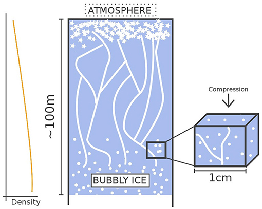
Figure 1. Scheme of a firn column with a decreasing porosity with depth (white inclusions in the firn) until it transforms into airtight ice. The scheme shows the transformation of the open porosity (long connected white channels) into closed bubbles. This paper focuses in modeling small scale firn samples originating from the bubble closure zone in deep firn, similarly to the zoomed box on the right side.

2.1. General Principles

This section aims to describe the general principles behind our 3D model, independent of their specific numerical implementation. First, we describe the two physical mechanisms taken into account in the model, namely the ice dislocation creep and surface curvature-driven diffusion. Note that other mechanisms, such as the sublimation and deposition of water molecules with transport through the pore phase (Calonne et al., 2014) could be added in the future. We then present the Level-Set method, that is used to represent the position of the ice/pore interface in the model.

2.1.1. Ice Dislocation Creep

The first physical mechanism taken into account for the deformation of the porous network is the dislocation creep of the ice phase, due to the compression forces of the firn column above (Wilkinson and Ashby, 1975; Arzt et al., 1983). In the model we consider that the ice matrix can be represented as polycrystalline ice, neglecting the influence of individual crystallographic grains. The creep deformation of the ice is a viscoplastic motion with a low Reynolds number. The equations governing the motion of the ice matrix are the Stokes equations:

$\begin{array}{ll}\begin{array}{c}\nabla ·\stackrel{-}{\stackrel{-}{\sigma }}+{\rho }_{\text{ice}}\mathbf{\text{g}}=0\\ \nabla ·{\mathbf{\text{v}}}^{\text{c}}=0\end{array}& (1)\end{array}$

where ∇· is the divergence operator, $\stackrel{-}{\stackrel{-}{\sigma }}$ is the stress tensor, ρ_ice is the density of ice, g is the gravity acceleration vector, and v^c is the ice creep velocity. To fully characterize the deformation of the ice matrix, the Stokes equations have to be completed with a constitutive law, describing the rheology of the ice material. Here, the creep of ice is represented by a Norton-Hoff power law (also referred to as Glen's law in glaciology; Duval et al., 1983; Schulson and Duval, 2009; Cuffey and Paterson, 2010):

$\begin{array}{ll}{\stackrel{.}{ϵ}}_{ij}=A{\tau }^{n-1}{\sigma }_{ij}^{\prime }& (2)\end{array}$

where i and j represent Cartesian coordinates (x, y, or z), ${\stackrel{.}{ϵ}}_{ij}=\frac{1}{2}(\frac{\partial v_{\text{i}}^{\text{c}}}{\partial x_{\text{j}}}+\frac{\partial v_{\text{j}}^{\text{c}}}{\partial x_{\text{i}}})$ is the strain rate tensor ($v_{\text{i}}^{\text{c}}$ being a Cartesian component of the creep velocity), ${\sigma }_{ij}^{\prime }={\sigma }_{ij}-1/3\text{Tr}(\sigma ){\delta }_{ij}$ is the deviatoric stress tensor, with σ_ij being a component of the stress tensor $\stackrel{-}{\stackrel{-}{\sigma }}$ and δ_ij the Kronecker delta, and ${\tau }^2=\frac{1}{2}{\sigma }_{ij}^{\prime }{\sigma }_{ij}^{\prime }$ is the effective shear stress. The parameter n is set to 3 (Schulson and Duval, 2009; Cuffey and Paterson, 2010). For the rest of the article, the pre-factor A is set to 0.08MPa⁻ⁿ yr⁻¹ which is the expected value for ice around the −50°C temperature. However, the model could be run at other temperatures by taking into account the documented dependence of A to temperature (Schulson and Duval, 2009; Cuffey and Paterson, 2010).

2.1.2. Surface Diffusion

The second mechanism implemented in the model is the diffusion of ice molecules due to gradients of chemical potential created by local curvature conditions. There are several mechanisms for the diffusion of water molecules as a response to these curvature differences (Ashby, 1974; Maeno and Ebinuma, 1983). Diffusive mechanisms transport mass from regions of high curvature toward regions of low curvature. As it has already been successfully implemented in Level-Set simulations (Bruchon et al., 2010, 2012), we implemented the specific mechanism of surface diffusion in which water molecules diffuse at the surface of the ice/pore interface. Following the work of Bruchon et al. (2010) and Bruchon et al. (2012), the equation governing the velocity of the interface is:

$\begin{array}{ll}{\mathbf{\text{v}}}^{\text{d}}=-C_0({△}_{s}K)\mathbf{\text{n}}& (3)\end{array}$

with C₀ being a parameter representing the effectiveness of the diffusive mechanism, K the curvature of the interface, n the normal vector to the interface pointing in the ice phase, and Δ_s is the “surface Laplacian” (the Laplace-Beltrami operator).

The value of the parameter C₀ governing surface diffusion depends on the thickness in which diffusion occurs, the free energy of the ice surface, and the diffusion coefficient of water molecules at the ice surface (Bruchon et al., 2010). Unfortunately, these quantities are not well constrained, leading to a large uncertainty on the value of C₀ and its dependence to temperature (Petrenko and Whitworth, 1999). To overcome this issue, we evaluated that the mechanism of diffusion results in interface velocities similar to ice creep for $C_0\simeq 10^{-6}$ mm⁴ yr⁻¹. Therefore, in the rest of the study the parameter C₀ will be set to the values 10⁻⁶ or 10⁻⁷ mm⁴ yr⁻¹ to, respectively represent the presence of a strong or mild influence of the diffusion process, relatively to ice creep.

Finally, as the mechanism of surface diffusion redistributes mass from some regions to others, it is mass conserving and does not modify the density of firn layers. A mathematical proof of this mass conservation, involving the generalized divergence theorem over closed surfaces, is presented in Bruchon et al. (2010).

2.1.3. The Level-Set Method

The goal of this model is to explicitly simulate the evolution of the ice/pore interface in firn. This evolution notably includes topological changes, resulting from pore closure or coalescence (Burr et al., 2019). In the model, the bi-phasic nature of the firn is replaced by a mono-phasic medium with the addition of a characteristic function retaining the position of the ice/pore interface, the so called Level-Set (LS) function ϕ (Osher and Sethian, 1988; Gibou et al., 2018). This Level-Set framework naturally handles topological changes, which is needed to model the closure or coalescence of pores (Osher and Sethian, 1988). A typical choice for the LS function is the signed distance to the interface.

Considering a 3D domain D of firn the LS function ϕ is given by:

$\begin{array}{ll}\varphi (x)=\{\begin{array}{c}+\text{dist}(x,\Sigma )\text{ if }x\in \text{ice}\\ -\text{dist}(x,\Sigma )\text{ if }x\in \text{pore}\\ 0\text{ if }x\in \Sigma \end{array}& (4)\end{array}$

where x is a point of D, Σ is the interface between the ice and pore phases, and dist(x, Σ) is the distance of point x to the interface. The position of the interface is thus captured by the zero-level of the LS function, as one can retrieve it with Σ = {x∣ϕ(x) = 0}. The evolution of the porous network is therefore represented by the evolution of the zero-level of the LS function.

The velocity v^tot of the ice/pore interface is the sum of the velocities induced by each individual physical mechanism. This velocity is then used to advect the LS function by solving the transport equation (Olsson and Kreiss, 2005; Bernacki et al., 2008):

$\begin{array}{ll}\frac{\partial \varphi }{\partial t}+{\mathbf{\text{v}}}^{\text{tot}}·\nabla \varphi =0& (5)\end{array}$

2.2. Numerical Implementation

For our specific implementation, we rely on the Finite Element Method (FEM) to solve the equations involved in the model. The FEM allows us to use unstructured tetrahedral meshes, that can be adapted to the represent the 3D geometries of the ice and pore phases. In our case, we use first order tetrahedral elements.

Moreover, we rely on the open source Finite Element software Elmer¹ (Gagliardini et al., 2013), that notably provides a module to compute the deformation of the ice matrix, as well as a general framework to solve equations with the FEM. In Elmer, we use Biconjugate Gradient Stabilized iterative solvers, with the standard Incomplete LU factorization for preconditioning. When transient equations are used in Elmer, we rely on the Backward Difference Formula (second order) for time-stepping. Furthermore, in our implementation all vectorial equations are treated with 3D Cartesian coordinates.

To compute the evolution of the firn microstructure our model goes through three main stages at each time-step Δt: (i) the tetrahedral mesh is adapted to the firn microstructure given by the LS function, (ii) the interface velocities for each physical mechanisms are computed, (iii) the LS function is advected to represent the movement of the interface. The overall algorithm, with the mesh adaptation, computation of velocities, advection steps, as well as the initialization of the model, is summarized in Figure 2.

FIGURE 2

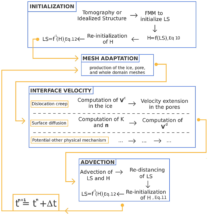
Figure 2. Scheme of the model algorithm. Each blue box represents a core stage of the simulation.

2.2.1. Mesh Adaptation

The mesh is adapted to the LS function at the beginning of each time-step. The first goal of the mesh adaptation is to improve the computational efficiency of the model by keeping a refined mesh near the ice/pore interface and a coarser resolution away, where a high density of elements is not needed (Olsson et al., 2007; Bruchon et al., 2010). The second goal is to produce two sub-meshes, referred to as ${{M}}_{\text{i}}$ and ${{M}}_{\text{p}}$. The first one is meant to cover the ice phase only, and the second one the pore phase only. Note that an equivalent model could have been developed using passive elements instead of producing the sub-meshes ${{M}}_i$ and ${{M}}_p$. However, we chose the latter method as it simplifies the visualization of the results.

At the end of the nth time-step, the LS function is defined on a tetrahedral mesh ${{M}}_D^n$ covering the whole domain. Its zero-value level gives the position of the ice/pore interface for the following time-step. At the start of the new time-step, the mesh adaptation procedure produces three meshes ${{M}}_D^{n+1}$, ${{M}}_i^{n+1}$, and ${{M}}_p^{n+1}$ that cover the whole domain, the ice phase and the pore phase. The ice mesh is composed of the elements of ${{M}}_D^{n+1}$ that lie in the ice phase region, and similarly for the pore mesh. The vertices of ${{M}}_i^{n+1}$ and ${{M}}_p^{n+1}$ are thus also vertices of ${{M}}_D^{n+1}$. Mathematically, ${{M}}_D^{n+1}$ is thus the union of ${{M}}_i^{n+1}$ and ${{M}}_p^{n+1}$, while the intersection of ${{M}}_i^{n+1}$ and ${{M}}_p^{n+1}$ defines the ice/pore interface.

To mesh the domain according to the LS function, we rely on the remeshing library MMG² (based on Dapogny et al., 2014), that we have interfaced with Elmer. The library yields a tetrahedral mesh that is refined around the ice/pore interface, with tetrahedral elements either in the ice or pore phase, and tagged accordingly. The boundaries between the elements of the ice and pore regions thus lie on the zero-value level of the LS function. The MMG library includes parameters to adjust the mesh refinement. The main ones are the h_grad and h_ausd parameters, that respectively set the gradation of element sizes and the maximal distance between the ideal interface (defined by the LS function) and the interface captured by the tetrahedral mesh.

The mesh obtained with the MMG library is used as the domain mesh ${{M}}_D^{n+1}$. Furthermore, the sub-meshes ${{M}}_i^{n+1}$ and ${{M}}_p^{n+1}$ are derived using the element-tag provided by the MMG library. The different variables defined at the nodes of ${{M}}_D^n$ are finally interpolated on the new nodes of ${{M}}_D^{n+1}$. This includes the LS function.

In order to facilitate the transfer of variables between the ${{M}}_D^{n+1}$, ${{M}}_i^{n+1}$, and ${{M}}_p^{n+1}$ meshes, permutations tables that link a vertex in ${{M}}_D^{n+1}$ to its equivalent in ${{M}}_i^{n+1}$ and/or ${{M}}_p^{n+1}$ are saved under the form of two arrays of integers. For a given node of index i in the domain mesh, the ith value of the permutation table is the index of the corresponding node in the ice mesh (respectively pore mesh) or 0 if the node does not lie in the ice phase (respectively pore phase). This allows to transfer variables from one mesh to another without interpolation, and with a good numerical efficiency. The complete mesh adaptation step procedure is summarized in Figure 3.

FIGURE 3

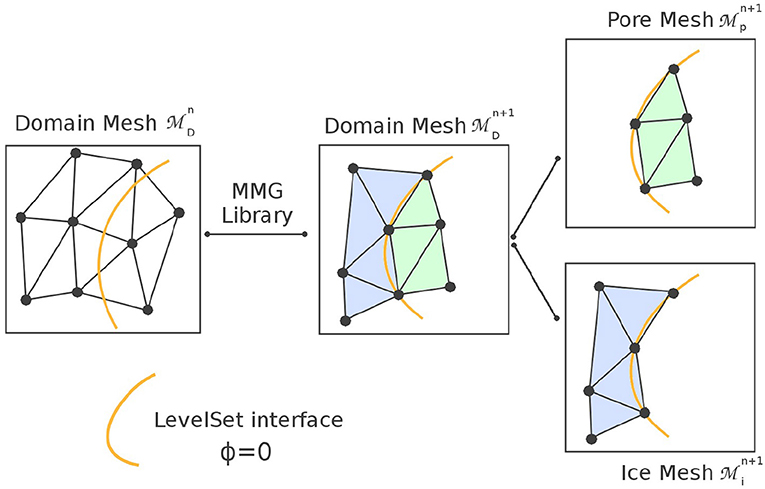
Figure 3. Mesh adaptation of the domain following the LS function. The submeshes of the ice and pore phases ${{M}}_i$, and ${{M}}_p$ are also produced during mesh adaptation.

2.2.2. Computation of the Ice Creep Velocity

To compute the deformation of the ice matrix a numerical oedometric compression is performed, where the ice is compressed at the top and retained on all other sides. The enforced boundary conditions are therefore ones of non-penetration on all the domain sides (v^c · n = 0, where n is the normal vector to the boundary), except for the top side where a normal stress is enforced on the ice ($\stackrel{-}{\stackrel{-}{\sigma }}\mathbf{\text{n}}=-P\mathbf{\text{n}}$, where P is the pressure imposed by the overlying column and the atmosphere). This overburden pressure increases with time according to the accumulation rate. The difference between high and low accumulation sites can therefore be modeled with appropriate choices for the increase of the overburden pressure over time. Finally, the force exerted by the air pressure in the pores is applied at the ice/pore interface. The Stokes equations are solved on the ice mesh ${{M}}_i$ using the module readily available in Elmer.

The output velocity field of this oedometric compression produces a lot of displacement at the top of domain and practically none at the bottom. This means that at the top of the domain, the LS function would have to be advected over a long distance during a single time-step, which is numerically detrimental as it increases the Courant number (Courant et al., 1967). In order not to have all the displacement concentrated in one zone, we subtracted its average vertical value to the oedometric ice creep velocity field. This results in a field with the same strain and thus the same deformation of the porous network, but with a vertical velocity field distributed between the top and bottom parts of the sample, as seen in the left panel of Figure 4. This distributed velocity field is the velocity used in the model for the creep movement of the ice matrix. Note that performing an oedometric compression and subtracting the average vertical velocity, is equivalent to enforcing a Dirichlet condition of null vertical velocity in the middle of the domain.

FIGURE 4

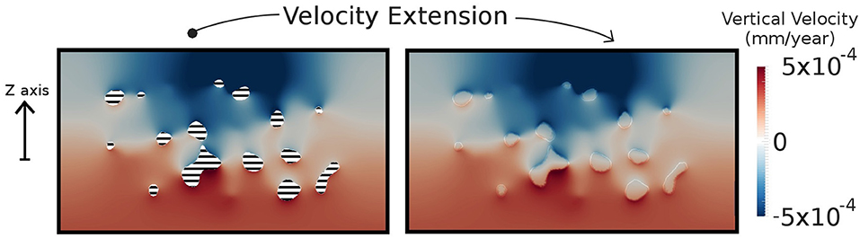
Figure 4. Cut-views of a 3D firn sample (~100 m deep, 7.57 × 3.75 mm dimensions). (Left) Vertical creep velocities computed in the ice phase. The pores are filled with black horizontal stripes. (Right) Vertical creep velocities extended to the whole domain.

After solving Equation (1) and subtracting the average vertical value, the creep velocities are known within the ice material. However, to advect the LS function it is necessary for the advection velocity field to be defined on each side of the interface, and thus also inside the pore phase. This is a classical problem of the Level-Set method that can be solved with the aid of velocity extension methods (Adalsteinsson and Sethian, 1999). Here, the ice velocity is extended to the pore phase by solving the Equation:

$\begin{array}{ll}-\alpha \Delta {\mathbf{\text{v}}}^{\text{ext}}+{\mathbf{\text{v}}}^{\text{ext}}=0& (6)\end{array}$

where Δ is the Laplace operator, v^ext the extended velocity, and α a smoothing parameter. The equation is solved on the pore mesh ${{M}}_p$, with the boundary condition setting the extended velocity equal to the dislocation creep velocity on the ice/pore interface. The solution of Equation (6) is a smooth velocity field, that is equal to the ice creep velocity at the ice/pore interface.

The creep velocity on the ice mesh, and the extended velocity on the pore mesh are then transferred to the domain mesh ${{M}}_D$. This results in a continuous velocity field defined on the whole domain D, that matches the ice creep in the ice region. An example of ice creep velocity extension is given in Figure 4.

2.2.3. Computation of the Surface Diffusion Velocity

To compute the surface diffusion velocity using Equation (3), one requires the curvature K and the normal vector n. They can be calculated using:

$\begin{array}{ll}\mathbf{\text{n}}=\frac{\nabla \varphi }{\Vert \nabla \varphi \Vert }& (7)\end{array}$

and

$\begin{array}{ll}K=-\nabla ·\mathbf{\text{n}}& (8)\end{array}$

However, Equations (3) and (8) require second-order derivatives, which are not easily computed using first order elements. To reduce numerical noise, Equations (3) and (8) are stabilized with the introduction of diffusion parameters A_k and A_v:

$\begin{array}{ll}\begin{array}{c}K+A_{\text{k}}\Delta K=-\nabla ·\mathbf{\text{n}}\\ v^{\text{d}}+A_{\text{v}}\Delta v^{\text{d}}=C_0({\Delta }_{\text{s}}K)\end{array}& (9)\end{array}$

where v^d is the norm of v^d.

To compute the diffusion velocity vector v^d, the normal vector n is first computed using Equation (7). The curvature K is then computed by solving the first equation of Equations (9). The norm v^d of v^d is computed by solving the second equation of Equations (9). The vector v^d is finally obtained by applying the norm v^d to the direction supported by n. These computations are performed using Elmer modules specifically developed for this firn model.

2.2.4. Advection of the Level-Set

Once the total velocity of the interface (the sum of the creep and diffusion velocities) is computed, it is used to modify the porous structure of the firn material by advecting the LS function. However, the sole advection of the LS function using the velocity field is not sufficient to ensure a good representation of the evolution of the interface. Indeed, the property of the LS function to be a signed distance function is lost during the advection step, although it is fundamental for the computation of normal vectors and curvatures (Equation 7 for instance). That is why the LS function is regularly re-distanced, meaning that it is recomputed to remain a signed distance (Osher and Fedkiw, 2001). However, the re-distancing introduces errors and numerical diffusion in the model, that results in unphysical gain or loss of volume (Olsson and Kreiss, 2005). To overcome this issue, Zhao et al. (2014a) introduced the Improved Conservative Level-Set (ICLS) method following the work of Olsson et al. (2007) on the Conservative Level-Set method. To ensure volume conservation, we have implemented the ICLS method for the advection stage.

The ICLS method introduces a new scalar field H, similar to the LS function ϕ, defined as:

$\begin{array}{ll}H=\frac{1}{2}(1+\text{tanh}(\frac{\varphi }{2ϵ}))& (10)\end{array}$

It is a smeared Heaviside function, with a width of the order of ϵ. Similarly to the LS function, H captures the position of the ice/pore interface, that is located at H = 1/2. Moreover, H can also be used to compute the normal vector to the interface using Equation (7).

The implementation of the ICLS method works as follows. The LS and H functions are both advected on the mesh ${{M}}_D$ using the total interface velocity. The advection is performed using the Advect software³. The LS function is then re-distanced to remain a signed distance function, using the mshdist software⁴ (based on Dapogny and Frey, 2012). Next, the normal vectors to the new interface are computed. Near the interface the normal vector n is computed using the H function, and far from it is computed using the re-distanced LS function. This choice was made because using the H function to compute the normal vectors far from the interface yields spurious oscillations, a problem that does not arise with the LS function (Zhao et al., 2014a,b; Zhao L.-H. et al., 2014). A point of the domain is considered to be in the vicinity of the interface if its distance to the interface is smaller than twice the parameter ϵ in Equation (10). Then, the shape and the width of the H function are maintained thanks to a re-initialization step (Olsson et al., 2007; Zhao et al., 2014a,b; Zhao L.-H. et al., 2014). It consists in solving the equation:

$\begin{array}{ll}\frac{\partial H}{\partial T}+\nabla ·\left[H(1-H)\mathbf{\text{n}}\right]=\nabla ·\left[ϵ(\nabla H.\mathbf{\text{n}})\mathbf{\text{n}}\right]& (11)\end{array}$

In this equation, T is non-dimensionalized fictional time, distinct from the actual time, that is solely used to relax the equation to equilibrium (Olsson et al., 2007). The term on the left-hand side of Equation (11) compresses the width of the H function, while the right-hand side term expands it. The equation should be solved until the two terms balance, and a steady-state is reached (Olsson et al., 2007; Zhao et al., 2014a,b; Zhao L.-H. et al., 2014). In our model, the fictional time-step is set ΔT = 1, and the equation is solved for a total 15 fictional time-steps, which is enough to reach a steady state (Olsson et al., 2007). Once the H function has been re-initialized, the LS function ϕ is updated in the vicinity of the interface using:

$\begin{array}{ll}\varphi =2ϵ\text{ tan}{\text{h}}^{-1}(2H-1)& (12)\end{array}$

The advection step is then finished and the LS function defines the interface for the following time-step.

2.2.5. Initialization of the Model

The model needs to be initialized with a LS function, representing either a real firn porous structure or an idealized geometry. The initial porous structure can be derived from 3D voxel models obtained with Xray tomography of firn samples (Barnola et al., 2004; Gregory et al., 2014; Burr et al., 2018). To simplify the boundary conditions, the tomography models are padded with ice material on all sides, meaning that the ice/pore interface lies away from the boundaries of the domain D.

Starting from a 3D voxel model, the signed distance is computed on a Cartesian grid using the Fast Marching Method (FMM; Sethian, 1999). It is performed using the scikit-fmm⁵ python package. The signed distance is then smoothed using a gaussian filter to remove the jags of the interface. The resulting signed distance defines the initial LS function, and is interpolated on the initial mesh ${{M}}_D^0$. Since, the position of the ice/pore interface is not known in advance, ${{M}}_D^0$ is finely resolved over the whole domain to properly capture its initial position.

Next, the H function is determined using Equation (10). In order to further smooth the interface and remove remaining jags, we perform a re-initialization step of H solving Equation (11) to equilibrium, followed by a LS function update using Equation (12). At this stage, the simulation can start with a mesh adaptation step.

3. Numerical Experiments

In this part we present a few numerical experiments, performed with the 3D firn model presented before. The aim of section 3.1 is to assess the capability of our model to conserve mass thank to the ICLS method. In section 3.2, we then use the model to quantify the impact of building pressure on the compressibility of closed pores in deep firn. Finally, section 3.3 discusses the contribution of individual physical mechanisms to the splitting of pores.

3.1. Mass Conservation

The goal of the ICLS method (Equation 11) and of the re-initialization is to ensure mass and volume conservation (Olsson et al., 2007; Zhao et al., 2014a,b; Zhao L.-H. et al., 2014). Similarly to Zhao et al. (2014b), we test the mass conservation of our micro-mechanical model by considering the advection of an idealized structure, in our case a sphere.

The domain is composed of a column of ice with dimensions 1 × 1 × 4 mm. The LS function is initialized to represent a spherical pore of radius 0.25 mm at the bottom of the column (see the left panel of Figure 5). This sphere is advected upward with a constant velocity of 10⁻³ mm yr⁻¹. Note that this advection velocity is imposed and does not depend on the computation of the mechanisms of surface diffusion or ice dislocation creep. Pictures of the sphere at the beginning and the end of the simulation are shown in Figure 5. The volume of the sphere is computed at the end of each time-step using the volume enclosed by the LS function.

FIGURE 5

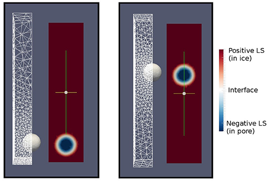
Figure 5. Advection of a sphere. The left and right panels, respectively display the start and end the simulation. In each panel: the left part is the side view of the structure with the surface of the sphere in gray and the mesh of the exterior ice in white. The right part is a cross section of the column showing the LS function. Red colors represent the ice phase and blue colors the pore phase.

With several sets of parameters, we tested the influence of the h_grad (mesh size gradation), h_ausd (controlling the mesh size at the interface), and ϵ (width of the H function) parameters on mass conservation. The different parameters of the simulations are listed in Table 1. The volume error evolutions are displayed in Figure 6. In the two best experiments (Exp2 and Exp7), the volume error does not exceed 2.5% after 20 time-steps and a total displacement of the sphere of 2 mm. These two cases are represented as orange pentagons and gray rhombuses in both panels of Figure 6. The results of the experiments show that smaller time-steps do not necessarily imply a better mass conservation. Indeed, comparing the blue dots (Δt = 100 yr, Exp1) and the yellow crosses (Δt = 50 yr, Exp8) points in Figure 6 indicates a larger error at the end of the total advection in the case of the smaller time-step. Our understanding is that each time-step introduces volume errors during the advection step, and that multiplying time-steps accumulates the errors.

TABLE 1

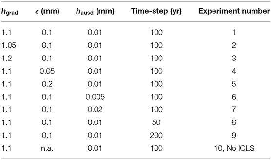
Table 1. Parameters used for the sensitivity test of mass conservation.

FIGURE 6

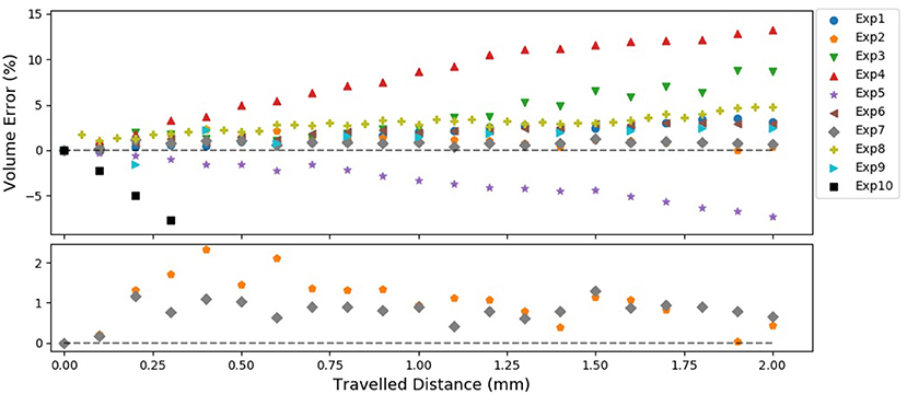
Figure 6. Volume error of the advected sphere, expressed in percent of its initial volume. The orange pentagons and gray rhombuses correspond to the best parameterizations for mass conservation, and the black squares to an advection experiment without the ICLS method. The specific parameters of the other simulations are given in Table 1. The lower panel is a zoom to the best simulation results.

Moreover, it appears that a poor choice of parameters can lead to an important accumulation of errors over time, as seen with Exp3, 4, and 5 in Figure 6. It is however not straightforward to estimate the ideal parameters for a given simulation, as they depend on the specific geometry and velocity field of the problem. To limit problems of mass conservation, the rest of the simulations of this paper will not be run for more than 10 time-steps. Figure 6 indicates that this should result in total errors of <5%. In contrast, a simulation without the ICLS results in a ~10% volume error after three time steps (black squares in Figure 6). This experiment highlights the necessity of the ICLS method to maintain small volume errors. For the rest of the article, the mesh adaptation parameters are set to h_ausd = 0.01 mm, h_grad = 1.15, and ϵ = 0.1 mm. This results in boundary triangle elements with an average side of about 0.06 mm.

Zhao et al. (2014b) report a similar mass conservation experiment for a 2D case using an advected circle. They manage to maintain a relative error below 2%, for a total advection of about 250 diameters of the circle. Even though the 3D and 2D cases cannot be directly compared, it suggests that the model could be improved to obtain a better mass conservation. Moreover, there is a broad scientific literature on the implementation of conservative advection schemes for the Level-Set method (e.g., Kees et al., 2011; Owkes and Desjardins, 2013; Chiodi and Desjardins, 2017), that could benefit to the mass conservation capacity of our model in the future.

3.2. Effect of Internal Pressure on Pore Compression

As a first application of the model, we quantify the impact of internal pressure on the compression of closed pores. Indeed, current gas trapping models assume that in deep firn, open, and already closed pores compress in a similar fashion (Rommelaere et al., 1997; Buizert et al., 2012; Witrant et al., 2012). In real firn, the increased pressure in the already closed bubbles might slow their compression compared to open pores. A recent study by Fourteau et al. (2019) has shown that reducing the compressibility of closed pores by an amount of 50% in gas trapping models could explain a discrepancy between model results and direct measurements of air content in ice cores. It is however not clear if this reduced compressibility of 50% is physically sound or not.

To answer this question, we simulate the densification of a layer of the Lock-In firn, on the East Antarctic plateau. This site is characterized by an accumulation rate of 3.9 cm yr⁻¹ (ice equivalent), a surface temperature of −53°C, and a surface pressure evaluated at 0.0645 MPa (645 mbar) (Fourteau et al., 2019). The model is initialized with the microstructure obtained with a 2.5 × 2.5 × 2.5 mm tomography image, and selected at 80 m depth, near the start of the pore closure zone.

Two distinct simulations are performed. In the first one, the internal pressure of the pores is set to 0.065 MPa, the pressure of open pores found ~100 m below surface. This thus corresponds to the compression of open pores. In the second case, the internal pressure of the pores increases according to its reduction of volume, following an ideal gas law. This represents the compression of closed pores. In both cases, the compression forces of the overlying column start at 0.62 MPa and increases over time due to the surface accumulation rate of 3.9 cm of ice equivalent per year. Furthermore, the mechanism of surface-diffusion is removed from the simulations. As this mechanism does not theoretically modify the total volume of the porosity, it should not influence the effect of pore pressure on their compressibility. The time-step is set to 200 yr, which results in a maximum displacement of the interface that does not exceed a few percents of the characteristic size of the pores.

The relative volume evolutions of the pores for 10 time-steps are displayed in Figure 7. The volume variations are larger than the uncertainties reported in section 3.1, and cannot be explained solely by mass conservation errors. It appears that the effect of building pressure does not have a strong impact on pore volume until more than 500 years have passed. At that point, the building pressure in the closed pores reaches 0.16 MPa, more than twice the initial value. The measured thickness of the pore closure zone at Lock-In is of about 20 m (Fourteau et al., 2019). With an accumulation of 3.9 cm per year, a given firn stratum takes about 500 yr to cross the pore closure zone. Therefore, this simulation suggests that the effect of building pressure in closed bubbles does not play a major role in the pore closure zone.

FIGURE 7

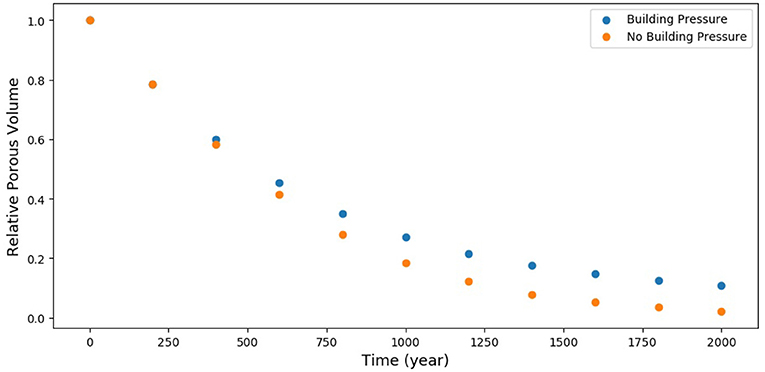
Figure 7. Relative volume as a function of time, with or without building of internal pressure.

To better quantify this effect, we computed the compression speed of the porosity in each case (building pressure and no pressure building cases). The compression speed is defined here as ∂_tV/V, where V is the volume of the porosity and ∂_tV is its temporal derivative. Figure 8 shows the reduction of compression speed due to the building of internal pressure, compared to the case with pressure kept constant. Within the pore closure zone (t ≤ 500 years), the compression speed with increasing pressure is reduced on average by 10%. The discrepancy between modeled and measured air content values in ice cores reported by Fourteau et al. (2019) cannot therefore be explained solely by the reduced compressibility of closed pores.

FIGURE 8

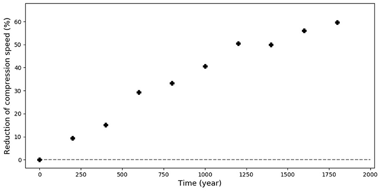
Figure 8. Reduction of the compression speed of closed pores due to the building of pressure. The dashed line represents a non reduced compression speed, as in the constant pressure case.

3.3. Contributions of Dislocation Creep and Surface Diffusion to Pore Splitting

In a recent article, Burr et al. (2019) performed different types of cold-room experiments to study the decoupled contributions of ice creep and curvature-driven diffusion to the evolution of firn and its porosity. They conclude that both compression and diffusive mechanisms contribute to the separation of pores.

In this section, we modeled the equivalent of Burr et al. (2019) experiments to study the individual contributions of dislocation creep and surface diffusion to the densification of firn and the closure of pores. In total, we run four different experiments, all initialized with the same porous network. The structure is extracted from the tomography image of a real firn sample excavated around the 100 m depth in the Lock-In firn core, described in the previous section. A 5.35 × 5.35 × 3.75 mm rectangular cuboid was extracted from a tomography image and used for initialization. The initial structure is shown in the left side of Figure 9. The compression imposed by the overlying firn column starts at 0.66 MPa and increases over time according to the 3.9 cm of ice per year accumulation rate. The internal pressure of the pores is maintained at 0.065 MPa, as we have seen that the building pressure in closed pores is small in the pore closure zone. All simulations are performed with a 100 years time-step, for a maximum of 10 time-steps.

FIGURE 9

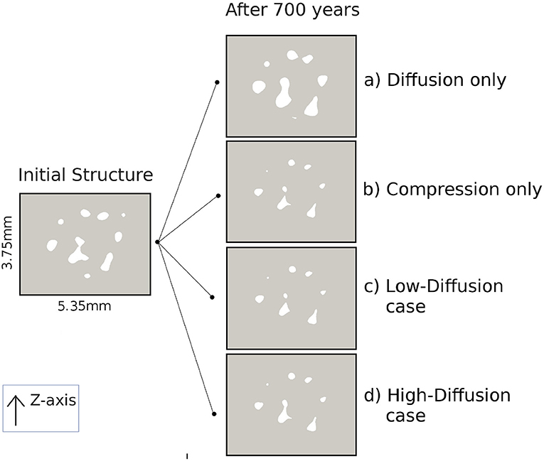
Figure 9. 2D cut-views of the firn material. The gray medium is the ice matrix, and the white spaces are the pores. The slice on the left shows the initial porous structure used in all the simulations, and the four slices on the right show the results of the four different simulations after 700 years. (A) Diffusion only, (B) compression only, (C) Low-diffusion case, (D) High-diffusion case.

3.3.1. Surface Diffusion Only

In the first simulation, the process of ice creep is removed and only the curvature-driven surface diffusion is taken into account. The parameter C₀ is set to 10⁻⁶ mm⁴ yr⁻¹. The evolution of the initial firn structure after 700 years of evolution with surface diffusion only is displayed in Figure 9A. As seen in the figure, the mechanism of surface diffusion leads to a rounding of pores over time. This is consistent with a mass transport occurring from regions of high curvature toward regions of low curvature, as exemplified in Figure 10. While Burr et al. (2019) report that letting firn samples evolve at rest in a relatively high-temperature environment (−2°C) without compression leads to pore splitting, we did not observe such phenomenon in our simulation.

FIGURE 10

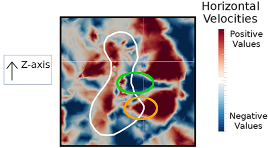
Figure 10. 2D cut-view of the firn material showing the surface-diffusion velocity field in the horizontal direction. Blue colors stand for negative values and red colors for positive values. The interface of a pore is highlighted in white in the middle of the section. The green and orange circles, respectively, show the regions where the interface is receding in the ice phase and growing in the pore phase. This leads to the rounding of the pore.

As the LS function gives the position of the ice/pore interface, it is possible to convert the output of the simulation into binary images, similar to tomographic images. We performed this conversion for the time-steps t = 0 and t = 700 years. The binary images can then be analyzed as tomographic images, and the number of individual pores in the medium can be counted (using the ImageJ plug-in Analysis_3D here; Boulos et al., 2012). It reveals that the simulation starts with 39 individual pores in the volume and drops to only 9 individual pores after 700 years. This highlights that pore coalescence happened multiple times during the simulation. Thanks to the LS function, the density of the medium during the simulation can be quantified. The initial ice volume fraction is 0.902, and drops to 0.884 after 700 years, that is to say a decrease of about 2%. However, the mechanism of surface diffusion should theoretically not modify the density of the medium (Bruchon et al., 2010). This drop in ice volume fraction could be explained by the insufficient mass conservation of the model, as it is of the order of the volume error reported in section 3.1. Furthermore, a closer look at the surface diffusion velocity field in Figure 10, indicates that despite the stabilization of the equations (introduced in Equations 9) the velocity field exhibits a lot of variability that is likely related to numerical noise, rather than physically-relevant variability. We might therefore expect our representation of surface diffusion to introduce some numerical noise in the results, which could also contribute to the decrease in density.

3.3.2. Ice Creep Only

The second simulation is performed with solely the mechanism of ice creep. The evolution of the initial structure after compression is displayed in Figure 9B. As seen in the figure, this simulation leads to a densification of the medium, with a smaller porous network. This observation is confirmed by the analysis of the ice volume fraction, that increased from 0.902 to 0.960 after 700 years. This increase is larger than the uncertainties reported in section 3.1, and cannot therefore be solely explained by a mass conservation problem.

The simulation also visually exhibits pore splitting. This is confirmed by counting the number of individual pores before and after the compression. This number increased from 39 to 57 pores, showing the ability of the ice creep mechanism to split and isolate pores from the atmosphere. The same observation of pore splitting was made by Burr et al. (2019). They report pore separations of a sample during ongoing densification that is subject to solely mechanical loading.

3.3.3. Combined Ice Creep and Surface Diffusion

The third and fourth simulations take into account the combined effects of curvature-driven surface diffusion and ice creep. The parameter C₀ is set to values of 10⁻⁶ and 10⁻⁷ mm⁴ yr⁻¹, to represent different levels of curvature-driven diffusion, respectively referred to as the high-diffusion and low-diffusion cases for the rest of the section.

2D cut-views of both simulations after 700 years are displayed in Figure 9C (low-diffusion case) and Figure 9D (high-diffusion case) in the right side of Figure 9. The results show an increase in ice volume fraction from 0.902 to 0.959 for the low-diffusion case, and to 0.953 for the high-diffusion case. Increasing the role of diffusion in the simulation leads to a slightly smaller density. This is consistent with the 0.960 value reported in the absence of surface diffusion. Moreover, observation of the Lock-In firn core shows that ice volume fractions of 0.95 are found around the 130 m depth. This is consistent with the 700 years sinking time of the simulation, which corresponds to about 30 m of depth increase.

Analysis of the results also shows an increase in the number of individual pores from 39 to 61 and 50 for the low and high-diffusion, respectively. It appears that in the high-diffusion case, the mechanism of surface diffusion slows down the splitting of pores. Our understanding is that the diffusive mechanism leads to a rounding of the pores, preventing the development of small necks that would eventually lead to pore splitting. Surprisingly, the low-diffusion case displays a little more pore splitting than the case without any surface diffusion, that resulted in 57 individual pores after 700 years. It is not clear if this is related to a specific inter-play between the diffusion and creep mechanisms that would accelerate the splitting of pores, or simply numerical noise.

4. Discussion

Combining the Finite Element and Level-Set methods is a promising modeling approach to simulate the topological evolution of firn under compression. Notably, the use of a mesh for the ice phase enables to easily compute deformation velocities as response to mechanical compression. This velocity field can then be used to simulate the evolution of the ice/pore interface with the LS function.

Yet, several optimizations and improvements of the model are still required before its operational application to study the closure of pores in polar firn. First, the model is currently fully sequential. Running a 10 steps simulation on a single processor and for a 5.35 × 5.35 × 3.75 mm firn sample requires roughly a day of computation. The parallelization of the model would curb down this time, and allow to use the model on several-centimeter large domains, which have been shown to be more representative of real firn (Schaller et al., 2017; Burr et al., 2018). Moreover, parallelization would allow to use finer meshes and more complex numerical schemes that could improve the mass conservation and numerical stability of the model. The current version of the model cannot indeed ensure a mass conservation better than about 5% after ten time steps. This limits the ability of the model to perform simulations covering large time periods, and to accurately quantify the density increase of firn samples. Future work on the model should improve this mass conservation problem, potentially with the use of other mass-conserving advection schemes from the literature (e.g., Kees et al., 2011; Owkes and Desjardins, 2013; Chiodi and Desjardins, 2017). Finally, as shown in section 3.3.1, the current implementation of the surface diffusion mechanism leads to a noisy velocity field that might deteriorate the robustness of the results. The use of a very fine mesh near the interface could help resolve this problem, but would lead to a sharp increase in the computation time. On the other hand, the use of more sophisticated stabilization techniques (such as in Bruchon et al., 2010) could resolve this issue without an additional computational cost. Another solution could be the use of second-order elements for the computation of the second-derivatives required for the diffusive mechanism. As diffusion appears to play a significant role in the morphology of pores (Burr et al., 2019), it seems important to implement a fast and robust representation of diffusive mechanisms in the model. This would help to decipher the relative contributions of ice creep and diffusion to the evolution of the porous network, and provide insights on the evolution of pores at very low temperature.

In the article we first use our model to assess the impact of internal building pressure on the compressibility of closed pores. This allows to test the proposed hypothesis of Fourteau et al. (2019) that a lower compressibility of closed pores could explain a discrepancy between modeled and measured air content values in ice cores. Our results indicate that the compressiblity of closed pores is only reduced by an amount of ~10%, much lower than the reduction needed to fully explain the model/data mismatch of Fourteau et al. (2019). Other potential mechanisms advanced by Fourteau et al. (2019) to explain this discrepancy are the brittle reopening of pores under pressure or the effusion of gases trough small capillaries not visible with Xray tomography or pycnometry measurements. Further work on the physical processes at play at the microstructural scale in firn is needed to resolve this question.

Then, we compare results of the model with cold-room experiments performed by Burr et al. (2019). While they report that both diffusive mechanisms and ice dislocation creep contribute to the separation of pores, we did not observe such a phenomenon in the simulations. In the model, the creep of the ice matrix leads to the separation of pores, but on the other hand the mechanism of surface diffusion leads to the rounding and even coalescence of pores. As seen in Figure 10, the surface diffusion velocity field exhibits numerical noise. This noise might lead to an unphysical movement of the ice/pore interface in the model, explaining some of the discrepancy with the experiment of Burr et al. (2019). However, we expect the mechanism of surface diffusion to transport mass from zones of high curvature to zones of low curvature. This would lead to the rounding of the pores, rather than the pore separation observed by Burr et al. (2019). Another potential explanation could be that the mechanism of surface diffusion implemented in the model is not representative of the diffusive mechanisms at play during (Burr et al., 2019) experiments. It is indeed possible that the dominant diffusive mechanism is the sublimation and redeposition of water molecules at the ice/pore interface, rather than the surface diffusion implemented in our model (Maeno and Ebinuma, 1983). However, the diffusion of water molecules through sublimation and redeposition would also transport matter from regions of higher curvature to regions of lower curvature. We might therefore also expect a rounding of the pores, hindering the formation of necks and their separation.

5. Conclusion

This article presents the development and implementation of a 3D micro-mechanical model of firn compression. In order to handle the topological changes occurring in the porous network of deep firn (such as pore splitting or pore coalescence) the model relies on the Level-Set framework to represent the position of the ice/pore interface. The model is able to determine the movement of the interface due to the creep of the ice matrix as a response to the mechanical stress imposed by the overlying firn column. Moreover, mechanisms of curvature-driven diffusion (in our case surface diffusion) can be added to the model. Finally, we implemented the Improved Conservative Level-Set Method (ICLS, Zhao et al., 2014a,b; Zhao L.-H. et al., 2014) to improve the mass conservation properties of the model. Numerical experiments on an idealized case indicate that the implementation of the ICLS method greatly improves the mass conservation. Yet, errors of several percent after ten time-steps are still present.

As a first application, we assess the impact of internal pressure in the compression of closed pores near the firn/ice transition. In order not to rely on an idealized geometry we used a real porous network, extracted from a tomographic image, to carry out the simulations. Our results indicate that the increase of internal pressure can be ignored at the bottom of the firn column, as assumed by existing gas trapping models (Rommelaere et al., 1997; Buizert et al., 2012; Witrant et al., 2012). Finally, we study the contributions of ice dislocation creep and surface diffusion to the densification of a small firn sample and to the separation of pores. As expected the mechanical compression of the firn sample leads to an increase in density, as well as pore splitting reflected by an increase in the number of individual pores. On the other hand, the mechanism of surface diffusion appears to lead to pore rounding which hinders their separation.

Our results suggest that the Level-Set method, combined with Finite Element modeling, can be adequate to study polar firn densification and pore isolation from the atmosphere, although several improvements are still required.

Data Availability Statement

The datasets generated for this study are available on request to the corresponding author.

Author Contributions

The model was developed by KF with the help of FG-C, following an idea of KF, PM, and XF. The manuscript was written by KF, with the help of all co-authors.

Funding

This work was supported by the French INSU/CNRS LEFE projects NEVE-CLIMAT and HEPIGANE. The Lock-In drilling operation was supported by the IPEV project no. 1153 and the European Community's Seventh Framework Programme under grant agreement no. 291062 (ERC ICE&LASERS). The tomography images were obtained by the Institute for Snow and Avalanche Research SLF (Davos, Switzerland).

Conflict of Interest

The authors declare that the research was conducted in the absence of any commercial or financial relationships that could be construed as a potential conflict of interest.

Acknowledgments

We thanks Christophe Martin and Didier Bouvard for pointing to us the usage of Level-Set models in the sintering community. We thank Maurine Montagnat for the useful discussion on ice mechanics. We thank Olivier Gagliardini for his help with the Elmer software. We thank Charles Dapogny for the useful discussion on the Level-Set method, mesh adaptation, and advection of scalar field. We thank Martin Schneebeli, Henning Löwe, and Anouk Marsal for their involvement with the tomography images. The Lock-In drilling operation was conducted by Phillipe Possenti, Jérôme Chappellaz, David Colin, Philippe Dordhain, and PM. We are thankful to MT and MR for reviewing this article, and to JG for editing it.

Footnotes

1. ^https://www.csc.fi/web/elmer/elmer

2. ^https://www.mmgtools.org

3. ^https://github.com/ISCDtoolbox/Advection

4. ^https://github.com/ISCDtoolbox/Mshdist

5. ^https://pypi.org/project/scikit-fmm/

References

Adalsteinsson, D., and Sethian, J. (1999). The fast construction of extension velocities in level set methods. J. Comput. Phys. 148, 2–22. doi: 10.1006/jcph.1998.6090

CrossRef Full Text | Google Scholar

Arnaud, L., Barnola, J.-M., and Duval, P. (2000). Physical modeling of the densification of snow/firn and ice in the upper part of polar ice sheets. Phys. Ice Core Rec. 285–305. Available online at: http://hdl.handle.net/2115/32472 (accessed March 06, 2020).

Google Scholar

Arthern, R. J., Vaughan, D. G., Rankin, A. M., Mulvaney, R., and Thomas, E. R. (2010). In situ measurements of antarctic snow compaction compared with predictions of models. J. Geophys. Res. Earth Surf. 115:F03011. doi: 10.1029/2009JF001306

CrossRef Full Text | Google Scholar

Arzt, E., Ashby, M. F., and Easterling, K. E. (1983). Practical applications of hot isostatic pressing diagrams: four case studies. Metall. Trans. A 14, 211–221. doi: 10.1007/BF02651618

CrossRef Full Text | Google Scholar

Ashby, M. (1974). A first report on sintering diagrams. Acta Metall. 22, 275–289. doi: 10.1016/0001-6160(74)90167-9

CrossRef Full Text | Google Scholar

Barnola, J.-M., Pierritz, R., Goujon, C., Duval, P., and Boller, E. (2004). 3D reconstruction of the vostok firn structure by x-ray tomography. Data Glaciol. Stud. 97, 80–84. Available online at: http://ftp.esrf.eu/pub/UserReports/21167_C.pdf (accessed March 06, 2020).

Google Scholar

Barnola, J.-M., Raynaud, D., Korotkevich, Y. S., and Lorius, C. (1987). Vostok ice core provides 160,000-year record of atmospheric CO₂. Nature 329, 408–414. doi: 10.1038/329408a0

CrossRef Full Text | Google Scholar

Bazin, L., Landais, A., Lemieux-Dudon, B., Toyé Mahamadou Kele, H., Veres, D., Parrenin, F., et al. (2013). An optimized multi-proxy, multi-site Antarctic ice and gas orbital chronology (AICC2012): 120-800 ka. Clim. Past 9, 1715–1731. doi: 10.5194/cp-9-1715-2013

CrossRef Full Text | Google Scholar

Bernacki, M., Chastel, Y., Coupez, T., and Logé, R. (2008). Level set framework for the numerical modelling of primary recrystallization in polycrystalline materials. Scr. Mater. 58, 1129–1132. doi: 10.1016/j.scriptamat.2008.02.016

CrossRef Full Text | Google Scholar

Bondzio, J. H., Seroussi, H., Morlighem, M., Kleiner, T., Rückamp, M., Humbert, A., et al. (2016). Modelling calving front dynamics using a level-set method: application to Jakobshavn Isbræ, West Greenland. Cryosphere 10, 497–510. doi: 10.5194/tc-10-497-2016

CrossRef Full Text | Google Scholar

Boulos, V., Fristot, V., Houzet, D., Salvo, L., and Lhuissier, P. (2012). “Investigating performance variations of an optimized GPU-ported granulometry algorithm,” in Proceedings of the 2012 Conference on Design and Architectures for Signal and Image Processing (Rhodes Island), 1–6.

Google Scholar

Bruchon, J., Drapier, S., and Valdivieso, F. (2010). 3D finite element simulation of the matter flow by surface diffusion using a level set method. Int. J. Numer. Methods Eng. 86, 845–861. doi: 10.1002/nme.3079

CrossRef Full Text | Google Scholar

Bruchon, J., Pino-Muñoz, D., Valdivieso, F., and Drapier, S. (2012). Finite element simulation of mass transport during sintering of a granular packing. Part I. Surface and lattice diffusions. J. Am. Ceram. Soc. 95, 2398–2405. doi: 10.1111/j.1551-2916.2012.05073.x

CrossRef Full Text | Google Scholar

Buizert, C., Martinerie, P., Petrenko, V. V., Severinghaus, J. P., Trudinger, C. M., Witrant, E., et al. (2012). Gas transport in firn: multiple-tracer characterisation and model intercomparison for NEEM, Northern Greenland. Atmos. Chem. Phys. 12, 4259–4277. doi: 10.5194/acp-12-4259-2012

CrossRef Full Text | Google Scholar

Burr, A., Ballot, C., Lhuissier, P., Martinerie, P., Martin, C. L., and Philip, A. (2018). Pore morphology of polar firn around closure revealed by X-ray tomography. Cryosphere 12, 2481–2500. doi: 10.5194/tc-12-2481-2018

CrossRef Full Text | Google Scholar

Burr, A., Lhuissier, P., Martin, C. L., and Philip, A. (2019). In situ X-ray tomography densification of firn: the role of mechanics and diffusion processes. Acta Mater. 167, 210–220. doi: 10.1016/j.actamat.2019.01.053

CrossRef Full Text | Google Scholar

Calonne, N., Geindreau, C., and Flin, F. (2014). Macroscopic modeling for heat and water vapor transfer in dry snow by homogenization. J. Phys. Chem. B 118, 13393–13403. doi: 10.1021/jp5052535

PubMed Abstract | CrossRef Full Text | Google Scholar

Chiodi, R., and Desjardins, O. (2017). A reformulation of the conservative level set reinitialization equation for accurate and robust simulation of complex multiphase flows. J. Comput. Phys. 343, 186–200. doi: 10.1016/j.jcp.2017.04.053

CrossRef Full Text | Google Scholar

Courant, R., Friedrichs, K., and Lewy, H. (1967). On the partial difference equations of mathematical physics. IBM J. Res. Dev. 11, 215–234. doi: 10.1147/rd.112.0215

CrossRef Full Text | Google Scholar

Cuffey, K., and Paterson, W. S. B. (2010). The Physics of Glaciers, 4th Edition. Academic Press. Available online at: https://www.elsevier.com/books/the-physics-of-glaciers/cuffey/978-0-12-369461-4

Google Scholar

Dansgaard, W. (1953). The abundance of O¹⁸ in atmospheric water and water vapour. Tellus A Dyn. Meteorol. Oceanogr. 5, 461–469. doi: 10.1111/j.2153-3490.1953.tb01076.x

CrossRef Full Text | Google Scholar

Dapogny, C., Dobrzynski, C., and Frey, P. (2014). Three-dimensional adaptive domain remeshing, implicit domain meshing, and applications to free and moving boundary problems. J. Comput. Phys. 262, 358–378. doi: 10.1016/j.jcp.2014.01.005

CrossRef Full Text | Google Scholar

Dapogny, C., and Frey, P. (2012). Computation of the signed distance function to a discrete contour on adapted triangulation. Calcolo 49, 193–219. doi: 10.1007/s10092-011-0051-z

CrossRef Full Text | Google Scholar

Duval, P., Ashby, M. F., and Anderman, I. (1983). Rate-controlling processes in the creep of polycrystalline ice. J. Phys. Chem. 87, 4066–4074. doi: 10.1021/j100244a014

CrossRef Full Text | Google Scholar

Fourteau, K., Faïn, X., Martinerie, P., Landais, A., Ekaykin, A. A., Lipenkov, V. Y., et al. (2017). Analytical constraints on layered gas trapping and smoothing of atmospheric variability in ice under low-accumulation conditions. Clim. Past 13, 1815–1830. doi: 10.5194/cp-13-1815-2017

CrossRef Full Text | Google Scholar

Fourteau, K., Martinerie, P., Faïn, X., Schaller, C. F., Tuckwell, R. J., Löwe, H., et al. (2019). Multi-tracer study of gas trapping in an East Antarctic ice core. Cryosphere 13, 3383–3403. doi: 10.5194/tc-13-3383-2019

CrossRef Full Text | Google Scholar

Gagliardini, O., Zwinger, T., Gillet-Chaulet, F., Durand, G., Favier, L., de Fleurian, B., et al. (2013). Capabilities and performance of Elmer/Ice, a new-generation ice sheet model. Geosci. Model Dev. 6, 1299–1318. doi: 10.5194/gmd-6-1299-2013

CrossRef Full Text | Google Scholar

Gibou, F., Fedkiw, R., and Osher, S. (2018). A review of level-set methods and some recent applications. J. Comput. Phys. 353, 82–109. doi: 10.1016/j.jcp.2017.10.006

CrossRef Full Text | Google Scholar

Goujon, C., Barnola, J.-M., and Ritz, C. (2003). Modeling the densification of polar firn including heat diffusion: application to close-off characteristics and gas isotopic fractionation for Antarctica and Greenland sites. J. Geophys. Res. Atmos. 108:4792. doi: 10.1029/2002JD003319

CrossRef Full Text | Google Scholar

Gregory, S. A., Albert, M. R., and Baker, I. (2014). Impact of physical properties and accumulation rate on pore close-off in layered firn. Cryosphere 8, 91–105. doi: 10.5194/tc-8-91-2014

CrossRef Full Text | Google Scholar

Herron, M. M., and Langway, C. C. (1980). Firn densification: an empirical model. J. Glaciol. 25, 373–385. doi: 10.1017/S0022143000015239

CrossRef Full Text | Google Scholar

Johnsen, S. J., Dansgaard, W., and White, J. (1989). The origin of Arctic precipitation under present and glacial conditions. Tellus B Chem. Phys. Meteorol. 41, 452–468. doi: 10.3402/tellusb.v41i4.15100

CrossRef Full Text | Google Scholar

Joos, F., and Spahni, R. (2008). Rates of change in natural and anthropogenic radiative forcing over the past 20,000 years. Proc. Natl. Acad. Sci. U.S.A. 105, 1425–1430. doi: 10.1073/pnas.0707386105

PubMed Abstract | CrossRef Full Text | Google Scholar

Kees, C., Akkerman, I., Farthing, M., and Bazilevs, Y. (2011). A conservative level set method suitable for variable-order approximations and unstructured meshes. J. Comput. Phys. 230, 4536–4558. doi: 10.1016/j.jcp.2011.02.030

CrossRef Full Text | Google Scholar

Loulergue, L., Schilt, A., Spahni, R., Masson-Delmotte, V., Blunier, T., Lemieux, B., et al. (2008). Orbital and millennial-scale features of atmospheric CH₄ over the past 800,000 years. Nature 453, 383–386. doi: 10.1038/nature06950

PubMed Abstract | CrossRef Full Text | Google Scholar

Lundin, J. M., Stevens, C. M., Arthern, R., Buizert, C., Orsi, A., Ligtenberg, S. R., et al. (2017). Firn model intercomparison experiment (FirnMICE). J. Glaciol. 63, 401–422. doi: 10.1017/jog.2016.114

CrossRef Full Text | Google Scholar

Lüthi, D., Floch, M. L., Bereiter, B., Blunier, T., Barnola, J.-M., Siegenthaler, U., et al. (2008). High-resolution carbon dioxide concentration record 650,000– 800,000years before present. Nature 453, 379–382. doi: 10.1038/nature06949

PubMed Abstract | CrossRef Full Text | Google Scholar

Maeno, N., and Ebinuma, T. (1983). Pressure sintering of ice and its implication to the densification of snow at polar glaciers and ice sheets. J. Phys. Chem. 87, 4103–4110. doi: 10.1021/j100244a023

CrossRef Full Text | Google Scholar

Mitchell, L. E., Buizert, C., Brook, E. J., Breton, D. J., Fegyveresi, J., Baggenstos, D., et al. (2015). Observing and modeling the influence of layering on bubble trapping in polar firn. J. Geophys. Res. Atmos. 120, 2558–2574. doi: 10.1002/2014JD022766

CrossRef Full Text | Google Scholar

Olsson, E., and Kreiss, G. (2005). A conservative level set method for two phase flow. J. Comput. Phys. 210, 225–246. doi: 10.1016/j.jcp.2005.04.007

CrossRef Full Text | Google Scholar

Olsson, E., Kreiss, G., and Zahedi, S. (2007). A conservative level set method for two phase flow II. J. Comput. Phys. 225, 785–807. doi: 10.1016/j.jcp.2006.12.027

CrossRef Full Text | Google Scholar

Osher, S., and Fedkiw, R. P. (2001). Level set methods: an overview and some recent results. J. Comput. Phys. 169, 463–502. doi: 10.1006/jcph.2000.6636

CrossRef Full Text | Google Scholar

Osher, S., and Sethian, J. A. (1988). Fronts propagating with curvature-dependent speed: algorithms based on Hamilton-Jacobi formulations. J. Comput. Phys. 79, 12–49. doi: 10.1016/0021-9991(88)90002-2

CrossRef Full Text | Google Scholar

Owkes, M., and Desjardins, O. (2013). A discontinuous galerkin conservative level set scheme for interface capturing in multiphase flows. J. Comput. Phys. 249, 275–302. doi: 10.1016/j.jcp.2013.04.036

CrossRef Full Text | Google Scholar

Parrenin, F., Masson-Delmotte, V., Köhler, P., Raynaud, D., Paillard, D., Schwander, J., et al. (2013). Synchronous change of atmospheric CO₂ and antarctic temperature during the last deglacial warming. Science 339, 1060–1063. doi: 10.1126/science.1226368

PubMed Abstract | CrossRef Full Text | Google Scholar

Petrenko, V. F., and Whitworth, R. W. (1999). Physics of Ice. OUP Oxford.

Google Scholar

Pralong, A., and Funk, M. (2004). A level-set method for modeling the evolution of glacier geometry. J. Glaciol. 50, 485–491. doi: 10.3189/172756504781829774

CrossRef Full Text | Google Scholar

Rommelaere, V., Arnaud, L., and Barnola, J.-M. (1997). Reconstructing recent atmospheric trace gas concentrations from polar firn and bubbly ice data by inverse methods. J. Geophys. Res. Atmos. 102, 30069–30083. doi: 10.1029/97JD02653

CrossRef Full Text | Google Scholar

Schaller, C. F., Freitag, J., and Eisen, O. (2017). Critical porosity of gas enclosure in polar firn independent of climate. Clim. Past 13, 1685–1693. doi: 10.5194/cp-13-1685-2017

CrossRef Full Text | Google Scholar

Schulson, E. M., and Duval, P. (2009). Creep and Fracture of Ice. Cambridge University Press.

Google Scholar

Schwander, J., Barnola, J.-M., Andrié, C., Leuenberger, M., Ludin, A., Raynaud, D., et al. (1993). The age of the air in the firn and the ice at Summit, Greenland. J. Geophys. Res. Atmos. 98, 2831–2838. doi: 10.1029/92JD02383

CrossRef Full Text | Google Scholar

Schwander, J., and Stauffer, B. (1984). Age difference between polar ice and the air trapped in its bubbles. Nature 311, 45–47. doi: 10.1038/311045a0

CrossRef Full Text | Google Scholar

Sethian, J. A. (1999). Fast marching methods. SIAM Rev. 41, 199–235. doi: 10.1137/S0036144598347059

CrossRef Full Text | Google Scholar

Shakun, J. D., Clark, P. U., He, F., Marcott, S. A., Mix, A. C., Liu, Z., et al. (2012). Global warming preceded by increasing carbon dioxide concentrations during the last deglaciation. Nature 484, 49–54. doi: 10.1038/nature10915

PubMed Abstract | CrossRef Full Text | Google Scholar

Spahni, R., Schwander, J., Flückiger, J., Stauffer, B., Chappellaz, J., and Raynaud, D. (2003). The attenuation of fast atmospheric CH₄ variations recorded in polar ice cores. Geophys. Res. Lett. 30:1571. doi: 10.1029/2003GL017093

CrossRef Full Text | Google Scholar

Stauffer, B., Schwander, J., and Oeschger, H. (1985). Enclosure of air during metamorphosis of dry firn to ice. Ann. Glaciol. 6, 108–112. doi: 10.3189/1985AoG6-1-108-112

CrossRef Full Text | Google Scholar

Veres, D., Bazin, L., Landais, A., Toyé Mahamadou Kele, H., Lemieux-Dudon, B., Parrenin, F., et al. (2013). The Antarctic ice core chronology (AICC2012): an optimized multi-parameter and multi-site dating approach for the last 120 thousand years. Clim. Past 9, 1733–1748. doi: 10.5194/cp-9-1733-2013

CrossRef Full Text | Google Scholar

Wilkinson, D. (1988). A pressure-sintering model for the densification of polar firn and glacier ice. J. Glaciol. 34, 40–45. doi: 10.1017/S0022143000009047

CrossRef Full Text | Google Scholar

Wilkinson, D., and Ashby, M. (1975). Pressure sintering by power law creep. Acta Metall. 23, 1277–1285. doi: 10.1016/0001-6160(75)90136-4

CrossRef Full Text | Google Scholar

Witrant, E., Martinerie, P., Hogan, C., Laube, J. C., Kawamura, K., Capron, E., et al. (2012). A new multi-gas constrained model of trace gas non-homogeneous transport in firn: evaluation and behaviour at eleven polar sites. Atmos. Chem. Phys. 12, 11465–11483. doi: 10.5194/acp-12-11465-2012

CrossRef Full Text | Google Scholar

Zhao, L., Bai, X., Li, T., and Williams, J. (2014a). Improved conservative level set method. Int. J. Numer. Methods Fluids 75, 575–590. doi: 10.1002/fld.3907

CrossRef Full Text | Google Scholar

Zhao, L., Mao, J., Bai, X., Liu, X., Li, T., and Williams, J. (2014b). Finite element implementation of an improved conservative level set method for two-phase flow. Comput. Fluids 100, 138–154. doi: 10.1016/j.compfluid.2014.04.027

CrossRef Full Text | Google Scholar

Zhao, L.-H., Mao, J., Liu, X.-Q., Bai, X., and Williams, J. (2014). Improved conservative level set method for free surface flow simulation. J. Hydrodyn. 26, 316–325. doi: 10.1016/S1001-6058(14)60035-4

CrossRef Full Text | Google Scholar