Deglacierization of a Marginal Basin and Implications for Outburst Floods, Mendenhall Glacier, Alaska

1. Introduction

Glacier-dammed lakes are common features of today's deglacierizing landscapes (e.g., Post and Mayo, 1971; Wolfe et al., 2014). Basins hosting these lakes often form when fast-retreating tributary glaciers detach from larger trunk glaciers that respond to climate warming more slowly (Geertsema and Clague, 2005). Water may flow into the basins from surrounding slopes, the tributary glacier, or the trunk glacier, and produce lakes that may be either subaerial or subglacial. Many of these lakes are ephemeral and some produce sizable glacier lake outburst floods (GLOFs, also called “jökulhlaups”), during which the discharge at the glacier terminus can rise by more than one order of magnitude (Roberts, 2005). Glacier-dammed lakes deserve special attention because they pose a threat to people and infrastructure via flooding and erosion (e.g., Vincent et al., 2010; Werder et al., 2010; Haemmig et al., 2014). Since their location, size, and dynamics evolve as glaciers retreat (e.g., Anderson et al., 2003b; Huss et al., 2007; Capps and Clague, 2014), continuous monitoring efforts are often required. Such monitoring efforts tend to be challenging due to the steep and unstable terrain that surrounds the lakes in their recently deglacierized basins.

Suicide Basin, a partly glacierized marginal basin of lower Mendenhall Glacier, Alaska, has released GLOFs annually since 2011, some of which have produced record discharges into Mendenhall Lake and River (Figures 1, 2). The floods have inundated numerous homes, closed roads and trails, and eroded streambanks along Mendenhall River. The highest GLOF-related peak flows were measured in 2014 (451 m³s^–1) and 2016 (462 m³s^–1), both times exceeding the 50-year flood magnitude (447 m³s^–1) derived from Mendenhall River's pre-GLOF (1966–2010) gauge record (Curran et al., 2016). The 50-year flood magnitude is the flood peak expected with a recurrence interval of 50 years under normal circumstances. So far, none of the outburst flood events have coincided with heavy rain events common for Southeast Alaska. Since rain events alone can cause peak flows exceeding 300 m³s^–1, such a coincidence of rain- and GLOF events may cause new record flows in the future. This is a matter of concern given the potential impacts on homes and other infrastructure along Mendenhall Lake and River.

FIGURE 1

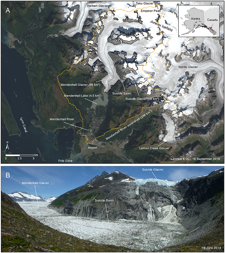
Figure 1. (A) Landsat Operational Land Imager (OLI) true color composite from 16 September 2018, showing the Mendenhall River watershed and surrounding areas. Key features and places are annotated. (B) Photo taken from the southeast corner of Suicide Basin toward the basin entrance and Mendenhall Glacier. Note the floating ice tongue and the elevation drop from the main glacier into the basin. On 19 June 2018 (date of photo), the water level in the basin was ~24 m below peak level.

FIGURE 2

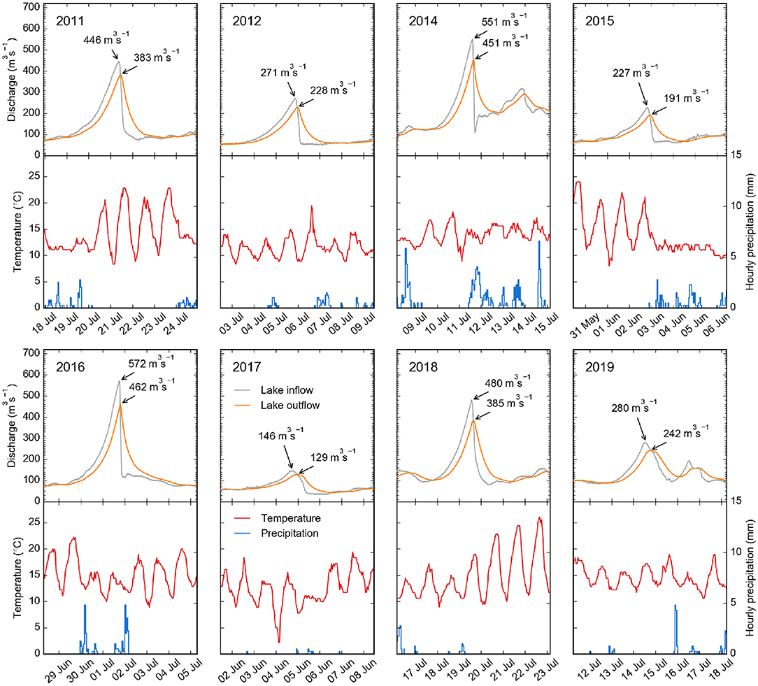
Figure 2. Main GLOF events observed between 2011 and 2019 at Mendenhall Lake and Mendenhall River. There is no panel for the 2013 event, which featured early and slow lake drainage at Suicide Basin, with no distinguishable reaction at Mendenhall Lake. (Top) panels show Mendenhall Lake inflow (gray lines) and outflow (orange lines). (Bottom) panels show the corresponding meteorological variables measured at Juneau Airport. The Mendenhall Lake outflow, which corresponds to the Mendenhall River discharge, is derived from the Mendenhall Lake level via rating curve for USGS station 15052500 (U.S. Geological Survey, 2019). The Mendenhall Lake inflow Q_in is calculated in a mass conserving fashion by differencing lake outflow Q_out and changes in lake storage, Q_in = Q_out + A · dh/dt, where A is the lake area (a function of the water level) and dh/dt the rate of the lake level change (Bartholomaus et al., 2015). Unlike previous events, the 2019 event caused two GLOF-related discharge peaks (on 14 and 16 July).

The current situation warrants comprehensive monitoring measures at Suicide Basin, which we present in this study. To contextualize the monitoring, we quantify the glacier change that has taken place at Suicide Basin since 2006, using remote sensing and in-situ data. We deepen the analysis for the years 2018 and 2019, during which we collected most of our data. Specifically, we assess surface mass balance, ice-flow dynamics, and lake evolution on sub-seasonal to multi-annual time scales, and discuss their impact on the basin's storage capacity. UAVs proved particularly useful for our work, hence, we emphasize their use in this paper.

2. Study Site

Mendenhall Glacier is a temperate maritime glacier that flows from the southwest side of the Juneau Icefield (Figure 1A). As of 2019, the glacier is 24.6 km long, covers 98 km², and spans an elevation range from 20 to 2,000 m a.s.l. (updated from Kienholz et al., 2015). Discharge from the glacier is released into proglacial Mendenhall Lake and subsequently flows into Mendenhall River, which meanders through residential areas toward Lynn Canal (Figure 1A). The Mendenhall River watershed covers 284 km², of which 120 km² (42%) are glacierized.

The glacier has been thinning and receding since the end of the Little Ice Age in the late eighteenth century (Motyka et al., 2002; Molnia, 2007). Retreat into an overdeepened basin resulted in the formation of Mendenhall Lake in the 1930s. Subsequent calving activity accelerated the glacier's recession, resulting in ~3 km of retreat during the twentieth century (Motyka et al., 2002; Boyce et al., 2007). Over the last two decades the glacier receded more than a kilometer, thinned by up to 150 m in its lower reaches, and had a resulting area-averaged mass balance of ~–0.7 m water equivalent (w.e.) a^–1 (Berthier et al., 2018). Modeling studies predict continued retreat during the twenty-first century (Ziemen et al., 2016).

Mendenhall Glacier's outburst floods originate from Suicide Basin, an ~0.7 km² partly glacierized basin located ~3 km upglacier from the terminus (Figure 1). Historically, ice flowed from Suicide Glacier into Mendenhall Glacier via Suicide Basin, whose ice surface elevation exceeded that of Mendenhall Glacier (Figure 3A). As a result of declining ice inflow from retreating Suicide Glacier, an ice depression started forming in the basin in the 1990s. Pooling water appeared in aerial images in the mid-2000s; however, no outburst floods were observed, which is characteristic for basins at the beginning of their jökulhlaup cycle (Clague and Evans, 1994; Geertsema and Clague, 2005). Suicide Glacier detached from Mendenhall Glacier entirely in 2006 (Figure 3B). Today, ice flows from Mendenhall Glacier into the basin and forms a temporarily sealed ice dam (Figures 1B, 3C). The water that fills the basin is stored beneath fractured remnant ice and also pools along the edges of the basin at high water levels. The thickness of the remnant ice in the basin was unknown prior to this study. Ice thickness measurements made outside of the basin suggest that the trunk glacier exceeds 500 m in thickness (Motyka et al., 2002).

FIGURE 3

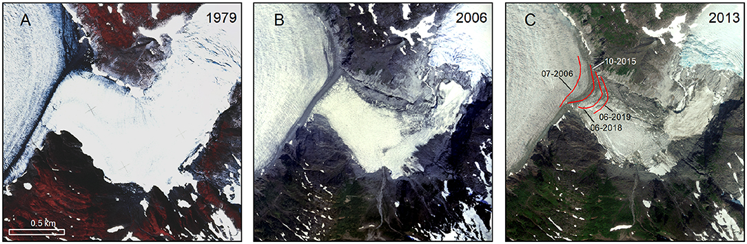
Figure 3. Orthophotos from (A) 11 August 1979, (B) 3 July 2006, and (C) 28 July 2013, showing the rapid decay of Suicide Basin's ice cover. The red lines in (C) trace the position of the former middle moraine from 2006 to 2019, revealing several hundred meters of ice motion into the basin. The WorldView-2 image shown in (C) was processed by the Polar Geospatial Center (www.pgc.umn.edu, © 2013, DigitalGlobe, Inc.).

3. Data

The University of Alaska Southeast (UAS) and the U.S. Geological Survey (USGS) have been monitoring Suicide Basin since 2012, in collaboration with Alaska's Division of Geological and Geophysical Surveys (DGGS), the National Weather Service (NWS) Juneau Forecast Office, the NWS Alaska-Pacific River Forecast Center, and the City and Borough of Juneau. The core monitoring setup comprises a seasonally deployed water level gauge, and since 2016, a telemetry-enabled time-lapse camera. Additional instruments have been deployed during some summers. The data that we collected are described in the following sections.

3.1. Water Level

Water level gauges have been deployed in the basin annually since 2012, however, the lake level only reached the gauges in 2012, 2014, 2016, 2018, and 2019. In 2018 and 2019, we installed two redundant Onset U20 loggers low in the basin (403 m above the WGS84 ellipsoid, henceforth m), with the goal of capturing most of the lake filling and drainage. During installation, we surveyed the logger location with a dual-frequency GPS (Trimble NetRS); GPS surveys of the water surface during subsequent site visits allowed for verification of the logger-derived water levels. In both years, thick ice debris deposited at the instrument site during lake drainage prevented instrument access for several weeks, but did not damage the loggers installed beneath a small overhang in the rock face. After recovery, we compensated the U20 data for variations in air pressure, using data from nearby Juneau Airport.

Prior to 2018, gauges were installed higher in the basin, and at different locations due to the evolving ice coverage. In 2016, water levels were surveyed with GPS and theodolite, which allowed for a direct adjustment of relative water-level elevations to the WGS84 ellipsoid, similar to 2018. In 2012 and 2014, gauge locations and water levels remained unsurveyed. We thus compared field photos from those years to a UAV-derived orthophoto from 2018 (section 4.1). Common features in the photos allowed us to trace the water level in the orthophoto and sample the corresponding elevations from the UAV-derived DEM (uncertainty within ~0.2 m).

3.2. Ice Elevation and Motion

3.2.1. GPS

In 2018, an on-ice GPS (Trimble NetRS) was deployed at the approximate center of the basin in the N-S direction and ~200 m from the basin entrance in the E-W direction (Figure 4). Due to problems with the power supply, the GPS only operated for a few weeks, missing lake drainage. The GPS recorded signals at 15 s intervals, which we postprocessed to spatial positions with cm accuracy, using the Precise Point Positioning service provided by Natural Resources Canada (https://webapp.geod.nrcan.gc.ca/geod/tools-outils/ppp.php). Given the unstable conditions on the floating ice tongue, we refrained from deploying an on-ice GPS in 2019.

FIGURE 4

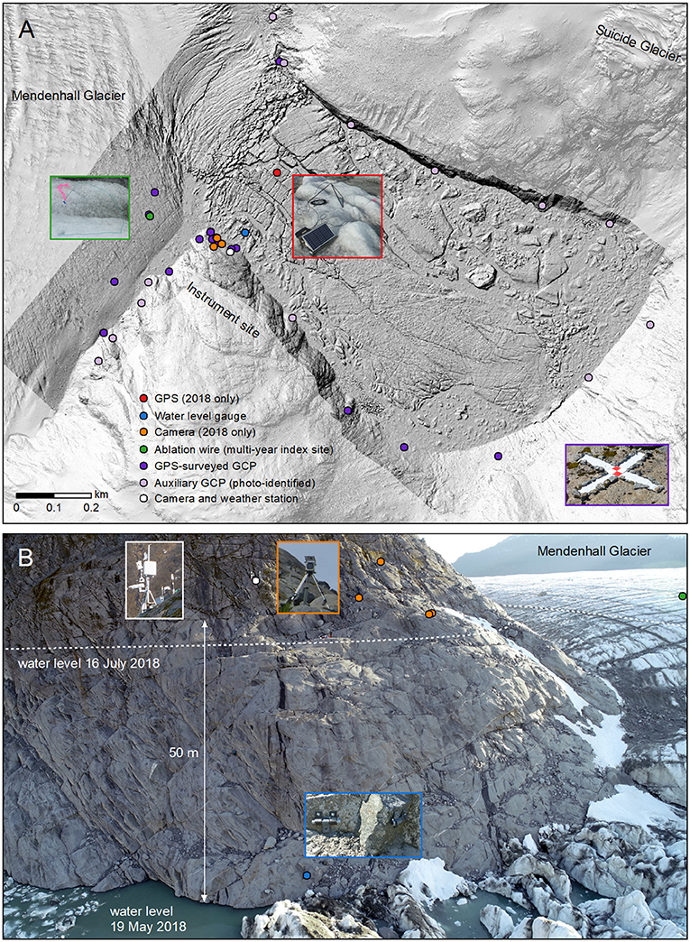
Figure 4. (A) Overview map of Suicide Basin, featuring location of deployed instruments as color-coded points. Color-coded photos show the instruments used. The background map consists of a shaded relief DEM based on UAV imagery from 17 July 2018 (~24 h after peak level). Outside the domain of the UAV DEM, laser data from 29 April 2018 completes the shaded relief DEM. (B) Aerial photo of the instrument site at the basin entrance. The photo was captured on 19 May 2018. Peak water level from 16 July 2018 is annotated for reference, as are the locations of key instruments from (A).

3.2.2. Time-Lapse Photos

From 2016 to 2019, a Remote Viewer system from Nupoint (http://www.nupointsystems.com/remote-viewer/) was used to image the central and back portion of Suicide Basin. The camera was mounted to a fixed pole located at the basin entrance at an elevation of 460 m (Figure 4). Photos were taken at daily to subdaily intervals and available via satellite link. The camera was removed prior to the winter season (in September or October) and remounted the following spring (in April or May). To achieve full coverage of Suicide Basin during the 2018 season, we also deployed four Harbortronics time-lapse systems (www.harbortronics.com/Products/TimeLapsePackage). These systems, built with Canon Rebel T5 cameras, were set up in the southwest corner of the basin (Figure 4) and provided photos every hour.

3.2.3. UAV-Borne Aerial Images

During the 2018 and 2019 seasons, we used a quadcopter UAV (DJI Phantom 4 Pro) to collect vertical aerial images across the basin, with the goal of building DEMs and orthomosaics via structure-from-motion (SFM) photogrammetry (Westoby et al., 2012). We conducted 9 UAV campaigns in 2018 and 8 campaigns in 2019. The UAV flew 120 m above the take-off point (located in the southwest corner of the basin) at a speed of 5.9 m s^–1 and acquired photos every 2 s, resulting in images with a ground resolution of ~3.3 cm pixel^–1 and ~90% front overlap. Flight line spacing was ~50 m, resulting in ~70% image sidelap. We collected ~1,700 images per campaign, covering the basin and a swath along the basin entrance (Figure 4). Camera settings were chosen semi-automatically (shutter-priority mode) or manually to guarantee sharp and well exposed images (O'Connor et al., 2017). Our ground control points (GCPs) consisted of 30 × 30 cm tiles placed in accessible areas around the basin (Figure 4). In inaccessible areas, we identified auxiliary GCPs in orthophotos and DEMs generated with a DJI Phantom 4 RTK UAV deployed in August 2019. The survey-grade Phantom 4 RTK UAV can achieve centimeter accuracy without the well-distributed GCPs needed for the Phantom 4 Pro UAV. This improved accuracy is owed to an onboard multi-band GNSS linked to a base station as well as accurate synchronization of GNSS and camera shutter timing.

3.2.4. Airborne Lidar

To collect additional topographic reference data across Suicide Basin and surrounding terrain, we conducted an airborne Lidar survey on 29 April 2018. The survey relied on a Riegl VUX-1-LR laser scanner (200 kHz pulse repetition rate, 49 Hz scan rate) with a Phoenix LiDAR Systems control unit and a LN200C IMU (200 Hz logging rate). A Novatel dual-band GNSS recorded aircraft coordinates at a 1 Hz rate. Flying ~200 m above the terrain at a ~125 km h^–1 ground speed, the plane covered multiple lines across the basin and surrounding terrain, which ensured 50% data overlap, minimal laser shadowing, and sufficient point density. We used Terrasolid and ArcMap to postprocess the Lidar data into a 0.1 m bare-earth DEM.

3.2.5. Legacy Aerial Photos and DEMs

To constrain basin evolution on longer timescales, we processed conventional film-based aerial photos from 3 July 2006 into DEMs and orthophotos (section 4.1). The photos were collected for the USGS using a Zeiss RMK TOP 15 aerial camera (153.22 mm focal length) flown at an elevation of ~3,500 m. We also processed aerial images from 1979 and 2015, but used only the resulting orthoimages to track moraine motion. The 2015 images were taken by DGGS during a helicopter-borne survey of Suicide Basin. The 1979 images were taken as part of the state-wide Alaska High-Altitude Aerial Photography (AHAP) campaign (Brooks, 1988; Kienholz et al., 2016).

We also analyzed DEMs from WorldView (WV) satellites, available to us for the years 2013 and 2016 via PGC's ArcticDEM portal (https://www.pgc.umn.edu/data/arcticdem; Porter et al., 2018). We used the DEMs from 28 July 2013 and 21 August 2016 specifically to determine elevation changes across the study area.

3.3. Surface Mass Balance and Meteorological Data

To measure in-situ surface mass balance, we installed weighted wires in the ice at the basin entrance (mass-balance index site at ~455 m, Figure 4). We re-measured the wire length during our site visits, collecting a total of 15 point-scale ablation measurements between 2018 and 2019. In 2016, a wire was installed at the same location and measured in spring and fall.

To measure in-situ air temperatures during the 2018 and 2019 summer seasons, we deployed a HOBO U23 Pro v2 sensor off-ice at the basin entrance (Figure 4). We mounted the sensor to a 2 m vertical pole at 460 m, roughly at the same elevation as and ~250 m away from the mass-balance index site. In 2019, we also deployed a tipping-bucket rain gauge (HOBO RG3-M) at the same pole. The 2018 and 2019 measurements complement precipitation and temperature records from 2016 conducted at the same location. We used the meteorological data to calibrate a classical temperature-index melt model (section 4.4). Since this model type performs better when forced by off-ice temperatures (Lang and Braun, 1990), we did not measure on-ice temperatures at the mass balance index site.

4. Methods

4.1. Derivation of DEMs and Orthophotos

We used Agisoft Metashape to process the UAV-based aerial photos. This software package provides a complete SFM workflow automatable via the Python programming language. We followed the standard workflow, comprising photo alignment, dense point cloud derivation, and DEM and orthophoto construction (e.g., Immerzeel et al., 2014; Gindraux et al., 2017). To process the Phantom 4 Pro images, we used 12 artificially marked GCPs and up to 14 auxiliary GCPs. To process the Phantom 4 RTK images, we relied on only one GCP and used the remaining survey points as check points. An average root mean square error (RMSE) of ~0.05 m at the check points indicated high quality of the RTK DEM across the basin. During the August 2019 campaign, we deployed the two UAVs in parallel to assess the vertical accuracy of the Phantom 4 Pro DEM, using the RTK DEM as a reference. Within the elevation band covered by the GCPs (~440–460 m), the mean elevation difference (Δz) between the DEMs was negligible (0.007 m with a standard deviation of 0.4 m). Outside the 440–460 m elevation band, we found a linear elevation-dependent bias in the Phantom 4 Pro DEM, reaching ~0.4 m at the 380–390 m elevation band, due to the lack of vertical control. We note that most of our DEM-derived measurements were taken above 380 m, where we expect smaller biases. Several hand-digitized waterlines, which we sampled along the Phantom 4 Pro DEMs, lay within ~0.3 m of the corresponding gauge reading, corroborating decimeter accuracy for the Phantom 4 Pro DEMs. In light of the large signals observed in the basin (several tens of meters), this decimeter accuracy introduces small relative uncertainties in the final results.

We also used Metashape to derive DEMs and orthoimages from the 2006 aerial images. For GCPs, we used terrain features located around the basin, identifiable both in the 2018 Lidar DEM and the 2006 aerial images. In the case of the 2006 aerial photos, the alignment resulted in an average RMSE of 0.50 m at the 9 GCPs. Differencing the 2006 DEM and the 2018 Lidar DEM across 0.35 km² of stable terrain yielded a mean elevation difference of 0.18 m and a standard deviation of 1.94 m. Some higher-order undulations emerged in the 2006 DEM and propagated into the final elevation difference maps, however, given the large elevation changes across the glacierized areas, the corresponding relative errors remained small (we compared the 2006 DEM to the 2018 Lidar DEM to determine long-term elevation changes).

The WorldView data obtained from Porter et al. (2018) were already processed into DEMs with 2 m spatial resolution. Prior to the DEM differencing, we coregistered the two DEMs from 28 July 2013 and 21 August 2016, using the approach of Nuth and Kääb (2011) and 0.65 km² of stable terrain around the basin as a local reference. After coregistration, the DEMs had a mean elevation difference of 0.08 m, with a standard deviation of 0.71 m.

4.2. Derivation of Ice Volume, Ice Thickness, and Bedrock Elevation

To estimate ice thickness and ice volume in the basin, we exploited the fact that ~10% of the ice volume extends above the waterline in the case of free-floating ice (hydrostatic equilibrium assumption, Sturm and Benson, 1985; Cuffey and Paterson, 2010). We measured ice freeboard by subtracting DEMs taken close to peak water level from horizontal planes representing the water surface. Multiplying with factor 10 and integrating across a manually digitized basin ice mask provided the total ice volume. In our calculations, we ignored density anomalies caused by the unknown debris concentration in the ice (Tweed, 2000).

By subtracting the derived ice thickness from a DEM taken after drainage (grounded stage), we estimated bedrock elevations, similar to Sturm and Benson (1985). We applied the approach only to small tabular icebergs that had maintained their original orientation (i.e., did not capsize), appeared to be free-floating pre-drainage, and grounded post-drainage. These criteria were fulfilled at the basin entrance in 2018. The floating ice tongue (fractured, but not fully broken up yet) was deemed unsuitable for local ice-thickness measurements: due to flexure, some of the ice was not in hydrostatic equilibrium, which biased local freeboard measurements.

4.3. Derivation of Ice Velocity Fields

To quantify ice motion, we tracked features on sequential shaded relief DEMs derived from the UAVs. We used Python's openPIV package (https://pypi.org/project/OpenPIV/, Taylor et al., 2010), which calculates normalized cross correlation between image patches to quantify their similarity. Tests with power-of-two sized correlation windows (which allow for efficient Fast Fourier Transforms) suggested an ideal correlation window size of 512 × 512 pixels (51.2 × 51.2 m), which we also chose for the search window size. During postprocessing, we assessed the velocity fields from openPIV visually and removed erroneous velocities.

We applied the same tracking approach (correlation window size of 64 × 64 pixels) to the oblique photos from the Nupoint time-lapse cameras, using pairs of photos taken 24 h apart (at 6:00 a.m. to avoid effects from sun shadows). We used these tracking results to determine the vertical motion of the ice tongue. These data proved particularly useful to track ice and water level changes beyond the range of the water level gauge.

4.4. Surface Mass-Balance Modeling

We used the 2018 and 2019 ice melt measurements (section 3.3) to calibrate a classical temperature-index melt model (also called degree-day model, e.g., Braithwaite, 1995; Ohmura, 2001; Hock, 2005) for the mass-balance index site at the basin entrance. Melt, M (mm w.e. h^–1), was derived from hourly average air temperature, T (°C), by

$\begin{array}{ll}M=\{\begin{array}{cc}{f}_{snow/ice}·T& \text{:}T>0\\ 0& \text{:}T<0\end{array},& (1)\end{array}$

where f_snow/ice are the melt factors of snow and ice (mm w.e. h⁻¹ °C⁻¹). We coupled the melt model to an accumulation model that kept track of the solid part of the precipitation. A linear function between 0.5 and 2.0°C allowed for a smooth transition between solid and liquid precipitation. We employed ice and snow melt factors of 0.237 mm w.e. h⁻¹ °C⁻¹ and 0.190 mm w.e. h⁻¹ °C⁻¹, respectively; this parameter combination yielded an RMSE of 0.15 m w.e. using 15 ice-melt measurements collected at the index site between 2018 and 2019. Validation with the 2016 season-long melt measurement (5.5 m w.e.) yielded a difference of 0.27 m w.e. (modeled melt more pronounced).

To run the model over the 2006–2019 period, we leveraged the air temperature and precipitation records from Juneau Airport, located 12 km from Suicide Basin near sea level (Figure 1). Temperature and precipitation showed distinct differences between basin and airport, due to the elevation difference (460 vs. 6 m), surrounding topography (basin with steep walls vs. open terrain), and land cover (snow and ice vs. wetland and ocean). High temperatures at the airport coincided with large temperature differences between the sites. Converted to lapse rates, the differences reached nearly –0.03°C m^–1 when measuring 25°C at the airport. In contrast, low summer temperatures (e.g., 5°C at the airport) coincided with smaller temperature differences (approximately –0.006 °C m^–1 converted to lapse rates). A linear regression (T_B = 0.468 + 0.457·T_A) captured these differences and was thus used to model the temperature at Suicide Basin (T_B) as a function of the Juneau Airport (T_A) temperature. To account for differences in precipitation, we compared the precipitation sums measured at Suicide Basin in 2016 and 2019 to the corresponding sums measured at the airport. The comparison indicated that precipitation in the basin is approximately 1.75 times greater than that at the airport. We used this factor to model the precipitation at the basin as a function of the airport precipitation.

5. Results

5.1. Glacier Change Since 2006

To contextualize our observations from 2018 and 2019, we assessed glacier thinning across the study domain for the 11.8 year period July 2006–April 2018, and the 3.1 year sub-period July 2013–August 2016. The choice of the two periods was partly dictated by the suitability of DEM pairs for comparison (e.g., two WorldView DEMs in the case of the 2013–2016 comparison). Our analysis focuses on the basin entrance; since this area hosts the ice dam, its evolution is of particular interest. Unlike ice in the basin, the ice at the basin entrance is grounded, so that elevation changes from DEM differencing translate directly into glacier thinning.

From July 2006 to April 2018, the basin entrance thinned by ~2.5 m a^–1 (Figure 5A). Thinning accelerated over recent years, as suggested by ~5 m a^–1 thinning rates over the sub-period July 2013–August 2016 (Figure 5B). The capture dates of the compared DEMs slightly exaggerate (2013–2016) or diminish (2006–2018) the actual thinning rates, but do not affect the overall acceleration trend, which agrees with observations on nearby Lemon Creek Glacier (O'Neel et al., 2019) and our mass-balance modeling (discussed below). In addition to varying temporally, thinning varied spatially across the basin entrance: it was less pronounced along the southern portion and more pronounced along the northern portion (transect A–B vs. B–C, Figure 5C). Since changes in surface mass balance are small across the basin entrance, differences in thinning must be controlled by ice-flow dynamics. More ice flow into the basin from the northern portion of the basin entrance likely caused the extra thinning in that area.

FIGURE 5

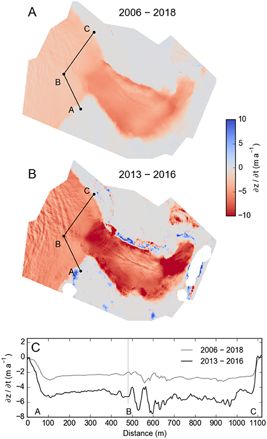
Figure 5. (A) Annual elevation changes (∂z/∂t) derived from differencing the Lidar-derived DEM from 29 April 2018 and the aerial photo-derived DEM from 3 July 2006. The black line shows the transect along which the elevation change is sampled in (C). (B) Annual elevation changes derived by differencing a WV3-derived DEM from 21 August 2016 and a WV2-derived DEM from 28 July 2013. Dark blue and red areas outside the glacier perimeter are due to DEM artifacts that occur mostly in steep terrain. White areas represent no data in the original DEMs. (C) Elevation changes sampled along the transect A–B–C across the basin entrance. Note the stronger thinning between B–C compared to A–B, caused by dynamic thinning due to ice flow into the basin.

Ice flow into the basin was estimated by tracking the location of the former middle moraine across several orthoimages (red lines in Figure 3C). The tracking yielded inflow rates of 15 m a^–1 (2006–2013), 26 m a^–1 (2013–2015), and 37 m a^–1 (2015–2018), thus confirming accelerated ice flow into the basin. GPS measurements in 1998 by Motyka et al. (2002) recorded ice motion into Suicide Basin of only 2 m a^–1. The observed ice-flow acceleration was driven by differential glacier thinning: more pronounced thinning inside the basin than outside (Figure 5) steepened the ice at the basin entrance, triggering additional inflow.

Surface mass-balance modeling complements the results from DEM differencing and moraine tracking. The mass-balance time series for 2006–2019 suggests annual surface mass balances between –5 and –8 m w.e. at the mass-balance index site, with more negative mass balances in recent years, as evidenced by the steepening of the time series (Figure 6A). These increasingly negative surface mass balances represent a key driver for the accelerating glacier thinning revealed by DEM differencing. Analysis of the meteorological data from Juneau Airport identifies rising summer temperatures as one of the main drivers for the negative mass-balance trend. After 2014, warm-humid or cold-dry winter seasons resulted in minimal winter mass gain, exacerbating the negative trend.

FIGURE 6

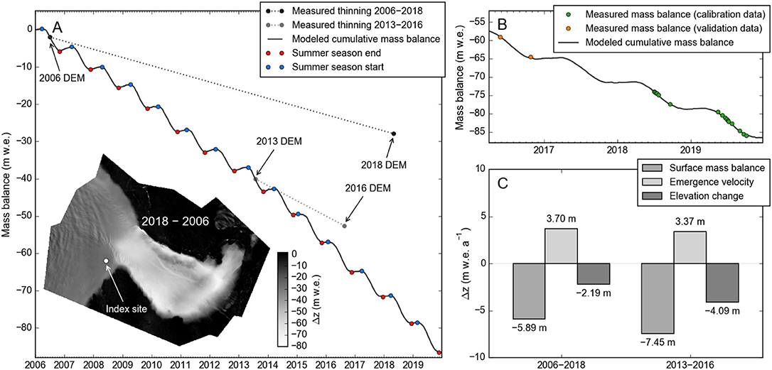
Figure 6. (A) Cumulative mass balance modeled for the index site outside Suicide Basin, period January 2006–December 2019. Colored dots denote annual maxima and minima in the mass balance series, which mark the start and end of the summer and winter seasons in the stratigraphic time system. The dotted lines show the glacier thinning in m w.e. obtained from differencing two DEM pairs (2006–2018 and 2013–2016, Figure 5). The inset map in (A) shows the ice thinning across the basin and the basin entrance derived from differencing the July 2006 and April 2018 DEMs. The map also shows the location of the mass balance index site. (B) The same cumulative mass balance series as in (A), but shown only for the 2016–2019 period, for which mass balance calibration and validation data was collected at the index site. (C) Annual surface mass balances, emergence velocities, and elevation changes for the two sub-periods with DEM availability. The emergence velocities are the difference between the modeled surface mass balance and the DEM-derived elevation changes in m w.e.

At the mass-balance index site, the DEM-derived glacier thinning was less negative than the modeled surface mass balance (Figure 6A). This difference is accounted for by emerging ice flow, which averaged 3.70 m w.e. a^–1 for the 2006–2018 period and 3.37 m w.e. a^–1 for the 2013–2016 period (Figure 6C). Inside the basin, observed thinning rates are much closer to the modeled surface mass balances (Figure 6A), suggesting reduced ice replenishment from ice flow. We note, however, that the glacier thinning inside the basin is difficult to quantify accurately, since ice may be floating in one or both DEMs compared.

The above observations quantified rapid ice decay inside Suicide Basin that exceeded loss of storage capacity due to ice dam thinning. Though ice flow into the basin accelerated rapidly, it failed to compensate for the large discrepancy in thinning rates between basin and basin entrance. This promoted the build-up of a large topographic depression and seasonal lake.

5.2. Seasonal Evolution of Suicide Basin's Lake and Ice Tongue

With Suicide Basin's ice dam thinning, peak lake levels in the basin decreased also, although premature lake drainages added variability to the overall trend. In 2012, the lake drained at 448 m, more than 15 m below the dam crest, which then reached an elevation of ~465 m at its lowest point. In 2014 and 2016, the lake expanded onto Mendenhall Glacier, but drained at 453 and 445 m, shortly before reaching the top of the ice dam. The premature drainage in 2017 occurred at 408 m, ~40 m below the ice dam crest. Only during the 2018 and 2019 seasons (described in detail next) did the water rise to the top of the ice dam and trigger overflow.

5.2.1. Year 2018

In 2018, the water level in Suicide Basin gradually rose from 388 m (29 April, first measurement) to 442.2 m (16 July, peak level), at an average rate of 0.7 m d^–1 (Figure 7A). During warm and wet periods (Figures 7C,D), the water level rose up to 1.6 m d^–1. An instant water-level drop of 0.75 m occurred during a large calving event on 25 June, which detached the basin's floating tongue from Mendenhall Glacier. During this unprecedented event, superbuoyant ice, forced under water next to the grounded glacier, broke off and rose to the surface, thereby increasing the basin's water storage capacity (Figure 8). Although the calving fractured a large section of the ice dam, it did not initiate drainage by damaging the seal. Early in July, the growing lake expanded onto the surface of Mendenhall Glacier and on 16 July the lake started overtopping the ice dam. The spillway followed the eastern glacier margin for several hundred meters and then re-entered the glacier via a moulin. Within ~24 h of overflow initiation, drainage transferred to a subglacial conduit and began to accelerate (day 1: ~1 m water level drop, day 2: 8 m, day 3: 35 m, Figure 7A). Drainage declined on the fourth day on 19 July, before the lake was empty. In total, lake level decreased by ~57 m to a surveyed elevation of 385.7 m one week after drainage initiation (Figure 9).

FIGURE 7

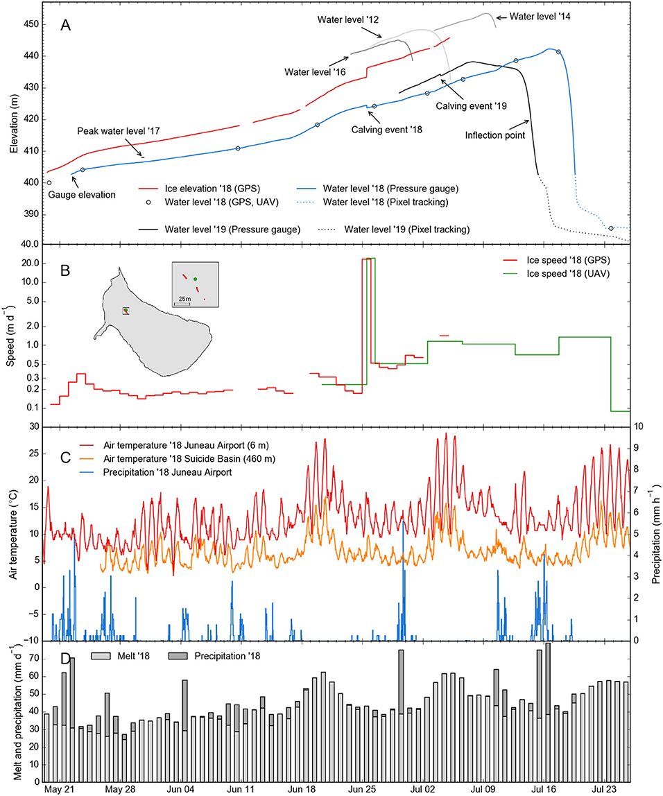
Figure 7. (A) Time series of water and ice elevation in Suicide Basin observed during the 2018 season (red and blue lines). Water levels for other seasons are plotted in gray tones, with rising limbs truncated to improve readability. In 2018, the on-ice GPS had intermittent data gaps early in the time series and failed to record the latter part of the time series because of a turned-over solar panel. (B) Horizontal speeds measured by the on-ice GPS (red curve, daily resolution) and sampled from the UAV-derived velocity fields (green curve, resolution dictated by the timing of the UAV campaigns). The inset map shows the GPS path (red trace) relative to the sampling location of the UAV-derived velocity fields (green point). During the calving event on 25 June, the floating tongue detached from the main glacier, with daily speeds increasing sharply to 25 m (note the logarithmic scale on the vertical axis). (C) Air temperature and hourly precipitation measured at Juneau Airport and in Suicide Basin. (D) Modeled daily melt and precipitation at the mass balance index site at the basin entrance at an elevation of ~455 m.

FIGURE 8

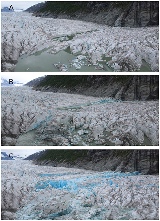
Figure 8. Time-lapse photos taken (A) before, (B) during, and (C) after Suicide Basin's floating ice tongue detached from the trunk glacier on 25 June 2018. Prior to the event, portions of the ice tongue were submerged entirely and thus superbuoyant. During the event, which occurred over a 15 min period, the ice rose by up to 10 m, and moved 25 m into the basin. Simultaneously, the water level in the basin dropped by 0.75 m.

FIGURE 9

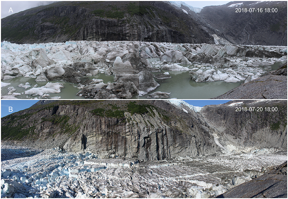
Figure 9. Panorama photos of Suicide Basin at (A) peak lake level and (B) after lake drainage, based on photos from two co-located Harbortronics time-lapse cameras. In 2018, the water level dropped more than 50 m during drainage. The ice tongue inside the basin stayed mostly afloat given the partial lake drainage.

Ice elevation generally followed lake level evolution, except for the calving event on 25 June, during which the ice surface rose while the water level dropped (Figure 7A). During lake drainage, ice located along the edge of the basin and at the basin entrance grounded, while ice in the central and back portion of the basin stayed afloat. During the monitored post-drainage period (20 July to 21 September) water and floating ice maintained a negative elevation trend, overlain by rapid fluctuations (up to ~10 m d^–1, Figure 10A). Two periods of water-level increase were sustained for more than a week, causing temporary water level increases on the order of 10–15 m. Two months after drainage on 21 September, we surveyed the water level at 374.9 m, 10.8 m below the post-drainage water level from 23 July. According to the time-lapse data, the lowest water level of the monitoring period was reached on 3 September at ~371 m (Figure 10A). Lake-level and mass-balance time series (Figure 10B) show matching seasonal trends, however, we found no clear correlation among short-term (i.e., daily or weekly) fluctuations. This may be related to the fact that the modeled mass balances represent point balances rather than watershed-wide balances (which we expect to be a better surrogate quantity for water flow into the basin).

FIGURE 10

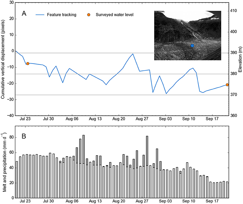
Figure 10. (A) Tracking-derived elevation changes of the floating Suicide Basin ice tongue following the main drainage event from 2018. The blue curve represents the cumulative vertical displacement sampled in the center of the basin (blue dot in the inset image). Two surveyed water levels (orange points) were used to tie pixel displacements into a metric vertical reference frame. Note this is an approximation only. (B) Daily melt (light gray bars) and precipitation (dark gray bars) modeled at the mass balance index site at the basin entrance, indicating decreasing water input into the glacier's hydrological system over the course of the late summer season.

The GPS- and feature tracking-derived velocities provide a detailed picture of the horizontal motion of the ice tongue during lake filling and drainage. Prior to the calving event, horizontal velocities at the basin entrance (GPS site) ranged between ~0.1 and 0.3 m d^–1 (Figures 7B, 11A). During the calving event, daily velocities increased by two orders of magnitude to 25–30 m d^–1 (Figures 7B, 11B), with most of the displacement accommodated over 15–20 min. The velocities decreased after the event, but remained higher than pre-calving at ~0.5–1 m d^–1 (Figures 7B, 11C–F). Lake drainage on 17 July created a concentric velocity field, with the ice tongue moving toward the basin center at up to 2 m d^–1 (Figure 11G). Over the 2 month post-drainage period, we observed continued ice flow toward the basin center at 0.1–0.15 m d^–1. At the basin entrance, ice inflow was on the order of 0.1–0.2 m d^–1 (Figure 11H), similar to the speeds observed at the beginning of the 2018 season. As hypothesized in section 5.1, ice flow into the basin occurs mostly across the northern portion of the basin entrance, explaining stronger dynamic thinning in that area.

FIGURE 11

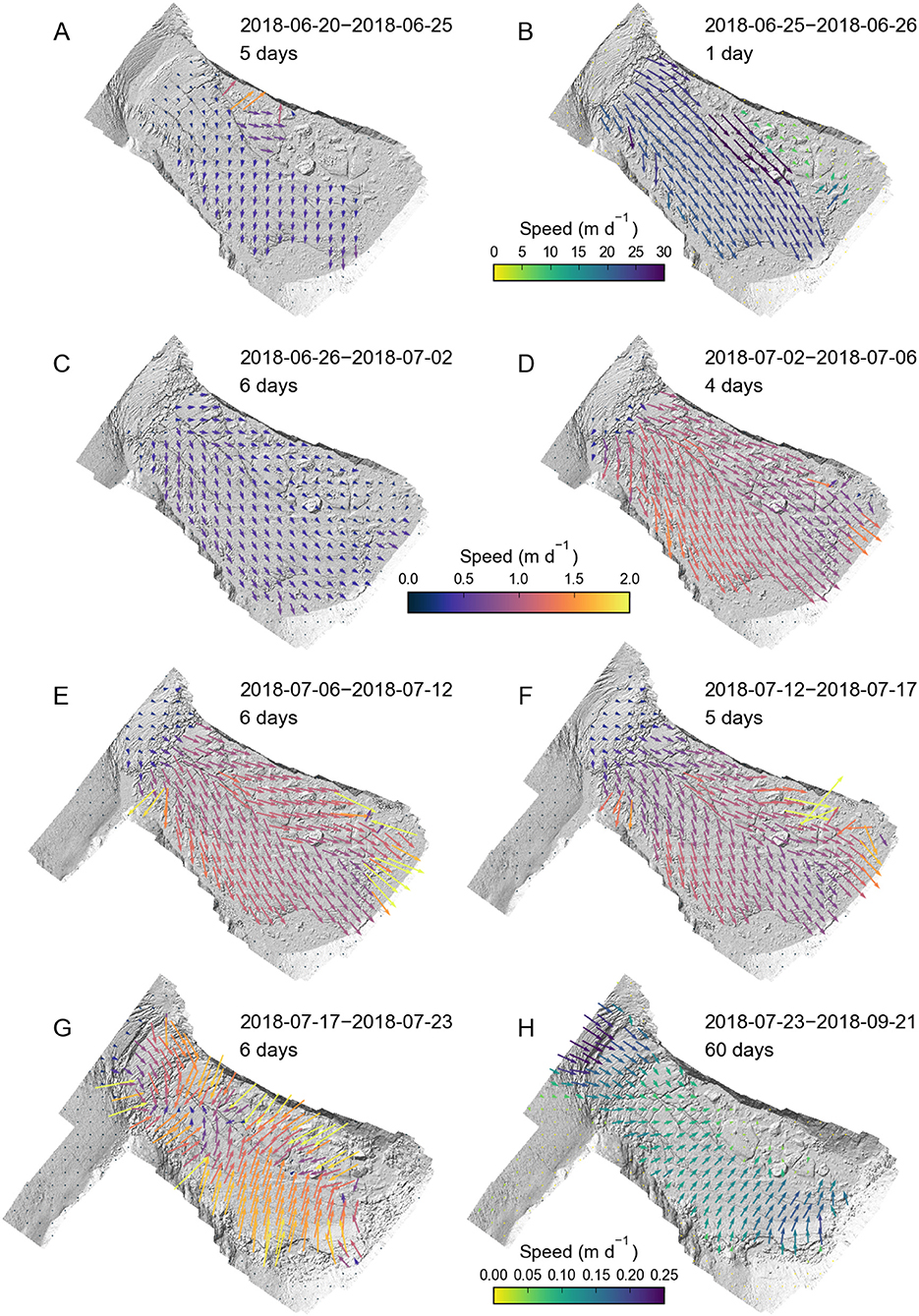
Figure 11. (A–H) Velocity time series derived from eight consecutive DEM pairs captured during summer 2018. Except for (B,H), the same vector scaling and colorbar (purple-red tones) applies across the panels. Panel (B), covering the calving event, and panel (H) covering the post-drainage period, capture periods with increased/reduced displacements, and thus feature their own vector scaling and colorbar in green-blue tones.

5.2.2. Year 2019

In 2019, the basin water level started lower than in 2018, but rose faster (1.0 vs. 0.7 m d^–1) due to unusually high summer temperatures. Similar to 2018, we observed a large calving event (on 4 July 2019), during which superbuoyant ice at the basin entrance detached from the ice dam (Figure 7A). The calving event caused a water level drop of 0.5 m, but as in 2018, did not initiate lake drainage. The lake overtopped the ice dam on 6 July at an elevation of ~437.5 m and reached its maximum level (438.2 m) on 7 July (Figure 7A). Overflow lasted approximately 6 days (as opposed to 1 day in 2018), with erosion at the crest of the ice dam exceeding 2 m (Figure 12). Steeper sections of the spillway farther downglacier were incised more than 4 m (Figure 13). The erosion rates remained approximately constant over the course of the overflow (Figure 7A). Thanks to the cold lake temperatures (~0.1°C, measured by our U20 sensors), accelerating spillway erosion, which is characteristic of unstable supraglacial drainage (Raymond and Nolan, 2000), did not occur.

FIGURE 12

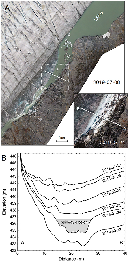
Figure 12. (A) Orthomosaic taken during the 2019 overflow event, showing Suicide Basin's lake extension and the spillway. The inset map shows the spillway after the overflow event. Transect A–B, along which topography is sampled in (B), extends across the dam's lowest portion. The 40 m transect covers an area of solid rock, the ice-cored moraine, the spillway, and relatively clean ice from Mendenhall Glacier. (B) Topography along transect A–B, sampled from six UAV-derived DEMs taken in 2018 and 2019. Spillway erosion during the 2018 overflow event was minimal; during the 2019 event, erosion reached ~2 m along the transect.

FIGURE 13

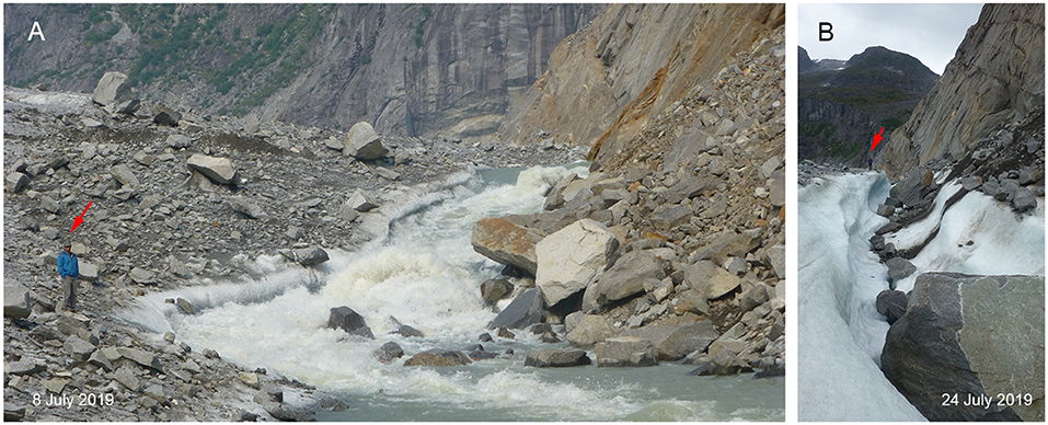
Figure 13. (A) Spillway during the second day of overflow on 8 July 2019. (B) Remnant spillway after 6 days of overflow. Note the person for scale (red arrow). Erosion reached up to 4 m in the imaged portion of the channel. The photo was taken on 24 July 2019, ~12 days after overflow ceased. Boulders and rocks partly filling in the channel originated from the ice-cored moraine.

Subglacial drainage started early on 12 July at a water level of ~436 m, and ended late on 16 July, taking about 5 days in total (1 day longer than in 2018). Drainage slowed down on 14 July at 420 m (see “inflection point” annotation in Figure 7A) and accelerated again at a level of ~400 m (on 16 July). This early and intermittent deceleration in lake drainage caused two flow peaks at Mendenhall River (U.S. Geological Survey, 2019), both of which were lower than the peaks of previous floods with similar lake volume (Figure 2). The post-drainage water level on 16 July was at ~386 m; on 24 July, we surveyed the water level at 383 m (Figure 7A). During the monitored post-drainage period (24 July to 18 September) the water level dropped relatively quickly and monotonically (as opposed to the fluctuations observed in 2018), reaching a surveyed water level of 341 m on 31 August and a time-lapse-derived level of 331 m on 18 September 2019. The September water level was ~50 m lower than the 2018 and 2019 post-GLOF levels, indicating that lake drainage during the 2018 and 2019 GLOF events was far from complete. Compared to the lowest water level measured in 2018 (~371 m), it was 40 m lower, suggesting that the post-GLOF water removal from the basin was more substantial in 2019 than in 2018.

5.3. GLOF and Post-GLOF Volume Changes 2018–2019

Differencing the 2018 pre-GLOF and post-GLOF DEMs (from 17 and 23 July, respectively) yielded a volume loss of 32 × 10⁶ m³ across the basin, which we attribute primarily to water removal during the GLOF event. For reference, this volume equates to more than 4 days of average July streamflow in the Mendenhall River. Our post-GLOF DEM was taken 4 days after termination of the main GLOF event; during these 4 days, the water level dropped an additional ~7 m, which accounted for ~3 × 10⁶ m³ of water. We thus estimate the water volume drained during the 2018 GLOF event to 29 × 10⁶ m³. Differencing the DEM from 23 July 2018 (post-GLOF) and 21 September 2018 (late season visit) provided an estimate of the post-GLOF elevation changes. Integrating these elevation changes across the basin yielded a volume loss of 7 × 10⁶ m³, attributable to additional water removal from the basin, ice melt, and some contribution from settling ice. Subtracting the contribution from surface melt (~2.2 m w.e. over the 60 day period) reduced this loss to 5 × 10⁶ m³, which we attribute primarily to post-GLOF water removal. This melt-corrected volume is equivalent to ~15–20% of the volume loss measured during the initial drainage.

Differencing the pre-GLOF and post-GLOF DEMs from 2019 (from 8 and 24 July) yielded a volume loss of 34 × 10⁶ m³ (Figures 14A–C,E–H). This volume estimate includes ~1.5 × 10⁶ m³ of water drained during the 6 day overflow period and ~1.5 × 10⁶ m³ of water drained after termination of the main GLOF event. Hence, we estimate the water volume drained during the 2019 GLOF event to 31 × 10⁶ m³. Differencing the DEM from 24 July 2019 (post-GLOF) and 31 August 2019 (last basin-wide DEM for 2019) yielded a volume loss of 15 × 10⁶ m³ (Figures 14D–H), of which we attribute 13 × 10⁶ m³ to post-GLOF water removal. This volume loss is equivalent to ~40% of the volume loss measured during the initial drainage. The post-GLOF volume loss in 2019 was more distinct than in 2018 (13 × 10⁶ m³ vs. 5 × 10⁶ m³), which confirms the more complete basin drainage described in section 5.2.2.

FIGURE 14

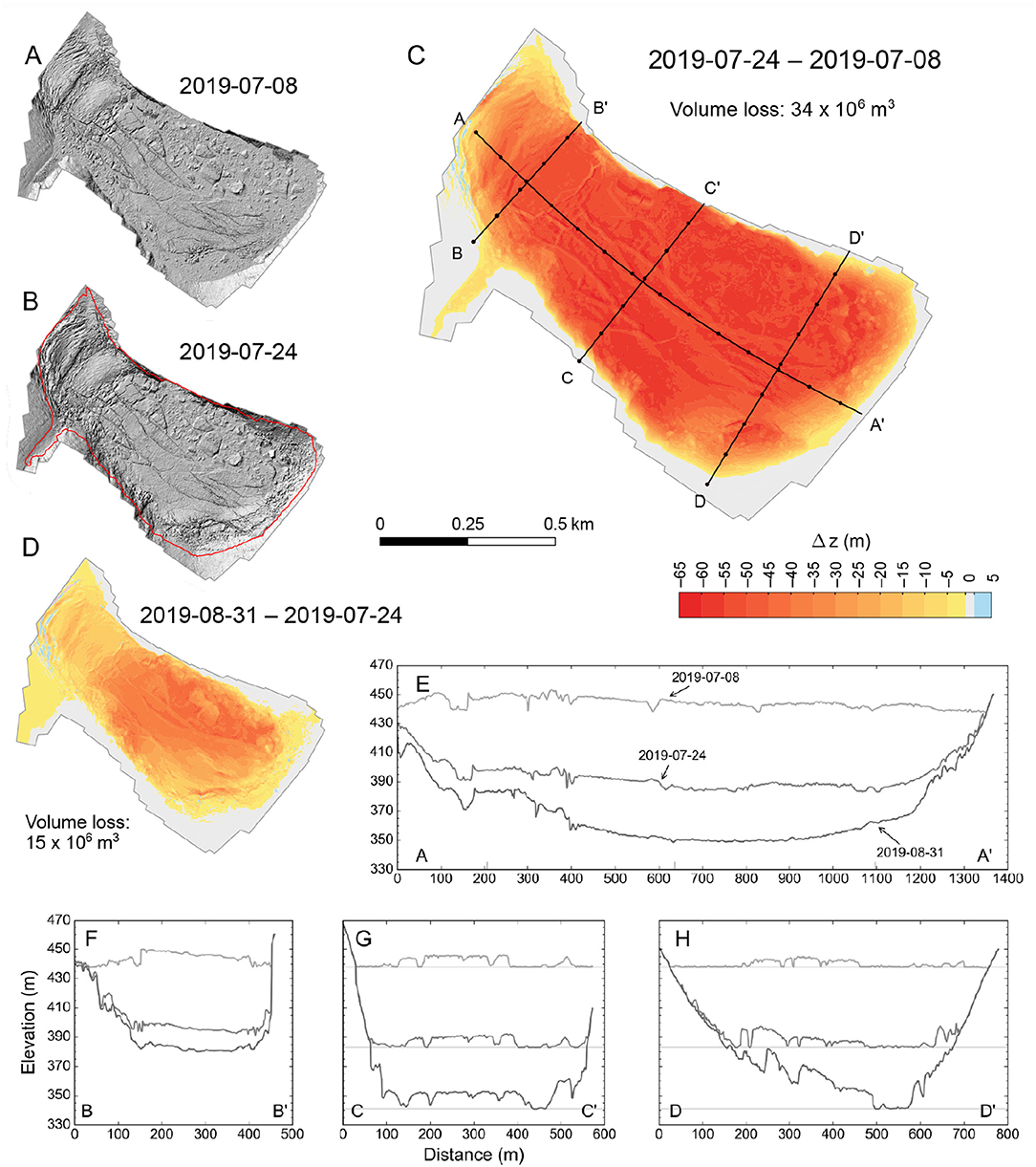
Figure 14. (A,B) Shaded relief DEMs from 8 and 24 July 2019, capturing the collapse of the floating ice tongue during lake drainage. (C) Elevation change map created by differencing the pre- and post-drainage DEMs from 8 and 24 July. The colormap features a 5 m color spacing, except for the ±1 m interval, which has its own gray tone. The annotated volume change (34 × 10⁶ m³) integrates the elevation changes across the perimeter of the maximum lake extent (0.76 km²), shown as red outline in (B). (D) Elevation change map covering the post-drainage period from 24 July to 31 August and utilizing the same colormap as (C). (E–H) Topography sampled along the longitudinal and transverse transects shown in (C). The water level for the three dates is shown with horizontal lines in (G,H). In (E), note the block of grounded ice at the basin entrance (between 0 and ~400 m), evidenced by reduced elevation changes.

The above DEM comparisons suggest that the water loss during the 2019 GLOF event exceeded the water loss during the 2018 event, although the ice dam had thinned by ~5 m over the same period. Several factors account for this observation: (1) The water level was lower in the 2019 post-GLOF DEM than in the 2018 post-GLOF DEM (383 vs. 386 m). (2) The basin expanded longitudinally during the 2019 calving event by ~100 m, which increased the basin's storage capacity (section 5.5). (3) Strong thinning of the ice tongue in the basin (section 5.4) helped increase the storage capacity. Regarding (3), we note that the thinning ice has limited influence on the GLOF volumes as long as lake drainage remains partial (i.e., as long as most of the ice stays afloat throughout drainage), which was the case both in 2018 and 2019.

5.4. Ice Volume Evolution in the Basin 2018–2019

Based on iceberg freeboard measurements conducted near peak level in 2018 (DEM from 17 July, water level 441.5 m a.s.l), we determined the volume of the floating ice in the lake (Figure 15). The freeboard height was 4.3 m on average, suggesting an average ice thickness of 43 m. This corresponds to a total ice volume of 29 × 10⁶ m³, which is equivalent to the water volume drained during the 2018 GLOF event. Within the basin proper (i.e., beyond the transect shown in Figure 15A), the freeboard height was 3.6 m on average, suggesting an average ice thickness of 36 m and a total ice volume of 22 × 10⁶ m³. Figure 15B shows ice thicknesses and glacier bed elevations along a transect at the basin entrance. Our measurements suggest maximum ice thicknesses of ~160 m (bed elevations down to ~230 m) and a total cross-sectional area of 35,000 m².

FIGURE 15

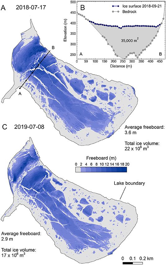
Figure 15. (A) Iceberg freeboard on 17 July 2018, calculated by subtracting the water level (441.5 m) from the DEM elevation. The annotated average freeboard elevations and ice volumes apply to the basin area beyond transect A–B. (B) Bedrock elevation across the basin entrance estimated by subtracting ice thickness estimates from 17 July 2018 (floating stage) from the ice surface measured on 21 September 2018 (grounded stage). Gray dots indicate location of the used ice thickness estimates. Gaps indicate areas with open water or overturned icebergs where freeboard measurements are not available/meaningful. (C) Same as (A), but for 8 July 2019 (water level 438.2 m).

We repeated ice freeboard measurements in 2019, using the DEM from 8 July (water level 438.2 m). The average freeboard reached 3.5 m across the entire lake (35 m total ice thickness), corresponding to a total ice volume of 25 × 10⁶ m³. Beyond the transect, the average freeboard was 2.9 m, equivalent to an ice thickness of 29 m and an ice volume of 17 × 10⁶ m³. Comparing the results from the two campaigns suggests that the average ice thickness in the basin (beyond the transect) decreased by ~6.3 m w.e. over the course of approximately one year (356 days). This loss corresponds to ~20% of the ice mass stored in the basin in 2018.

Considering an ice inflow of 0.1 m d^–1 across the 35,000 m² transect (plug flow assumption for simplicity) increases the ice melt estimate for the basin (6.3 m w.e. over 356 days) by ~2.0 m w.e. to ~8.3 m w.e. This exceeds the simultaneously recorded ice melt at the mass balance index site (7.6 m w.e. over 356 days) by 0.7 m w.e. The difference may be related to higher subaerial melt in the basin as well as subaqueous melt beneath the floating ice tongue. Enhanced subaerial melt is likely given the extra surface area exposed by the fractured ice inside the basin (especially after drainage with numerous stranded icebergs). Since the water temperatures in the lake remained close to freezing (~0.1 °C), we expect subaqueous melt to be small (which is characteristic for proglacial lakes; Truffer and Motyka, 2016).

5.5. Annual Elevation Changes 2018–2019

Our post-GLOF DEMs from 23 July 2018 and 24 July 2019 were taken almost exactly one year apart, which makes them ideal for mass balance applications and other benchmark measurements. DEM differencing across the mass balance index site yielded an elevation loss of 5.0 m a^–1, equivalent to 4.5 m w.e. a^–1 (Figure 16). For the same period, the wire-recorded mass loss was 7.8 m w.e. a^–1 and the residual ice emergence 3.3 m w.e. a^–1. The high melt and thinning rates were driven by the warm and dry weather and represent a continuation of the high melt and thinning rates measured in previous years (section 5.1, Figure 6). The 3.3 m w.e. a^–1 ice emergence is slightly lower (within uncertainties) than the emergence derived for the 2006–2018 period (3.7 m w.e. a^–1) and the 2013–2016 period (3.4 m w.e. a^–1). Decreasing ice emergence may reflect decelerating ice flow on main Mendenhall Glacier, driven by decades of negative glacier-wide mass balances (e.g., Heid and Kääb, 2012).

FIGURE 16

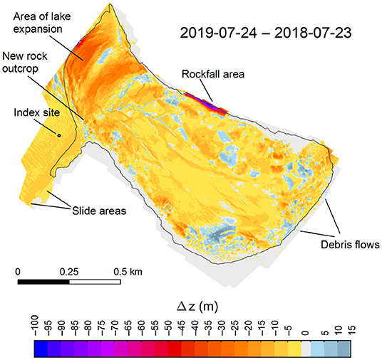
Figure 16. Elevation changes at Suicide Basin between 23 July 2018 and 24 July 2019. The differenced DEMs represent post-GLOF conditions, with similar water levels in the basin (386 m in 2018 and 383 m in 2019). The colormap features a 5 m color spacing, except for the ±1 m interval, which features a light gray tone. The black line delineates the maximum lake extent in 2019.

At the lowest point of the ice dam at the eastern glacier margin, glacier thinning was slightly higher than at the index site, reaching ~5.5 m a^–1 (Figure 16). Including the spillway erosion during the 2019 overflow event (~2 m, Figure 12B), the lowest point of the ice dam thinned by ~7.5 m between 2018 and 2019. In addition to the ice dam thinning, the DEM comparison revealed the impact of the 2019 calving event. During this event, the ice in the northern portion of the ice dam detached from the main glacier, pivoted, and moved into the basin, causing distinct thinning (20–40 m a^–1) at the basin entrance (Figure 16). The 2019 calving event occurred approximately 100 m further toward Mendenhall Glacier than the 2018 calving event, indicating longitudinal expansion of the basin.

In the northern portion of the ice dam outside the calved-off portion, thinning was on the order of 6 m a^–1, confirming generally higher (dynamic) thinning in that area compared to the southern portion of the ice dam. The northern portion of the ice dam appears to be much deeper, which likely explains higher rates of ice inflow and dynamic thinning in that area. On the south side, the transition into the basin occurs sharply (small, steep ice fall), with the upper portion of the ice underlain by a shallow bedrock rise. An isolated outcrop that emerged in the ice fall in spring 2019 (at ~ 413 m) is evidence of this bedrock rise.

As a side product, the DEM comparison revealed high geomorphological activity adjacent to the glacier (Figure 16). A large rockfall (~310,000 m³) originated in the rock face on the north side of the basin during the 2018–2019 winter season. Several smaller rockfalls took place in other areas of the rock face. We also found widespread erosion/deposition from debris flows in the back portion of Suicide Basin. Outside the basin next to Mendenhall Glacier, melting of the ice-cored side moraine caused several slides.

6. Discussion

6.1. Observed Patterns of Lake Filling and Drainage

Since Suicide Basin started releasing outburst floods in 2011, lake filling and drainage have followed an annual cycle, which is common for glacier-dammed marginal lakes (e.g., Clarke, 1982; Mathews and Clague, 1993; Walder et al., 2006; Ng and Liu, 2009). Lake filling occurred continuously for all events monitored, indicating separation of the basin from Mendenhall Glacier's hydrological system during the GLOF build-up, which matches observations at other locations (e.g., Clarke, 1982; Anderson et al., 2003b; Bartholomaus et al., 2008). Prior to 2018, the upward motion during lake filling was accommodated through flexure of the floating ice tongue, which resisted large bending stresses at the time. Rapid thinning and weakening of the ice tongue made the calving events of 2018 and 2019 possible. In both years, the floating tongue sheared off along steep fractures in the ice dam; as such, the calving events represent end members of the faulting mechanism discussed in Walder et al. (2006).

Subglacial drainage proceeded similarly for all GLOF events monitored at Suicide Basin: drainage started slowly, followed by a rapid increase over the course of a few days. This is in line with theory, which predicts conduit growth driven by dissipation of potential energy and sensible heat from the flowing water (e.g., Nye, 1976; Spring and Hutter, 1981; Fowler, 1999; Clarke, 2003). Regarding drainage initiation, we suspect a mechanism where the lake connects a subglacial conduit that has propagated up-glacier over the course of the melt season (e.g., Anderson et al., 2003a; Kessler and Anderson, 2004; Huss et al., 2007; Bartholomaus et al., 2011). Several premature drainages (e.g., in 2013, 2015, and 2017) and drainages after several days of overflow (2019) preclude ice dam flotation (e.g., Nye, 1976) as a trigger mechanism.

Time-lapse footage, available for the 2016–2019 events, suggests that drainage ceased well before Suicide Basin was empty. Such partial drainage is atypical for glacier-dammed marginal lakes (Post and Mayo, 1971; Mathews and Clague, 1993; Ng and Liu, 2009) and likely attributable to the extensive ice cover at Suicide Basin. At the basin entrance, we observed ice portions that sagged and grounded during the main GLOF events, analogous to the situation described in Anderson et al. (2003b). By obstructing the water's path to the outlet, sagging ice likely reduced the water flow through the outlet. This lowered the hydraulic head in the conduit and facilitated early conduit closure via ice creep (Fountain and Walder, 1998; Anderson et al., 2003b). Drainage re-acceleration, as observed in 2019, may have occurred once the outlet reopened due to melt or collapse of the ice obstacle. Alternatively, rather than outlet closure and reopening, transient changes in the hydraulic back-pressure from Mendenhall Glacier (Roberts et al., 2003; Bartholomaus et al., 2011) may have caused the observed intermittent outflow deceleration and re-acceleration.

The 2016–2019 time-lapse footage documented consistent post-GLOF behavior in that lake level trends were negative, with lowest lake levels toward the end of the monitoring period in September/October. Assuming that the lake level serves as a manometer for the glacier's hydrological system (Bartholomaus et al., 2011), this trend reflects declining water pressure therein, partly driven by decreasing surface melt (Fountain and Walder, 1998). Several cycles of partial lake filling and drainage were superimposed on the general trend during the 2016, 2017, and 2018 seasons, suggesting intermittently inverted hydraulic gradients (Roberts et al., 2003; Kingslake, 2015) or a partial sealing of the dam. In 2019, the lake level dropped largely monotonically, suggesting a less responsive connection to Mendenhall Glacier's hydrological system. Basin evolution was not monitored over the winter months, however, at the beginning of a new monitoring season (April, May), the water in the basin was typically tens of meters higher than in the previous fall. This suggests that the conduits that drained the basin resealed between late fall and late winter, re-initiating the next GLOF build-up.

6.2. Future Evolution of Suicide Basin

Suicide Basin has evolved rapidly over recent years and will continue to do so in the future. Some of the developments are predictable with high confidence, while others are more challenging to predict with the data available. It is certain that the floating ice tongue in the basin will disintegrate in the near future. Assuming a continuation of the current mass loss (7 m a^–1), disintegration is likely to occur within five years. Ice-dam thinning will also continue, likely at rates similar to those observed during the 2018–2019 season. Given declining ice emergence and continuing climate warming, ice-dam thinning may also accelerate. Projecting thinning rates of 5–6 m a^–1 into 2020, we expect the lowest point of the ice dam to lie at ~431 m in July 2020. Assuming that the lake will reach the top of the ice dam and drain to 386 m (partial drainage, similar to 2019), we project a GLOF volume of ~28 × 10⁶ m³, using the bathymetry surveyed in August 2019. This volume is smaller than the GLOF volume estimated in 2019 since longitudinal lake expansion at the basin entrance cannot compensate for the lower pre-drainage lake level expected for 2020 (431 vs. 436 m in 2019).

The above volume projection reflects just one scenario out of many possible combinations of pre- and post-drainage water levels. Considering Suicide Basin's drainage history and its most likely drainage mechanism (connection to an evolving subglacial conduit, rather than ice dam flotation, see previous section), premature lake drainage may occur instead of complete lake filling, which would reduce the projected GLOF volume. More complete lake drainage than observed in the past would increase the projected GLOF volume. Given the abundance of large fractured ice blocks at the basin entrance (which we suspect interrupt lake drainage by sagging, see previous section), more complete lake drainage appears unlikely within the next year or two. However, we hypothesize that this may change in the more distant future as ice cover in the basin continues to be lost. More complete lake drainage could slow or intermittently invert a trend toward smaller GLOF volumes, which we otherwise expect given the shrinking ice dam and limited potential for further longitudinal basin growth.

Our observations documented Suicide Basin's transition from an early stage in the jökulhlaup cycle (Clague and Evans, 1994) to today's advanced stage, a transition that matches the history of other basins in the region (Mathews and Clague, 1993; Geertsema and Clague, 2005; Neal, 2007; Capps et al., 2010). Given the current ice thickness at the basin entrance, the jökulhlaup cycle may continue for another decade or two, until Mendenhall Glacier has thinned too much to form a substantial ice dam.

7. Conclusions and Outlook

We presented a comprehensive set of remote sensing and in-situ data collected at glacier-dammed Suicide Basin between 2018 and 2019. Using UAVs extensively, we monitored lake build-up and drainage, and assessed our observations with auxiliary data collected since 2006. During the 2018 and 2019 events, ~30 × 10⁶ m³ of water drained from the basin, with the lake level falling more than 50 m over the course of a few days. Supraglacial outflow over the ice dam preceded subglacial lake drainage in both years, unlike in earlier events. Ice dam height (–5 m a^–1) and ice volume in the basin (–20% a^–1) declined rapidly over the course of the 2018–2019 season, largely given the unprecedentedly high surface melt (7.8 m w.e. from July 2018 to July 2019). While ice dam thinning reduces water storage capacity in the basin, declining ice volume and longitudinal growth of the basin counteract this trend. The potential for premature drainage onset (observed e.g., in 2015 and 2017), intermittent drainage decelerations (e.g., 2019), and early drainage termination (e.g., 2018) complicates predictions of GLOF timing and magnitude. While accurate GLOF predictions remain challenging, the data presented here provides the basis for realistic volume and drainage scenarios prior to future events.

We expect GLOFs from Suicide Basin to pose a threat over the next decade, hence we plan to continue the monitoring over the years to come. Monitoring of the basin remains crucial not only to detect current water level and drainage onset, but also to obtain updated lake bathymetries, which are needed for more accurate volume estimates. Starting in 2020 we will be using survey-grade UAVs routinely, which will reduce the amount of manual work during the photogrammetric post-processing, while also improving the accuracy of the resulting products. Tests during the 2019 season revealed the utility of modern fixed-wing Vertical Take-Off and Landing (VTOL) drones within our large and steep study domain. In 2019, we also started expanding the network of melt and temperature measurement sites up to Suicide Glacier (1,000 m a.s.l.). This will allow for a robust mass-balance model calibration across the entire Suicide Basin watershed (~17 km²) starting in 2020. Ideally, we will be able to model water input into Suicide Basin similar to Huss et al. (2007), which will provide a better understanding of lake filling and drainage, and potentially allow lake-level predictions based on weather forecast data.

Ultimately, a glacio-hydrological model (e.g., Ragettli et al., 2015; Beamer et al., 2016), running at hourly to sub-hourly resolution, should be established for the entire Mendenhall River watershed. The large size of the watershed (284 km²), variable types of surface cover, and complex temperature and precipitation gradients make this undertaking challenging at present. However, with the amount of available calibration data already unique by Alaska standards, only a few strategic measurements are required across the watershed to make this a reality. Among other applications, a calibrated glacio-hydrological model would allow for an assessment of baseflow during GLOF events all the way back to 2011. This would then enable accurate derivation of GLOF volumes from the Mendenhall River hydrographs. Together with our observations from the basin, these measurements could be used to attempt physical outburst flood modeling (e.g., Carrivick et al., 2017). This would provide additional insights into the underlying processes and likely improve our GLOF forecasting capabilities at Suicide Basin and elsewhere.

Data Availability Statement

Key data used for this study have been archived at the Arctic Data Center (https://doi.org/10.18739/A2GT5FG0B).

Author Contributions

CK designed the project, led data collection in 2018 and 2019, and wrote the paper. JP helped to design the project, collected field data from 2012 to 2019, and provided comments on the paper. EH, JA, GW, and AJ provided feedback on the project design, collected field data before and after 2018, and helped to write or commented on the paper. SH, DA-F, and KW assisted in the field and/or processed several datasets. CJ and JC helped with the project design, oversaw data collection, and commented on the paper.

Funding

This work was funded by the Alaska Climate Adaptation Science Center (AK CASC). UAVs and other surveying equipment were partly funded through the U.S. National Science Foundation (NSF) award EAR-1921598. EH and SH were partially supported by the NSF award OIA-1753748 and the State of Alaska. Streamflow monitoring of the Mendenhall River and real-time imagery of Suicide Basin were funded by the U.S. Geological Survey Groundwater and Streamflow Information Program. Any use of trade, firm, or product names is for descriptive purposes only and does not imply endorsement by the U.S. Government.

Conflict of Interest

The authors declare that the research was conducted in the absence of any commercial or financial relationships that could be construed as a potential conflict of interest.

Acknowledgments

We thank Chris Waythomas, Gwenn Flowers, and Mauro Werder for their comments that strengthened the initial version of this paper.

References

Anderson, S. P., Longacre, S. A., and Kraal, E. R. (2003a). Patterns of water chemistry and discharge in the glacier-fed Kennicott River, Alaska: evidence for subglacial water storage cycles. Chem. Geol. 202, 297–312. doi: 10.1016/j.chemgeo.2003.01.001

CrossRef Full Text | Google Scholar

Anderson, S. P., Walder, J. S., Anderson, R. S., Kraal, E. R., Cunico, M., Fountain, A. G., et al. (2003b). Integrated hydrologic and hydrochemical observations of Hidden Creek Lake jökulhlaups, Kennicott Glacier, Alaska. J. Geophys. Res. 108. doi: 10.1029/2002JF000004

CrossRef Full Text | Google Scholar

Bartholomaus, T. C., Amundson, J. M., Walter, J. I., O'Neel, S., West, M. E., and Larsen, C. F. (2015). Subglacial discharge at tidewater glaciers revealed by seismic tremor. Geophys. Res. Lett. 42, 33–37. doi: 10.1002/2015GL064590

PubMed Abstract | CrossRef Full Text | Google Scholar

Bartholomaus, T. C., Anderson, R. S., and Anderson, S. P. (2008). Response of glacier basal motion to transient water storage. Nat. Geosci. 1:33. doi: 10.1038/ngeo.2007.52

CrossRef Full Text | Google Scholar

Bartholomaus, T. C., Anderson, R. S., and Anderson, S. P. (2011). Growth and collapse of the distributed subglacial hydrologic system of Kennicott Glacier, Alaska, USA, and its effects on basal motion. J. Glaciol. 57, 985–1002. doi: 10.3189/002214311798843269

CrossRef Full Text | Google Scholar

Beamer, J., Hill, D., Arendt, A., and Liston, G. (2016). High-resolution modeling of coastal freshwater discharge and glacier mass balance in the Gulf of Alaska watershed. Water Resour. Res. 52, 3888–3909. doi: 10.1002/2015WR018457

CrossRef Full Text | Google Scholar

Berthier, E., Larsen, C., Durkin, W. J., Willis, M. J., and Pritchard, M. E. (2018). Brief communication: unabated wastage of the Juneau and Stikine icefields (southeast Alaska) in the early 21st century. Cryosphere 12, 1523–1530. doi: 10.5194/tc-12-1523-2018

CrossRef Full Text | Google Scholar

Boyce, E. S., Motyka, R. J., and Truffer, M. (2007). Flotation and retreat of a lake-calving terminus, Mendenhall Glacier, southeast Alaska, USA. J. Glaciol. 53, 211–224. doi: 10.3189/172756507782202928

CrossRef Full Text | Google Scholar

Braithwaite, R. J. (1995). Positive degree-day factors for ablation on the Greenland ice sheet studied by energy-balance modelling. J. Glaciol. 41, 153–160. doi: 10.1017/S0022143000017846

CrossRef Full Text | Google Scholar

Brooks, P. D. (1988). The Alaska High-Altitude Aerial Photography (AHAP) Program. Technical report, State of Alaska.

Capps, D., and Clague, J. J. (2014). Evolution of glacier-dammed lakes through space and time; Brady Glacier, Alaska, USA. Geomorphology 210, 59–70. doi: 10.1016/j.geomorph.2013.12.018

CrossRef Full Text | Google Scholar

Capps, D., Rabus, B., Clague, J. J., and Shugar, D. H. (2010). Identification and characterization of alpine subglacial lakes using interferometric synthetic aperture radar (InSAR): Brady Glacier, Alaska, USA. J. Glaciol. 56, 861–870. doi: 10.3189/002214310794457254

CrossRef Full Text | Google Scholar

Carrivick, J. L., Tweed, F. S., Ng, F., Quincey, D. J., Mallalieu, J., Ingeman-Nielsen, T., et al. (2017). Ice-dammed lake drainage evolution at Russell Glacier, West Greenland. Front. Earth Sci. 5:100. doi: 10.3389/feart.2017.00100

CrossRef Full Text | Google Scholar

Clague, J. J., and Evans, S. G. (1994). Formation and Failure of Natural Dams in the Canadian Cordillera, Vol. 464. Geological Survey of Canada. doi: 10.4095/194028

CrossRef Full Text

Clarke, G. K. (1982). Glacier outburst floods from Hazard Lake, Yukon Territory, and the problem of flood magnitude prediction. J. Glaciol. 28, 3–21. doi: 10.1017/S0022143000011746

CrossRef Full Text | Google Scholar

Clarke, G. K. (2003). Hydraulics of subglacial outburst floods: new insights from the Spring-Hutter formulation. J. Glaciol. 49, 299–313. doi: 10.3189/172756503781830728

CrossRef Full Text | Google Scholar

Cuffey, K. M., and Paterson, W. S. B. (2010). The Physics of Glaciers. Amsterdam: Academic Press.

Google Scholar

Curran, J. H., Barth, N. A., Veilleux, A. G., and Ourso, R. T. (2016). Estimating Flood Magnitude and Frequency at Gaged and Ungaged Sites on Streams in Alaska and Conterminous Basins in Canada, Based on Data Through Water Year 2012. Technical report, US Geological Survey. doi: 10.3133/sir20165024

CrossRef Full Text | Google Scholar

Fountain, A. G., and Walder, J. S. (1998). Water flow through temperate glaciers. Rev. Geophys. 36, 299–328. doi: 10.1029/97RG03579

PubMed Abstract | CrossRef Full Text | Google Scholar

Fowler, A. C. (1999). Breaking the seal at Grimsvötn, Iceland. J. Glaciol. 45, 506–516. doi: 10.3189/S0022143000001362

CrossRef Full Text | Google Scholar

Geertsema, M., and Clague, J. J. (2005). Jökulhlaups at Tulsequah Glacier, northwestern British Columbia, Canada. Holocene 15, 310–316. doi: 10.1191/0959683605hl812rr

CrossRef Full Text | Google Scholar

Gindraux, S., Boesch, R., and Farinotti, D. (2017). Accuracy assessment of digital surface models from unmanned aerial vehicles' imagery on glaciers. Remote Sens. 9:186. doi: 10.3390/rs9020186

CrossRef Full Text | Google Scholar

Haemmig, C., Huss, M., Keusen, H., Hess, J., Wegmüller, U., Ao, Z., and Kulubayi, W. (2014). Hazard assessment of glacial lake outburst floods from Kyagar glacier, Karakoram mountains, China. Ann. Glaciol. 55, 34–44. doi: 10.3189/2014AoG66A001

CrossRef Full Text | Google Scholar

Heid, T., and Kääb, A. (2012). Repeat optical satellite images reveal widespread and long term decrease in land-terminating glacier speeds. Cryosphere 6, 467–478. doi: 10.5194/tc-6-467-2012

CrossRef Full Text | Google Scholar

Hock, R. (2005). Glacier melt: a review of processes and their modelling. Prog. Phys. Geogr. 29, 362–391. doi: 10.1191/0309133305pp453ra

CrossRef Full Text | Google Scholar

Huss, M., Bauder, A., Werder, M., Funk, M., and Hock, R. (2007). Glacier-dammed lake outburst events of Gornersee, Switzerland. J. Glaciol. 53:181. doi: 10.3189/172756507782202784

CrossRef Full Text | Google Scholar

Immerzeel, W., Kraaijenbrink, P., Shea, J., Shrestha, A., Pellicciotti, F., Bierkens, M., et al. (2014). High-resolution monitoring of Himalayan glacier dynamics using unmanned aerial vehicles. Remote Sens. Environ. 150, 93–103. doi: 10.1016/j.rse.2014.04.025

CrossRef Full Text | Google Scholar

Kessler, M. A., and Anderson, R. S. (2004). Testing a numerical glacial hydrological model using spring speed-up events and outburst floods. Geophys. Res. Lett. 31, 1–5. doi: 10.1029/2004GL020622

CrossRef Full Text | Google Scholar

Kienholz, C., Herreid, S., Rich, J., Arendt, A., Hock, R., and Burgess, E. (2015). Derivation and analysis of a complete modern-date glacier inventory for Alaska and northwest Canada. J. Glaciol. 61, 403–420. doi: 10.3189/2015JoG14J230

CrossRef Full Text | Google Scholar

Kienholz, C., Hock, R., Truffer, M., Arendt, A. A., and Arko, S. (2016). Geodetic mass balance of surge-type Black Rapids Glacier, Alaska, 1980-2001-2010, including role of rockslide deposition and earthquake displacement. J. Geophys. Res. 121, 1–24. doi: 10.1002/2016JF003883

CrossRef Full Text | Google Scholar

Kingslake, J. (2015). Chaotic dynamics of a glaciohydraulic model. J. Glaciol. 61, 493–502. doi: 10.3189/2015JoG14J208

CrossRef Full Text | Google Scholar

Lang, H., and Braun, L. (1990). On the information content of air temperature in the context of snow melt estimation. IAHS Publ. 190, 347–354.

Google Scholar

Mathews, W. H., and Clague, J. J. (1993). The record of jökulhlaups from Summit Lake, northwestern British Columbia. Can. J. Earth Sci. 30, 499–508. doi: 10.1139/e93-039

CrossRef Full Text | Google Scholar

Molnia, B. F. (2007). Late nineteenth to early twenty-first century behavior of Alaskan glaciers as indicators of changing regional climate. Glob. Planet. Change 56, 23–56. doi: 10.1016/j.gloplacha.2006.07.011

CrossRef Full Text | Google Scholar

Motyka, R. J., O'Neel, S., Connor, C. L., and Echelmeyer, K. A. (2002). Twentieth century thinning of Mendenhall Glacier, Alaska, and its relationship to climate, lake calving, and glacier run-off. Glob. Planet. Change 35, 93–112. doi: 10.1016/S0921-8181(02)00138-8

CrossRef Full Text | Google Scholar

Neal, E. (2007). Hydrology and Glacier-Lake Outburst Floods (1987-2004) and Water Quality (1998-2003) of the Taku River near Juneau, Alaska. USGS Scientific Investigations Report 2007–5027. doi: 10.3133/sir20075027

CrossRef Full Text | Google Scholar

Ng, F., and Liu, S. (2009). Temporal dynamics of a jökulhlaup system. J. Glaciol. 55, 651–665. doi: 10.3189/002214309789470897

CrossRef Full Text | Google Scholar

Nuth, C., and Kääb, A. (2011). Co-registration and bias corrections of satellite elevation data sets for quantifying glacier thickness change. Cryosphere 5, 271–290. doi: 10.5194/tc-5-271-2011

CrossRef Full Text | Google Scholar

Nye, J. F. (1976). Water flow in glaciers: Jökulhlaups, tunnels, and veins. J. Glaciol. 17, 181–207. doi: 10.3189/S002214300001354X

CrossRef Full Text | Google Scholar

O'Connor, J., Smith, M. J., and James, M. R. (2017). Cameras and settings for aerial surveys in the geosciences: optimising image data. Prog. Phys. Geogr. 41, 325–344. doi: 10.1177/0309133317703092

CrossRef Full Text | Google Scholar

Ohmura, A. (2001). Physical basis for the temperature-based melt-index method. J. Appl. Meteorol. 40, 753–761. doi: 10.1175/1520-0450(2001)040<0753:PBFTTB>2.0.CO;2

CrossRef Full Text | Google Scholar

O'Neel, S., McNeil, C., Sass, L. C., Florentine, C., Baker, E. H., Peitzsch, E., et al. (2019). Reanalysis of the US Geological Survey Benchmark Glaciers: long-term insight into climate forcing of glacier mass balance. J. Glaciol. 65, 850–866. doi: 10.1017/jog.2019.66

CrossRef Full Text | Google Scholar

Porter, C., Morin, P., Howat, I., Noh, M.-J., Bates, B., Peterman, K., et al. (2018). ArcticDEM. St Paul, MN: Polar Geospatial Center.

Google Scholar

Post, A., and Mayo, L. R. (1971). Glacier Dammed Lakes and Outburst Floods in Alaska. Washington, DC: US Geological Survey.

Google Scholar

Ragettli, S., Pellicciotti, F., Immerzeel, W. W., Miles, E. S., Petersen, L., Heynen, M., et al. (2015). Unraveling the hydrology of a Himalayan catchment through integration of high resolution in situ data and remote sensing with an advanced simulation model. Adv. Water Resour. 78, 94–111. doi: 10.1016/j.advwatres.2015.01.013

CrossRef Full Text | Google Scholar

Raymond, C. F., and Nolan, M. (2000). Drainage of a glacial lake through an ice spillway. IAHS Publ. 264, 199–210.

Google Scholar

Roberts, M. J. (2005). Jökulhlaups: a reassessment of floodwater flow through glaciers. Rev. Geophys. 43, 1–21. doi: 10.1029/2003RG000147

CrossRef Full Text | Google Scholar

Roberts, M. J., Tweed, F. S., Russell, A. J., Knudsen, Ó., and Harris, T. D. (2003). Hydrologic and geomorphic effects of temporary ice-dammed lake formation during jökulhlaups. Earth Surf. Process. Landforms 28, 723–737. doi: 10.1002/esp.476

CrossRef Full Text | Google Scholar

Spring, U., and Hutter, K. (1981). Numerical studies of jökulhlaups. Cold Regions Sci. Technol. 4, 227–244.

Google Scholar

Sturm, M., and Benson, C. S. (1985). A history of jökulhlaups from Strandline Lake, Alaska, USA. J. Glaciol. 31, 272–280. doi: 10.1017/S0022143000006602

CrossRef Full Text | Google Scholar

Taylor, Z. J., Gurka, R., Kopp, G. A., and Liberzon, A. (2010). Long-duration time-resolved PIV to study unsteady aerodynamics. IEEE Trans. Instrum. Measure. 59, 3262–3269. doi: 10.1109/TIM.2010.2047149

PubMed Abstract | CrossRef Full Text | Google Scholar

Truffer, M., and Motyka, R. J. (2016). Where glaciers meet water: subaqueous melt and its relevance to glaciers in various settings. Rev. Geophys. 54, 220–239. doi: 10.1002/2015RG000494

CrossRef Full Text | Google Scholar

Tweed, F. S. (2000). Jökulhlaup initiation by ice-dam flotation: the significance of glacier debris content. Earth Surf. Process. Landforms 25, 105–108. doi: 10.1002/(SICI)1096-9837(200001)25:1<105::AID-ESP73>3.0.CO;2-B

CrossRef Full Text | Google Scholar

U.S. Geological Survey (2019). USGS Water Data for the Nation: U.S. Geological Survey National Water Information System Database. doi: 10.5066/F7P55KJN

CrossRef Full Text

Vincent, C., Auclair, S., and Le Meur, E. (2010). Outburst flood hazard for glacier-dammed Lac de Rochemelon, France. J. Glaciol. 56, 91–100. doi: 10.3189/002214310791190857

CrossRef Full Text | Google Scholar

Walder, J. S., Trabant, D. C., Cunico, M., Fountain, A. G., Anderson, S. P., Anderson, R. S., et al. (2006). Local response of a glacier to annual filling and drainage of an ice-marginal lake. J. Glaciol. 52, 440–450. doi: 10.3189/172756506781828610

CrossRef Full Text | Google Scholar

Werder, M., Bauder, A., Funk, M., and Keusen, H.-R. (2010). Hazard assessment investigations in connection with the formation of a lake on the tongue of Unterer Grindelwaldgletscher, Bernese Alps, Switzerland. Nat. Hazards Earth Syst. Sci. 10, 227–237. doi: 10.5194/nhess-10-227-2010

CrossRef Full Text | Google Scholar

Westoby, M. J., Brasington, J., Glasser, N. F., Hambrey, M. J., and Reynolds, J. M. (2012). Structure-from-motion photogrammetry: a low-cost, effective tool for geoscience applications. Geomorphology 179, 300–314. doi: 10.1016/j.geomorph.2012.08.021

CrossRef Full Text | Google Scholar

Wolfe, D. F. G., Kargel, J. S., and Leonard, G. J. (2014). “Chapter: Glacier-dammed ice-marginal lakes of Alaska,” in Global Land Ice Measurements from Space, ed J. S. Kargel (Berlin; Heidelberg: Springer), 263–295. doi: 10.1007/978-3-540-79818-7_12

CrossRef Full Text | Google Scholar

Ziemen, F., Hock, R., Aschwanden, A., Khroulev, C., Kienholz, C., Melkonian, A., et al. (2016). Modeling the evolution of the Juneau Icefield between 1971 and 2100 using the Parallel Ice Sheet Model (PISM). J. Glaciol. 62, 199–214. doi: 10.1017/jog.2016.13

CrossRef Full Text | Google Scholar