Mapping of High-Spatial-Resolution Three-Dimensional Electron Density by Combing of Full-Polarimetric SAR and IRI Model

Introduction

The ionosphere, extending from ~60 to 1,000 km above the earth's surface, is an important part of the solar–terrestrial space environment (Davies and Smith, 2002; Hunsucker and Hargreaves, 2007). To better understand and characterize the ionosphere, it is necessary to observe the ionospheric parameters such as total electron content (TEC) and three-dimensional electron density (Mannucci et al., 1999; Wang et al., 2019). Several methods and models have been developed to observe these parameters, such as global navigation satellite system (GNSS) (Yao et al., 2018); constellation observing system for meteorology, ionosphere, and climate (COSMIC) (Pedatella et al., 2015); ionosonde (Galkin and Reinisch, 2011); incoherent scattering radar (ISR) (Liu et al., 2019); coherent scattering radar (Paula and Hysell, 2004); and International Reference Ionosphere (IRI) model (Bilitza et al., 2017). However, a challenge to the current methods and models is the low spatial resolution, leaving it difficult to analyze the ionospheric spatial variations (Takahashi et al., 2014).

As an advanced space observation technique, synthetic aperture radar (SAR) imagery has demonstrated its potential in mapping the high-spatial-resolution ionospheric parameters (Li and Li, 2008; Jehle et al., 2010; Fattahi et al., 2017). When SAR signals travel through the ionosphere, they interact with the electrons and the magnetic field with the result that additional time delay, phase advance, and polarization changes are produced (Zhu et al., 2016). By means of this phenomenon, the ionospheric parameters can be estimated from SAR and SAR interferometry (InSAR) observations (Wang et al., 2017). Meyer et al. (2006) successfully developed a method to map the TEC distribution by using SAR interferograms. This method exploited the differences in sign between range group and phase delays caused by the ionosphere. According to the relationship between Faraday rotation (FR) angle and ionosphere, Pi et al. (2011) mapped the vertical TEC (VTEC) distribution from the Advanced Land Observation Satellite (ALOS) full-polarimetric SAR images. Ji et al. (2018) improved the procedure of the FR angle estimation through establishing a trans-ionospheric wave propagation model. The observed VTEC maps clearly showed the ionospheric irregularities, which may be associated with some natural phenomena and human activities, such as aurora (Maltsev et al., 1974), earthquake (Liu et al., 2006; Kuo et al., 2011; Le et al., 2011), volcanoes (Dautermann et al., 2009), and nuclear explosions (Obayashi, 1962). Rosen et al. (2010) proposed an ionospheric estimation method based on a multifrequency split-spectrum processing technique. This method exploited the dispersive nature of radar signals in estimating the ionospheric signals. Based on this method, Wang et al. (2014) proposed a triband path delay technique to retrieve the TEC and then evaluated it through simulation, and Kim and Papathanassiou (2014) investigated a set of ionospheric parameters by exploring range and azimuth subbands in SAR imagery. (Maeda et al., 2016) imaged the kilometer-scale fine structures of midlatitude sporadic E plasma patches by an interferogram from ALOS data over southwestern Japan, revealing a detailed horizontal structure of sporadic E. Mannix et al. (2017) and Belcher et al. (2017) calculated the ionospheric scintillation parameters through analyzing SAR phase variations of the corner reflectors and showed the consistent results with the GNSS-derived parameters, demonstrating the feasibility of ionospheric parameters derived from SAR images.

Although intensive research of retrieving the ionospheric parameters from SAR and InSAR has been carried out, most of it is centered on the one- or two-dimensional ionospheric parameter. Retrieval of three-dimensional ionospheric electron density from SAR and InSAR has not been well-studied. Based on this background, the aim of this article is to develop an efficient method to map the high-spatial-resolution three-dimensional ionospheric electron density. For this, a method of combing of polarimetric SAR and IRI model is proposed in this study. The proposed method is composed of three steps: first, the FR angle is calculated from the full-polarimetric SAR images; then, the high-spatial-resolution VTEC map is estimated from the calculated FR angle; finally, the three-dimensional ionospheric electron density is reconstructed by using the SAR-derived VTEC and IRI-derived electron density. For a performance test of the proposed method, two L-band ALOS full-polarimetric SAR images over Alaska regions are processed. Meanwhile, ISR-derived electron density is collected to validate the results.

Methodology

Figure 1 shows the flowchart of the proposed method to map the high-spatial-resolution three-dimensional electron density. The detailed processing approaches are described below.

FIGURE 1

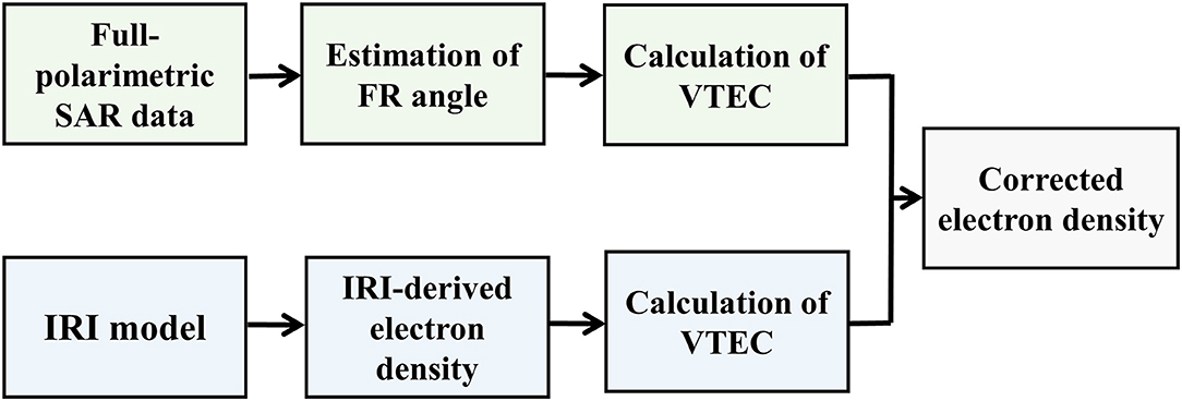
Figure 1. The flowchart of the proposed method.

Estimation of the FR Angle From SAR Images

For a linear polarization SAR system, the measured scattering matrix M can be written as follows (Freeman, 2004):

$\begin{array}{l}M=A{e}^{j\Phi }{R}^T{R}_{F}S{R}_{F}T+N\\ M=\left[\begin{array}{cc}{M}_{hh}& M_{vh}\\ M_{hv}& M_{vv}\end{array}\right],R_F=\left[\begin{array}{cc}\cos \Omega & \sin \Omega \\ -\sin \Omega & \cos \Omega \end{array}\right],S=\left[\begin{array}{cc}{S}_{hh}& S_{vh}\\ S_{hv}& S_{vv}\end{array}\right],\\ R^T=\left[\begin{array}{cc}1& {\delta }_1\\ {\delta }_2& f_1\end{array}\right],T=\left[\begin{array}{cc}1& {\delta }_3\\ {\delta }_4& f_2\end{array}\right],N=\left[\begin{array}{cc}{N}_{hh}& N_{vh}\\ N_{hv}& N_{vv}\end{array}\right]& (1)\end{array}$

where R_F is a one-way FR matrix; Ω is the FR angle; S is the true scattering matrix; R and T are the receiving and transmitting distortion matrices, respectively; f ₁ and f ₂ are the channel imbalance (the complex ratio of signals vertical (V)/horizontal (H) on receive and transmit, respectively); δ₁, δ₂, δ₃, δ₄ are the complex antenna crosstalk terms resulting from the incomplete isolation of H and V polarizations on transmit and receive; A is the overall gain of radar system, which is a function of radar range and elevation angle; e^jΦ corresponds to the roundtrip phase delay and system-dependent phase effects on signal; and N is an additive noise term due to earth radiation, thermal fluctuations in the receiver, and digitization noise (Freeman, 2004). A calibration technique applied to SAR data can correct the system-dependent terms of A, e^jΦ, R, and T in (1) (Meyer and Nicoll, 2008). Furthermore, filtering methods, such as boxcar, band-pass, and low-pass filters, can be used to suppress the additive noise N. After these calibrations, the measured scattering matrix M can be reformed as given by

$\begin{array}{ll}M=R_{F}S{R}_F& (2)\end{array}$

After expanding (2) and invoking true backscatter reciprocity (S_hv = S_vh), the components of matrix M can be defined as follows:

$\begin{array}{l}{M}_{hh}=S_{hh}{cos}^2\Omega -S_{vv}{sin}^2\Omega ,\\ M_{vh}=S_{hv}+(S_{hh}+S_{vv})sin\Omega cos\Omega ,\\ M_{hv}=S_{hv}-(S_{hh}+S_{vv})sin\Omega cos\Omega ,\\ M_{vv}=S_{vv}{cos}^2\Omega -S_{hh}{sin}^2\Omega & (3)\end{array}$

For cross-polarization, a non-zero FR angle means that the measured scattering matrix will not be invertible (M_vh ≠ M_hv). Suppose that FR angle is the only error source, and full-polarization SAR data is available, and then the FR angle can be easily estimated from (3). A robust algorithm has been proposed to estimate the FR angle through circular polarization scattering matrix Z (Bickel and Bates, 1965), as given by

$\begin{array}{ll}Z=\left[\begin{array}{cc}{Z}_{RR}& Z_{RL}\\ Z_{LR}& Z_{LL}\end{array}\right]=\left[\begin{array}{cc}1& j\\ j& 1\end{array}\right]\times \left[\begin{array}{cc}{M}_{hh}& M_{hv}\\ M_{vh}& M_{vv}\end{array}\right]\times \left[\begin{array}{cc}1& j\\ j& 1\end{array}\right]& (4)\end{array}$

$\begin{array}{ll}{Z}_{LR}=M_{vh}-M_{hv}+j\times (M_{hh}+M_{vv})& (5)\end{array}$

$\begin{array}{ll}{Z}_{RL}=M_{hv}-M_{vh}+j\times (M_{hh}+M_{vv})& (6)\end{array}$

From (3) and (4), FR angle Ω can be calculated by

$\begin{array}{ll}\Omega =-\frac{1}{4}\times \arg (Z_{RL}\times Z_{LR}^{*}),for-\frac{\pi }{4}<\Omega <\frac{\pi }{4}& (7)\end{array}$

where arg denotes the argument of a complex number, and ^* represents the complex conjugate. From (7), estimation of the FR angle becomes a phase estimation problem, which is a well-understood problem in radar polarization. Further, a reduction in noise is required in order to increase the quality of FR angle estimation. Some filtering methods can be used for the reduction.

Estimation of VTEC Distribution From SAR Images

The magnitude of FR angle Ω, for a wave of frequency f , traveling vertically one way through the ionosphere can be expressed as (Quegan and Lamont, 1986):

$\begin{array}{l}\Omega =\frac{\left|e^3\right|}{8{\pi }^{2}c{\epsilon }_0{m}^2}·\frac{\overline{B·cos\theta ·sec\varphi }·VTE{C}_{SAR}}{f^2}\\ =\frac{2.365\times 10^4·\overline{B·cos\theta ·sec\varphi }·VTE{C}_{SAR}}{f^2}& (8)\end{array}$

where e and m are the charge and mass of an electron, respectively; c is the speed of light; ε₀ is the permittivity of free space; B is the intensity of earth's magnetic field, which can be calculated from geomagnetic field data, such as international geomagnetic reference field (IGRF) data; θ is the angle between the magnetic field and satellite pointing vector; ϕ is the SAR incidence angle; $\overline{B·cos\theta ·sec\varphi }$ is the magnetic field factor at a constant height (e.g., 400 km); and f is the radar frequency. Generally, the value of $\overline{B·cos\theta ·sec\varphi }$ depends on the geographic coordinates, orbit, and imaging geometry of satellite and can be calculated from Wright et al. (2003). Once the FR angle is determined by (7), SAR-derived VTEC_SAR is calculated by.

$\begin{array}{ll}VTE{C}_{SAR}=\Omega ·\frac{f^2}{2.365\times 10^4·\overline{B·cos\theta ·sec\varphi }}& (9)\end{array}$

Reconstruction of Three-Dimensional Electron Density

International Reference Ionosphere is an empirical model based on real observation data combined with various ionospheric patterns, which can provide of global ionospheric parameters, such as ionospheric electron density (Bilitza et al., 2017). After obtaining the electron density with different altitude from IRI model, the IRI-derived VTEC is calculated by

$\begin{array}{ll}VTE{C}_{IRI}={\displaystyle \sum _{h=H_{min}}^{H_{max}}}{N}_e(h)& (10)\end{array}$

where VTEC_IRI is the IRI-derived VTEC, N_e(h) is the electron density at an altitude of h km, H_min, and H_max is, respectively, the minimum and maximum altitude when calculating the VTEC_IRI, ∑represents the operation of summing. As an empirical model, the IRI-derived electron density and VTEC is strong dependence on the underlying database, which means that regions and time periods not well-covered by the database will result in diminished reliability of the model in these areas. Thus, the corrected electron density could be obtained through combing of SAR-derived VTEC and IRI model:

$\begin{array}{ll}\widehat{N_e}(h)=N_e(h)\times (1+\frac{\Delta VTEC}{VTE{C}_{IRI}})& (11)\end{array}$

$\begin{array}{ll}\Delta VTEC=VTE{C}_{SAR}-VTE{C}_{IRI}& (12)\end{array}$

where $\widehat{N_e}(h)$ is the corrected electron density at an altitude of h km, and ΔVTEC is the difference between SAR-derived VTEC and IRI-derived VTEC. The sum of the corrected electron density should be satisfied by

$\begin{array}{ll}{\displaystyle \sum _{h=H_{min}}^{H_{max}}}\widehat{N_e}(h)=VTE{C}_{SAR}& (13)\end{array}$

After this operation, the improved high-spatial-resolution three-dimensional ionospheric electron density is mapped.

Data Collection

Two L-band full-polarimetric ALOS-1/Phase Array L-band SAR (PALSAR) images acquired on August 6, 2010, and March 31, 2011, are collected in this experiment. Figure 2A and Table 1 show the coverage and parameters of these SAR images, respectively. Using the collected SAR data, the high-spatial-resolution FR angle and VTEC distribution are estimated at 21:05:47 (UT) on August 6, 2010, and 07:27:38 (UT) on March 31, 2011, respectively. Meanwhile, the IRI-derived electron density data at the SAR-acquired time are collected from the IRI-2016 empirical model, which is the latest version of IRI. To keep the spatial consistency between SAR and IRI data, the IRI-derived electron density map is resampled to the SAR geographical coordinate system. Once SAR-derived VTEC and IRI-derived electron density are ready, the corrected electron density is reconstructed by (11). Additionally, ISR-derived electron density data at SAR-acquired time are collected from Poker Flat Incoherent Scatter Radar (PFISR) system with purpose of validating the corrected electron density. The PFISR system, located in central Alaska (69°N, 147°W), provides of near-continuous electron density measurements obtained over a ~3-year period, 2010–2013 (Negale et al., 2018). Figures 2B,C show the comparison of electron density between IRI and ISR on August 6, 2010, and March 31, 2011, respectively. It is observed that they are not always consistent, particularly for Figure 2C. As mentioned previously, this inconsistency is mainly due to the lack of enough underlying database for IRI to calculate the electron density.

FIGURE 2

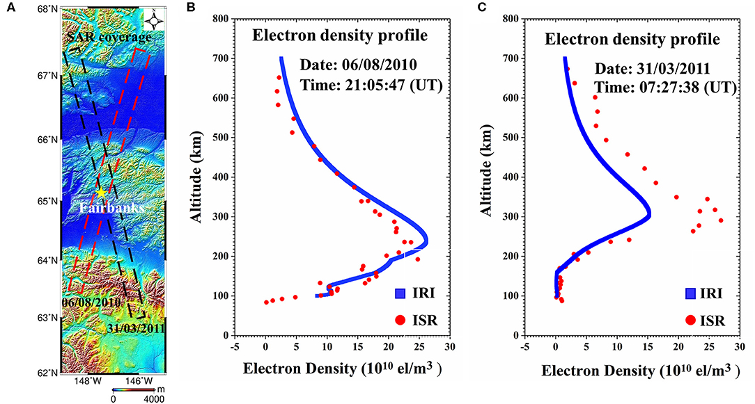
Figure 2. The collected datasets in this study. (A) The SAR data, where the black and red rectangles display the spatial coverages of SAR images, and the yellow star shows the locations of incoherent scatter radar (ISR) station; the electron density profiles from IRI (blue points) and ISR (red points) observations at SAR-acquired time on August 6, 2010 (B), and March 31, 2011 (C).

TABLE 1

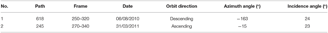
Table 1. Parameters of synthetic aperture radar (SAR) data in this study.

Experiment and Analysis

SAR-Derived FR Angle Distribution

For the collected SAR data with raw format (L0 level), they are processed to the single-look complex (SLC) format. During this procedure, the system-dependent terms of A, e^jΦ, R, and T in (1) are calibrated (Freeman, 2004; Meyer and Nicoll, 2008; Shimada et al., 2009). Then, measured scattering matrices M are formed from the full-polarimetric SLC data. The linear polarization scattering matrix M is transformed into circular polarized scattering matrix Z based on (4), and complex matrices of $Z_{LR}\times Z_{RL}^{*}$ are created. For suppressing the noises and preserving the same ground resolution in both of range and azimuth directions, multilooking operation of complex image with 2 looks in the range direction and 14 looks in the azimuth direction is applied to the $Z_{LR}\times Z_{RL}^{*}$. To reduce phase noise, the Goldstein adaptive filter with a window size of 32 is applied to the multilooked data (Baran et al., 2003). Finally, The SAR-derived FR angle maps on August 6, 2010, and March 31, 2011, are produced, as shown in Figure 3.

FIGURE 3

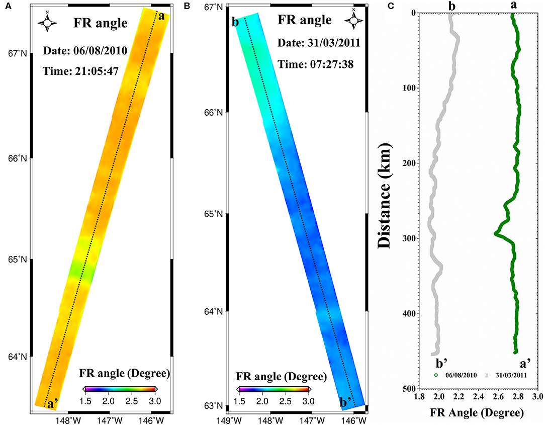
Figure 3. The SAR-derived FR angle maps on August 6, 2010 (A), and March 31, 2011 (B), where the FR angle profile along the lines a-a′ of (A) and b-b′ of (B) is shown in (C).

Figure 3A represents the spatial distributions of estimated FR angles on August 6, 2010. The statistics show that the mean value and standard deviation of FR angles are, respectively, 2.6° and 0.28° in Figure 3A. The small standard deviation suggests the absence of severe fluctuation of FR angles in space and relative quiet FR distribution over the study area. Because the system-dependent terms and noise have been calibrated and mitigated, the estimated FR angles in Figure 3A are primarily introduced by the ionosphere. Therefore, the relative quiet ionospheric activities are shown at the SAR-acquired time on August 6, 2010. However, careful inspection indicates that the subtle fluctuation appears in the lower-middle part of Figure 3A, which is clearly shown by the green line in Figure 3C. According to FR estimation theory in Estimation of the FR Angle From SAR Images, the FR may be affected by the calibration errors, such as inaccurate channel imbalance, crosstalk terms, additional noise, and backscatter characteristics of the imaged surface. In this case, the observed FR fluctuation in Figure 3A is considered to be related with the backscatter characteristics of the imaged surface through comparing the estimated FR distribution and ground surface types.

Figure 3B represents the spatial distributions of estimated FR on March 31, 2011. Compared to Figures 3A,B shows the smaller FR angles, where the mean value and standard deviation are, respectively, 1.9° and 0.19°. The smaller FR angle in Figure 3B may be related with the solar activity because it is ~10 o'clock in the evening at local time on March 31, 2011, whereas it is ~12 o'clock in the daytime at local time on August 6, 2010. It is similar with Figure 3A that the small standard deviation is observed in Figure 3B, indicating the relative quiet ionospheric activities at the SAR-acquired time on March 31, 2011. However, the FR gradient is observed in Figure 3B, which is clearly shown by the gray line in Figure 3C. Considering the gradient is varied with the latitude, we think the variations in Figure 3B are related with the geographical latitude.

Through analyzing the estimated FR angles, it is summarized that the relative quiet FR angles are shown at the SAR-acquired time on August 6, 2010, and March 31, 2011, although the subtle fluctuation and gradient are observed over the study area.

SAR-Derived VTEC Distribution

Once FR angles are determined, the SAR-derived VTEC maps can be generated from (9). For this process, the geomagnetic field parameters are required. The 13th generation IGRF, which is a standard mathematical description of the Earth's main magnetic field, is used for this case. Using SAR acquisition time and area, the geomagnetic field parameters are extracted from the IGRF and projected to the SAR coordinate system. Then, the geomagnetic field factor $\overline{B·cos\theta ·sec\varphi }$ at an altitude of 400 km is calculated by using geomagnetic field and SAR imaging geometry. The final SAR-derived VTEC maps on August 6, 2010, and March 31, 2011, are shown in Figure 4.

FIGURE 4

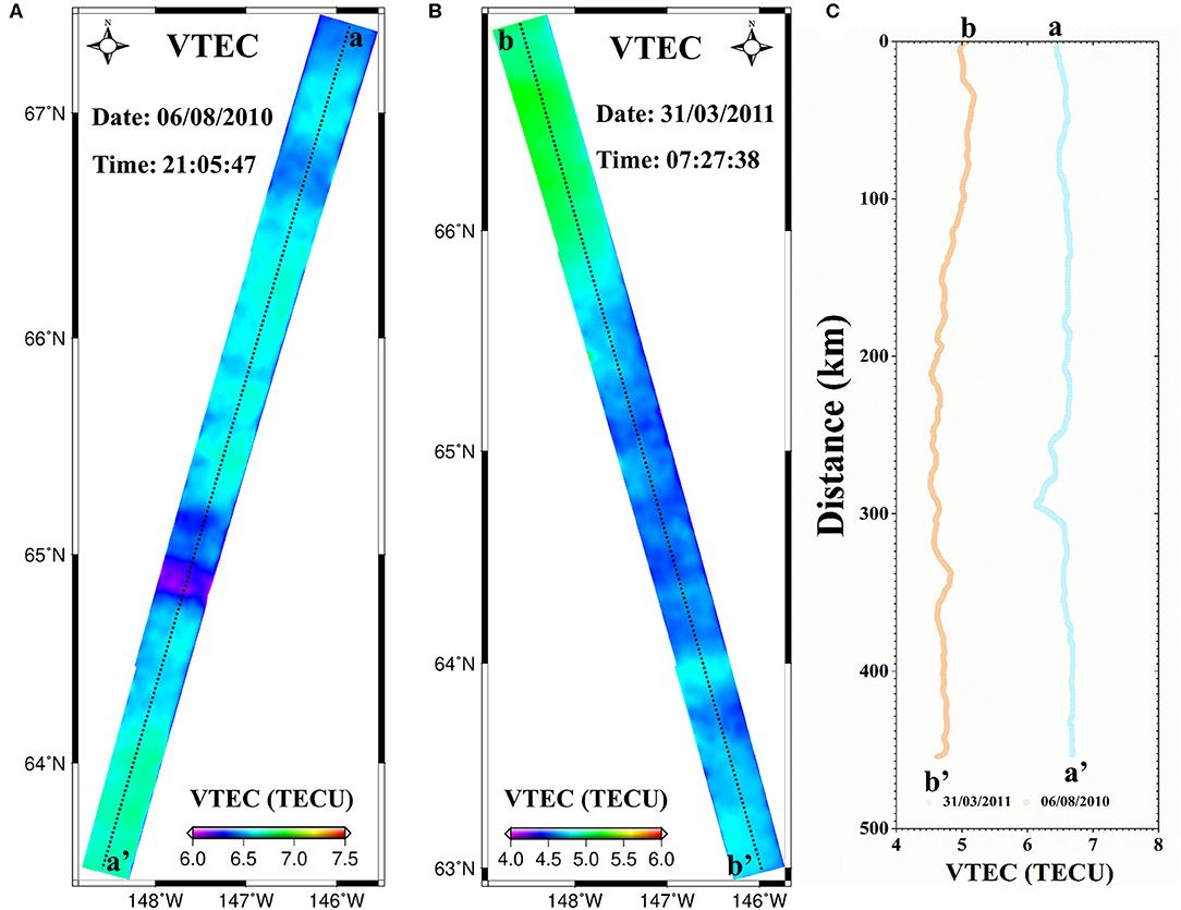
Figure 4. The SAR-derived VTEC maps on August 6, 2010 (A), and March 31, 2011 (B), where the VTEC profile along the lines a-a′ of (A) and b-b′ of (B) is shown in (C).

Figure 4A presents the spatial distributions of VTEC on August 6, 2010. It is observed that Figure 4A shows the similar spatial pattern with Figure 3A, suggesting that the geomagnetic field has little effect on the VTEC spatial variations. The statistics show that the mean value and standard deviation are, respectively, 6.3 and 0.67 TEC unit (TECU) in Figure 4A. The small standard deviation indicates the quiet ionospheric condition, which is sometimes known as the background ionosphere. The maximum VTEC in Figure 4A is ~6.7 TECU, which is located at the lowest latitude of SAR coverage. The minimum VTEC is ~6.2 TECU, which is located at lower-middle part of Figure 4A. The light blue line in Figure 4C, recording the VTEC values along the line aa' of Figure 4A, shows the ionospheric spatial variations along the latitude. It is found that the ionospheric activities display somewhat gradient and fluctuation in space.

Figure 4B presents the spatial distributions of VTEC on March 31, 2011. The mean value and standard deviation in Figure 4B are, respectively, 4.5 and 0.46 TECU, both of which are smaller than Figure 4A. These differences are due to the different imaging time for SAR observation. The small standard deviation indicates the background ionospheric condition over study area at the SAR-acquired time on March 31, 2011. The maximum and minimum VTEC are, respectively, 5.2 and 4.6 TECU, which are, respectively, located at the high and low latitude of SAR coverage. The prominent gradient is observed from the light brown line in Figure 4C, which records the VTEC values along the line b-b′ of Figure 4B. As analyzed in the last section, this gradient is related with the geographical latitude.

Based on the estimated VTEC, it is summarized that the study area belongs to the background ionosphere, where the mean VTEC values are 6.3 and 4.5 TECU on August 6, 2010, and March 31, 2011, respectively. Meanwhile, the ionospheric activities display somewhat gradient and fluctuation in space, rather than keep constant in space.

Three-Dimensional Electron Density

After extracting the electron density with different altitude, the IRI-derived VTEC at the SAR-acquired time and location is generated using (10). The difference between SAR-derived VTEC and IRI-derived VTEC is subsequently calculated and used to correct the IRI-derived electron density by (11). During this process, the electron density at different altitude is corrected and applied to each SAR pixel. Finally, the corrected three-dimensional ionospheric electron density maps on August 6, 2010, and March 31, 2011, are produced, as shown in Figures 5, 6. The Figure 7 presents the electron density along the lines a-a′ (marked in Figure 4A) and b-b′ (marked in Figure 4B).

FIGURE 5

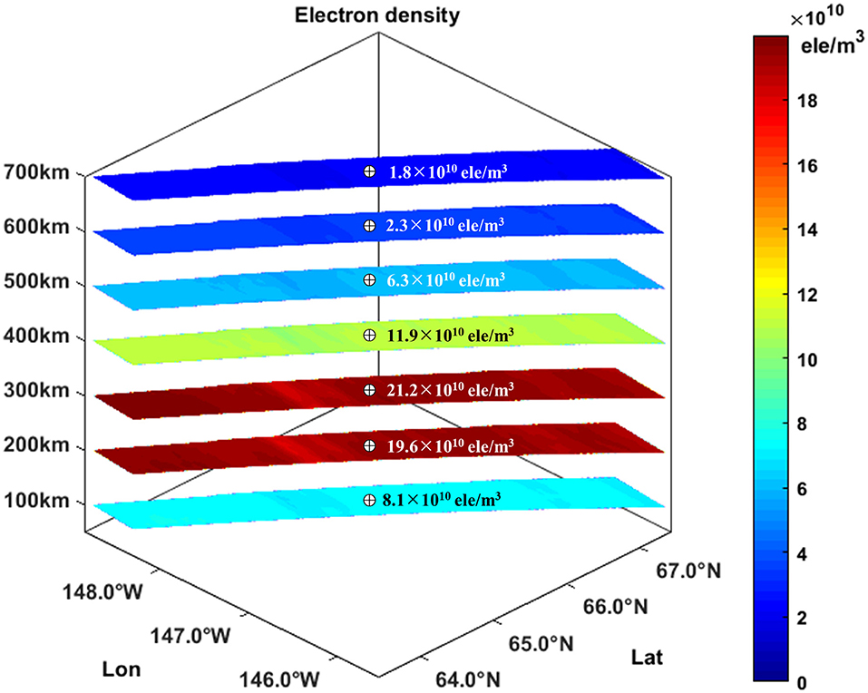
Figure 5. High-spatial-resolution three-dimensional ionospheric electron density on August 6, 2010, by combing of polarimetric SAR and IRI model, where cross circles represent the electron density at center of images.

FIGURE 6

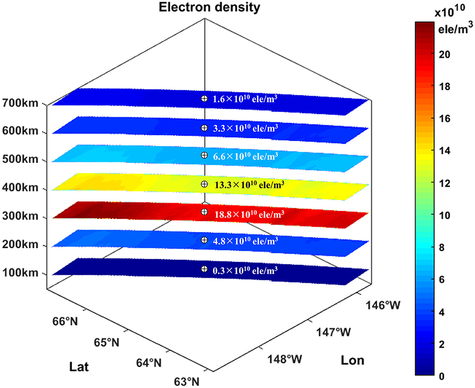
Figure 6. High-spatial-resolution three-dimensional ionospheric electron density on March 31, 2011, by combing of polarimetric SAR and IRI model, where cross circles represent the electron density at center of images.

FIGURE 7

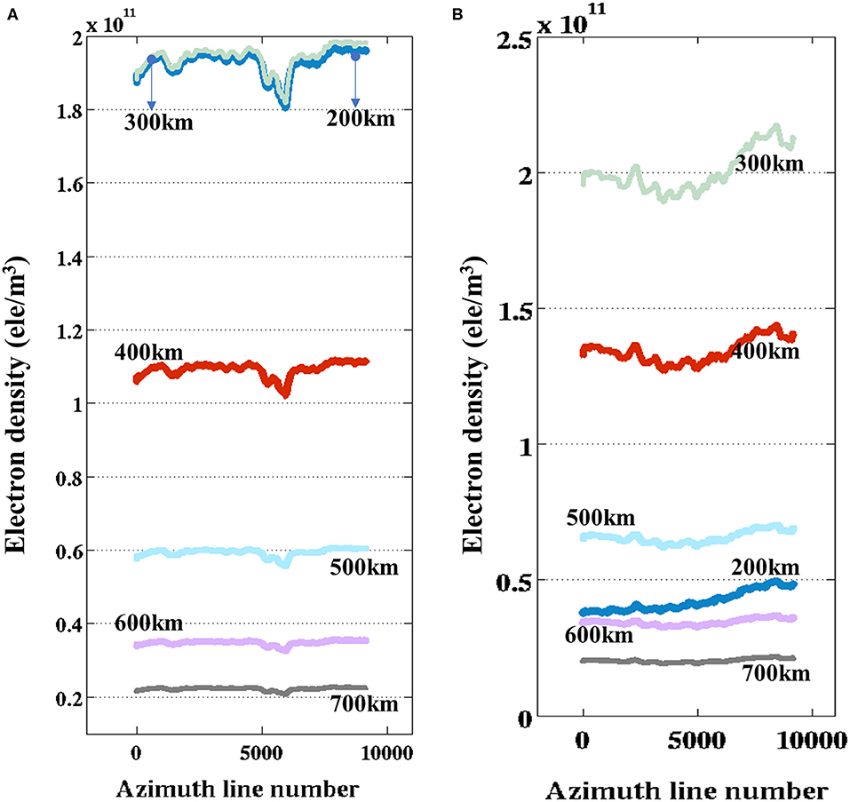
Figure 7. Profiles of electron density along the lines a-a′ of Figure 4A and b-b′ of Figure 4B at the different altitude on August 6, 2010 (A), and March 31, 2011 (B).

Figure 5 presents the ionospheric electron density at 100, 200, 300, 400, 500, 600, and 700 km above the ground on August 6, 2010. It is observed that the electron density increases followed by a decrease with the decreasing altitude and has a peak value of 24.6 ×10¹⁰ ele/m³ at an altitude of 238 km. Compared with Figure 2B, Figure 5 shows the similar electron density variations with IRI and ISR at the different altitude. In spatial domain, it seems that the electron density is nearly a constant at a certain altitude. However, further investigation shows that it presents the subtle fluctuation along the latitude. Figure 7A, recording the electron density at different altitude along the line a-a′ of Figure 4A, clearly displays the subtle fluctuation of electron density. Compared with the VTEC profile, it is found that the electron density in Figure 7A presents the similar variation pattern with the light blue line in Figure 4C.

Figure 6 presents the ionospheric electron density at 100, 200, 300, 400, 500, 600, and 700 km above the ground on March 31, 2011. Compared with Figure 5, the similar variation is presented in Figure 6: the electron density increases followed by a decrease with the decreasing altitude. However, the difference between them is that the maximum of electron density in Figure 6 is ~22.2 × 10¹⁰ ele/m³ at an altitude of 306 km. As mentioned previously, this difference is caused by the different SAR imaging time in Figures 5, 6. Figure 7B, recording the electron density at different altitude along the lines b-b′ of Figure 4B, displays the obvious gradient of electron density along the latitude. This gradient presents the similar variation pattern with the light brown line in Figure 4C.

In summary, the high-spatial-resolution three-dimensional electron density is estimated through integrating of SAR-derived VTEC and IRI model. The estimated electron density increases followed by a decrease with the decreasing altitude and has a peak value of 24.6 × 10¹⁰ ele/m³ at an altitude of 238 km on August 6, 2010, and 22.2 × 10¹⁰ ele/m³ at an altitude of 306 km on March 31, 2011.

The Comparisons of Electron Density From ISR, IRI, and Proposed Method

In order to validate the results, the electron densities from ISR, IRI, and proposed method are compared, as shown in Figure 8. The electron density of ISR at the SAR-acquired time and location (red circle in Figure 8) is collected from the PFISR system. The electron density of IRI (blue square in Figure 8) is collected from the IRI-2016 empirical model. The electron density of the proposed method (black triangle in Figure 8) is estimated through combing of polarimetric SAR and IRI model.

FIGURE 8

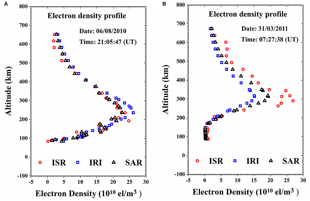
Figure 8. The comparisons of electron density from ISR, IRI, and proposed method at SAR-acquired time on August 6, 2010 (A), and March 31, 2011 (B).

Figure 8A shows the comparisons of electron density from ISR, IRI, and proposed method on August 6, 2010. It is observed that the electron density is consistent in shape and F2-layer peak height (hmF2) among ISR, IRI, and proposed method. For the shape, they present the increasing electron density followed by a decrease with the decreasing altitude. For the hmF2, the peak electron density is concentrated at an altitude of 238 km. Comparisons of the magnitude of electron density at different altitude suggest that IRI is close to ISR at most altitude except the around the altitude of hmF2, where the maximum difference of 3.55 × 10¹⁰ ele/m³ is observed. We think this inconsistency is mainly due to the lack of enough underlying database for IRI to calculate the electron density. Further comparisons of the electron density between proposed method and ISR at different altitude show that this inconsistency is mitigated, particularly around the altitude of hmF2. The statistics shows that the standard deviation of the differences between ISR and IRI in Figure 8A is about 2.13 × 10¹⁰ el/m³, whereas this value is decreased to 1.01 × 10¹⁰ el/m³ for the differences between ISR and proposed method. It means that the standard deviation decreases by approximately two times compared to those before the correction, demonstrating the reliability of the proposed method.

Figure 8B shows the comparison of electron density from ISR, IRI, and proposed method on March 31, 2011. It is similar with Figure 8A that the shape of electron density is approximately consistent among ISR, IRI, and proposed method. However, inconsistent hmF2 of electron density is observed in Figure 8B: the hmF2 is ~306 km for IRI and proposed method, whereas this value is ~289 km for ISR. The reason of same hmF2 between IRI and proposed method is that IRI is involved in the electron density estimation of proposed method. The inconsistent hmF2 between IRI and ISR may be due to the lack of enough underlying database for IRI empirical model. The standard deviation of the differences between ISR and IRI is ~3.95 × 10¹⁰ el/m³, whereas this value is decreased to 2.68 × 10¹⁰ el/m³ between ISR and proposed method. Approximately 1.5 times' decreases of standard deviation demonstrate the reliability of the proposed method. However, the improvement of electron density estimated by proposed method in Figure 8B is not significant as Figure 8A. We think this phenomenon may be caused by the inaccurate hmF2 from IRI model. Therefore, the hmF2 is also an important parameter when using the proposed method to estimate the electron density.

Based on the comparisons of electron density from ISR, IRI, and proposed method, the improvement of electron density is obtained through combing of polarimetric SAR and IRI model, demonstrating the reliability of the proposed method.

Conclusions

There are the difficulties in obtaining the high-spatial-resolution VTEC and three-dimensional electron density for the current methods and models. In this situation, this article presents an efficient method to retrieve the high-spatial-resolution VTEC and three-dimensional ionospheric electron density by combing of the full-polarimetric SAR and IRI model. For the performance test, two L-band ALOS/PALSAR full-polarimetric SAR images over Alaska regions are processed. Based on this study, the following conclusions are summarized:

(1) The VTEC distribution with high spatial resolution is successfully mapped from the full-polarimetric SAR data. In this study, the high-spatial-resolution VTEC distribution at SAR-acquired time is estimated from the FR angles, which help us better characterize the ionospheric spatial variation.

(2) Three-dimensional ionospheric electron density is successfully reconstructed by combing of the full-polarimetric SAR and IRI model. International Reference Ionosphere–derived electron density is corrected by the SAR-derived VTEC. When comparing with the electron density derived from PFISR system, it is found that the IRI-derived electron density is obviously improved, where the standard deviations of differences between PFISR and IRI decrease, respectively, by ~2 and 1.5 times compared to those before the correction, demonstrating the reliability of the developed method in reconstructing the three-dimensional ionospheric electron density.

Although the reliability of the proposed method has been proven by experiments, there are still two limitations. The first is the FR estimation error due to the inaccurate SAR calibration parameters, such as channel imbalance f1 and f2; crosstalk terms δ1, δ2, δ3, and δ4; additional noise N, as well as backscatter characteristics of the imaged surface. Because the SAR-derived VTEC is derived from the estimated FR, this error will inevitably introduce bias in the three-dimensional electron density reconstruction when using (11). The second is the three-dimensional electron density estimation error due to the inaccurate ionospheric parameters, such as hmF2 and E-layer parameters. Reconstructed electron density on March 31, 2011, is not as good as the result on August 6, 2010, which is mainly attributed to the inaccurate hmF2. Therefore, future research is needed in overcoming these limitations.

Data Availability Statement

The datasets generated for this study are available on request to the corresponding author.

Author Contributions

WZ, J-YC, and QZ contributed conception and design of the study. J-YC and J-MZ performed the data evaluation. WZ wrote the draft of the manuscript. WZ, J-YC, QZ, and J-MZ contributed to the interpretation of the data. All authors contributed to the article and approved the submitted version.

Funding

This research was funded by Chang'an university (Xi'an, China) through National Key R&D Program of China (2018YFC1505101 and 2019YFC1509802), Natural Science Foundation of China projects (NSFC) (Nos. 41941019, 41731066, 41790445, 41674001, and 41604001), Natural Science Basic Research Plan in Shaanxi Province of China (2018JQ4031 and 2018JQ4027), and the Fundamental Research Funds for the Central Universities, CHD (Nos. 300102269207 and 300102269303). This research was also funded by the Open Fund of Key Laboratory of Urban Land Resources Monitoring and Simulation, Ministry of Land and Resource (No. KF-2018-03-004).

Conflict of Interest

The authors declare that the research was conducted in the absence of any commercial or financial relationships that could be construed as a potential conflict of interest.

Acknowledgments

Several figures were prepared by using Generic Mapping Tools software. We are grateful to the reviewers for their constructive comments to improve this manuscript.

References

Baran, I., Stewart, M., Kampes, B., Perski, Z., and Lilly, P. (2003). A modification to the goldstein radar interferogram filter. IEEE Trans. Geosci. Remote Sens. 41, 2114–2118. doi: 10.1109/TGRS.2003.817212

CrossRef Full Text | Google Scholar

Belcher, D. P., Mannix, C. R., and Cannon, P. S. (2017). Measurement of the ionospheric scintillation parameter from sar images of clutter. IEEE Trans. Geosci. Remote Sens. 55, 5937–5943. doi: 10.1109/TGRS.2017.2717081

CrossRef Full Text | Google Scholar

Bickel, S. H., and Bates, R. H. T. (1965). Effects of magneto-ionic propagation on the polarization scattering matrix. Proc. IEEE 53, 1089–1091. doi: 10.1109/PROC.1965.4097

CrossRef Full Text | Google Scholar

Bilitza, D., Altadill, D., Truhlik, V., Shubin, V., Galkin, I., Reinisch, B., et al. (2017). International reference ionosphere 2016: from ionospheric climate to real-time weather predictions. Space Weather 15, 418–429. doi: 10.1002/2016SW001593

CrossRef Full Text | Google Scholar

Dautermann, T., Calais, E., Lognonn,é, P., and Mattioli, G. S. (2009). Lithosphere—atmosphere—ionosphere coupling after the 2003 explosive eruption of the soufriere hills volcano, montserrat. Geophys. J. Int. 179, 1537–1546. doi: 10.1111/j.1365-246X.2009.04390.x

CrossRef Full Text | Google Scholar

Davies, K., and Smith, E. K. (2002). Ionospheric effects on satellite land mobile systems. IEEE Antenn. Propag. M 44, 24–31. doi: 10.1109/MAP.2002.1167260

CrossRef Full Text | Google Scholar

Fattahi, H., Simons, M., and Agram, P. (2017). Insar time-series estimation of the ionospheric phase delay: an extension of the split range-spectrum technique. IEEE Trans. Geosci. Remote Sens. 99, 1–13. doi: 10.1109/TGRS.2017.2718566

CrossRef Full Text | Google Scholar

Freeman, A. (2004). Calibration of linearly polarized polarimetric SAR data subject to faraday rotation. IEEE Trans. Geosci. Remote Sens. 42, 1617–1624. doi: 10.1109/TGRS.2004.830161

CrossRef Full Text | Google Scholar

Galkin, I. A., and Reinisch, B. W. (2011). “Global ionospheric radio observatory (GIRO): status and prospective,” in IEEE General Assembly and Scientific Symposium (Istanbul). doi: 10.1109/URSIGASS.2011.6050896

CrossRef Full Text | Google Scholar

Hunsucker, R. D., and Hargreaves, J. K. (2007). The High-Latitude Ionosphere and its Effects on Radio Propagation. Cambridge, UK: Cambridge University Press.

Google Scholar

Jehle, M., Frey, O., Small, D., and Meier, E. (2010). Measurement of ionospheric TEC in spaceborne SAR data. IEEE Trans. Geosci. Remote Sens. 48, 2460–2468. doi: 10.1109/TGRS.2010.2040621

CrossRef Full Text | Google Scholar

Ji, Y., Zhang, Y., Zhang, Q., Dong, Z., and Yao, B. (2018). Retrieval of ionospheric faraday rotation angle in low-frequency polarimetric SAR data. IEEE Access 7, 3181–3193. doi: 10.1109/ACCESS.2018.2888928

CrossRef Full Text | Google Scholar

Kim, J. S., and Papathanassiou, K. (2014). “SAR observation of ionosphere using range/azimuth sub-bands,” in European Conference on Synthetic Aperture Radar (Berlin).

Google Scholar

Kuo, C. L., Huba, J. D., Joyce, G., and Lee, L. C. (2011). Ionosphere plasma bubbles and density variations induced by pre-earthquake rock currents and associated surface charges. J. Geophys. Res. Space 116, 1–10. doi: 10.1029/2011JA016628

CrossRef Full Text | Google Scholar

Le, H., Liu, J. Y., and Liu, L. (2011). A statistical analysis of ionospheric anomalies before 736 M6. 0+ earthquakes during 2002–2010. J. Geophys. Res. Space 116, 1–5. doi: 10.1029/2010JA015781

CrossRef Full Text | Google Scholar

Li, L., and Li, F. (2008). Ionosphere tomography based on spaceborne SAR. Adv. Space Res. 42, 1187–1193. doi: 10.1016/j.asr.2007.11.022

CrossRef Full Text | Google Scholar

Liu, J. Y., Chen, Y. I., Chuo, Y. J., and Chen, C. S. (2006). A statistical investigation of preearthquake ionospheric anomaly. J. Geophys. Res. Space 111, 1–5. doi: 10.1029/2005JA011333

CrossRef Full Text | Google Scholar

Liu, L., Le, H., Chen, Y., Zhang, R., Wan, W., and Zhang, S. R. (2019). New aspects of the ionospheric behavior over millstone hill during the 30-day incoherent scatter radar experiment in october 2002. J. Geophys. Res. Space 124, 6288–6295. doi: 10.1029/2019JA026806

CrossRef Full Text | Google Scholar

Maeda, J, Suzuki, T., and Furuya, M. (2016). Imaging the midlatitude sporadic E plasma patches with a coordinated observation of spaceborne InSAR and GPS total electron content. Geophys. Res. Lett. 43, 1419–1425. doi: 10.1002/2015GL067585

CrossRef Full Text | Google Scholar

Maltsev, Y. P., Leontyev, S. V., and Lyatsky, W. B. (1974). Pi-2 pulsations as a result of evolution of an alfvén impulse originating in the ionosphere during a brightening of aurora. Planet. Space Sci. 22, 1519–1533. doi: 10.1016/0032-0633(74)90017-8

CrossRef Full Text | Google Scholar

Mannix, C. R., Belcher, D. P., and Cannon, P. S. (2017). Measurement of ionospheric scintillation parameters from SAR images using corner reflectors. IEEE Trans. Geosci. Remote Sens. 55, 6695–6702. doi: 10.1109/TGRS.2017.2727319

CrossRef Full Text | Google Scholar

Mannucci, A. J., Iijima, B., Sparks, L., Pi, X., Wilson, B., and Lindqwister, U. (1999). Assessment of global TEC mapping using a three-dimensional electron density model. J. Atmos. Sol. Terr. Phys. 61, 1227–1236. doi: 10.1016/S1364-6826(99)00053-X

CrossRef Full Text | Google Scholar

Meyer, F., Bamler, R., Jakowski, N., and Fritz, T. (2006). The potential of low frequency SAR systems for mapping ionospheric TEC distributions. IEEE Geosci. Remote S 3, 560–564. doi: 10.1109/LGRS.2006.882148

CrossRef Full Text | Google Scholar

Meyer, F., and Nicoll, J. (2008). Prediction, detection, and correction of Faraday rotation in full-polarimetric L-band SAR data. IEEE Trans. Geosci. Remote Sens. 46, 3076–3086. doi: 10.1109/TGRS.2008.2003002

CrossRef Full Text | Google Scholar

Negale, M. R., Taylor, M. J., Nicolls, M. J., Vadas, S. L., Nielsen, K., and Heinselman, C. J. (2018). Seasonal propagation characteristics of MSTIDs observed at high latitudes over central alaska using the poker flat incoherent scatter radar. J. Geophys. Res. Space 123, 5717–5737. doi: 10.1029/2017JA024876

CrossRef Full Text | Google Scholar

Obayashi, T. (1962). Widespread ionospheric disturbances due to nuclear explosions during October 1961. Nature 196, 24–27. doi: 10.1038/196024b0

CrossRef Full Text | Google Scholar

Paula, E. R., and Hysell, D. L. (2004). The sao luis 30 MHz coherent scatter ionospheric radar: system description and initial results. Radio Sci. 39, 1–14. doi: 10.1029/2003RS002914

CrossRef Full Text | Google Scholar

Pedatella, N. M., Yue, X., and Schreiner, W. S. (2015). An improved inversion for FORMOSAT-3/COSMIC ionosphere electron density profiles. J. Geophys. Res. Space 120, 8942–8953. doi: 10.1002/2015JA021704

CrossRef Full Text | Google Scholar

Pi, X., Freeman, A., Chapman, B., Rosen, P., and Li, Z. H. (2011). Imaging ionospheric inhomogeneities using spaceborne synthetic aperture radar. J. Geophys. Res. Space 116, 1–13. doi: 10.1029/2010JA016267

CrossRef Full Text | Google Scholar

Quegan, S., and Lamont, J. (1986). Ionospheric and tropospheric effects on synthetic aperture radar performance. Int. J. Remote Sens. 7, 525–539. doi: 10.1080/01431168608954707

CrossRef Full Text | Google Scholar

Rosen, P. A., Hensley, S., and Chen, C. (2010). “Measurement and mitigation of the ionosphere in L-band interferometric SAR data,” in 2010 IEEE Radar Conference (Washington, DC), 1459–1463. doi: 10.1109/RADAR.2010.5494385

CrossRef Full Text | Google Scholar

Shimada, M., Isoguchi, O., Tadono, T., and Isono, K. (2009). PALSAR radiometric and geometric calibration. IEEE Trans. Geosci. Remote Sens. 47, 3915–3932. doi: 10.1109/TGRS.2009.2023909

CrossRef Full Text | Google Scholar

Takahashi, H., Costa, S., Otsuka, Y., Shiokawa, K., Monico, J. F. G., Paula, E., et al. (2014). Diagnostics of equatorial and low latitude ionosphere by TEC mapping over Brazil. Adv. Space Res. 54, 385–394. doi: 10.1016/j.asr.2014.01.032

CrossRef Full Text | Google Scholar

Wang, C., Guo, W., Zhao, H., Chen, L., Wei, Y., and Zhang, Y. (2019). Improving the topside profile of ionosonde with tec retrieved from spaceborne polarimetric SAR. Sensors 19:516. doi: 10.3390/s19030516

PubMed Abstract | CrossRef Full Text | Google Scholar

Wang, C., Zhang, M., Xu, Z. W., and Zhao, H. S. (2014). TEC retrieval from spaceborne SAR data and its applications. J. Geophys. Res. Space 119, 8648–8659. doi: 10.1002/2014JA020078

CrossRef Full Text | Google Scholar

Wang, R., Hu, C., Li, Y., Hobbs, S. E., and Chen, L. (2017). Joint amplitude-phase compensation for ionospheric scintillation in geo SAR imaging. IEEE Trans. Geosci. Remote Sens. 99, 1–12. doi: 10.1109/TGRS.2017.2672078

CrossRef Full Text | Google Scholar

Wright, P. A., Quegan, S., Wheadon, N. S., and Hall, C. D. (2003). Faraday rotation effects on L-band spaceborne data. IEEE Trans. Geosci. Remote Sens. 41, 2735–2744. doi: 10.1109/TGRS.2003.815399

CrossRef Full Text | Google Scholar

Yao, Y., Zhai, C., Kong, J., Zhao, Q., and Zhao, C. (2018). A modified three-dimensional ionospheric tomography algorithm with side rays. GPS Solut. 22, 1–18. doi: 10.1007/s10291-018-0772-4

CrossRef Full Text | Google Scholar

Zhu, W., Ding, X. L., Jung, H. S., Zhang, Q., Zhang, B. C., and Qu, W. (2016). Investigation of ionospheric effects on SAR Interferometry (InSAR): a case study of Hong Kong. Adv. Space Res. 58, 564–576. doi: 10.1016/j.asr.2016.05.004

CrossRef Full Text | Google Scholar