Spatial Distribution of Energy of Subinertial Baroclinic Motions in the Baltic Sea

Kurkin, Andrey; Rybin, Artem; Soomere, Tarmo; Kurkina, Oxana; Rouvinskaya, Ekaterina

doi:10.3389/feart.2020.00184

ORIGINAL RESEARCH article

Front. Earth Sci., 16 June 2020
Sec. Interdisciplinary Climate Studies
Volume 8 - 2020 | https://doi.org/10.3389/feart.2020.00184

Spatial Distribution of Energy of Subinertial Baroclinic Motions in the Baltic Sea

Andrey Kurkin¹^*

Artem Rybin¹

Tarmo Soomere^2,3

Oxana Kurkina¹

Ekaterina Rouvinskaya¹

¹Laboratory of Modeling of Natural and Anthropogenic Disasters, Nizhny Novgorod State Technical University n.a. R. E. Alekseev, Nizhny Novgorod, Russia
²Department of Cybernetics, School of Science, Tallinn University of Technology, Tallinn, Estonia
³Estonian Academy of Sciences, Tallinn, Estonia

We explore the basic properties of the “climate” of the field of subinertial motions with periods of 2–12 days in the Baltic Sea. The calculations are performed using the output of the Rossby Center Ocean Model RCO with a spatial resolution of 2 nautical miles for 1961–2005. The field of such motions in the Baltic Sea is strongly asymmetric, with much more energy present in the eastern regions of the sea. Spatial distributions of 5-yr average amplitudes of fluctuations of the main and seasonal pycnocline, near-bottom velocity and kinetic and potential energy reflect this asymmetry and also exhibit extensive variability on scales of a few tens of kilometers. The majority of potential energy of such motions is concentrated in a narrow nearshore strip of the sea with a typical width of <20 km. The largest values of kinetic energy occur along the gently sloping seabed at intermediate depths. The areas of maximum of absolute nearbed velocities only partially match similar areas hosting very large kinetic energy or strong fluctuations of the location of the pycnocline. Both the major properties and spatial details of the discussed distributions exhibit almost no difference for the years 1961–1965 and 2000–2005, except for the maximum seabed velocities that are somewhat larger in 2000–2005 apparently because of exceptional storms in 2001 and 2005.

Introduction

The well-being of the Baltic Sea ecosystem (e.g., in terms of eutrophication, Reissmann et al., 2009) and many details of the functioning of the entire sea (Leppäranta and Myrberg, 2009) substantially rely on the mechanisms that support strong vertical stratification in this water body. It is therefore natural that internal waves play a major role in the functioning of the entire sea. Their role is particularly large in the driving of mixing processes (Axell, 1998; Meier, 2001) and the formation of the vertical structure of its water masses (Axell, 2002; Lass et al., 2003), especially near the bottom slopes (Ozmidov, 1994). The importance of the impact of internal waves in this water body extends far beyond the classic dynamics and kinematics of motions in the sea and extends toward governing many major biochemical processes such as the formation and maintaining the anoxic zones or denitrification of the water column (Dalsgaard et al., 2013).

While the interplay of turbulence and internal waves is a generic issue in the coastal ocean (Burchard et al., 2008), the related aspects are particularly important in the Baltic Sea where steep vertical gradients often occur near the bottom. For example, about 30% of the energy needed for deep water mixing below the halocline in the Baltic Sea may be provided by the breaking of internal waves (Meier et al., 2006). The impact of internal waves is apparently significant for diapycnal mixing in the deep water of the Baltic Sea (Nohr and Gustafsson, 2009). It is also substantial in relatively sheltered but comparatively deep-water sub-basins such as the Gulf of Finland (Lilover and Stips, 2008, 2011).

The vertical structure of water masses of the Baltic Sea expresses the interplay of fresh water influx from the drainage area and water and salt exchange through the Danish straits. It leads to the presence of a strong relatively deeply located halocline and a relatively shallow seasonal thermocline in most parts of the sea (Leppäranta and Myrberg, 2009). The main density jump layer (pycnocline) is present permanently and usually lies at depths of about 60–80 m in the central part of sea called Baltic (Sea) proper. It is inter alia the most important waveguide for different scale baroclinic waves, including short-period internal waves, and a core channel of wave energy transfer between different parts of the sea. Its position indirectly affects the functioning of water masses in the medium-range depths of the sea through changing the kinematic and non-linear baroclinic wave properties (Talipova et al., 1998), supporting the generation, turning, and breaking of internal waves and associated intense mixing (Reissmann et al., 2009), and possible resuspension of bottom sediment (Friedrichs and Wright, 1995).

The main pycnocline and other jump layers are often located fairly close to the sea bottom of the Baltic Sea (Leppäranta and Myrberg, 2009) and in a number of locations even touch the seabed. Therefore, changes in the pycnocline depth may substantially relocate the typical areas of internal-wave-generated hydrodynamic loads and thus locations of intense resuspension of bottom sediment (e.g., Lundhansen and Skyum, 1992; Friedrichs and Wright, 1995; Bentley and Nittrouer, 1999). These changes also impact the associated conditions of sediment non-deposition favorable for the formation of ferromanganese concretions (Glasby et al., 1996) and indirectly affect large-scale infrastructure at the bottom. Even in areas that host large-scale quasi-stationary bottom gravity currents, relatively low-frequency motions with periods up to 30 min (that are possibly related to internal waves) strongly contribute to the bottom stress (Umlauf and Arneborg, 2009).

The related consequences are particularly extensive for the Baltic Sea (Massel, 2015). The usually existing three-layer structure supports specific types of non-linear internal waves (Kurkina et al., 2011a,b) in this basin. Moreover, changes to the properties of bottom mixed layers (Turnewitsch and Graf, 2003) or to the near-bottom hydrodynamic loads may adversely affect, e.g., chemical munitions dumped there after World War II (Beldowski et al., 2016) or govern the fate of new environmental agents such as plastic fibers with very low resuspension threshold (Bagaev et al., 2017).

The major properties of the most energetic (usually resonant) standing wave motions, their spatio-temporal distribution and frequency spectra in (semi-)enclosed basins are governed by the geometry, bathymetry and hydrology of the particular water body (Vlasenko et al., 2005). The basin-scale energy budget of the micro-tidal Baltic Sea is largely governed by two kinds of motions: inertial oscillations and low-mode near- and sub-inertial wave motions that are generated near the lateral slopes of the basin (van der Lee and Umlauf, 2011; Lappe and Umlauf, 2016). The properties of these motions are further modified by spatial inhomogeneities of stratification and water depth (Massel, 2015, 2016), reflections from the seabed, non-linear steepening, disintegration and breaking at the seabed and the nearshore, and various kinds of transformations (Rouvinskaya et al., 2015; Pelinovsky et al., 2018). The resulting motions are often extremely complicated and contain a multitude of different modes and types of motions. Resonance effects frequently play the core role in such processes (Friedrichs and Wright, 1995). They may amplify certain (long-wave) components of fluctuations or create energy cascade between different spectral components. The resulting resonant standing baroclinic waves can be a direct source of short-period internal waves, as well as affect the generation of internal waves by the wind (Whalen et al., 2018).

The properties of long barotropic and baroclinic wave phenomena and their signatures at sea surface are well-known for the Baltic Sea (Wübber and Krauss, 1979; Metzner et al., 2000; Kulikov et al., 2015). The predominant surface self-oscillations of the Baltic proper have periods around 27–29 hours. Their spatial structure and interrelations with seiches in other sub-basins of the Baltic Sea have been analyzed in detail in Jonsson et al. (2008). Less known are properties of large-scale baroclinic oscillations. Their approximate periods for the two lowest horizontal basin-scale modes for the Baltic Sea and its sub-basins lie in the range of 2–12 days. This time interval clearly exceeds the inertial period and is several times larger than the typical time scale of surface seiches in this water body (Leppäranta and Myrberg, 2009; Massel, 2015). The motions with these periods are usually not free waves. Zakharchuk and Tikhonova (2013) demonstrate that low-frequency motions have wave nature at a few locations at the margin of the deep-water Gotland Basin. Such motions still serve as effective means of (wave) energy exchange between different regions and eventually drive a multitude of processes on the shelves of medium-size water bodies such as the Baltic Sea or the Aral Sea (Roget et al., 2017). The associated waveguides are co-located with the main and seasonal pycnoclines. This kind of energy flux has been attributed, for example, to the development of sediment waves (Ribó et al., 2016), pockmarks (León et al., 2014) and large subaqueous sand dunes (Reeder et al., 2011) in other seas such as the Mediterranean Sea.

As baroclinic and internal waves propagate at much lower speeds than long surface waves (Massel, 2015), “internal wave storms” arrive remote areas much later than surface waves or oscillations of sea level. Moreover, their impact is often hidden and/or acts in a certain range of depths that is dictated by the specific combination of the local vertical stratification and the arriving internal wave field. Similarly to the surface wave climate, the field of such motions is a strong source of remote impact in the sense that the location of the largest hydrodynamic loads is separated from the typical generation area of such oscillations.

In this paper we analyze the main properties of long-period subinertial baroclinic motions in the Baltic Sea. The focus is on phenomena with periods in the range of 2–12 days. The analysis relies on numerically simulated properties of water masses in this water body in 1961–2005. The structure of the paper is as follows. Section Data and Methods shortly describes the circulation model, its output data set and the method for the calculations of the spectral properties of the field of subinertial baroclinic motions. Section Results focuses on the analysis of spectral properties of fluctuations of the main and seasonal pycnocline and spatial distributions of near-bottom velocities and kinetic and potential energy of the motions in this range of periods. Section Conclusions and Discussion reiterates the main conclusions and makes an attempt to put the results into the wider context of the entire Baltic Sea.

Data and Methods

Numerically Simulated Hydrographic Data

The analysis relies on time series of hydrological properties of the entire Baltic Sea produced by the Swedish Meteorological and Hydrological Institute (SMHI) using the Rossby Center Ocean Model RCO (Meier et al., 2003; Meier and Höglund, 2013) for May 1961–May 2005 and provided in the framework of BONUS BalticWay cooperation (Soomere et al., 2014). This 3D circulation model has been designed for simulations with moderate spatial resolution over long time intervals for studies of climate changes. The underlying equations (see detailed implementation, e.g., in Meier et al., 2003; Meier, 2007; Meier and Höglund, 2013) are solved on a regular rectangular grid (2 × 2 nautical miles) in the horizontal plane and using up to 41 vertical levels with thicknesses of 3–12 m in z-coordinates. Subgrid mixing is parameterized using the k–ε turbulence closure (Meier, 2001). The transport scheme embeds a flux-corrected, monotonicity-preserving routine with no explicit horizontal diffusion. A splitting scheme uses 150 s for the baroclinic and 15 s for the barotropic timestep. The output is stored once in 6 h.

The RCO model takes into account inflow of fresh water from the major rivers and water exchange through the Danish straits. The model uses wind properties at the height of 10 m above sea level, air temperature and specific humidity at a height of 2 m, precipitation, total cloudiness and sea level pressure. The meteorological forcing used to drive the particular model run was derived from the ERA-40 re-analysis (Uppala et al., 2005) using a regional atmospheric model with a horizontal resolution of 25 km (Samuelsson et al., 2011). Winter conditions are replicated using a Hibler-type sea ice model (Hibler, 1979).

The skill of the model in terms of replication of various features with different spatial and temporal scales has been thoroughly studied. A detailed assessment of the replicated vertical profiles and time series against representative monitoring stations and observations from the Baltic Environmental Database (BED) is performed in Placke et al. (2018). The RCO model provides better quality of replication of temperature and salinity profiles than, e.g., the GETM (General Estuarine Transport Model) or MOM (Modular Ocean Model) (Placke et al., 2018). The seasonal cycle and variability of temperature and salinity are simulated close to observations. Simulated current velocities lie mainly within the standard deviation of the measurements at the two monitoring stations (10 years of Acoustic Doppler Current Profiler (ADCP) measurements in the Arkona basin and 5 years of mooring observations in the Gotland basin, Placke et al., 2018).

To further illustrate the accuracy of the RCO model, we also compared the output of this model with data from the World Ocean Database (WOD). We present here the comparison of the modeled and measured vertical profiles of temperature, salinity and density at selected 5 locations (Figure 1) and at different time instants. Since the data sources have different vertical resolution, we performed a linear interpolation of the data to calculate the correlation coefficients and an estimate of the dissimilarity between the modeled and measured data in term of the relative error

\begin{array}{l} ε_{r e l} = \frac{| R C O_{v a l u e} - W O D_{v a l u e} |}{W O D_{v a l u e}} \cdot 100 % . & (1) \end{array}

An example of the match of the measured and modeled profiles at 20.583°E, 57.525°N on August 28, 1994 is presented in Figure 2. The modeled profiles follow well the measured one. The relevant correlation coefficients are 0.98 for temperature, 0.974 for salinity and 0.986 for density. The relative error is usually below 15% (<10% for density) and exceeds 30% only for temperature and salinity in a narrow range of depths at or near jump layers. For our purposes the most important feature is the match of modeled and measured profiles of density as this parameter is decisive for the properties of the medium in which internal waves propagate. The relevant values mostly differ by <5% (Figure 2). The largest difference (up to 15–20%) occurs at the lower margins of pycnoclines; however, the vertical structure of density and the depth, magnitude and thickness of the jump layers are fairly well represented.

FIGURE 1

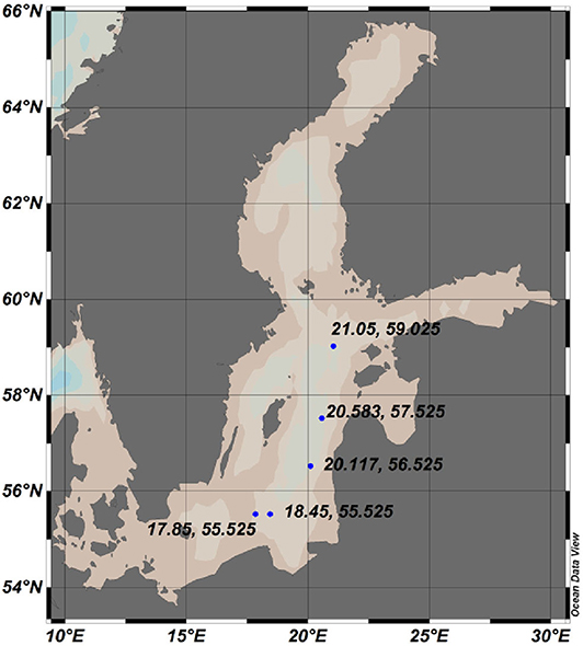
Figure 1. Locations of data points from the World Ocean Database used for comparison with the output ot the RCO model.

FIGURE 2

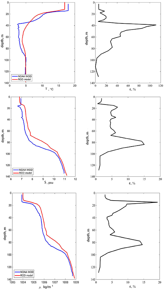
Figure 2. Temperature (T), salinity (S) and density (ρ) profiles from the World Ocean Database and from the RCO model, and the associated relative error (ε) at the location with coordinates 20.583°E, 57.525°N on August 28, 1994.

The largest shortages of the model are a too shallow halocline (Meier, 2007), problematic mixing during salt water inflows (Meier et al., 2003), and numerical noise affecting the sea surface temperature (Löptien and Meier, 2011). The mean circulation differs considerably between the models and due to the lack of current measurements only the baroclinic velocities can be compared with measured data (Placke et al., 2018). These problems insignificantly affect the results of our study.

The performance of the model to replicate processes with a time scale from hours up to few days has been evaluated in terms of water level. The time series and extremes of sea surface heights generally follow the measured values in the eastern Baltic Sea (except for a few locations that are affected by strong wave set-up, Eelsalu et al., 2014). This feature suggests that the model is suitable for the replication of processes with time scales of a few days. The trends in extreme water levels are also reproduced adequately for these measurement locations in the eastern Baltic Sea that well-represent offshore water level (Soomere and Pindsoo, 2016). Only storm surges in the western Baltic Sea are not always correctly replicated (Meier et al., 2004). The model resolves the major properties of mesoscale motions in the Baltic proper as well as the core changes in the vertical structure of water masses (Väli et al., 2013). It is therefore safe to say that the output of the model is suitable for the purposes of our study.

As mentioned above, a specific feature of water masses of the Baltic Sea is the presence of two density jump layers with comparable magnitudes. The spatial structure and temporal course of these layers are clearly resolved by the RCO model. The uppermost mostly mixed layer naturally exists in the entire sea. Its salinity is almost zero in the northernmost Gulf of Bothnia and easternmost Gulf of Finland, and has typical values of 7–8 g/kg in large parts of the sea. The temperature of this layer varies from almost zero to >20°C.

Near-bottom water masses (and thus the main pycnocline) spread only over deeper parts of the sea and have typical salinity 10–21 g/kg and temperature in the range of 4–12°C. The intermediate layer has usually temperatures of 2–6°C (occasionally also below zero, Mohrholz et al., 2006) and salinity of 8–10 g/kg. It is formed via a long-term process of mixing of surface and near-bottom waters. Relatively intense mixing acts at times from the sea surface down to depths of 50–60 m where the main pycno/halocline prevents its further impact.

Variations in the Location of the Pycnoclines

We evaluated first the variations in the depth of the main pycnocline following similar calculations in Väli et al. (2013). A location scheme of points in the Baltic Sea selected for the analysis below is presented in Figure 3 (including location of a Swedish/HELCOM monitoring station BY31 at the deepest place in the Baltic Sea). The sea water density in the water column was calculated using the standard equation of state (Fofonoff and Millard, 1983) from the modeled temperature, salinity and the vertical location of the water parcels. The location of the main pycnocline was evaluated as the depth of the largest density gradient at depths ≥30 m. The evaluation was performed four times a day for locations where the total sea depth exceeded 60 m.

FIGURE 3

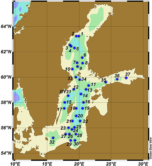
Figure 3. Location scheme of points in the Baltic Sea selected for the analysis.

The seasonal pycnocline in the upper layer of the sea (in which the local gradients may be even stronger than in the main pycnocline) was determined in a similar way but assumed to be not deeper than 30 m. The procedure resulted in discrete values of these two depths (corresponding to the relevant vertical levels in the RCO model) that varied all the way from surface to about 30 m depth level for the seasonal pycnocline and from 30 m depth level to the near-bottom layers for the main pycnocline. For the locations where the total depth was <60 m, the location of only the seasonal pycnocline was evaluated.

The largest variations in the location of the pycnoclines (Figure 4) reflect the seasonal course in the hydrological properties of water masses. The depth of the seasonal thermocline fluctuates considerably. It occasionally moves closer to the sea surface or even disappears owing to enhanced mixing during the windy (autumn and winter) season. Its location is much more stable and it deepens gradually during the relatively calm spring and summer seasons. These properties match the well-known features of the Baltic Sea stratification (Leppäranta and Myrberg, 2009). An exception was the year 2003 when the seasonal thermocline was located close to the sea surface during entire spring and most of summer.

FIGURE 4

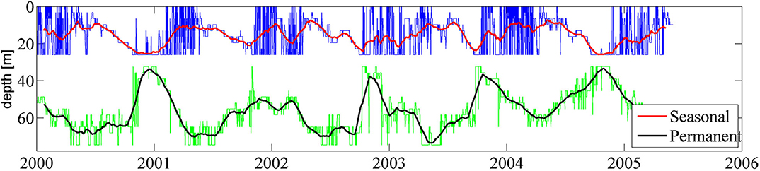
Figure 4. Vertical location of the seasonal (upper line) and main (permanent) pycnocline (lower line) 18.35°E, 58.01°N (point 23 in Figure 3) in 2000–2005. Thin lines represent the locations of the jump layer with a resolution of 6 h whereas the bold lines present the monthly moving average. Note that the restriction for the main pycnocline (below 30 m) and for the seasonal pycnocline to be located above this level may lead to an artificial separation of the two jump layers during certain time intervals (e.g., December 2001 or November 2005).

The main pycnocline behaves in counter-phase with respect to the seasonal one. It moves deeper in spring and is relocated closer to the sea surface in autumn so that in some years the main and seasonal pycnoclines eventually coalesced. However, the two clearly defined jump layers exist during most of the time and the water masses normally possess clear three-layer vertical structure in all parts of the sea where the main pycnocline exists. In particular, during the summer season the intermediate layer is quite thick. Consequently, the “symmetric” situation (with equal thicknesses of the uppermost and lowermost layers and the intermediate layer with a thickness twice as large as the other layers; Kurkina et al., 2011a) may persist in several locations of the sea for longer time intervals.

Vertically Integrated Kinetic and Potential Energy

We perform the analysis of spatial distribution of energy of baroclinic motions in terms of the relevant vertically integrated quantities. The core measures are (i) the fluctuations of vertical locations of the pycnoclines, (ii) near-bottom speed U and (iii) potential and (iv) kinetic energy in the entire water column per unit of sea surface. While vertical motions of the pycnocline to a large extent reflect the amplitude of internal waves and baroclinic motions, the other quantities involve also the impact of other motions of water masses. However, high near-bottom speeds are often associated with intense internal waves or other baroclinic motions. We employ the classic expressions for the kinetic (E_k) and potential (E_p) energy in this study:

\begin{array}{l} E_{p} (x, y, t) = g \int_{0}^{H} ρ (x, y, z, t) (H - z) d z, & (2) \end{array}

\begin{array}{l} E_{k} (x, y, t) = \frac{1}{2} \int_{0}^{H} ρ (x, y, z, t) [u^{2} (x, y, z, t) + v^{2} (x, y, z, t)] d z . & (3) \end{array}

Here x, y are horizontal coordinates, z is the vertical coordinate, z = 0 corresponds to the undisturbed sea surface, H is the total water depth, t is time, ρ is the density of sea water and (u, v) are horizontal velocity components of water parcels.

The location of the main pycnocline correlates well (with a large negative correlation coefficient) with the near-bottom speed (Figure 5). This kind of correlation may reflect the seasonal intensification of the baroclinic motions. Also, it may mirror the impact of changes in the vertical structure of water masses on local properties of baroclinic motions and associated velocity fields. For example, it is expected that shallower near-bottom layers host to higher near-bottom speeds even if the energy of internal waves is the same.

FIGURE 5

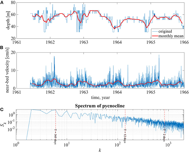
Figure 5. Temporal course of the location of the main pycnocline (A), near-bottom speed (B) and wavenumber spectra of fluctuations of the vertical location of the main pycnocline (C) at 18.25°E, 58.56°N (point BY31 in Figure 3). Thin lines in (A,B) panels show the course each 6 h. Bold lines represent moving average over 1 month.

Spectral Properties

We use spectral analysis to identify the spatial patterns and maxima and minima of the energy of motions in the range of periods of 2–12 days. The choice of the lower limit is dictated by the temporal resolution of the data set (6 h). The use of this sampling interval does not allow for an analysis of oscillations with periods shorter than 12 h. It is also desirable to implicitly exclude inertial motions and the signal of tides but still keep motions that correspond to relatively large energy in subbasins of the Baltic Sea (e.g., a secondary maximum at 8 h in the Gulf of Finland, see Sukhachev et al., 2014). Such an analysis is often used as a powerful tool to extract the predominant (resonant) modes or (eigen)oscillations of the basin. However, well-defined peaks of resonant modes are relatively infrequent and natural basins are more commonly characterized by wide peaks or gently sloping spectra. This is the situation also with slow motions in the Baltic Sea (Figure 5C). For this reason we address the entire field of motions in the discussed range of periods. The upper limit of 12 days, on the one hand, supports the propagation of wave energy over the entire Baltic Sea basin. On the other hand, it excludes the impact of certain specific basin-scale motions (e.g., major changes in the entire water volume of the Baltic Sea, see Lehmann et al., 2004; Lehmann and Post, 2015) on the outcome of the analysis.

The results of spectral analysis are presented below in terms of time-averaged spectral amplitudes A:

\begin{array}{l} A = T \int_{f_{l}}^{f_{u}} S (f) d f . & (4) \end{array}

Here f_l and f_u are the minimum and maximum frequencies of the chosen range of periods (2–12 days), the factor T corresponds to its length (10 days), and S(f) presents the discrete spectral amplitude for the discrete time series s_j of any quantity mentioned above:

\begin{array}{l} S_{k} = S (f_{k}) = \frac{| Ŝ_{k} |}{N}, Ŝ_{k} = \sum_{j = 1}^{N} s_{j} exp [- \frac{2 π i}{N} (j - 1) (k - 1)], & (5) \end{array}

N is the number of single values in the time series of s_j, $f_{k} = \frac{k F_{s}}{N}$ are the discrete frequencies, $F_{s} = \frac{1}{T_{s}}$ is the step in frequency space and T_s is the associated time interval, equal to the time step of the modeled hydrophysical data (6 h). As all quantities in Equation (4) are discrete, integration was performed using the simple trapezoidal rule. As we use the modeled values over almost half century but all existing measurements cover much shorter time periods, the calculated spectral amplitudes are not directly comparable with the ones extracted from measurements. However, given the demonstrated quality of the output of the RCO model (see the relevant references above), it is likely that the established qualitative patterns and areas that host high and low levels of different quantities are reliable.

Results

Fluctuations of the Main and Seasonal Pycnocline

We use spectral amplitudes of fluctuations of the seasonal pycnocline as a proxy of the intensity of the baroclinic motions. These amplitudes are the largest along a narrow strip along the eastern Baltic Sea coast from the Bay of Gdańsk until the entrance to the Gulf of Finland (in locations approximately 50 km from the shore), in the middle of the southern Baltic proper between Hel Peninsula and the island of Öland, along the eastern coast of the Sea of Bothnia and in the offshore of the southern part of this water body (Figure 6). The lowest levels of spectral amplitudes in question are found in the archipelago areas in the nearshore of Finland and western Estonia and, somewhat surprisingly, in the Arkona basin, Belt Sea and the Kattegat. The pattern is thus substantially anisotropic and reveals notable eastern intensification. The areas with large amplitudes of motions of the seasonal pycnocline are predominantly in the eastern nearshore of the entire Baltic Sea and the Sea of Bothnia.

FIGURE 6

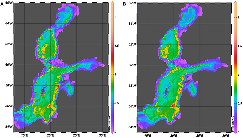
Figure 6. Spatial distribution of the spectral amplitude (Equation 4) of vertical fluctuations of the seasonal pycnocline (m) in 1961–1965 (A) and 2000–2005 (B).

Interestingly, the described pattern has almost no changes from the 1960s until 2000s (Figure 6). Even though the overall storminess in the Baltic Sea basin has not significantly altered since the 1880s (Hünicke et al., 2015), a substantial increase has occurred in the mean winter (December–January) wind speed in the entire Baltic Sea basin 1970–1995 (see, for example, Figure 4.10 of Rutgersson et al., 2015). Therefore, the overall stability of the established pattern is deeply non-trivial.

The calculations are performed in terms of spectral amplitudes of motions. The results thus characterize the average magnitude of motions over many years and, strictly speaking, cannot be directly associated with any particular phenomena. It is still likely that the revealed pattern to some extent reflects a regularly repeating configuration of baroclinic motions in the Baltic Sea. It qualitatively matches a typical picture of the amplitude distribution of standing oscillations of the lower basin-wide baroclinic mode with antinodes (amplitude maxima) in relatively shallow areas of the basin and nodal regions (with amplitudes close to zero) in central deeper parts of the sea. This pattern becomes evident not only in the Baltic proper but also in the Gulf of Finland, Sea of Bothnia, and Gulf of Bothnia. The relative amplitudes of the pycnocline fluctuations are much smaller in the subbasins than in the Baltic proper even though stratification in these subbasins is much weaker (Leppäranta and Myrberg, 2009).

Similar spectral amplitudes of fluctuations of the depth of the main pycnocline (Figure 7) represent only relatively deep areas where this jump layer is present during most of the time. Differently from the above, western intensification is observed. Namely, the areas with the most intense fluctuations (and thus with the largest baroclinic wave activity) are predominantly located near the western shores of the Baltic proper and the Sea of Bothnia, and in the Åland Sea. Only very small areas with comparable spectral amplitudes are found near the entrance of the Gulf of Finland (in an area to the north-west of the Western Estonian archipelago). If this pattern is interpreted as above (reflecting regularly repeating configuration of baroclinic waves or internal seiches), it may reflect frequently occurring baroclinic internal seiches with antinodes in the nearshore. This pattern in the Baltic proper seems to be strongly modified by the island of Gotland. Its presence seems to give rise to two separate structures whereas the nodal areas are more clearly localized.

FIGURE 7

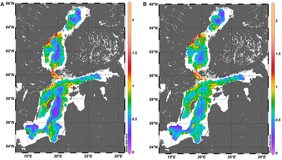
Figure 7. Spatial distribution of the spectral amplitude (Equation 4) of vertical fluctuations of the main pycnocline (m) in 1961–1965 (A) and 2000–2005 (B). The maximum value is 4.5 but for better readability the scale is limited to 2.25.

A combined spatial distribution of spectral amplitudes (Figure 8) reveals that the energy of baroclinic motions is inhomogeneously distributed along the nearshore of the Baltic Sea. The eastern and north-western coasts of the Baltic proper and most of the nearshore and offshore of the Sea of Bothnia host substantial activity of this sort of motions. As above, this pattern signals that these basins may have frequent internal (standing) oscillations with antinodes in these locations. The western coast of the Western Gotland Basin, the entire south-western part of the sea and smaller sub-basins (Gulf of Riga, Gulf of Finland and Bay of Bothnia) have much lower levels of spectral amplitudes of pycnocline fluctuations. This feature may interpreted as an indication of the frequent presence of nodes of such oscillations. This pattern is also basically the same for the 1960s and the 2000s.

FIGURE 8

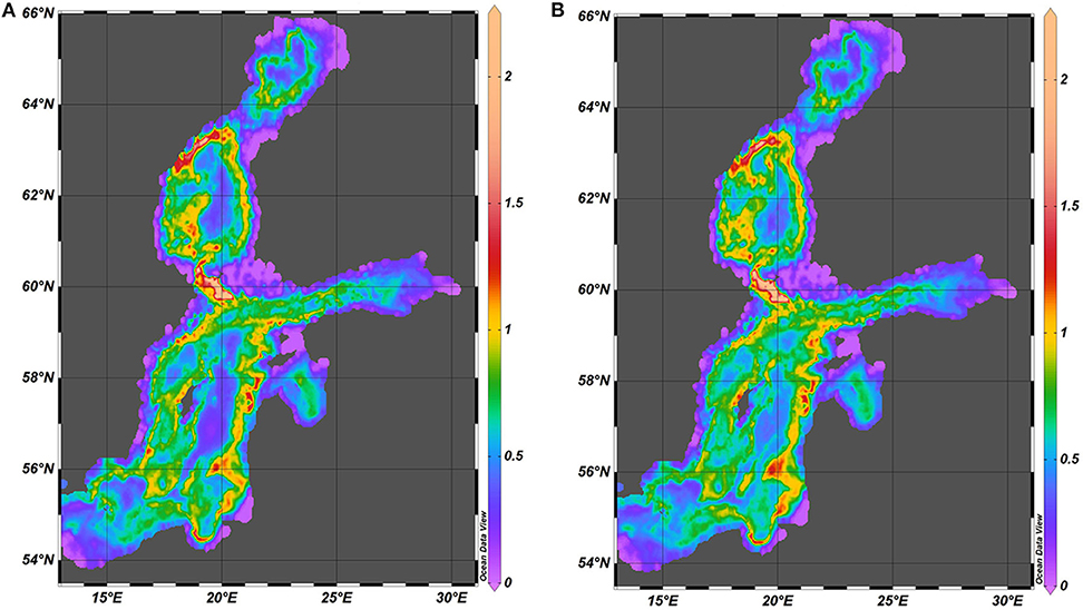
Figure 8. Spatial distribution of the combined spectral amplitude (Equation 4) of vertical fluctuations of pycnocline (m) in 1961–1965 (A) and 2000–2005 (B). The diagrams show this quantity for the main pycnocline in regions where it exists and the spectral amplitude for the seasonal pycnocline in the rest of the sea. The maximum value is 4.5 but for better readability the scale is limited to 2.25.

Near-Bottom Velocities

The distributions of maximum near-bottom velocities and their spectral amplitudes (Figures 9, 10) substantially differ from the above-discussed ones. The basin-wide pattern of high velocities resembles the pattern of large spectral amplitudes of vertical fluctuations of the main pycnocline. In both occasions high velocities systematically occur along the eastern nearshore of the Baltic proper and the Sea of Bothnia. The areas of high velocities are closer to the shore. This feature indicates a significant contribution to water velocities from surface waves (e.g., via wave-driven nearshore currents during long wave storms or relaxation of wave set-up events), wind-driven local currents and offshore circulation patterns.

FIGURE 9

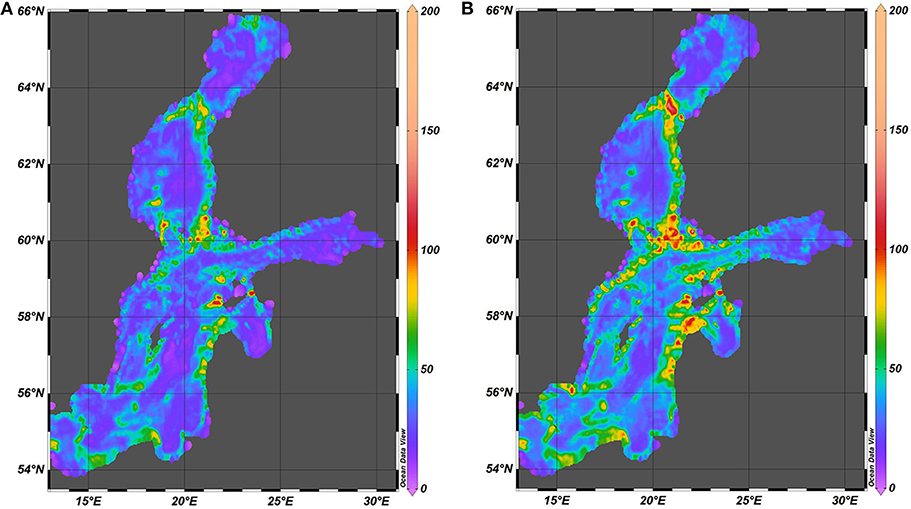
Figure 9. Spatial distribution of the maximum nearbed speed (cm/s) in 1961–1965 (A) and in 2000–2005 (B).

FIGURE 10

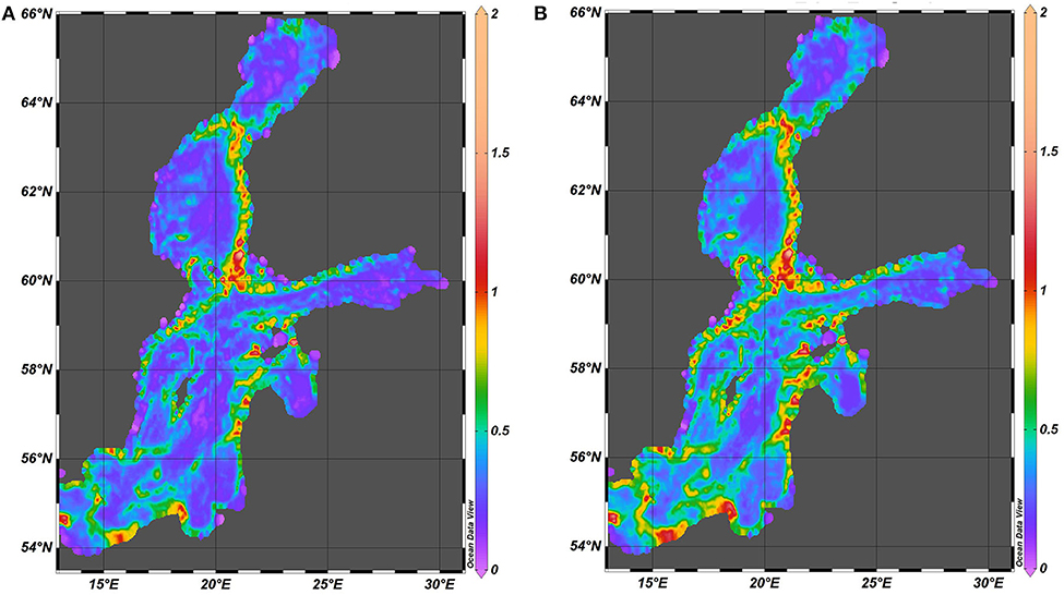
Figure 10. Spatial distribution of the spectral amplitude of nearbed speed (cm/s) in 1961–1965 (A) and in 2000–2005 (B).

The spatial distributions of velocities also have several considerably different features from those for fluctuations of pycnocline. The largest near-bottom velocities occur in specific spots located along sloping seabed. Large near-bed velocities may also occur in the Archipelago Sea between the Åland Islands and the Finnish mainland. It is likely that internal waves may be often generated in this area owing to shear flow through the deep channel between the Åland Islands and the Swedish mainland similarly to processes in the Gibraltar Strait (Vlasenko et al., 2009). The pattern of large near-bottom velocities only partially matches the spatial distribution of spectral amplitudes of near-bottom velocities (Figure 10). Both distributions suggest that the intensity of nearbed processes driven by baroclinic motions and internal waves is relatively low in the Gulf of Riga, Gulf of Finland and Bay of Bothnia compared to the open Baltic proper and the vicinity of Danish straits.

Even though some details and particular maximum values of nearbed velocities in 2000–2005 (Figure 9) are slightly different from those in 1961–1965, the spatial patterns of maximum velocities for these two time intervals almost exactly match each other. The single maxima in 2000–2005 are somewhat larger apparently because of a few unusually strong storms in 2001 and 2005. These storms created exceptionally large water levels in many sections of the eastern Baltic Sea coast (Suursaar et al., 2006). A substantial level of baroclinic motions and/or internal wave activity evidently was created during the relaxation phase of these events. The match of the relevant distributions for the two time intervals suggests that the locations where the internal waves and/or other baroclinic motions exert the strongest impact on the seabed in terms of high water velocities are governed by certain long-term combinations of the vertical structure of water masses and the appearance of seabed bathymetry.

Spatial Distributions of Potential and Kinetic Energy

Spatial distributions of spectral amplitude of potential energy normalized by the squared total depth (Figure 11) involve to some extent variations in the entire water level that may be largely driven by baroclinic perturbations (Zakharchuk et al., 2017). The spectral amplitudes in question thus provide another proxy of the intensity and frequency of baroclinic motions in this water body. Their distributions are substantially different from all distributions considered so far. Similarly to the above, these distributions for 1961–1965 and 2000–2005 almost exactly match each other. They are different from those discussed above first of all by a strong concentration of the majority of normalized potential energy of in a narrow nearshore strip of the sea with a typical width of <20 km. All deeper parts of the sea have much lower levels of normalized potential energy. These amplitudes (equivalently, the level of potential energy of the motions in question) substantially vary along the shoreline. The nearshore sections with the largest spectral amplitudes differ from similar locations for surface waves (e.g., Soomere and Räämet, 2011). This feature is not particularly surprising because refraction and transformation properties of baroclinic motions and internal waves greatly differ from similar (refraction and shoaling) properties of surface waves.

FIGURE 11

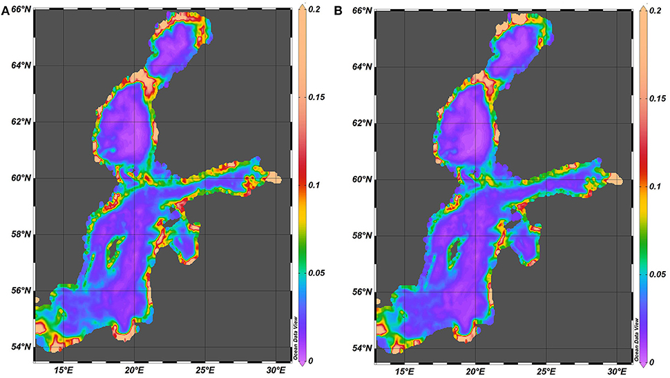
Figure 11. Spatial distribution of the normalized (1/H²) potential energy spectral amplitude (kg·s⁻²·m⁻²) in 1961–1965 (A) and 2000–2005 (B).

The kinetic energy of motions in Equation (3) also involves the energy of currents. It is therefore not surprising that it is distributed in a considerably different manner compared with the potential energy. The maxima of kinetic energy are located along sloping sections of the seabed around the deep areas in all basins of this water body (Figure 12). Very little kinetic energy is found in the deepest parts of the Baltic proper. The distribution has certain asymmetry: there is more kinetic energy in the eastern parts of the sea compared to the western parts. However, there is a visible correlation with the spatial distribution of the combined spectral amplitude of vertical fluctuations of the pycnocline (Figure 8).

FIGURE 12

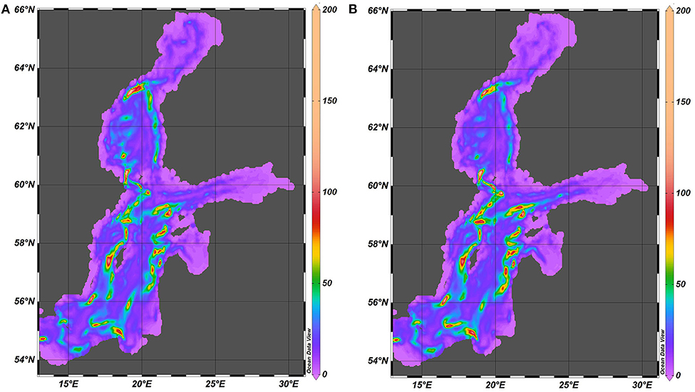
Figure 12. Spatial distribution of kinetic energy (kg·s⁻²) of internal waves in 1961–1965 (A) and 2000–2005 (B). The maximum value is 400 kg·s⁻² but for better readability the scale is limited to 200 kg·s⁻².

The levels of kinetic energy are much smaller in the Gulf of Riga and Gulf of Finland than in the Baltic proper or in the Sea of Bothnia. This feature is expected for the Gulf of Riga (that is separated from the Baltic proper by a sill) but somewhat surprising for the Gulf of Finland (that is widely open to the Baltic proper).

A comparison of the magnitudes of spectral amplitudes of kinetic energy and near-bottom velocities (Figure 13) indicates a strong dependence of the impact of water motions possibly driven by different phenomena on the seabed on a particular location. For relatively small depths (below 50 m), there is a significant scatter of kinetic energy relative to the near-bottom velocities. For larger depths these two quantities exhibit a power-law-like dependence of the form $E_{k} ~ U^{a}$ , a < 1.

FIGURE 13

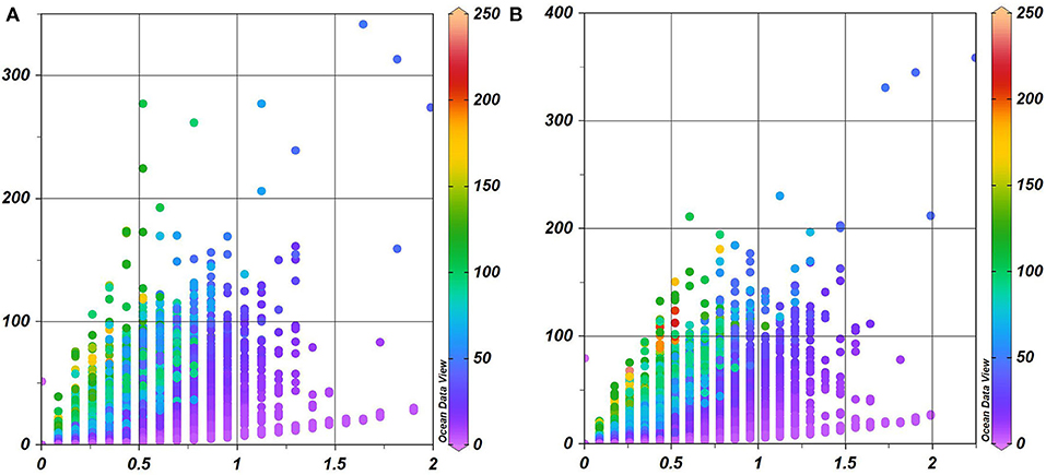
Figure 13. Scatterplots of spectral amplitudes of kinetic energy (vertical axis) and nearbed velocities (horizontal axis) in 1961–1965 (A) and 2000–2005 (B). Color scale indicates the water depth.

Conclusions and Discussion

The presented estimates of spatial distributions of the main parameters that characterize the long-term statistics of baroclinic motions in the period range of 2–12 days in 1961–2005 first of all suggest that the relevant field of motions in the Baltic Sea is highly inhomogeneous and strongly asymmetric. Interplay of the complicated geometry of the basin with its spatially and temporally varying stratification gives rise to extensive spatial variability of the associated quantities such as the typical amplitudes of fluctuations of the main and seasonal pycnocline, near-bottom velocity, and kinetic and potential energy. The variability extends from the basin scale down to scales on the order of about 10 km. This pattern matches well the perception that non-linear internal waves may change their appearance and kinematic properties along their usual pathways of propagation (Rouvinskaya et al., 2015) or that the internal wave dynamics on both sides of several sills (e.g., Slupsk Sill, Massel, 2016) may be different due to the different vertical density stratification in these areas.

Even though the results are presented in terms of certain statistical quantities (spectral amplitudes of motions over many years) and do not resolve single events, some of the established patters may reflect the systematic presence of certain motions. In particular, the spatial distributions of fluctuations of both pycnoclines resemble the similar distribution of standing oscillations with antinodes in relatively shallow areas and nodal regions in central parts of the sea. This pattern exists for the Baltic proper, Gulf of Finland, Sea of Bothnia, and Gulf of Bothnia.

Most of the normalized potential energy of motions in question is concentrated in a narrow nearshore strip of the sea with a typical width of <20 km. All deeper parts of the sea have much lower levels of this quantity. This result is not unexpected as the amplitude of baroclinic and internal waves that are generated in deeper waters generally increases when the water depth decreases. It is not surprising that the average amplitude of this quantity greatly varies along the shoreline. However, it is interesting that this variation does not follow the similar variation of wave heights (Soomere and Räämet, 2011) or onshore wave energy flux of surface waves (Soomere and Eelsalu, 2014).

The majority of kinetic energy is concentrated in a different region of the sea and thus apparently may be associated with other kinds of motions than baroclinic or internal waves. Namely, the eastern parts of the Baltic Sea along the gently sloping seabed at depths of about 20–40 m apparently are impacted by mesoscale and basin-scale currents that persist for a few days. Owing to strong non-linearity of such motions, these regions can serve as the main zones of generation of short-period internal waves (on the possible wave regimes, see: Kurkina et al., 2014). The areas of maximum nearbed velocities only partially match similar areas of very large kinetic energy or areas with the largest fluctuations of the pycnocline depth. This also not unexpected as the motions excited by baroclinic motions of the kind addressed in this paper are mostly concentrated in the vicinity of jump layers and only drive large near-bottom velocities if the bottom layer is thin or the wave is breaking. Therefore, it is necessary to take into account the particular appearance of the motion, its detailed characteristics and the local vertical structure of water masses for reliable estimates of its impact on the seabed.

The presence of several hot spots of hydrodynamic activity driven by baroclinic motions and quantified here in terms of near-bottom velocity (Figures 9, 10) is a principally new feature of the dynamics of the Baltic Sea. Such spots in regions with rocky bottom (mostly around the Åland Islands) may greatly contribute into the limitations and forcing factors of the local ecosystem but apparently do not strongly affect the dynamics of bottom sediment. Similar spots along the nearshore of Latvia (where the seabed predominantly consists of finer sediment) may change the current understanding of the stability and integrity of seabed in this area. It is commonly thought that the sediment properties and motions in the areas much deeper than the closure depth (about 6–7 m for this coastal stretch, Soomere et al., 2017) are basically determined by the properties of near-bottom motions driven by large-scale circulation and mesoscale features. Our results suggest that in several locations specifically the baroclinic and/or internal wave activity may be the main factor controlling the deposition and resuspension and affecting and shaping the features of the seabed.

Both the major properties and spatial details of the discussed distributions exhibit almost no difference for the years 1961–1965 and 2000–2005. Only the maximum seabed velocities are somewhat larger in 2000–2005 apparently because of exceptional storms in 2001 and 2005. This stability suggests that the clear changes in the external forcing (e.g., Soomere et al., 2015), including a substantial increase in the mean winter (December–January) wind speed in the entire Baltic Sea basin 1970–1995 (Rutgersson et al., 2015), and variations in the vertical structure of water masses (Väli et al., 2013) over the second half of the twentieth century have almost not influenced the discussed features of “climate” of baroclinic motions in the Baltic Sea.

Finally, we emphasize that the described features stem exclusively from model simulations. Even though the model itself has been extensively validated against hydrophysical data (Meier et al., 2004; Placke et al., 2018) and the quality of forcing fields has been estimated in detail (Placke et al., 2018), the level of uncertainty of the presented results remains an open question.

Data Availability Statement

The data analyzed in this study was obtained from the Swedish Meteorological and Hydrological Institute in the framework of the BONUS BalticWay initiative. The data are free for academic research purposes. Requests to access these datasets should be directed to Prof. H. E. Markus Meier (meier@io-warnemuende.de).

Author Contributions

AK, TS, and OK designed the study, supervised the entire process, developed the method for the analysis, provided the first interpretation of results, created test images, and drafted the body parts of the paper. AR extracted the necessary data from the RCO output data set and wrote most of the scripts for the analysis. TS drafted the introduction and discussion sections and wrote the description of the RCO model. AR and ER performed the analysis, created the images, and contributed to the drafting of the Results section. All authors participated in the final polishing of the manuscript and have accepted the submitted version of the manuscript.

Funding

This study was initiated in the framework of grants of the President of the Russian Federation (NSh-2485.2020.5 and SP-1225.2019.5), institutional block grant IUT33-3 of the Estonian Ministry of Education and Research, and the Flag-ERA project Large scale experiments and simulations for the second generation of FuturICT (FuturICT 2.0), Estonian Research Council grant 4-8/17/1.

Conflict of Interest

The authors declare that the research was conducted in the absence of any commercial or financial relationships that could be construed as a potential conflict of interest.

References

Axell, L. B. (1998). On the variability of Baltic Sea deepwater mixing. J. Geophys. Res.-Oceans 103, 21667–21682. doi: 10.1029/98JC01714

ORIGINAL RESEARCH article

Spatial Distribution of Energy of Subinertial Baroclinic Motions in the Baltic Sea

Introduction

Data and Methods

Numerically Simulated Hydrographic Data

Variations in the Location of the Pycnoclines

Vertically Integrated Kinetic and Potential Energy

Spectral Properties

Results

Fluctuations of the Main and Seasonal Pycnocline

Near-Bottom Velocities

Spatial Distributions of Potential and Kinetic Energy

Conclusions and Discussion

Data Availability Statement

Author Contributions

Funding

Conflict of Interest

References

This article is part of the Research Topic

People also looked at