Comparative Analysis of the Structures and Outcomes of Geophysical Flow Models and Modeling Assumptions Using Uncertainty Quantification

1. Introduction

This paper describes an uncertainty quantification driven approach to analyze total models and individual assumptions that are composed into models of geophysical mass flows. This is especially relevant when the observations/measurements are not adequate to characterize the behavior of the system which is modeled. Observational data inadequacy is rarely characterized even for verified and validated models.

Since models actualize a hypothesis, it follows that a model articulates a belief about the data. Thus a model will always have some uncertainty in prediction, since the subjectivity of the belief can never be completely eliminated (Higdon et al., 2004; Kennedy and O'Hagan, 2011), nor is the data at hand usually enough to characterize its behavior at the desired prediction. Principles like “Occam's razor” and Bayesian statistics (Farrell et al., 2015) provide some guidance, but robust and quantitative approaches that allow the testing of model components for fitness need to be developed. In related work, we have shown that the application of the empirical falsification principle (Popper, 1959) over an arbitrarily wide envelope of possible inputs reduces the subjectivity and uncertainty in a case study where the available data was not adequate (Bevilacqua et al., 2019).

There are usually numerous models for representing complex systems with sparse observations, like large scale geophysical mass flows (Kelfoun, 2011). It is often difficult to decide which of these models are appropriate for a particular analysis. Nevertheless, ready availability of many models as reusable software tools makes it the user's burden to select one appropriate for their purpose. For example, the 4^th release of TITAN2D¹, already adopted in Bevilacqua et al. (2019), offers multiple rheology options in the same code base (Simakov et al., 2019). The availability of different models for similar or the same phenomena in the same tool provides us the ability to directly compare outputs and internal variables in all the models while controlling for difficult to quantify effects like numerical solution procedures, input ranges and computer hardware. This can improve the process for integrating information from multiple models (Bongard and Lipson, 2007). Given a particular problem for which predictive analysis is planned, the information generated and its comparison to available observational data can be used to guide model choice and input space refinement (Bevilacqua et al., 2019). However, as we have discovered, such comparison requires a careful understanding of each model and its constituents and a well-organized process like that which we describe here for such a comparison. In this study, we focus on the comparison between models, more than on the input space refinement problem.

A modeling assumption is essentially a simple postulate framing direct relationships among quantities under study. Models are compositions of many such assumptions. The study of models is, thus, a study of these assumptions and their composability and applicability. For complex systems good models may contains needless assumptions that may be removed or a good assumption could greatly improve a different model. In practice, these are usually subjective choices, not data driven. Moreover, assumptions needed may change as the system evolves, making model choice more difficult (Patra et al., 2018a).

In this study, we analyze the general features that differ among models in a probabilistic framework, oriented to extrapolation and forecast. More significantly, we describe and compare them using newly introduced concepts of dominance factors and expected contributions. This type of analysis, enabled by our approach, allows us to quantitatively evaluate modeling assumptions and their relative importance.

2. Methods and Data Sources

The statistically driven method introduced in this study for analyzing complex models provides extensive and quantitative information. Geophysical flow modeling usually compares simulation to observation, and fits the model parameters using the solution of a regularized inverse problem. Nevertheless, this is not always sufficient to solve forecasting problems, in which the range of possible flows might not be limited to a single type and scale of flow. Our approach is different, and evaluates the statistics of a range of flows, produced by the couple $(M,{{P}}_M)$—i.e., a model M and a probability distribution for its parameters ${{P}}_M$. New quantitative information can solve classical qualitative problems, either model-model or model-observation comparison. The mean plot represents the average behavior of flows in the considered range, and provides the same type of output that is provided by a single simulation. Moreover, the uncertainty ranges generate additional pieces of information that often highlight the differences between the models.

2.1. Analysis Process

Following the approach in Patra et al. (2018a) and Bevilacqua et al. (2019), we define $(M(A),{{P}}_{M(A)})$, where A is a set of assumptions, M(A) is the model composed of those assumptions, and ${{P}}_M$ is a probability measure in the input space of M. In this study we are considering a measure ${{P}}_M$ defined through a prior choice of the input domain. In general, ${{P}}_M$ could be obtained after a calibration step, or become a single value after the solution of an inverse problem for the optimal reconstruction of a particular flow. This could reduce the predictive capabilities of the model, where we have to investigate the outcomes over a non-trivial and relatively wide input space. However, our approach can be easily implemented after a more careful input space refinement (e.g., Bevilacqua et al., 2019).

Our problem cannot be solved using classical sensitivity analysis (e.g., Saltelli et al., 2010; Weirs et al., 2012), which decomposes the variance of model output with respect to the input parameters. Indeed, model assumptions cannot be seen as input parameters, because they are related to the terms in the governing equations. These terms can be seen as random variables depending on the inputs, but they have an unknown probability distribution and are not independent. In the sequel we will define the new concepts of dominance factors and expected contributions to cope with this problem. Essentially, if the assumptions represent the atomic elements constituting the models, then the dominance factors will tell us which atomic element is the most important in the model, and the contributing variables will quantitatively determine the full atomic decomposition of the model, through space and time.

The investigation of contributing variables illustrates the impact of modeling assumptions. Furthermore, understanding which assumptions dominate, and by how much, is a key step toward enabling the construction of more efficient models for desired inputs. We summarize our analysis process in two steps.

Stage 1: Setup of Parameter Ranges

In this study, we assume:

$\begin{array}{l}{{P}}_M\left(p_1,\dots ,p_{N_M}\right)~{\displaystyle \underset{i=1}{\overset{N_M}{\otimes }}}Unif(a_{i,M},b_{i,M}),\end{array}$

where N_M is the number of parameters of M. This is not restrictive, and in case of correlation between the commonly used parameters ${({\widehat{p}}_j)}_{j=1,{\widehat{N}}_M}$, or non-uniform distributions, we can always define a function g such that $g\left[{(p_i)}_{j=1,N_M}\right]={({\widehat{p}}_j)}_{j=1,{\widehat{N}}_M}$, and the (p_i) are independent and uniformly distributed. In particular, we choose these parameter ranges trough an explorative testing for physical consistency of model outcomes and range of inputs/outcomes of interest, and using information collected from the literature. This step is critical, because if the statistical comparison is dominated by trivial macroscopic differences, it cannot focus on the rheology details. In the preparation of hazard analysis, expert elicitation processes can be used to ensure that the studies correctly account for all anticipated and possible flow regimes.

Stage 2: Simulations and Output Data Gathering

For each model M, we produce datasets of model inputs, contributing variables and model outputs. These concepts are introduced in Patra et al. (2018a), and briefly reported in Bevilacqua et al. (2019). The model outputs could be flow height, lateral extent, area, velocity, acceleration, and derived quantities such as Froude number Fr. In general they include any explicit outcome of the flow calculations. Instead, the contributing variables include quantities that are related to individual assumptions A_i, typically not observed in the outputs of the model. For example these could be values of different source terms in momentum balances of complex flow calculations, or dissipation terms, or inertia terms. We base our analysis on a Monte Carlo simulation, sampling the model inputs and producing a family of graphs for the expectation of the contributing variables and model outputs. We also include their 5th and 95th percentiles. The sampling technique of the input variables follows Patra et al. (2018a). It is based on the Latin Hypercube Sampling idea (McKay et al., 1979; Stein, 1987; Owen, 1992a; Ranjan and Spencer, 2014; Ai et al., 2016), and in particular, on the improved space-filling properties of the orthogonal array-based Latin Hypercubes (Owen, 1992b; Tang, 1993). The volume of output data generated is likely to be large but modern computing and data handling equipment readily available to most modeling researchers² in university and national research facilities are more than adequate.

2.2. Monte Carlo Process and Statistical Analysis

In this study, like in Bevilacqua et al. (2019), the flow range is defined by establishing boundaries for inputs like flow volume or rheology coefficients characterizing the models. Latin Hypercube Sampling is performed over [0, 1]^d where d depends on the number of input parameters. Those scale-less samples are thus linearly transformed to span the required intervals. Section 3.2 provides examples of Latin Hypercube design in the three models that are targets of this study, with respect to their commonly used parameters.

Through the Monte Carlo simulation, we calculate data for each sample run and each output or contributing variable f(x, t) described as a function of time on the elements of the computational grid. This analysis produces very large volume of data which then has to be processed utilizing statistical methods for summative impact.

We devise many statistical measures for analyzing the data, following the definitions in Patra et al. (2018a) reported in this study for the sake of completeness. In particular, let (F_i(x, t))_i=1,…,k be an array of force terms, where x ∈ R^d is a spatial location, and t ∈ T is a time instant. The degree of contribution of those force terms to the flow dynamics can be significantly variable in space and time, and we define the dominance factors [P_j(x, t)]_{j = 1, …, k}, i.e., the probability of each F_j(x, t) to be the dominant force. Those probabilities provide insight into the dominance of a particular source or dissipation term on the model dynamics. We remark that we focus on the modulus of the forces and hence we cope with scalar terms. It is also important to remark that all the forces depend on the input variables, and they can be thus considered as random variables. Furthermore, these definitions are general and could be applied to any set of contributing variables, and not only to the force terms.

Definition 1 (Dominance factors). Let (F_i)_i=1,…,k be random variables on $(\Omega ,{F},{{P}}_M)$. Then, ∀i, the dominant variable is defined as:

$\begin{array}{l}\Phi :={\displaystyle \underset{i}{max}}\left|F_i\right|.\end{array}$

In particular, for each j = 1, …, k, the dominance factors are defined as:

$\begin{array}{l}{P}_j:={{P}}_M\left\{\Phi =\left|F_j\right|\right\}.\end{array}$

We remark that the dominant variable Φ is also a random variable, and in particular it is a stochastic process parameterized in time and space. Moreover, we define the random contributions, an additional tool that we use to compare the different force terms, following a less restrictive approach than the dominance factors. They are obtained dividing the force terms by the dominant force Φ, and hence belong to [0, 1].

Definition 2 (Expected contributions). Let (F_i)_i=1,…,k be random variables on $(\Omega ,{F},{{P}}_M)$. Then, ∀i, the random contribution is defined as:

$\begin{array}{l}{C}_i:=\{\begin{array}{ll}\frac{F_i}{\Phi },& \text{if}\Phi \ne 0;\\ 0,& \text{otherwise}.\end{array}\end{array}$

where Φ is the dominant variable. Thus, ∀i, the expected contributions are defined by E[C_i].

Thus, for a particular location x, time t, and parameter sample ω, we have C_i(x, t, ω) = 0 if there is no flow or all the forces are null. The expectation of C_i is reduced by the chance of F_i being small compared to the other terms, or by the chance of having no flow in (x, t). Expected contributions are obtained after diving the force terms by the dominant variable Φ, which is an unknown quantity depending on time, location, and input parameters. We provide an additional result, further explaining the meaning of those contributions through the conditional expectation. The proof is an easy consequence of the rule of chain expectation.

Proposition 3. Let (F_i)_i=1,…,k be random variables on $(\Omega ,{F},{P})$. For each i, let C_i be the random contribution of F_i. Then we have the following expression:

$\begin{array}{l}E\left[C_i\right]={\displaystyle \sum _j}{P}_j𝔼\left[\frac{F_i}{|F_j|}|\Phi =|F_j|\right],\end{array}$

where $P_j:={P}\left\{\Phi =|F_j|\right\}$.

2.3. Modeling of Geophysical Mass Flows

Models that are computationally tractable are rarely able to capture the physics of the complex flow class of large scale dense granular avalanches. In addition, very often the only actual information available is the a posteriori deposit left by the flow, with sparse data and significant uncertainty affecting the mechanisms of flow initiation and propagation. This modeling task is challenging and the subject of continuing research. Due to intrinsic mathematical, physical, or numerical issues, models that appear to reproduce well the flows in certain conditions, may turn out to be poor in others. However, because of the high consequences of such flows, several models composed of different assumptions have been proposed. For example in (Iverson, 1997; Denlinger and Iverson, 2001, 2004; Iverson and Denlinger, 2001; Pitman et al., 2003; Iverson et al., 2004; de' Michieli Vitturi et al., 2019), the depth-averaged model was applied in the simulation of test geophysical flows in large scale experiments. Several studies were specifically devoted to the modeling of volcanic mass flows (Bursik et al., 2005; Kelfoun and Druitt, 2005; Macías et al., 2008; Kelfoun et al., 2009; Charbonnier et al., 2013). In fact, volcanos are great sources for a rich variety of geophysical flow types and provide field data from past flow events.

We first assume that the laws of mass and momentum conservation hold for properly defined system boundaries. After this, because these flows are typically very long and wide with small depth we assume their shallowness (Savage and Hutter, 1989). This enables the calculation of simpler and more computationally tractable equations, by integrating through the flow depth. Both these assumptions, conservation laws and shallowness, could be investigated with the procedure defined above. Nevertheless, there is much evidence in the literature for their validity and we do not test them in this study.

The depth-averaged Saint-Venant equations that result are:

$\begin{array}{r}\frac{\partial h}{\partial t}+\frac{\partial }{\partial x}(hū)+\frac{\partial }{\partial y}(h\bar{v})=0\\ \frac{\partial }{\partial t}(hū)+\frac{\partial }{\partial x}\left(h{ū}^2+\frac{1}{2}k{g}_z{h}^2\right)+\frac{\partial }{\partial y}(hū\bar{v})=S_x\\ \frac{\partial }{\partial t}(h\bar{v})+\frac{\partial }{\partial x}(hū\bar{v})+\frac{\partial }{\partial y}\left(h{\bar{v}}^2+\frac{1}{2}k{g}_z{h}^2\right)=S_y& (1)\end{array}$

Like in Patra et al. (2005), here the Cartesian coordinate system is aligned such that z is normal to the surface; h is the flow height in the z direction; hū and $h\bar{v}$ are respectively the components of momentum in the x and y directions; and the earth pressure coefficient k relates the lateral stress components, ${\bar{\sigma }}_{xx}$ and ${\bar{\sigma }}_{yy}$, to the normal stress component, ${\bar{\sigma }}_{zz}$. We remark that $\frac{1}{2}k{g}_z{h}^2$ is the contribution of depth-averaged pressure to the momentum fluxes. S_x and S_y are the sum local stresses: as described in Patra et al. (2018a) they include the gravitational driving forces, the basal friction force resisting to the motion of the material, and additional forces specific of rheology assumptions.

The class of assumptions that we specifically test in this study are the assumptions on the rheology of the flows. In particular they model the different dissipation mechanisms embedded in S_x, S_y, and that cause an abundance of models with much controversy on the most suitable model.

We will define our approach and illustrate it using three models for large scale mass flows incorporated in our large scale mass flow simulation framework TITAN2D (Patra et al., 2005, 2006; Yu et al., 2009; Aghakhani et al., 2016). The description of the models is summarized from Bevilacqua et al. (2019) and reported in this study for the sake of clarity. So far, TITAN2D has been successfully applied to the simulation of different geophysical mass flows with specific characteristics (Sheridan et al., 2005, 2010; Rupp et al., 2006; Charbonnier and Gertisser, 2009; Norini et al., 2009; Procter et al., 2010; Sulpizio et al., 2010; Capra et al., 2011). Several studies involving TITAN2D were also directed toward a statistical study of geophysical flows, focusing on uncertainty quantification (Dalbey et al., 2008; Dalbey, 2009; Stefanescu et al., 2012a,b), or on the more efficient production of hazard maps (Bayarri et al., 2009, 2015; Spiller et al., 2014; Ogburn et al., 2016; Tierz et al., 2018; Bevilacqua et al., 2019; Hyman et al., 2019; Rutarindwa et al., 2019).

In the three following sections, we summarize Mohr-Coulomb (MC), Pouliquen-Forterre (PF) and Voellmy-Salm (VS) models. Models based on additional heterogeneous assumptions are possible, either more complex (Pitman and Le, 2005; Iverson and George, 2014) or more simple (Dade and Huppert, 1998). We decided to focus on these three because of their popularity. Moreover, if the degree of complexity in the models is significantly different, model comparison should take that into account, but this is outside the purpose of this study (Farrell et al., 2015).

2.3.1. Mohr-Coulomb Model

Based on the long history of studies in soil mechanics (Rankine, 1857; Drucker and Prager, 1952), the Mohr-Coulomb rheology (MC) was developed and used to represent the behavior of geophysical mass flows (Savage and Hutter, 1989).

Shear and normal stress are assumed to obey Coulomb friction equation, both within the flow and at its boundaries. In other words,

$\begin{array}{ll}\tau =\sigma tan\varphi ,& (2)\end{array}$

where τ and σ are respectively the shear and normal stresses on failure surfaces, and ϕ is a friction angle. This relationship does not depend on the flow speed.

We can summarize the MC rheology assumptions as:

• Basal Friction based on a constant friction angle.

• Internal Friction based on a constant friction angle.

• Earth pressure coefficient formula depends on the Mohr circle (it can be 0 or ±1).

• Velocity based curvature effects are included into the equations.

MC equations

As a result, we can write down the source terms of the Equation (1):

$\begin{array}{l}{S}_x=g_{x}h-\frac{ū}{\Vert {\displaystyle \underset{~}{\bar{\text{u}}}}\Vert }\left[h\left(g_z+\frac{{ū}^2}{r_x}\right)tan({\varphi }_{bed})\right]\\ -h{k}_{ap}\text{ sgn\hspace{0.17em}}\left(\frac{\partial ū}{\partial y}\right)\frac{\partial (g_{z}h)}{\partial y}sin({\varphi }_{int})\\ S_y=g_{y}h-\frac{\bar{v}}{\Vert {\displaystyle \underset{~}{\bar{\text{u}}}}\Vert }\left[h\left(g_z+\frac{{\bar{v}}^2}{r_y}\right)tan({\varphi }_{bed})\right]\\ -h{k}_{ap}\text{ sgn\hspace{0.17em}}\left(\frac{\partial \bar{v}}{\partial x}\right)\frac{\partial (g_{z}h)}{\partial x}sin({\varphi }_{int})& (3)\end{array}$

Where, $\underset{~}{\bar{\text{u}}}=(ū,\bar{v})$, is the depth-averaged velocity vector, r_x and r_y denote the radii of curvature of the local basal surface. The inverse of the radii of curvature is usually approximated with the partial derivatives of the basal slope, e.g., 1/r_x = ∂θ_x/∂x, where θ_x is the local bed slope.

In our study, sampled input parameters are ϕ_bed, and Δϕ : = ϕ_int − ϕ_bed. In particular, we assumed Δϕ ∈ [2°, 10°] (Dalbey et al., 2008).

2.3.2. Pouliquen-Forterre Model

The scaling properties for granular flows down rough inclined planes led to the development of the Pouliquen-Forterre rheology (PF), assuming a variable frictional behavior as a function of Froude Number and flow depth (Pouliquen, 1999; Forterre and Pouliquen, 2002, 2003; Pouliquen and Forterre, 2002).

PF rheology assumptions can be summarized as:

• Basal Friction is based on an interpolation of two different friction angles, based on the flow regime and depth.

• Internal Friction is neglected.

• Earth pressure coefficient is equal to one.

• Normal stress is modified by a pressure force linked to the thickness gradient.

• Velocity based curvature effects are included into the equations.

An empirical friction law ${\mu }_b(\Vert \underset{~}{\bar{\text{u}}}\Vert ,h)$ is defined in the whole range of velocity and thickness. The expression changes depending on two flow regimes, according to a parameter β and the Froude number $Fr=\Vert \underset{~}{\bar{\text{u}}}\Vert /\sqrt{h{g}_z}$. The critical angles ϕ₁ and ϕ₂, and the quantities ${L},\beta$ are the parameters of the model. In particular, ${L}$ is the characteristic depth of the flow over which a transition between the angles ϕ₁ to ϕ₂ occurs. More details can be found in Bevilacqua et al. (2019).

PF equations

The depth-averaged Equation (1) source terms thus take the following form:

$\begin{array}{l}{S}_x=g_{x}h-\frac{ū}{\Vert {\displaystyle \underset{~}{\bar{\text{u}}}}\Vert }\left[h\left(g_z+\frac{{ū}^2}{r_x}\right){\mu }_b(\Vert {\displaystyle \underset{~}{\bar{\text{u}}}}\Vert ,h)\right]+g_{z}h\frac{\partial h}{\partial x}\\ S_y=g_{y}h-\frac{\bar{v}}{\Vert {\displaystyle \underset{~}{\bar{\text{u}}}}\Vert }\left[h\left(g_z+\frac{{\bar{v}}^2}{r_y}\right){\mu }_b(\Vert {\displaystyle \underset{~}{\bar{\text{u}}}}\Vert ,h)\right]+g_{z}h\frac{\partial h}{\partial y}& (4)\end{array}$

In our study, sampled input parameters are ϕ₁, Δϕ₁₂ : = ϕ₂ − ϕ₁, and β. In particular, we assumed $\Delta {\varphi }_{12}\in \left[10°,15°\right]$, and β ∈ [0.1, 0.85]. Moreover, ${L}$ is equal to 1dm (Pouliquen and Forterre, 2002; Forterre and Pouliquen, 2003).

2.3.3. Voellmy-Salm Model

The theoretical analysis of dense snow avalanches led to the VS rheology (VS) (Voellmy, 1955; Salm et al., 1990; Salm, 1993; Bartelt et al., 1999). Dense snow or debris avalanches consist of mobilized, rapidly flowing ice-snow mixed to debris-rock granules (Bartelt and McArdell, 2009). The VS rheology assumes a velocity dependent resisting term in addition to the traditional basal friction, ideally capable of including an approximation of the turbulence-generated dissipation. Many experimental and theoretical studies were developed in this framework (Gruber and Bartelt, 2007; Kern et al., 2009; Christen et al., 2010; Fischer et al., 2012).

The following relation between shear and normal stresses holds:

$\begin{array}{ll}\tau =\mu \sigma +\frac{\rho \Vert {\displaystyle \underset{\_}{\text{g}}}\Vert }{\xi }\Vert {\displaystyle \underset{~}{\bar{\text{u}}}}{\Vert }^2,& (5)\end{array}$

where, σ denotes the normal stress at the bottom of the fluid layer and g = (g_x, g_y, g_z) represents the gravity vector. The two parameters of the model are the bed friction coefficient μ and the velocity dependent friction coefficient ξ.

We can summarize VS rheology assumptions as:

• Basal Friction is based on a constant coefficient, similarly to the MC rheology.

• Internal Friction is neglected.

• Earth pressure coefficient is equal to one.

• Additional turbulent friction is based on the local velocity by a quadratic expression.

• Velocity based curvature effects are included into the equations, following a different formulation from the previous models.

VS equations

Therefore, the final source terms take the following form:

$\begin{array}{l}{S}_x=g_{x}h-\frac{ū}{\Vert {\displaystyle \underset{~}{\bar{\text{u}}}}\Vert }\left[h\left(g_z+\frac{\Vert {\displaystyle \underset{~}{\bar{\text{u}}}}{\Vert }^2}{r_x}\right)\mu +\frac{\Vert {\displaystyle \underset{~}{\text{g}}}\Vert }{\xi }\Vert {\displaystyle \underset{~}{\bar{\text{u}}}}{\Vert }^2\right],\\ S_y=g_{y}h-\frac{\bar{v}}{\Vert {\displaystyle \underset{~}{\bar{\text{u}}}}\Vert }\left[h\left(g_z+\frac{\Vert {\displaystyle \underset{~}{\bar{\text{u}}}}{\Vert }^2}{r_y}\right)\mu +\frac{\Vert {\displaystyle \underset{~}{\text{g}}}\Vert }{\xi }\Vert {\displaystyle \underset{~}{\bar{\text{u}}}}{\Vert }^2\right].& (6)\end{array}$

In our study, sampled input parameters are μ, and ξ. In particular, ξ uniform sampling is accomplished in log-scale. In fact, values of ξ between 250 and 4,000 m/s² have been described for snow avalanches (Salm, 1993; Bartelt et al., 1999; Gruber and Bartelt, 2007).

2.4. Contributing Variables

For analysis of modeling assumptions we need to record and classify the results of different modeling assumptions. In our case study, we focus on the right-hand side terms in the momentum equation and we call them RHS forces, or, more simply, the force terms. They are internal to the computation and rarely visible as a system output.

$\begin{array}{ll}{RHS}_1=\left[g_{x}h,g_{y}h\right],& (7)\end{array}$

it is the gravitational force term, it has the same formulation in all models.

The expression of basal friction force RHS₂ depends on the model:

$\begin{array}{l}{RHS}_2=-h{g}_{z}tan({\varphi }_{bed})\left[\frac{ū}{\Vert {\displaystyle \underset{~}{\bar{\text{u}}}}\Vert },\frac{\bar{v}}{\Vert {\displaystyle \underset{~}{\bar{\text{u}}}}\Vert }\right],\text{\hspace{0.17em}in MC model}.\\ {RHS}_2=-h{g}_z{\mu }_b(\Vert {\displaystyle \underset{~}{\bar{\text{u}}}}\Vert ,h)\left[\frac{ū}{\Vert {\displaystyle \underset{~}{\bar{\text{u}}}}\Vert },\frac{\bar{v}}{\Vert {\displaystyle \underset{~}{\bar{\text{u}}}}\Vert }\right],\text{\hspace{0.17em}in PF model}.\\ {RHS}_2=-h{g}_z\mu \left[\frac{ū}{\Vert {\displaystyle \underset{~}{\bar{\text{u}}}}\Vert },\frac{\bar{v}}{\Vert {\displaystyle \underset{~}{\bar{\text{u}}}}\Vert }\right],\text{\hspace{0.17em}in VS model}.& (8)\end{array}$

The expression of the force related to the topography curvature, RHS₃, also depends on the model:

$\begin{array}{l}{RHS}_3=-htan({\varphi }_{bed})\left[\frac{{ū}^3}{r_x\Vert {\displaystyle \underset{~}{\bar{\text{u}}}}\Vert },\frac{{\bar{v}}^3}{r_y\Vert {\displaystyle \underset{~}{\bar{\text{u}}}}\Vert }\right],\text{\hspace{0.17em}in MC model}.\\ {RHS}_3=-h{\mu }_b(\Vert {\displaystyle \underset{~}{\bar{\text{u}}}}\Vert ,h)\left[\frac{{ū}^3}{r_x\Vert {\displaystyle \underset{~}{\bar{\text{u}}}}\Vert },\frac{{\bar{v}}^3}{r_y\Vert {\displaystyle \underset{~}{\bar{\text{u}}}}\Vert }\right],\text{\hspace{0.17em}in PF model}.\\ {RHS}_3=-h\mu \left[\frac{ū\Vert {\displaystyle \underset{~}{\bar{\text{u}}}}\Vert }{r_x},\frac{\bar{v}\Vert {\displaystyle \underset{~}{\bar{\text{u}}}}\Vert }{r_y}\right],\text{\hspace{0.17em}in VS model}.& (9)\end{array}$

All the three models have an additional force term, having a different expressions and different meaning in the three models:

$\begin{array}{l}{RHS}_4=-h{k}_{ap}sin({\varphi }_{int})\left[\text{ sgn\hspace{0.17em}}\left(\frac{\partial ū}{\partial y}\right)\frac{\partial (g_{z}h)}{\partial y},\text{ sgn\hspace{0.17em}}\left(\frac{\partial \bar{v}}{\partial x}\right)\frac{\partial (g_{z}h)}{\partial x}\right],\\ \text{\hspace{1em}\hspace{1em}\hspace{1em}\hspace{1em}in MC model}.\\ {RHS}_4=g_{z}h\left[\frac{\partial h}{\partial x},\frac{\partial h}{\partial y}\right],\text{\hspace{0.17em}in PF model}.\\ {RHS}_4=-\frac{\Vert {\displaystyle \underset{~}{\text{g}}}\Vert }{\xi }\Vert {\displaystyle \underset{~}{\bar{\text{u}}}}{\Vert }^2\left[\frac{ū}{\Vert {\displaystyle \underset{~}{\bar{\text{u}}}}\Vert }\frac{\bar{v}}{\Vert {\displaystyle \underset{~}{\bar{\text{u}}}}\Vert }\right],\text{\hspace{0.17em}in VS model}.& (10)\end{array}$

These contributing variables can be analyzed locally and globally for discriminating among the different modeling assumptions. We remark that a complete representation of the model functional should include also the left hand side (LHS) terms. For instance, the lateral stress component k_ap could be influenced by bed and internal frictional coefficients, and it appears in the LHS terms (Gray et al., 1999; Pirulli et al., 2007). Our statistical approach could be easily extended to the LHS terms. We did not focus on them for the sake of simplicity.

Finally, we also study the spatial integrals defined by $F(t)={\int }_{{ℝ}^k}f({\displaystyle \underset{\_}{\text{x}}},t)d{\displaystyle \underset{\_}{\text{x}}}$, where dx is the area of the mesh elements. This provides a global view of the results and is complementary to the observations taken locally. For instance, by integrating the scalar product of source terms in the momentum balance and velocity we can compare the relative importance of modeling assumptions when we seek accuracy on global quantities.

3. Case Study and Results

Our case study is a pyroclastic flow down the SW slope of Volcán de Colima (MX)—an andesitic stratovolcano that rises to 3,860 m above sea level, situated in the western portion of the Trans-Mexican Volcanic Belt (Figure 1). Volcán de Colima has historically been the most active volcano in México (la Cruz-Reyna, 1993; González et al., 2002; Zobin et al., 2002).

FIGURE 1

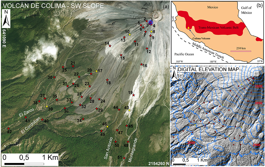
Figure 1. (a) Volcán de Colima (México) overview, including 51 numbered locations (stars) and major ravines. Initial pile is marked by a blue dot. Coordinates are in UTM zone 13N. (b) Regional geology map. (c) Digital elevation map. Six preferred locations are colored in yellow. Elevation isolines are displayed in blue, elevation values in red.

Pyroclastic flows generated by explosive eruptions and lava dome collapses of Volcán de Colima are a well-studied topic (Martin Del Pozzo et al., 1995; Sheridan and Macías, 1995; Saucedo et al., 2002, 2004, 2005; Sarocchi et al., 2011; Capra et al., 2015). The presence of a change in slope and multiple ravines characterize the SW slope of the volcano. Volcán de Colima has been used as a case study in several research papers involving the Titan2D code (Rupp, 2004; Rupp et al., 2006; Dalbey et al., 2008; Yu et al., 2009; Sulpizio et al., 2010; Capra et al., 2011; Aghakhani et al., 2016). On July 10th-11th, 2015, the volcano underwent its most intense eruptive phase since its Subplinian-Plinian 1913 AD eruption (Saucedo et al., 2010; Zobin et al., 2015; Capra et al., 2016; Reyes-Dávila et al., 2016; Macorps et al., 2018). We assume the flow to be generated by the gravitational collapse of a lava dome represented by a material pile placed close to the summit area—at 644956N, 2157970E UTM13 (Rupp et al., 2006; Aghakhani et al., 2016). A lava dome collapse occurs when there is a significant amount of recently-extruded highly-viscous lava piled up in an unstable configuration. Further extrusion and/or externals forces can cause the still hot dome of viscous lava to collapse, disintegrate, and avalanche downhill (Bursik et al., 2005; Wolpert et al., 2016; Hyman and Bursik, 2018). The volcano produced several pyroclastic flows of this type, called Merapi style flows (Macorps et al., 2018). The hot, dense blocks in this “block and ash” flow (BAF) will typically range from centimeters to a few meters in size.

The rheology of volcanic rock avalanches and dense pyroclastic flows is complex, and it is difficult to constrain the physics of the processes. A priori predictive ability of the known block and ash flow models is limited by inability to tune without knowledge of flow character (Patra et al., 2005). Since these dense flows are constituted of blocks, ash and gas, friction between the particles during emplacement could confer a Coulomb behavior to the whole flow. So, the Mohr Coulomb model was often considered appropriate, sometimes associated with a velocity or volume-dependent term (Spiller et al., 2014). However, a simple Coulomb behavior is not ideal, whatever the value of friction angle used. A friction angle that varies according to the velocity and thickness of the flows has also been assumed in the simulations of natural flows (Kelfoun, 2011). For these reason all three models, MC, VS and PF, are a priori appropriate but not ideal for a block and ash flow. Our new quantitative approach provides a tool in the evaluation of what model best characterizes the flow.

Our computations were performed on a DEM of 5m-pixel resolution, obtained from Laser Imaging Detection and Ranging (LIDAR) data acquired in 2005 (Davila et al., 2007; Sulpizio et al., 2010). We placed 51 locations along the flow inundated area to accomplish local testing. After evaluating the results in all the locations, six of them are adopted as preferred locations, being representative of different flow regimes.

3.1. Preliminary Consistency Testing of the Input Ranges

In this same setting, Dalbey et al. (2008) assumed ${\varphi }_{bed}=\left[15°,35°\right]$, while Capra et al. (2011) adopted ${\varphi }_{bed}=30°$. Then, Spiller et al. (2014) Bayarri et al. (2015), and Ogburn et al. (2016) found a statistical correlation between flow size and effective basal friction inferred from field observation of geophysical flows. A BAF at the scale of our simulations would possess ${\varphi }_{bed}=\left[13°,18°\right]$ according to their estimates. Small changes in the parameter ranges do not change significantly the results.

Figure 2 displays the maps of maximum flow height observed in the extreme cases tested. Simulation options are - max_time = 7,200 s (2 h), height/radius = 0.55, length_scale = 4 km, number_of_cells_across_axis = 50, order = first, geoflow_tiny = 1.0 × 10⁻⁴ (Patra et al., 2005; Aghakhani et al., 2016). Initial pile geometry is paraboloid. Even if the maximum runout is matched between the models, they display significantly different macroscopic features. In particular, MC displays a further distal spread before entering the ravines, PF shows a larger angle of lateral spread at the initiation pile, and stops more gradually than MC with more complex inundated area boundary lines. VS is less laterally extended and the material reaches higher thickness. The flow generally looks significantly channelized, and displays several not-inundated spots due to minor topographical coulées.

• Material Volume: [2.08, 3.12] × 10⁵ m³, i.e., average of 2.6 × 10⁵ m³ and uncertainty of ±20%.

• Rheology models' parameters:

MC - ${\varphi }_{bed}\in \left[10°,25°\right]$.

PF - ${\varphi }_1\in \left[8°,18°\right]$.

VS - μ ∈ [0.15, 0.45], log(ξ) ∈ [1.7, 4].

FIGURE 2

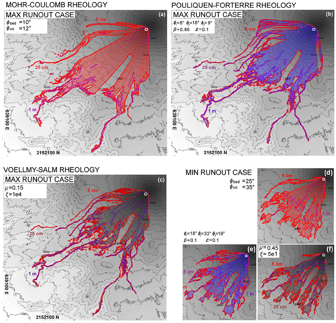
Figure 2. Volcán de Colima—comparison between max flow height maps of simulated flow, assuming MC (a,d), PF (b,e), and VS (c,f) models. Extreme cases—(a–c) max. volume–min. resistance and (d–f) min. volume–max. resistance.

We adopt a Latin Hypercube Sampling based on an orthogonal array OA(s^d, d, s, d) (Patra et al., 2018b). We take s = 8 for the 3-dimensional designs over the parameter space of Mohr-Coulomb and Voellmy-Salm models, i.e., 512 points; we took s = 6 for the 4-dimensional designs over the more complex parameter space of the Pouliquen-Forterre model, i.e., 1,296 points.

3.2. Exploring Flow Limits

Figures 3A–C illustrates the sampling design of our simulations. Figures 3D–I show examples of the contributions obtained assuming parameter values at the extremes of their range.

FIGURE 3

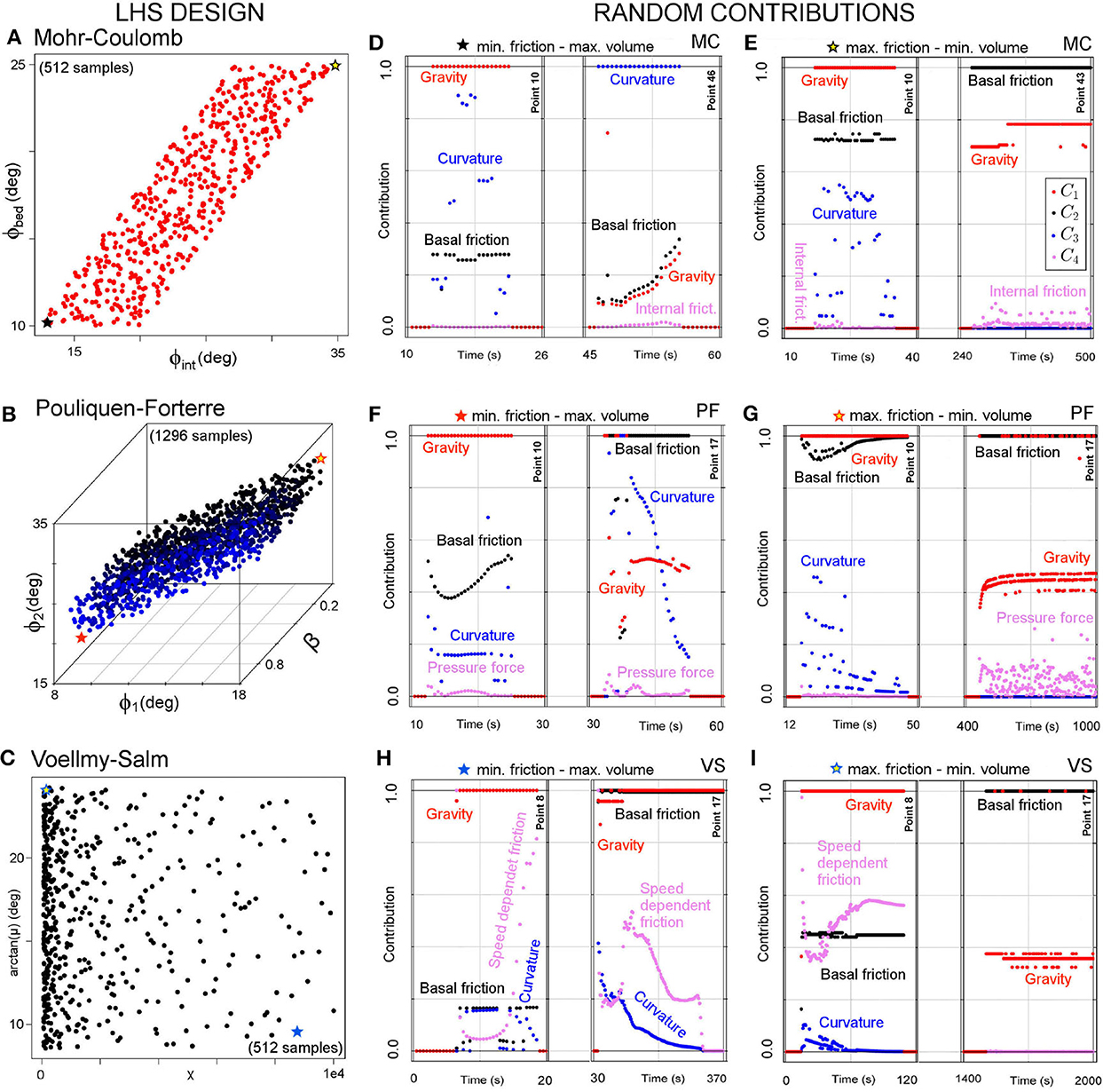
Figure 3. (A–C) Example of Latin Hypercube Sampling design, Volcán de Colima case study. Colored stars mark the values producing the minimum and maximum friction. The parameter values are projected with respect to their volume value. (D–I) Plots of random contributions at specific locations, obtained with (D,E) MC, (F,G) PF, and (H,I) VS model. Each plot includes two graphs. One refers to a proximal location to the initial pile (left), and the other to a more distal location (right). The dominant variable is expressed by the dots on the top line, C_i = 1. Point numbers refer to Figure 5. Different colors correspond to different force terms.

Data is inherently discontinuous due to the mesh modification, and it is reported with colored dots. If the mesh element which contains the considered spatial location changes, then the force term is calculated on a different region and suddenly changes too. This can also affect the dominant variable, and more than one random contribution can incorrectly appear to be at unity at the same time. However, it is evident that the dynamics and its temporal scale is evolving, and that the contributions can reveal a large amount of information about it. We remark that, ∀i, the calculation of 𝔼[C_i] with respect to ${{P}}_M$ removes the effects of data discontinuity, and hence this is a fundamental step in our further analysis. We note that the above choices are easily changed, and if we are interested for instance in the performance of the models for very large or very small flows, a suitable volume range can be chosen and the procedure re-run.

3.3. Observable Outputs

The number of spatial locations is significantly high. We placed 51 points to span the entire inundated area, in search of different flow regimes, as displayed in Figure 1. These locations have an explorative purpose, whereas the six preferred locations will describe distinct flow regimes. We remark that all the distances reported in the following are measured in vertical projection, thus without considering the differences in elevation.

Figure 4 shows the mean flow height, h(L, t), at the 51 spatial locations of interest, according to MC. In Figure 4A, the only location is set on the center of the initial pile. The height profile is bell-shaped, starting from zero and then waning back to zero in ~ 20 s. All the dynamics occur during the first minute. In Figures 4F–J, points are set where the slope reduces, and the flow can channelize, and typically leaves a deposit. The distance from the initial pile is ~ 2 − 3 km.

FIGURE 4

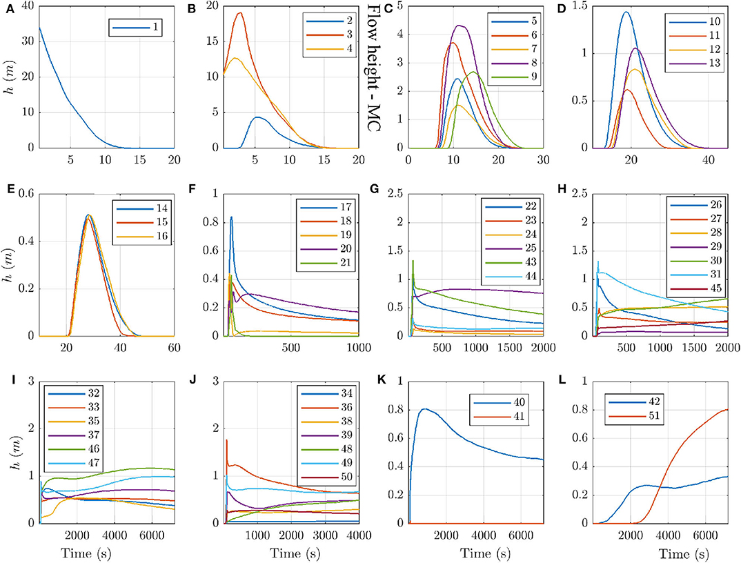
Figure 4. MC model, mean flow height h(L, t) in 51 numbered locations (Figure 1). Plots (A–L) have different scales on either time and space axes.

In general is either observed an initial short-lasting bulge followed by a slow decrease lasting for several minutes and asymptotically tending to a positive height, or a steady increase of material height tending to a positive height. In both cases it is sometimes observed a bimodal profile in the first 5 min. Finally, Figures 4K,L focus on three points set at about the runout distance of the flow, in the most important ravines, at ~ 4 − 5 km from the initial pile.

3.3.1. Flow Height in Six Locations

We select six preferred locations, illustrative of a range of flow regimes. They are [L₈, L₁₀, L₁₇, L₃₉, L₄₃, L₄₆], as displayed in Figure 5. The first two points, L₈ and L₁₀, are both proximal to the initiation pile. Points L₁₇ and L₄₃ are placed where the slope is reducing and the ravines are evident, and L₃₉ and L₄₆ are placed in the channels, further down-slope. In particular, L₈, L₄₃, and L₄₆ are at the western side of the inundated area, whereas L₁₀, L₁₇, and L₃₉ are at the eastern side.

FIGURE 5

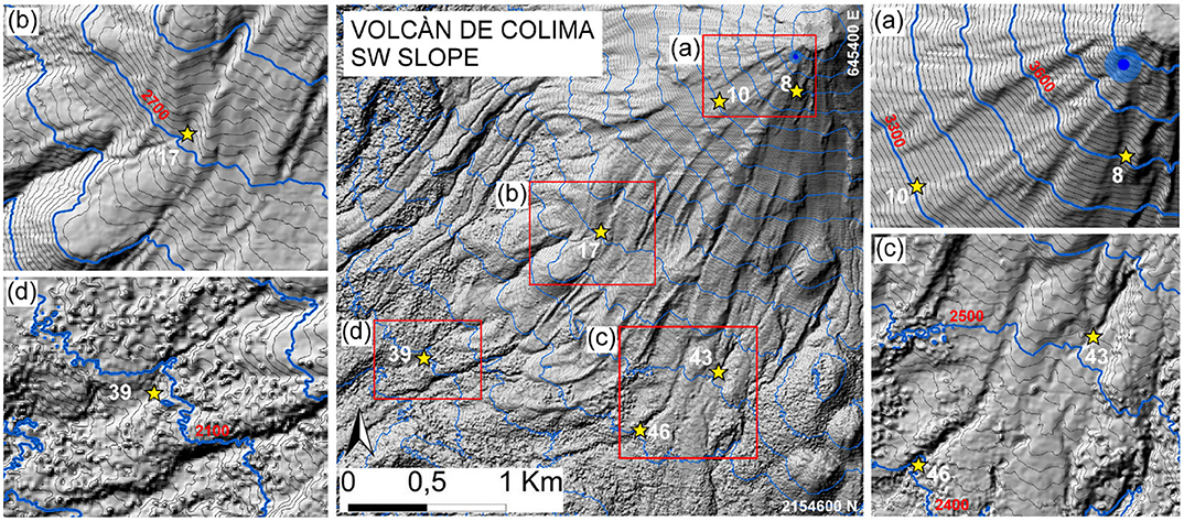
Figure 5. Volcán de Colima (México) overview, including six numbered locations (stars). In panels (a–d) are enlarged the proximal topographic features to those locations. Initial pile is marked by a blue dot. Reported coordinates are in UTM zone 13N. Elevation isolines at every 10m are displayed in black, at every 100m in bold blue. Elevation values in red.

Figure 6 shows the flow height, h(L, t), at the points (L_i)_{i=8,10,17,39,43,46}. Distances from the initial pile are in vertical projection. In Figures 6A,B, we show the flow height in points L₈ and L₁₀, ~ 200m and ~ 500m from the initial pile, respectively. Models MC and PF display similar profiles, positive for less than 15s and bell-shaped. VS requires a significantly longer time to decrease, particularly in point L₁₀, where the average flow height is still positive after ~ 200s. Peak average values in L₈ are 3.4m in PF, 4.3m in MC, 4.7m in VS. Uncertainty is about ±2m, halved on the lower side in MC, and PF. In L₁₀, models MC and PF are very similar, with peak height at 1.4m and uncertainty ±0.5m. Model VS, in contrast, has a maximum height of 1.1m lasting for 50s, and 95^th percentile reaching 3.7m.

FIGURE 6

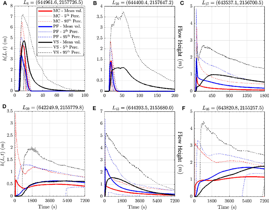
Figure 6. Flow height in six locations. Bold line is mean value, dashed/dotted lines are 5th and 95th percentile bounds. Different models are displayed with different colors. Plots (A–F) show different locations and are at different scale, for simplifying lecture.

In Figures 6C,E, we show the flow height in points L₁₇ and L₄₃, both at ~ 2km from the initial pile. All the models show a fast spike during the first minute, followed by a slow decrease. There is still material after 1800s. VS has a secondary rise peaking at ~ 450s, which is not observed in the other models. This produces higher values for the most of the temporal duration, but similar deposit thickness after more than 1 h. Maximum values are 1m for MC, 2m for PF, and 1.5m for VS, in both locations. The 5^th percentile is zero in all the models, meaning that the parameter range does not always allow the flow to reach these locations. The 95^th percentile is above 5m, except for VS in point L₁₇. In Figures 6D,F, we show the flow height in points L₃₉ and L₄₆, both placed at more than 3km from the initial pile. The three models all show a monotone profile except for MC in point L₃₉, which instead displays an initial spike and a decrease before to rise again. A similar thing is observed in the 95^th percentiles of all the models. It is significant that the 5^th percentile of PF becomes positive after ~ 5, 400s, meaning that almost surely the flow has reached that location. Deposit thickness in point L₃₉ is ~ 0.5m for all the models, whereas in point L₄₆ it is 1.7m in VS, 1.6m in PF, and 1.2m in MC.

We note that VS is temporally stretched compared to the other models, and material arrives later and stays longer in all the sample points. This is a consequence of the speed dependent term reducing flow velocity.

4. Analysis and Discussion

4.1. Contributing Variables Proximal to the Initial Pile

Figure 7 shows the dominance factors (P_i)_i=1,…,4 of the RHS terms modulus, in the three proximal points L₈, L₁₀, and L₁₇, all closer than 1 km to the initial pile. This Figure is modified from Patra et al. (2018a) and its description is reported in this study for the sake of completeness.

FIGURE 7

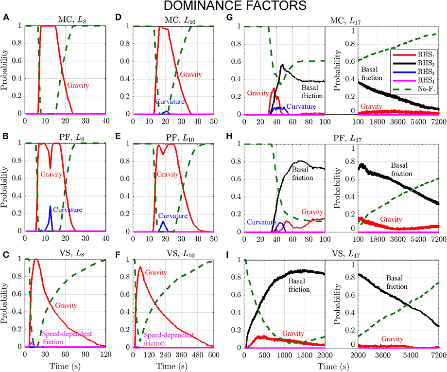
Figure 7. Dominance factors of the forces in three locations in the first km of runout. Different models are plotted separately: (A,D,G) assume MC; (B,E,H) assume PF; (C,F,I) assume VS. Different colors correspond to different force terms. No-flow probability is displayed with a green dashed line.

The plots 7A–C and 7D–F are related to point L₈ and L₁0, respectively. They are significantly similar. The gravitational force RHS₁ is the dominant variable with a very high chance, P₁ > 90%. In MC and PF there is a small probability, P₃ = 5 − −30%, of RHS₃ being the dominant variable for ~ 5s. In VS it is observed a P₄ = 5% chance of RHS₄ being dominant, just for a few seconds. Figures 7G–I concern the relatively more distal point L₁₇. They are split in two sub-frames at different time scale. In all the models, RHS₂ is the most probable dominant variable, and its dominance factor has a bell-shaped profile. In all the models, also RHS₁ has a small chance of being the dominant variable. In MC this chance is more significant, at most P₁ = 30% for ~ 20s, and again P₁ = 2% in [100, 7, 200]s. In PF P₁ = 15% in two peaks, one short lasting at about 55s, and the second extending in [100, 500]s. Also in VS, P₁ = 15% at [300, 500]s. Its profile is unimodal in time and becomes P₁ < 2% after 2, 000s. In MC and PF, RHS₃ has a dominance factor P₃ = 10% at [30, 50]s and [40, 50]s, respectively.

In summary, gravitational force is dominant with a very high chance until the no-flow probability becomes large. In MC and PF curvature related forces can also be dominant for a short time. In VS gravitational force is dominant for a larger time span than in the other models, because of the longer presence of the flow. The speed dependent friction can be dominant with a small probability at the beginning of the dynamics.

Figure 8 shows the corresponding expected contributions 𝔼[C_i]_i=1,…,4. ∀i, C_i is related to the force term RHS_i. The contributions in points L₈ and L₁₀ are shown in Figures 8A–F, respectively. The plots related to the same model are similar. In all the models C₁ is significantly larger than C₂ and C₃, which are almost equivalent in MC and PF, while C₂ > C₃ in VS. C₄ always gives a negligible contribution, except in VS, where it is comparable to C₂. In L₈, following PF, C₃ is bimodal, whereas it is unimodal in MC and VS. This is not observed in L₁₀. In L₈, C₃ is greater than in L₁₀, compared to the other forces. VS always shows a slower decrease of the plots. In plots Figures 8G–I are shown the expected contributions in L₁₇. The plots are split in two sub-frames at different time scale. Initial dynamics is dominated by C₂, except for in MC, and only for a short time, [30, 40]s. In MC there is an initial peak of C₂ which is not observed in the other models. C₃ has a significant size, in MC and PF, and unimodal profile. In PF, after C₃ wanes, at about 60s also C₄ becomes not negligible for ~ 40s. The second part of the temporal domain is characterized by a slow decrease of C₂ > C₁.

FIGURE 8

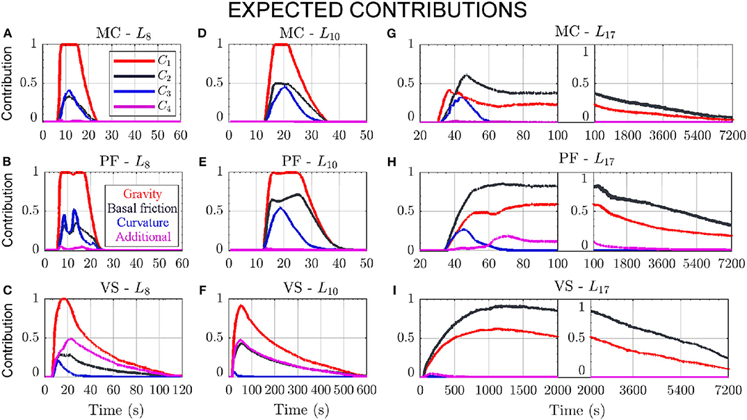
Figure 8. Expected contributions of the forces in three locations in the first km of runout. Different models are plotted separately: (A,D,G) assume MC; (B,E,H) assume PF; (C,F,I) assume VS. Different colors correspond to different force terms.

4.2. Contributing Variables Distal From the Initial Pile

Figure 9 shows the dominance factors (P_i)_i=1,…,4 in the three distal points L₃₉, L₄₃, and L₄₆, all more than 2 km far from the initial pile. Figures 9A–C and L₃₉ are dominated by RHS₁. In all the models P₁ is increasing and P₁ > 90% at the end of the simulation. In MC, P₁ shows a plateau at ~ 40% in [90, 2, 000]s preceded and followed by steep increases, while in the other models it rises gradually. P₂ > 0 after ~ 500 and 3, 600s, respectively, but is never greater than 2%. In MC P₃ ≈ 10% at [50, 70]s. No-flow probability becomes zero in PF and VS, while stops at 20% in MC. Figures 9D–F are related to point L₄₃, and are remarkably complex. In MC, either P₁ and P₂ are ~ 35% in the first 200s. Then, P₂ increases, and RHS₂ becomes the only dominant variable after 3, 600s. The no-flow probability is never below 30%. P₃ = 35% in [40, 60]s. Instead, in PF P₁ > 90% until 3, 600s, and P₂ rises only in the very last amount of time, reaching P₂ = P₁ = 40%. The no-flow probability is very low during the most of the temporal window, rising at 20% only at 7, 200s. Both P₃ and P₄ show short peaks, ~ 10%, at [50, 60]s.

FIGURE 9

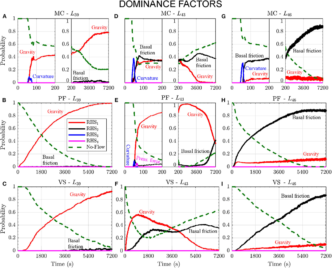
Figure 9. Dominance factors of the forces in three locations after 2 km of runout. Different models are plotted separately: (A,D,G) assume MC; (B,E,H) assume PF; (C,F,I) assume VS. Different colors correspond to different force terms. No-flow probability is displayed with a green dashed line.

In VS the no-flow probability is never below 20%, and the dominance factors are broadly equivalent to MC, although P₁ is the greatest up to 4, 000s, and P₃ ≡ 0. Figures 9G–I are related to point L₄₆ and they are similar to those recorded at point L₁₇, but P₂ > 90% and the no-flow probability decreases to zero in the second half of the simulation. Moreover, in all the models P₁ does not show any initial peak and instead increases slowly, reaching P₁ = 10% after more than 3, 600s.

In summary, only the gravity or the basal friction are dominant with high probability. Some of the points have a deposit at the end with a high chance, some other not, depending on the slope. In general, in MC the no-flow probability tends to be larger than in the other models, because some flow samples stops earlier, or completely leaves the site. Again, curvature can have a small chance to be dominant in MC and PF, particularly when the speed is high. Point L₄₃ deserves a specific discussion. It is not proximal to the initiation, but the no-flow probability is increasing at the end, meaning that all the material tends to leave the site. Moreover, the dominating force can be the gravity or the basal friction depending on the time and the model. In MC and VS both the two forces have similar chances to be dominant for most of the time of the simulation. In PF, only the gravitational force is dominant with a high chance. This is probably because point L₄₃ is situated downhill of a place where a significant amount of material stops.

Figure 10 shows the expected contributions in the distal points. In general, it is worth noting that the remarkable diversity in the dominance factors between the different locations can be the consequence of even a small imbalance between gravity and basal friction. All the plots are dominated by C₁ and C₂, and the remarkable differences observed in the dominance factors depend on which contribution is the greatest. In general these two contributions have similar profiles. Figures 10A–C are related to point L₃₉ and C₁ > C₂. In MC, also is C₃ > 0 for a short time. In MC and PF also C₄ > 0, but it is significantly lower than the previous contributions, almost negligible in MC. Figures 10D–F concern point L₄₃. In MC C₁ < C₂, in PF C₁ > C₂, in VS they C₁ decreases and crosses C₂ at ~ 3, 600s. The two contributions form a plateau in MC, in [90, 200]s. In MC and PF C₃ > 0 for a few seconds, and also C₄ > 0 with an initial spike at ~ 60s. In particular, C₄ reaches ~ 0.05 at point L₄₃, and in Figure 3E we showed that the force contribution can also be at 0.1 in that location, depending on the input values chosen. This means that RHS4 can be about 10% of the dominant force. In PF it shows a long lasting plateau, while becomes negligible in MC. Figures 10G–I are related to point L₄₆. In all the models C₁ < C₂, and these force contributions are monotone increasing. Only in MC C₃ > 0 shortly, and C₄ > 0, but almost negligible.

FIGURE 10

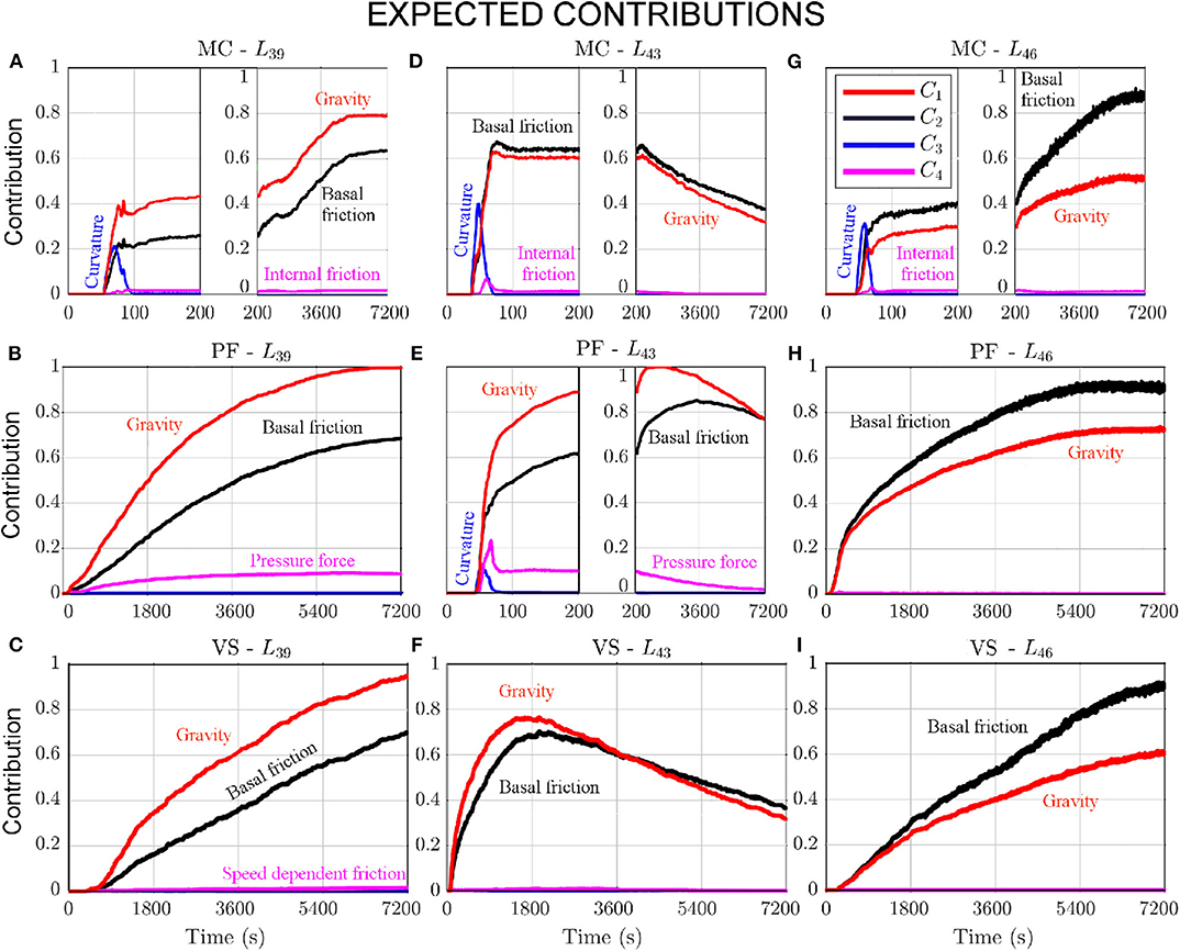
Figure 10. Expected contributions of the forces in three locations after 2 km of runout. Different models are plotted separately: (A,D,G) assume MC; (B,E,H) assume PF; (C,F,I) assume VS. Different colors correspond to different force terms.

4.3. Flow Extent and Spatial Integrals

Figure 11 shows the volumetric average of speed and Froude Number. It also shows the inundated area as a function of time. Spatial averages and inundated area have smoother plots than local measurements, and most of the details observed in local measurements are not easy to discern. In Figure 11A, the speed shows a bell-shaped profile in all the models, but the maximum speed is ~ 60m/s in MC, ~ 50m/s in PF, ~ 20m/s in VS, on average. Uncertainty is ±18m/s in MC, similar, but skewed, in VS, and ±10m/s in PF.

FIGURE 11

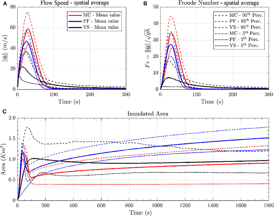
Figure 11. Comparison between spatial averages of (A) flow speed, and (B) Froude Number, in addition to the (C) inundated area, as a function of time. Bold line is mean value, dashed/dotted lines are 5th and 95th percentile bounds. Different models are displayed with different colors. Figure modified from Patra et al. (2018a).

In Figure 11B, the Fr profile is very similar to the speed, but the difference between VS and the other models is accentuated. Maximum values are ~ 50 in MC, ~ 38 in PF, ~ 5 in VS, whereas uncertainty is ±10 in MC, ±7 in PF, and skewed [−5, +10] in VS. In Figure 11C, inundated area has a first peak in MC and PF, both at ~ 1.15km², followed by a decrease to 0.55 and 0.7km², respectively, and then a slower increase up to a flat plateau at 0.9 and 1.5km², respectively. Uncertainty is ~ ±0.2km² in both MC and PF until ~ 100s, and then it increases at ±0.3km² and [−0.5, +0.4]km², respectively. In MC this increase in uncertainty is concentrated at ~ 100s, while it is more gradual in PF. VS has a different profile. The initial peak is only significant in the 95^th percentile values, and occurs later, at ~ 100s. The peak is of ~ 1km² on the average, but up to ~ 1.8km² in the 95^th percentile. The decrease after the peak is very slow and the average inundated area never goes below 0.85km², and eventually reaches back to ~ 1km². Uncertainty is [−0.3, +0.2]km².

4.4. Power Integrals

Figure 12 shows the spatial sum of the powers. The estimates in this section assume ρ = 1, 800kg/m³ as a constant scaling factor. Corresponding plots of the force terms are included in Patra et al. (2018b). The scalar product of force with velocity imposes the bell-shaped profile. In general, gravity term is larger in VS, because a portion of the flow lingers on the higher slopes for a long time. Basal friction has a higher peak in PF compared to the other models, due to the interpolation of the two basal friction angles.

FIGURE 12

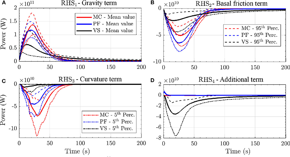
Figure 12. Spatial integrals of the powers. Bold line is mean value, dashed lines are 5th and 95th percentile bounds. Model comparison on the mean value is also displayed. Plots (A–D) show different RHS terms and are at different scale, for simplifying lecture.

In Figure 12A, the power of RHS₁ starts from zero and rises up to 1.4 × 10¹¹ W in MC, 1.2 × 10¹¹ W in PF, 6.5 × 10¹⁰ W in VS. Uncertainty is ±4.0 × 10¹⁰ W in MC, ±3.0 × 10¹⁰ W in PF, [−4.0, 5.0] × 10¹⁰ W in VS. The decrease of gravitational power is related to the slope reduction, and this decrease is more gradual in VS than in the other models. In Figure 12B, the power of RHS₂ is always negative and peaks to −6.5 × 10¹⁰ W in MC, −5.0 × 10¹⁰ W in PF, −2.0 × 10¹⁰ W in VS. In VS this dissipative power is significantly more flat than in the other models. MC and PF show negligible powers after ~ 100s, VS after ~ 200s. Uncertainty is ±2.0 × 10¹⁰ W in MC, ±1.5 × 10¹⁰ W in PF, [−2.0, 1.0] × 10¹⁰ W in VS. In PF, the plot starts from stronger values than in the other models, but it is also the faster to wane. In Figure 12C, the power of RHS₃ shows a negative peak at −7.0 × 10¹⁰ W in MC, −4.5 × 10¹⁰ W in PF, −0.5 × 10¹⁰ W in VS. Uncertainty on the peak value is [−4.5, 3.5] × 10¹⁰ W in MC, [−2.5, 2.0] × 10¹⁰ W in PF, [−1.0, 0.5] × 10¹⁰ W in VS. The three models all show a bell-shaped profile, MC and PF waning to zero at 90s, VS at ~ 30s. In Figure 12D, the power of RHS₄ has a different meaning in the three models. In MC it is the internal friction term, and it only has almost negligible ripple visible in the first second. In PF it is a depth averaged pressure force linked to the thickness gradient, and has a very small effect limited to the first second of simulation, at 0.5 × 10¹⁰ W. It becomes null at ~ 10s. In VS, instead, it is a speed dependent term, and has a very relevant effect. The plot shows a bell-shaped profile, with a peak of −3.5 × 10¹⁰ W, [−2.0, 1.0] × 10¹⁰ W. After that, this dissipative power gradually decreases, and becomes negligible at 200s.

4.5. Example of Model Performance Calculation

Finally, we give an example of model performance evaluation of the couple $(M,{{P}}_M)$ according to a specific observation. In past work (Patra et al., 2005), MC rheology was tuned to match deposits for known block and ash flows, but a priori predictive ability was limited by inability to tune without knowledge of flow character. The new procedure developed in this study enables an enhanced quantification of model performance, i.e., the similarity of the outputs and real data. We remark that the measured performance refers to the couple $(M,{{P}}_M)$, and that different parameter ranges can produce different performances (Tierz et al., 2016; Sandri et al., 2018). This is in contrast with traditional performance analysis based on particular, albeit calibrated, simulations (Charbonnier and Gertisser, 2012).

Our example concerns the Volcán de Colima case study, and in particular we compare the inundated region in our simulations to the deposit of a BAF occurred 16 April 1991 (Rupp, 2004; Saucedo et al., 2004; Rupp et al., 2006). In addition to modeling uncertainty, other uncertainty sources affect this evaluation. For example, our digital elevation map may be different from the exact topography encountered by the real flow, and the inundated region may have been different from the extent of the deposit found in the field. The inundated region is defined as the points in which the maximum flow height H is greater than 10cm. A similar procedure may be applied to any observed variable produced by the models, if specific data become available.

Let ${M}:{C}({ℝ}^2)\to \left[0,1\right]$ be a similarity index defined on the compact subsets of the real plane, i.e., the closed and bounded sets. An equivalent definition can be based on the pseudo-metric $1-{M}$. For example, we define

$\begin{array}{l}{{M}}_1:=\frac{{\displaystyle {\int }_{{ℝ}^2}}{1}_D(\text{x})d\text{x}}{{\displaystyle {\int }_{{ℝ}^2}}{1}_{S\cup D}(\text{x})d\text{x}},{{M}}_2:=\frac{{\displaystyle {\int }_{{ℝ}^2}}{1}_{S\cap D}(\text{x})d\text{x}}{{\displaystyle {\int }_{{ℝ}^2}}{1}_D(\text{x})d\text{x}},\\ {J}:={{M}}_1·{{M}}_2,\end{array}$

where S ⊂ ℝ² is the inundated region, and D ⊂ ℝ² is the recorded deposit.

In particular, ${{M}}_1$ is the area of the deposit over the area of the union of inundated region and deposit, ${{M}}_2$ is the area of the intersection of inundated region and deposit over the area of the deposit, ${J}$ is the product of the previous, also called Jaccard Index (Jaccard, 1901). Figure 13 shows the probability distribution of the similarity indices, according to the uniform probability ${{P}}_M$ on the parameter ranges defined in this study. Different metrics can produce different performance estimates, for example MC inundates most of the deposit, but overestimates the inundated region, while VS relatively reduces the inundated region outside of the deposit boundary, but also leaves several not-inundated spots inside it.

FIGURE 13

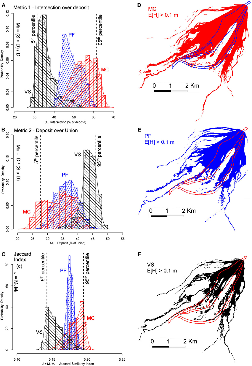
Figure 13. Volcán de Colima. Pdf of the similarity index of inundated regions and a real BAF deposit. Panel (A) is based on ${{M}}_I$, (B) on ${{M}}_U$, (C) on ${J}$. The models are MC (red), PF (blue), VS (black). Data histograms are displayed in the background. Global 5th and 95th percentile values are indicated with dashed lines. Plots (D–F) display the average inundated region {x : E[H(x)] > 10cm}. The boundary of the real deposit is marked with a colored line.

Let g :[a, b] → [0, 1] be a score function defined over the percentile range of the similarity index. The global 5^th and 95^th percentile values [a, b] are defined assuming to select the model randomly with equal chance, and are also shown in Figures 13A–C.

Then the performance score G_g of model $(M,{{P}}_M)$ is defined as:

$\begin{array}{l}{G}_g(M,{{P}}_M)={\displaystyle {\int }_{\left[a,b\right]}}g(x)d{f}_M(x),\end{array}$

where f_M is the pdf related to the model. Possible score functions include a step function at the global median, a linear or quadratic function, a sigmoid function. Table 1 shows alternative performance scores, according to changing similarity indices and score functions.

TABLE 1

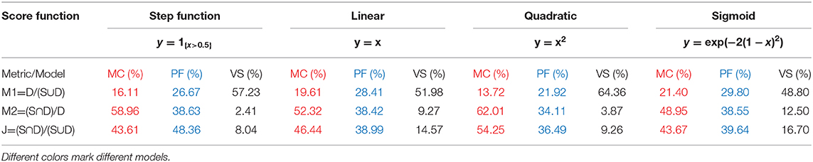
Table 1. Performance scores as a function of model, performance metric, and score function.

5. Conclusions

In this study, we have described a statistically driven method for investigating the constituents of complex models. We implemented three different models composed of different assumptions about rheology in geophysical mass flows to illustrate the approach. The data objectively shows the performance of the models over many possible flow regimes and topographies. The analysis of contributing variables illustrates the impact of several modeling assumptions. Understanding which assumptions dominate, and by how much, is a key step toward the construction of more efficient models for desired inputs. Such model composition is the subject of ongoing and future work, with the purpose of bypassing the search for a unique best model, and going beyond a simple mixture of alternative models.

In summary, our new method enabled us to break down the effects of the different physical assumptions in the dynamics, providing an improved understanding of what characterizes each model. The procedure was applied to the Digital Elevation Map (DEM) of the SW slope of Volcán de Colima (MX). In particular, we presented:

• A short review of the assumptions characterizing three commonly used rheologies of Mohr-Coulomb, Poliquenne-Forterre, Voellmy-Salm. This included a qualitative list of such assumptions, and a breaking down of the different terms in the differential equations.

• A new statistical framework, processing the mean and the uncertainty range of either observable or contributing variables in the simulations. The new concepts of dominance factors and expected contributions enabled a simplified description of the local dynamics. These quantities were analyzed at selected sites, and spatial integrals were calculated, which illustrate the characteristics of the entire flow.

• The contribution coefficients C_i and dominance factors P_i introduced here allow us to quantify and compare in a probabilistic framework the effect of modeling assumptions based on the full range of flows explored using statistically rigorous ensemble computations.

• A final discussion, explaining all the observed features in the results in light of the known physical assumptions of the models, and the evolving flow regime in space and time. This included an example of the model performance estimation method, which depends on the metric and the cost function adopted.

Our analysis uncovered the following main features of the different geophysical models used in the example analysis:

• Compared to the standard MC model, the lack of internal friction in the PF model produces an accentuated lateral spread. The spread is increased by the uninhibited internal pressure force, which briefly pushes the flow ahead and laterally during the initial collapse. That force can also have some minor effects in the accumulation of the final deposit. The interpolation between the smaller bed friction angle ϕ₁ and the larger value ϕ₂ in the PF model suddenly stops the flow if it is thin compared to its speed. This mechanism suppresses large peaks in flow speed.

• In VS, the speed-dependent friction has a great effect in reducing lateral spread and producing channelized flow even where there are otherwise minor ridges and adverse slopes in the topography. The flow tends to be significantly slower and more stretched out in the downslope direction. The effects of different formulations of the curvature term have less impact than do the effects of lower basal friction and speed.

• In our case study the internal friction term in the MC model has a relatively small impact on the dynamics of the flow. Neglecting the term will be a meaningful choice if workload reduction is required in future analyses.

Furthermore, we can make the following statements about the technique in terms of its use on models in general:

• It gives information not only on which forces in the equations of motion are dominating the flow, but also shows where these forces are greatest and gives insight into why they locally peak and vary, and into the impacts of the dominating forces on the model flow outputs,

• It provides a new, quantitative technique to evaluate the most important forces or phenomena acting in a particular model domain, which can supplement, provide insight and guidance into, and generate quantitative information for, the more typical methods used in force analysis of intuition and Similarity Theory.

Additional research concerning other case studies, and different parameter ranges, might reveal other flow regimes, and hence differences in the consequences of the modeling assumptions under new circumstances.

Data Availability Statement

The datasets generated for this study are available on request to the corresponding author.

Author's Note

An extended version of this manuscript has been released at https://arxiv.org/abs/1805.12104 (Patra et al., 2018b). In particular, Patra et al. (2018b) includes a further analysis of the additional case study of a small scale flow on inclined plane and flat runway, as well as additional details on the latin hypercubes based on orthogonal arrays, and supplementary datasets including estimates of local Froude Numbers and spatial integrals of force terms.

Author Contributions

AP and AB conceived the main conceptual ideas. AB and AA-S implemented and performed the simulations and optimization calculations. AB and AP interpreted the computational results and wrote the paper. All authors discussed the results, commented on the manuscript, provided critical feedback, and gave final approval for publication.

Funding

We would like to acknowledge the support of NSF awards 1521855, 1621853, and 1339765.

Conflict of Interest

The authors declare that the research was conducted in the absence of any commercial or financial relationships that could be construed as a potential conflict of interest.

Footnotes

1. ^Available online at: vhub.org.

2. ^We thank the University at Buffalo Center for Computing Research.

References

Aghakhani, H., Dalbey, K., Salac, D., and Patra, A. K. (2016). Heuristic and Eulerian interface capturing approaches for shallow water type flow and application to granular flows. Comput. Methods Appl. Mech. Eng. 304, 243–264. doi: 10.1016/j.cma.2016.02.021

CrossRef Full Text | Google Scholar

Ai, M., Kong, X., and Li, K. (2016). A general theory for orthogonal array based Latin hypercube sampling. Stat. Sin. 26, 761–777. doi: 10.5705/ss.202015.0029

CrossRef Full Text | Google Scholar

Bartelt, P., and McArdell, B. (2009). Granulometric investigations of snow avalanches. J. Glaciol. 55, 829–833. doi: 10.3189/002214309790152384

CrossRef Full Text | Google Scholar

Bartelt, P., Salm, B., and Gruber, U. (1999). Calculating dense-snow avalanche runout using a Voellmy-fluid model with active/passive longitudinal straining. J. Glaciol. 45, 242–254. doi: 10.1017/S002214300000174X

CrossRef Full Text | Google Scholar

Bayarri, M. J., Berger, J. O., Calder, E. S., Dalbey, K., Lunagomez, S., Patra, A. K., et al. (2009). Using statistical and computer models to quantify volcanic hazards. Technometrics 51, 402–413. doi: 10.1198/TECH.2009.08018

CrossRef Full Text | Google Scholar

Bayarri, M. J., Berger, J. O., Calder, E. S., Patra, A. K., Pitman, E. B., Spiller, E. T., et al. (2015). Probabilistic quantification of hazards: a methodology using small ensembles of physics-based simulations and statistical surrogates. Int. J. Uncertain. Quant. 5, 297–325. doi: 10.1615/Int.J.UncertaintyQuantification.2015011451

CrossRef Full Text | Google Scholar

Bevilacqua, A., Patra, A. K., Bursik, M. I., Pitman, E. B., Macías, J. L., Saucedo, R., et al. (2019). Probabilistic forecasting of plausible debris flows from Nevado de colima (Mexico) using data from the atenquique debris flow, 1955. Nat. Hazards Earth Syst. Sci. 19, 791–820. doi: 10.5194/nhess-19-791-2019

CrossRef Full Text | Google Scholar

Bongard, J., and Lipson, H. (2007). Automated reverse engineering of nonlinear dynamical systems. Proc. Natl. Acad. Sci. U.S.A. 104, 9943–9948. doi: 10.1073/pnas.0609476104

PubMed Abstract | CrossRef Full Text | Google Scholar

Bursik, M., Patra, A., Pitman, E., Nichita, C., Macias, J., Saucedo, R., et al. (2005). Advances in studies of dense volcanic granular flows. Rep. Prog. Phys. 68:271. doi: 10.1088/0034-4885/68/2/R01

CrossRef Full Text | Google Scholar

Capra, L., Gavilanes-Ruiz, J. C., Bonasia, R., Saucedo-Giron, R., and Sulpizio, R. (2015). Re-assessing volcanic hazard zonation of Volcán de Colima, Mexico. Nat. Hazards 76, 41–61. doi: 10.1007/s11069-014-1480-1

CrossRef Full Text | Google Scholar

Capra, L., Macís, J., Cortés, A., Dávila, N., Saucedo, R., Osorio-Ocampo, S., et al. (2016). Preliminary report on the July 10-11, 2015 eruption at Volcán de Colima: pyroclastic density currents with exceptional runouts and volume. J. Volcanol. Geotherm. Res. 310(Suppl. C), 39–49. doi: 10.1016/j.jvolgeores.2015.11.022

CrossRef Full Text | Google Scholar

Capra, L., Manea, V. C., Manea, M., and Norini, G. (2011). The importance of digital elevation model resolution on granular flow simulations: a test case for Colima volcano using TITAN2D computational routine. Nat. Hazards 59, 665–680. doi: 10.1007/s11069-011-9788-6

CrossRef Full Text | Google Scholar

Charbonnier, S., Germa, A., Connor, C., Gertisser, R., Preece, K., Komorowski, J.-C., et al. (2013). Evaluation of the impact of the 2010 pyroclastic density currents at Merapi volcano from high-resolution satellite imagery, field investigations and numerical simulations. J. Volcanol. Geotherm. Res. 261(Suppl. C), 295–315. doi: 10.1016/j.jvolgeores.2012.12.021

CrossRef Full Text | Google Scholar

Charbonnier, S., and Gertisser, R. (2012). Evaluation of geophysical mass flow models using the 2006 block-and-ash flows of Merapi volcano, Java, Indonesia: towards a short-term hazard assessment tool. J. Volcanol. Geotherm. Res. 231–232:87–108. doi: 10.1016/j.jvolgeores.2012.02.015

CrossRef Full Text | Google Scholar

Charbonnier, S. J., and Gertisser, R. (2009). Numerical simulations of block-and-ash flows using the Titan2D flow model: examples from the 2006 eruption of Merapi Volcano, Java, Indonesia. Bull. Volcanol. 71, 953–959. doi: 10.1007/s00445-009-0299-1

CrossRef Full Text | Google Scholar

Christen, M., Kowalski, J., and Bartelt, P. (2010). RAMMS: Numerical simulation of dense snow avalanches in three-dimensional terrain. Cold Regions Sci. Technol. 63, 1–14. doi: 10.1016/j.coldregions.2010.04.005

CrossRef Full Text | Google Scholar

Dade, W. B., and Huppert, H. E. (1998). Long-runout rockfalls. Geology 26, 803–806. doi: 10.1130/0091-7613(1998)026<0803:LRR>2.3.CO;2

CrossRef Full Text | Google Scholar

Dalbey, K., Patra, A. K., Pitman, E. B., Bursik, M. I., and Sheridan, M. F. (2008). Input uncertainty propagation methods and hazard mapping of geophysical mass flows. J. Geophys. Res. Solid Earth 113, 1–16. doi: 10.1029/2006JB004471

CrossRef Full Text | Google Scholar

Dalbey, K. R. (2009). Predictive simulation and model based hazard maps (Ph.D. thesis). University at Buffalo, Buffalo, NY, United States.

Google Scholar

Davila, N., Capra, L., Gavilanes-Ruiz, J., Varley, N., Norini, G., and Vazquez, A. G. (2007). Recent lahars at Volcán de Colima (Mexico): drainage variation and spectral classification. J. Volcanol. Geotherm. Res. 165, 127–141. doi: 10.1016/j.jvolgeores.2007.05.016

CrossRef Full Text | Google Scholar

de' Michieli Vitturi, M., Esposti Ongaro, T., Lari, G., and Aravena, A. (2019). Imex_sflow2d 1.0: a depth-averaged numerical flow model for pyroclastic avalanches. Geosci. Model Dev. 12, 581–595. doi: 10.5194/gmd-12-581-2019

CrossRef Full Text | Google Scholar

Denlinger, R. P., and Iverson, R. M. (2001). Flow of variably fluidized granular masses across three-dimensional terrain: 2. Numerical predictions and experimental tests. J. Geophys. Res. 106, 553–566. doi: 10.1029/2000JB900330

CrossRef Full Text | Google Scholar

Denlinger, R. P., and Iverson, R. M. (2004). Granular avalanches across irregular three-dimensional terrain: 1. Theory and computation. J. Geophys. Res. 109:F01014. doi: 10.1029/2003JF000085

CrossRef Full Text | Google Scholar

Drucker, D. C., and Prager, W. (1952). Soil mechanics and plastic analysis for limit design. Q. Appl. Math. 10, 157–165. doi: 10.1090/qam/48291

CrossRef Full Text | Google Scholar

Farrell, K., Tinsley, J., and Faghihi, D. (2015). A Bayesian framework for adaptive selection, calibration, and validation of coarse-grained models of atomistic systems. J. Comput. Phys. 295, 189–208. doi: 10.1016/j.jcp.2015.03.071

CrossRef Full Text | Google Scholar

Fischer, J., Kowalski, J., and Pudasaini, S. P. (2012). Topographic curvature effects in applied avalanche modeling. Cold Regions Sci. Technol. 74–75:21–30. doi: 10.1016/j.coldregions.2012.01.005

CrossRef Full Text | Google Scholar

Forterre, Y., and Pouliquen, O. (2002). Stability analysis of rapid granular chute flows: formation of longitudinal vortices. J. Fluid Mech. 467, 361–387. doi: 10.1017/S0022112002001581

CrossRef Full Text | Google Scholar

Forterre, Y., and Pouliquen, O. (2003). Long-surface-wave instability in dense granular flows. J. Fluid Mech. 486, 21–50. doi: 10.1017/S0022112003004555

CrossRef Full Text | Google Scholar

González, M. B., Ramírez, J. J., and Navarro, C. (2002). Summary of the historical eruptive activity of Volcán De Colima, Mexico 1519-2000. J. Volcanol. Geotherm. Res. 117, 21–46. doi: 10.1016/S0377-0273(02)00233-0

CrossRef Full Text | Google Scholar

Gray, J. M. N. T., Wieland, M., and Hutter, K. (1999). Gravity-driven free surface flow of granular avalanches over complex basal topography. Proc. R. Soc. Lond. Ser. A Math. Phys. Eng. Sci. 455, 1841–1874. doi: 10.1098/rspa.1999.0383

CrossRef Full Text | Google Scholar

Gruber, U., and Bartelt, P. (2007). Snow avalanche hazard modelling of large areas using shallow water numerical models and GIS. Environ. Modell. Softw. 22, 1472–1481. doi: 10.1016/j.envsoft.2007.01.001

CrossRef Full Text | Google Scholar

Higdon, D., Kennedy, M., Cavendish, J. C., Cafeo, J. A., and Ryne, R. D. (2004). Combining field data and computer simulations for calibration and prediction. SIAM J. Sci. Comput. 26, 448–466. doi: 10.1137/S1064827503426693

CrossRef Full Text | Google Scholar

Hyman, D., and Bursik, M. (2018). Deformation of volcanic materials by pore pressurization: analog experiments with simplified geometry. Bull. Volcanol. 80:19. doi: 10.1007/s00445-018-1201-9

CrossRef Full Text | Google Scholar

Hyman, D. M., Bevilacqua, A., and Bursik, M. I. (2019). Statistical theory of probabilistic hazard maps: a probability distribution for the hazard boundary location. Nat. Hazards Earth Syst. Sci. 19, 1347–1363. doi: 10.5194/nhess-19-1347-2019

CrossRef Full Text | Google Scholar

Iverson, R. M. (1997). The physics of debris flows. Rev. Geophys. 35, 245–296. doi: 10.1029/97RG00426

CrossRef Full Text | Google Scholar

Iverson, R. M., and Denlinger, R. P. (2001). Flow of variably fluidized granular masses across three-dimensional terrain: 1. Coulomb mixture theory. J. Geophys. Res. 106:537. doi: 10.1029/2000JB900329

CrossRef Full Text | Google Scholar

Iverson, R. M., and George, D. L. (2014). A depth-averaged debris-flow model that includes the effects of evolving dilatancy. I. Physical basis. Proc. R. Soc. Lond. A Math. Phys. Eng. Sci. 470:2170. doi: 10.1098/rspa.2013.0819

CrossRef Full Text | Google Scholar

Iverson, R. M., Logan, M., and Denlinger, R. P. (2004). Granular avalanches across irregular three-dimensional terrain: 2. Experimental tests. J. Geophys. Res. Earth Surface 109:F01015. doi: 10.1029/2003JF000084

CrossRef Full Text | Google Scholar

Jaccard, P. (1901). Distribution de la flore alpine dans le bassin des Dranses et dans quelques régions voisines. Bull. Soc. Vaudoise Sci. Nat. 37, 241–272.

Google Scholar

Kelfoun, K. (2011). Suitability of simple rheological laws for the numerical simulation of dense pyroclastic flows and long-runout volcanic avalanches. J. Geophys. Res. 116:B08209. doi: 10.1029/2010JB007622

CrossRef Full Text | Google Scholar

Kelfoun, K., and Druitt, T. H. (2005). Numerical modeling of the emplacement of Socompa rock avalanche, Chile. J. Geophys. Res. Solid Earth 110:B12. doi: 10.1029/2005JB003758

CrossRef Full Text | Google Scholar

Kelfoun, K., Samaniego, P., Palacios, P., and Barba, D. (2009). Testing the suitability of frictional behaviour for pyroclastic flow simulation by comparison with a well-constrained eruption at Tungurahua volcano (Ecuador). Bull. Volcanol. 71, 1057–1075. doi: 10.1007/s00445-009-0286-6

CrossRef Full Text | Google Scholar

Kennedy, M. C., and O'Hagan, A. (2011). Bayesian calibration of computer models. J. R. Stat. Soc. Ser. B Stat. Methodol. 63, 425–464. doi: 10.1111/1467-9868.00294

CrossRef Full Text

Kern, M., Bartelt, P., Sovilla, B., and Buser, O. (2009). Measured shear rates in large dry and wet snow avalanches. J. Glaciol. 55, 327–338. doi: 10.3189/002214309788608714

CrossRef Full Text | Google Scholar

la Cruz-Reyna, S. D. (1993). Random patterns of occurrence of explosive eruptions at Colima Volcano, Mexico. J. Volcanol. Geotherm. Res. 55, 51–68. doi: 10.1016/0377-0273(93)90089-A

CrossRef Full Text | Google Scholar

Macías, J., Capra, L., Arce, J., Espíndola, J., García-Palomo, A., and Sheridan, M. (2008). Hazard map of El Chichón volcano, Chiapas, México: constraints posed by eruptive history and computer simulations. J. Volcanol. Geotherm. Res. 175, 444–458. doi: 10.1016/j.jvolgeores.2008.02.023

CrossRef Full Text | Google Scholar

Macorps, E., Charbonnier, S. J., Varley, N. R., Capra, L., Atlas, Z., and Cabré, J. (2018). Stratigraphy, sedimentology and inferred flow dynamics from the July 2015 block-and-ash flow deposits at Volcán de Colima, Mexico. J. Volcanol. Geotherm. Res. 349, 99–116. doi: 10.1016/j.jvolgeores.2017.09.025

CrossRef Full Text | Google Scholar

Martin Del Pozzo, A. M., Sheridan, M. F., Barrera, M., Hubp, J. L., and Selem, L. V. (1995). Potential hazards from Colima Volcano, Mexico. Geofisica Int. 34, 363–376.

McKay, M. D., Beckman, R. J., and Conover, W. J. (1979). A comparison of three methods for selecting values of input variables in the analysis of output from a computer code. Technometrics 21, 239–245. doi: 10.1080/00401706.1979.10489755

CrossRef Full Text | Google Scholar

Norini, G., De Beni, E., Andronico, D., Polacci, M., Burton, M., and Zucca, F. (2009). The 16 November 2006 flank collapse of the south-east crater at Mount Etna, Italy: study of the deposit and hazard assessment. J. Geophys. Res. Solid Earth 114:B02204. doi: 10.1029/2008JB005779

CrossRef Full Text | Google Scholar

Ogburn, S. E., Berger, J., Calder, E. S., Lopes, D., Patra, A., Pitman, E. B., et al. (2016). Pooling strength amongst limited datasets using hierarchical Bayesian analysis, with application to pyroclastic density current mobility metrics. Stat. Volcanol. 2, 1–26. doi: 10.5038/2163-338X.2.1

CrossRef Full Text | Google Scholar

Owen, A. B. (1992a). A central limit theorem for Latin hypercube sampling. J. R. Stat. Soc. 54, 541–551. doi: 10.1111/j.2517-6161.1992.tb01895.x

CrossRef Full Text | Google Scholar

Owen, A. B. (1992b). Orthogonal arrays for computer experiments, integration and visualization. Stat. Sin. 2, 439–452.

Google Scholar

Patra, A., Bevilacqua, A., and Akhavan-Safaei, A. (2018a). “Analyzing complex models using data and statistics,” in Computational Science-ICCS 2018, eds Y. Shi, H. Fu, Y. Tian, V. V. Krzhizhanovskaya, M. H. Lees, J. Dongarra, and P. M. A. Sloot (Cham: Springer International Publishing), 724–736. doi: 10.1007/978-3-319-93701-4_57

PubMed Abstract | CrossRef Full Text | Google Scholar

Patra, A., Bevilacqua, A., Akhavan-Safaei, A., Pitman, E., Bursik, M., and Hyman, D. (2018b). Comparative analysis of the structures and outcomes of geophysical flow models and modeling assumptions using uncertainty quantification. arXiv [preprint] arXiv:1805.12104. Available online at: https://arxiv.org/abs/1805.12104

Google Scholar

Patra, A., Nichita, C., Bauer, A., Pitman, E., Bursik, M., and Sheridan, M. (2006). Parallel adaptive discontinuous Galerkin approximation for thin layer avalanche modeling. Comput. Geosci. 32, 912–926. doi: 10.1016/j.cageo.2005.10.023

CrossRef Full Text | Google Scholar

Patra, A. K., Bauer, A. C., Nichita, C. C., Pitman, E. B., Sheridan, M. F., Bursik, M., et al. (2005). Parallel adaptive numerical simulation of dry avalanches over natural terrain. J. Volcanol. Geotherm. Res. 139, 1–21. doi: 10.1016/j.jvolgeores.2004.06.014

CrossRef Full Text | Google Scholar

Pirulli, M., Bristeau, M.-O., Mangeney, A., and Scavia, C. (2007). The effect of the earth pressure coefficients on the runout of granular material. Environ. Modell. Softw. 22, 1437–1454. doi: 10.1016/j.envsoft.2006.06.006

CrossRef Full Text | Google Scholar

Pitman, E. B., and Le, L. (2005). A two-fluid model for avalanche and debris flows. Philos. Trans. Ser. A Math. Phys. Eng. Sci. 363, 1573–1601. doi: 10.1098/rsta.2005.1596

PubMed Abstract | CrossRef Full Text | Google Scholar

Pitman, E. B., Nichita, C. C., Patra, A., Bauer, A., Sheridan, M., and Bursik, M. (2003). Computing granular avalanches and landslides. Phys. Fluids 15:3638. doi: 10.1063/1.1614253

CrossRef Full Text | Google Scholar

Popper, K. R. (1959). The Logic of Scientific Discovery. London; New York, NY: Routledge. doi: 10.1063/1.3060577

PubMed Abstract | CrossRef Full Text | Google Scholar

Pouliquen, O. (1999). Scaling laws in granular flows down rough inclined planes. Phys. Fluids 11, 542–548. doi: 10.1063/1.869928

PubMed Abstract | CrossRef Full Text | Google Scholar

Pouliquen, O., and Forterre, Y. (2002). Friction law for dense granular flows: application to the motion of a mass down a rough inclined plane. J. Fluid Mech. 453, 133–151. doi: 10.1017/S0022112001006796

CrossRef Full Text | Google Scholar

Procter, J. N., Cronin, S. J., Platz, T., Patra, A., Dalbey, K., Sheridan, M., et al. (2010). Mapping block-and-ash flow hazards based on Titan 2D simulations: a case study from Mt. Taranaki, NZ. Nat. Hazards 53, 483–501. doi: 10.1007/s11069-009-9440-x

CrossRef Full Text | Google Scholar

Ranjan, P., and Spencer, N. (2014). Space-filling Latin hypercube designs based on randomization restrictions in factorial experiments. Stat. Probabil. Lett. 94(Suppl. C):239–247. doi: 10.1016/j.spl.2014.07.032

CrossRef Full Text | Google Scholar

Rankine, W. J. M. (1857). On the stability of loose earth. Philos. Trans. R. Soc. Lond. 147, 9–27. doi: 10.1098/rstl.1857.0003

CrossRef Full Text | Google Scholar

Reyes-Dávila, G. A., Arámbula-Mendoza, R., Espinasa-Perena, R., Pankhurst, M. J., Navarro-Ochoa, C., Savov, I., et al. (2016). Volcan de Colima dome collapse of July, 2015 and associated pyroclastic density currents. J. Volcanol. Geotherm. Res. 320(Suppl. C), 100–106. doi: 10.1016/j.jvolgeores.2016.04.015

CrossRef Full Text | Google Scholar

Rupp, B. (2004). An analysis of granular flows over natural terrain (Master's thesis). University at Buffalo, Buffalo, NY, United States.

Rupp, B., Bursik, M., Namikawa, L., Webb, A., Patra, A. K., Saucedo, R., et al. (2006). Computational modeling of the 1991 block and ash fows at Colima Volcano, México. Geol. Soc. Am. Spcl. Pap. 402, 223–237. doi: 10.1130/2006.2402(11)

CrossRef Full Text | Google Scholar

Rutarindwa, R., Spiller, E. T., Bevilacqua, A., Bursik, M. I., and Patra, A. K. (2019). Dynamic probabilistic hazard mapping in the long valley volcanic region ca: integrating vent opening maps and statistical surrogates of physical models of pyroclastic density currents. J. Geophys. Res. Solid Earth 124, 9600–9621. doi: 10.1029/2019JB017352

CrossRef Full Text | Google Scholar

Salm, B. (1993). Flow, flow transition and runout distances of flowing avalanches. Ann. Glaciol. 18, 221–226. doi: 10.1017/S0260305500011551

CrossRef Full Text | Google Scholar

Salm, B., Burkard, A., and Gubler, H. (1990). Berechnung von Fliesslawinen: eine Anleitung für Praktiker mit Beispielen¨. Mitteilungen des Eidgenössische Institutes für Schnee- und Lawinenforschung, 47.

Saltelli, A., Annoni, P., Azzini, I., Campolongo, F., Ratto, M., and Tarantola, S. (2010). Variance based sensitivity analysis of model output. Design and estimator for the total sensitivity index. Comput. Phys. Commun. 181, 259–270. doi: 10.1016/j.cpc.2009.09.018

CrossRef Full Text | Google Scholar

Sandri, L., Tierz, P., Costa, A., and Marzocchi, W. (2018). Probabilistic hazard from pyroclastic density currents in the Neapolitan area (southern Italy). J. Geophys. Res. Solid Earth 123, 3474–3500. doi: 10.1002/2017JB014890

CrossRef Full Text | Google Scholar

Sarocchi, D., Sulpizio, R., Macías, J., and Saucedo, R. (2011). The 17 July 1999 block-and-ash flow (BAF) at Colima Volcano: New insights on volcanic granular flows from textural analysis. J. Volcanol. Geotherm. Res. 204, 40–56. doi: 10.1016/j.jvolgeores.2011.04.013

CrossRef Full Text | Google Scholar

Saucedo, R., Macías, J., Bursik, M., Mora, J., Gavilanes, J., and Cortes, A. (2002). Emplacement of pyroclastic flows during the 1998-1999 eruption of Volcán de Colima, México. J. Volcanol. Geotherm. Res. 117, 129–153. doi: 10.1016/S0377-0273(02)00241-X

CrossRef Full Text | Google Scholar

Saucedo, R., Macías, J., Gavilanes, J., Arce, J., Komorowski, J., Gardner, J., and Valdez-Moreno, G. (2010). Eyewitness, stratigraphy, chemistry, and eruptive dynamics of the 1913 Plinian eruption of Volcán de Colima, México. J. Volcanol. Geotherm. Res. 191, 149–166. doi: 10.1016/j.jvolgeores.2010.01.011

CrossRef Full Text | Google Scholar

Saucedo, R., Macías, J., Sheridan, M., Bursik, M., and Komorowski, J. (2005). Modeling of pyroclastic flows of Colima Volcano, Mexico: implications for hazard assessment. J. Volcanol. Geotherm. Res. 139, 103–115. doi: 10.1016/j.jvolgeores.2004.06.019

CrossRef Full Text | Google Scholar

Saucedo, R., Macías, J. L., and Bursik, M. (2004). Pyroclastic flow deposits of the 1991 eruption of Volcán de Colima, México. Bull. Volcanol. 66, 291–306. doi: 10.1007/s00445-003-0311-0

CrossRef Full Text | Google Scholar

Savage, S. B., and Hutter, K. (1989). The motion of a finite mass of granular material down a rough incline. J. Fluid Mech. 199:177. doi: 10.1017/S0022112089000340

CrossRef Full Text | Google Scholar

Sheridan, M., Stinton, A., Patra, A., Pitman, E., Bauer, A., and Nichita, C. (2005). Evaluating Titan2D mass-flow model using the 1963 Little Tahoma Peak avalanches, Mount Rainier, Washington. J. Volcanol. Geotherm. Res. 139, 89–102. doi: 10.1016/j.jvolgeores.2004.06.011

CrossRef Full Text | Google Scholar

Sheridan, M. F., and Macías, J. L. (1995). Estimation of risk probability for gravity-driven pyroclastic flows at Volcan Colima, Mexico. J. Volcanol. Geotherm. Res. 66, 251–256. doi: 10.1016/0377-0273(94)00058-O

CrossRef Full Text | Google Scholar

Sheridan, M. F., Patra, A. K., Dalbey, K., and Hubbard, B. (2010). “Probabilistic digital hazard maps for avalanches and massive pyroclastic flows using TITAN2D,” in Stratigraphy and Geology of Volcanic Areas, eds G. Groppelli and L. Viereck-Goette (Boulder, CO: Geological Society of America), 281. doi: 10.1130/2010.2464(14)

CrossRef Full Text | Google Scholar

Simakov, N. A., Jones-Ivey, R. L., Akhavan-Safaei, A., Aghakhani, H., Jones, M. D., and Patra, A. K. (2019). “Modernizing TITAN2D, a parallel AMR geophysical flow code to support multiple rheologies and extendability,” in International Conference on High Performance Computing (Frankfurt: Springer), 101–112. doi: 10.1007/978-3-030-34356-9_10

CrossRef Full Text | Google Scholar

Spiller, E. T., Bayarri, M. J., Berger, J. O., Calder, E. S., Patra, A. K., Pitman, E. B., et al. (2014). Automating emulator construction for geophysical hazard maps. SIAM/ASA J. Uncertain. Quant. 2, 126–152. doi: 10.1137/120899285

CrossRef Full Text | Google Scholar

Stefanescu, E. R., Bursik, M., Cordoba, G., Dalbey, K., Jones, M. D., Patra, A. K., et al. (2012a). Digital elevation model uncertainty and hazard analysis using a geophysical flow model. Proc. R. Soc. Lond. A Math. Phys. Eng. Sci. 468, 1543–1563. doi: 10.1098/rspa.2011.0711

CrossRef Full Text | Google Scholar

Stefanescu, E. R., Bursik, M., and Patra, A. K. (2012b). Effect of digital elevation model on Mohr-Coulomb geophysical flow model output. Nat. Hazards 62, 635–656. doi: 10.1007/s11069-012-0103-y

CrossRef Full Text | Google Scholar

Stein, M. (1987). Large sample properties of simulations using Latin hypercube sampling. Technometrics 29, 143–151. doi: 10.1080/00401706.1987.10488205

CrossRef Full Text | Google Scholar

Sulpizio, R., Capra, L., Sarocchi, D., Saucedo, R., Gavilanes-Ruiz, J., and Varley, N. (2010). Predicting the block-and-ash flow inundation areas at Volcán de Colima (Colima, Mexico) based on the present day (February 2010) status. J. Volcanol. Geotherm. Res. 193, 49–66. doi: 10.1016/j.jvolgeores.2010.03.007

CrossRef Full Text | Google Scholar

Tang, B. (1993). Orthogonal array-based Latin hypercubes. J. Am. Stat. Assoc. 88, 1392–1397. doi: 10.1080/01621459.1993.10476423

CrossRef Full Text | Google Scholar

Tierz, P., Sandri, L., Costa, A., Zaccarelli, L., Di Vito, M. A., Sulpizio, R., and Marzocchi, W. (2016). Suitability of energy cone for probabilistic volcanic hazard assessment: validation tests at Somma-Vesuvius and Campi Flegrei (Italy). Bull. Volcanol. 78:79. doi: 10.1007/s00445-016-1073-9

CrossRef Full Text | Google Scholar

Tierz, P., Stefanescu, E. R., Sandri, L., Sulpizio, R., Valentine, G. A., Marzocchi, W., et al. (2018). Towards quantitative volcanic risk of pyroclastic density currents: probabilistic hazard curves and maps around somma-vesuvius (Italy). J. Geophys. Res. Solid Earth 123, 6299–6317. doi: 10.1029/2017JB015383

CrossRef Full Text | Google Scholar

Voellmy, A. (1955). Über die Zerstörungskraft von Lawinen. Schweiz Bauzeitung 73, 159–165, 212-217, 246-249, 280-285.

Google Scholar

Weirs, V. G., Kamm, J. R., Swiler, L. P., Tarantola, S., Ratto, M., Adams, B. M., et al. (2012). Sensitivity analysis techniques applied to a system of hyperbolic conservation laws. Reliabil. Eng. Syst. Saf. 107, 157–170. doi: 10.1016/j.ress.2011.12.008

CrossRef Full Text | Google Scholar

Wolpert, R., Ogburn, S., and Calder, E. (2016). The longevity of lava dome eruptions. J. Geophys. Res. Solid Earth 121, 676–686. 2015JB012435. doi: 10.1002/2015JB012435

CrossRef Full Text | Google Scholar

Yu, B., Dalbey, K., Webb, A., Bursik, M., Patra, A. K., Pitman, E. B., et al. (2009). Numerical issues in computing inundation areas over natural terrains using Savage-Hutter theory. Nat. Hazards 50, 249–267. doi: 10.1007/s11069-008-9336-1

CrossRef Full Text | Google Scholar

Zobin, V., Arámbula, R., Bretón, M., Reyes, G., Plascencia, I., Navarro, C., et al. (2015). Dynamics of the January 2013-June 2014 explosive-effusive episode in the eruption of Volcán de Colima, México: insights from seismic and video monitoring. Bull. Volcanol. 77:31. doi: 10.1007/s00445-015-0917-z

CrossRef Full Text | Google Scholar

Zobin, V., Luhr, J., Taran, Y., Bretón, M., Cortés, A., De La Cruz-Reyna, S., et al. (2002). Overview of the 1997-2000 activity of Volcán de Colima, México. J. Volcanol. Geotherm. Res. 117, 1–19. doi: 10.1016/S0377-0273(02)00232-9

CrossRef Full Text | Google Scholar