Discrete Boltzmann Numerical Simulation of Simplified Urban Flooding Configurations Caused by Dam Break

1. Introduction

Flooding is considered one of the most significant hazards society is facing. Huge losses in terms of human lives, damages to buildings, houses, and civil infrastructures are caused every year by hurricanes and flooding. Moreover, the impact of flooding in the future is expected to become increasingly important due to deforestation and depopulation of rural zones (Sanders and Schubert, 2019).

Urban flooding are particularly fearsome events, considering that more than half of the world's population lives in urban areas and that the urban population is continuously increasing (Song et al., 2019). The prediction of expected consequences of urban flooding as well as the design and the adoption of mitigation measures is a crucial issue that nowadays takes advantages of numerical simulations.

The main mathematical model for flood simulation is based on the two-dimensional Shallow Water Equations (SWE), which is obtained by averaging mass and momentum balance equations along the vertical direction under the classical assumption of hydrostatic pressure distribution (Valiani and Begnudelli, 2006). In the last decades, great attention has been paid to the development of numerical solvers for the SWE (Toro and Garcia-Navarro, 2007; Toro, 2009). The latter tackle directly the SWE by means of the finite volumes discretization and have reached a sufficient level of complexity so that they are able to account for crucial issues such as to cite just a few, the treatment of topography source terms (Duran and Marche, 2014; Hou et al., 2018), the use of unstructured grids (Zhao et al., 2019), and the evolution of wet-dry fronts (Ferrari et al., 2019).

An alternative option is represented by the Smoothed Particle Hydrodynamics (SPH) formulation of the SWE (Chang et al., 2018). The latter give rise to strongly non-linear equations whose numerical treatment needs particular care. Moreover, the numerical algorithms of SPH-based methods are intrinsically non-local, thus implying typically a high computational burden.

Solution methods for the SWE have also been developed in the Lattice Boltzmann Equation (LBE) framework (Zhou, 2004); these methods take advantage of the simplicity and versatility of the stream and collide LBE algorithm (Succi, 2001). The LBE proposes a mesoscopic representation of the flows based on the concept of the probability density function associated to a fluid particle traveling along a given direction with a given particle velocity (Succi, 2001). The finite set of particle velocities is defined in such a way that a symmetric regular spatial lattice is generated (Succi, 2001). Macroscopic quantities, such as vertically averaged velocity and water depth in shallow water flows, are calculated as statistical moments of the probability density functions (Zhou, 2004). However, no matter how appealing the application of the LBE to shallow water flows may be, the LBE is limited to the simulation of subcritical flows unless an ad hoc-defined lattice is adopted instead of the usual one, as in Hedjripour et al. (2016), where only one-dimensional transcritical shallow water flows have been considered. This is an unacceptable limitation, as the simulation of flooding problems cannot rule out the occurrence of transcritical flows. This fact addressed the research toward the use of multispeed particle velocity sets together with a finite difference discretization of the Boltzmann equation. The resulting model, the multispeed Discrete Boltzmann Equation (DBE), is able to deal with transcritical flows, both 1D and 2D, preserving the linearity of the LBE numerical algorithm (La Rocca et al., 2015). The DBE has been also successfully applied to the investigation of the dynamics of two-phase (La Rocca et al., 2018) and polydisperse (La Rocca et al., 2019) shallow granular flows.

The aim of this paper is to assess the ability of the DBE in simulating dam-break flows impacting on obstacles as a preliminary step for the simulation of urban flooding events on real topography. Indeed dam-break flows impacting on obstacles can be considered as simplified models of urban flooding, and the scientific literature abounds with experiments and numerical simulations of dam-break flows impacting on obstacles. In this paper, the experimental and numerical dam-break flows of Kleefsman et al. (2005), Soares-Frazão and Zech (2007), and Soares-Frazão and Zech (2008) are considered as benchmarks. In Kleefsman et al. (2005) and Soares-Frazão and Zech (2007), the dam-break flow interacts with an isolated obstacle, while in Soares-Frazão and Zech (2008) the dam-break flow interacts with an idealized city, which realized by means of a regular array of parallelepipeds.

In these works, water depth and velocity are measured at given measurement points and/or are numerically calculated by means of previously validated finite volume-based numerical solvers either applied to the SWE (Soares-Frazão and Zech, 2007, 2008), or to the Navier-Stokes equations (Kleefsman et al., 2005). A comparison between numerical results obtained solving the SWE by means of the DBE and reference results is encouraging and proves the ability of the DBE as a simulation tool of dam break flows interacting with obstacles.

The structure of the paper is as follows: first, the mathematical model is briefly presented; second, the considered benchmarks are described; third, results are reported and commented on; and fourth, conclusions are drawn.

2. The Mathematical Model

The SWE, obtained by averaging mass and momentum balance equations along the vertical direction under the classical assumption of hydrostatic pressure distribution (Valiani and Begnudelli, 2006), assume the following form:

$\begin{array}{l}\frac{\partial h}{\partial t}+\frac{\partial Uh}{\partial x}+\frac{\partial Vh}{\partial y}=0\\ \frac{\partial Uh}{\partial t}+\frac{\partial }{\partial x}\left(U^{2}h+g\frac{h^2}{2}\right)+\frac{\partial }{\partial y}(UVh)=\frac{\partial }{\partial x}{\left(g\frac{h^2}{2}\right)|}_{\eta }\\ -g\frac{n_m^2}{h^{1/3}}U\sqrt{U^2+V^2}\\ \frac{\partial Vh}{\partial t}+\frac{\partial }{\partial x}(UVh)+\frac{\partial }{\partial y}\left(V^{2}h+g\frac{h^2}{2}\right)={\frac{\partial }{\partial y}\left(g\frac{h^2}{2}\right)|}_{\eta }\\ -g\frac{n_m^2}{h^{1/3}}V\sqrt{U^2+V^2}& (1)\end{array}$

where h is the water depth and U, V the vertically averaged velocity components along the horizontal directions x, y respectively. n_m is the Manning friction coefficient.

The first term at right hand side of the second and third Equation (1) accounts for the bottom slope and is calculated as in Valiani and Begnudelli (2006), i.e., taking as a constant the free surface elevation η, defined as the following: η = z_f+h, being z_f the bottom elevation. This formulation of the bottom slope term ensures the correct balance between flux gradients and source terms (Valiani and Begnudelli, 2006). The free surface η is considered instantaneously and locally constant: i.e., it is constant within the computational cell during the time step.

The DBE is given by (La Rocca et al., 2015):

$\begin{array}{ll}\frac{\partial f_k}{\partial t}+c_{xk}\frac{\partial f_k}{\partial x}+c_{yk}\frac{\partial f_k}{\partial y}=\frac{f_k^{eq}-f_k}{{\tau }^{*}}+2\frac{F_x^e{c}_{xk}+F_y^e{c}_{yk}}{\sum _k(c_{xk}^2+c_{yk}^2)}& (2)\end{array}$

where f_k is the probability density function relative to the kth particle velocity, whose cartesian components along x, y are respectively c_xk, c_yk. The particle velocity set as the kth equilibrium probability density function $f_k^{eq}$ is defined in La Rocca et al. (2015) and reported concisely in the Appendix for the reader's convenience. τ^* is the dimensional relaxation time, $F_x^e,F_y^e$ are the cartesian components of the external forces acting on the flow. In this case, they are defined by the following:

$\begin{array}{l}{F}_x^e=\frac{\partial }{\partial x}{\left(g\frac{h^2}{2}\right)|}_{\eta }-g\frac{n_m^2}{h^{1/3}}U\sqrt{U^2+V^2}\\ F_y^e=\frac{\partial }{\partial y}{\left(g\frac{h^2}{2}\right)|}_{\eta }-g\frac{n_m^2}{h^{1/3}}V\sqrt{U^2+V^2}& (3)\end{array}$

The DBE (2) is equivalent to the SWE (1) in the sense that the water depth h and the unit discharges Uh, Vh, obtained as the zero and first order moments of f_k

$\begin{array}{ll}\begin{array}{c}h={\displaystyle \sum _k}{f}_k\\ Uh={\displaystyle \sum _k}{c}_{xk}{f}_k\\ Vh={\displaystyle \sum _k}{c}_{yk}{f}_k\end{array}& (4)\end{array}$

coincide with the water depth h and the unit discharges Uh, Vh that are obtained by solving the SWE (1) provided that the ratio Fr/Re of the Froude and the Reynolds number of the flow is small (La Rocca et al., 2015).

It is worth observing that the DBE (2) that consists of a set of uncoupled, linear advection equations with constant advection velocity; this is the most appealing aspect of the DBE, when compared with the highly non-linear SWE, and it is an advantage per se. Indeed, the numerical solution of the DBE can be tackled by means of computational methods that are rather simple in comparison with those needed to treat the complex non-linearities of the SWE. Such an advantage may involve a gain of efficiency, whose quantification is, however, very difficult, as it depends on a variety of factors, such as e.g., the level of coding optimization and parallelization, the performance of the processors, etc., and this is beyond the scope of this work.

3. Experimental Dam Break Flows

3.1. Computational Details

The DBE (2) is discretized by means of an explicit first order approximation of the time derivative and a first order upwind approximation of the space derivative (La Rocca et al., 2015). Details of the numerical discretization, which is rather standard, can be found in Fletcher (2012) and are not reported here for the sake of concision. Boundary conditions are imposed on the macroscopic variables (water depth and vertically averaged velocity); then, the probability density functions at equilibrium are calculated and the values assigned as boundary values to the probability density functions (Ubertini et al., 2003). Stability is ensured by setting the order of magnitude of the Courant number C (C = U_max × Δt/Δs) to O(10⁻¹), U_max, Δt, and Δs being the highest celerity of flow perturbations, the time step, and the space step, respectively. The adopted numerical method introduces numerical viscosity proportional to Δs, whose effect decreases by increasing the number of computational grid points. Finally, the value of the dimensionless relaxation time τ, defined as τ = τ^*/Δt has been chosen in the range 0.5 < τ < 0.6.

3.2. Dam-Break Flow Impacting on an Isolated Obstacle-I

This case has been considered in Kleefsman et al. (2005) and many subsequent works, as it is widely used as benchmark to validate free-surface software (Kees et al., 2011). The reader can refer to Kees et al. (2011) for a detailed description of the experimental setup. The experimental configuration, realized at the Maritime Research Institute Netherlands (MARIN) in a tank (3.22 × 1.00 × 1.00 m), consists of a column of water at rest (height 0.55 m, length 0.58 m, and width 1 m) separated by a sliding gate from the rest of the tank where the water level is zero. By lifting the gate, the water column collapses under the action of gravity and impinges on a fixed parallelepiped (0.40 × 0.16 × 0.16 m) placed at 2.40 m from the right end of the tank, giving rise to a complex dam-break flow traveling back and forth within the tank. The Manning coefficient is estimated to the following: $n_m\approx 0.01s/m^{1/3}$. The experimental setup is equipped with four heights (H₁, H₂, H₃, and H₄) and four pressure probes (P₁−P₄) (Kees et al., 2011).

In Figure 1, the plots of the DBE numerical profiles of the free surface at t = 0.4s and t = 0.56 are compared to the corresponding experimental profiles of Kleefsman et al. (2005). At t = 0.4s the flow has almost reached the obstacle, while at t = 0.56 the impact has occurred, and the formation of a water splash with a height of around 0.4 m is evident both in the experiment and in the numerical simulation. The position of the height (H₁, H₂, H₃, and H₄) and pressure (P₃) probes is also reported in Figure 1.

FIGURE 1

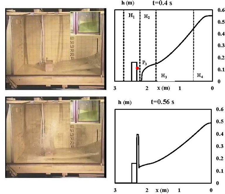
Figure 1. Test case I. Experimental and numerical free surface profiles at t = 0.4s and t = 0.56. Right: numerical free surface profiles. Top right panel shows gauges positioning along the centreline. Vertical dashed lines: positions of the height probes H₁, H₂, H₃, and H₄; dot on the obstacle: position of the P3 pressure probe. Left: experimental profiles of Kleefsman et al. (2005).

In Figure 2, the time history of the water height at probes H₁, H₂, H₃, and H₄ is plotted. Dots represent the experimental results obtained at MARIN, while the solid line represents the DBE numerical results. The latter are those obtained with the finest grid (800 × 280). The space step Δs is equal to 4 × 10⁻³m, while the order of magnitude of the time step Δt is O(10⁻⁴)s. The general agreement is fairly good. The main discrepancy between experimental and numerical results is evident for the probe H2, where the DBE results overestimate the peak of water height due to the impact of the flow on the obstacle, and this is attributed to the fact that the shallow water model does not describe correctly the strong vertical dynamics involved during impact; the duration is, however, very short in comparison to the duration of the considered experiment. However, it is interesting to observe that the instant of impact of the flow on the obstacle (t ≈ 0.5s) is correctly predicted by the DBE numerical results. The experimental and numerical time history of the pressure measured by the probe P₃ is shown in Figure 3. In the framework of the shallow water equations, the numerical pressure is calculated assuming a hydrostatic pressure distribution: p = ρg(h−z), z being the elevation of the pressure gauge from the bottom of the tank. The experimental pressure shows an isolated peak, due to the sudden impact of the water against the obstacle, which is a typical dynamic feature and of course cannot be reproduced by the numerical hydrostatic pressure distribution. However, as time goes by, dynamic effect loose importance and the hydrostatic pressure distribution becomes a fair representation of the pressure field.

FIGURE 2

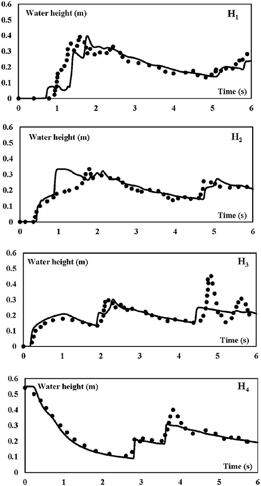
Figure 2. Test case I. Time history of the water height at probes H₁, H₂, H₃, and H₄. Solid lines: DBE numerical results. Dots: Experimental results.

FIGURE 3

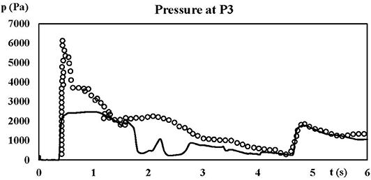
Figure 3. Test case I. Time history of the pressure at probe P₃. Solid line: DBE numerical results. Dots: Experimental results.

3.3. Dam-Break Flow Impacting on an Isolated Obstacle-II

This case has been considered in Soares-Frazão and Zech (2007), where the reader can find a detailed description of the experimental setup. The experiments have been realized in a tank 36 m long, 3.6 m wide, with a trapezoidal cross section. A gate (width 1 m), placed 7.70 m from the left end of the tank, separates the reservoir from the part of the tank representing a valley with an isolated building. The latter is a parallelepipedal obstacle, with a 0.8 × 0.4 m base area. The 0.8 m long side is inclined at an angle of 64° with respect to the y axis (Soares-Frazão and Zech, 2007). The water level is set to 0.4 m and 0.02 m within the reservoir and the rest of the tank, respectively.

Finally, the Manning coefficient is set to $n_m\approx 0.01s/m^{1/3}$ as in Soares-Frazão and Zech (2007). Water height and velocity measurements have been performed at several points (Soares-Frazão and Zech, 2007). Velocity values are measured at 0.036 m from the bottom and cannot be compared with the DBE numerical vertically averaged velocity, as the flow presents intense re-circulation zones with high values of the vertical velocity component.

In Figure 4 are plotted the time histories of the free surface at measurement points G₁, G₃, G₄, and G₆. Solid lines represent experimental values, while dotted and dashed lines represent the DBE numerical values obtained with a coarse (600 × 67) and a fine (1500 × 165) grid, respectively. The difference between the DBE numerical results obtained with the two grids is not meaningful, mainly at measurement point G₆. The differences with the experimental results observed at measurement points G₁, G₃, G₄, and G₆ are ascribed to the fact that there the vertical motions are not negligible and that the shallow water model loses consistency. Nevertheless, the DBE numerical results grab the main features of the flow, and the general agreement with experiments can be considered fairly good. The DBE numerical results are in satisfying agreement with the numerical results of Noël et al. (2003), reported in Soares-Frazão and Zech (2007) and obtained by directly integrating the SWE. This fact is depicted in Figure 5 where the snapshots of the free surface at t = 1s, t = 3s, and t = 10s reproduce the same flow features observed in the numerical calculation of Noël et al. (2003).

FIGURE 4

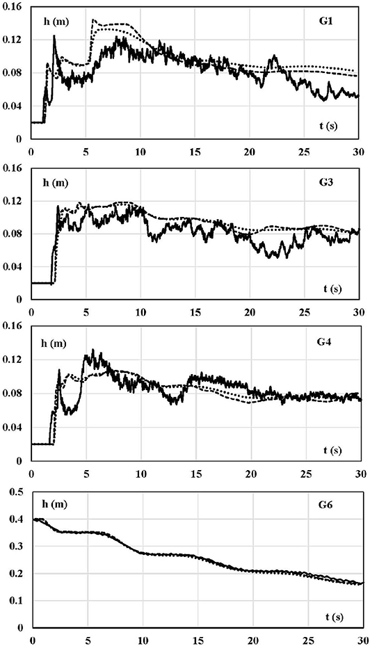
Figure 4. Test case II. Experimental and numerical free surface time histories. Solid line: experimental measurements from Soares-Frazão and Zech (2007). Dotted line: DBE numerical results obtained with the coarse grid. Dashed line: DBE numerical results obtained with the fine grid.

FIGURE 5

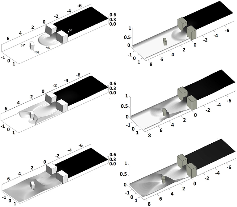
Figure 5. Test case II. Free surface at t = 1s, t = 3s, t = 10s. Left: DBE results; right: numerical results from Soares-Frazão and Zech (2007) ; top-left panel shows gauges positioning̱.

3.4. Dam-Break Flow Impacting on an Idealized City

This case is reported in Soares-Frazão and Zech (2008), where the experimental setup is described with great detail, and has been performed with the same experimental setup tank used in Soares-Frazão and Zech (2007). The idealized city has been realized by means of 25 impervious wooden blocks of 0.30 m × 0.30 m, representing buildings, separated by streets 0.10 m wide and arranged in a regular array of 5 × 5. According to Soares-Frazão and Zech (2008), the ratio of the street to building width is realistic despite the strong simplification of the representation of the city.

A gate (width 1 m), placed 7.70 m from the left end of the tank, separates the reservoir from the part of the tank containing the idealized city. The water level is set to 0.4 m and 0.011 m within the reservoir and the rest of the tank, respectively. Finally, the Manning coefficient is set to $n_m\approx 0.01s/m^{1/3}$ as in Soares-Frazão and Zech (2008). Water height has been measured by means of several resistive level gauges, placed along straight lines along the streets of the city, while velocity has been measured both on the free surface, by means of a digital-imaging technique, and close to the bottom by means of an acoustic doppler velocimeter (ADV) (Soares-Frazão and Zech, 2008).

In Figure 6, the DBE numerical results and the experimental and numerical results of Soares-Frazão and Zech (2008) relative to the free surface profile at 4s, 5s, and 6s are shown. The free surface profile is plotted along the third longitudinal street. The agreement is satisfying. Minor discrepancies at t = 5s can be attributed to numerical oscillations in the central part of the obstacles' array. In Figure 7, the DBE numerical Froude number profile at t = 4s along the third longitudinal street, as indicated by the sketch, is shown. The high values attained by the Froude number allow to state that the DBE is a robust tool to investigate super- and transcritical flows. It is worth observing the fairly good agreement among the DBE numerical and experimental velocity values and that the position of the main hydraulic jump (x ~ 4.3 ÷ 4.4 m), shown in Figure 6, matches with the sudden change from Fr > 1 to Fr < 1 of the Froude number shown in Figure 7. Finally, in Figure 8 the computed water depth in the neighborhood of the city area is shown at t = 5s, t = 10s, respectively. The complex features of the flow comply with those shown in Soares-Frazão and Zech (2008).

FIGURE 6

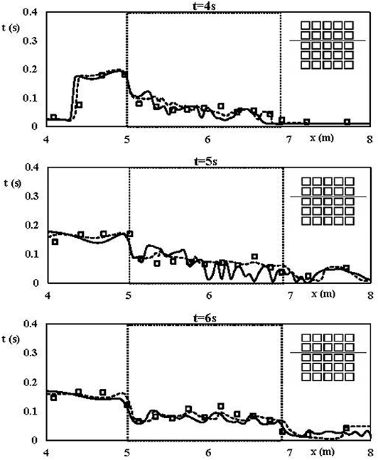
Figure 6. Test case III. Experimental dam break flow through an idealized city of Soares-Frazão and Zech (2008). Free surface profile at 4, 5, and 6s along the third longitudinal street, as indicated by the sketch. Solid line: DBE numerical results. Dashed line: Soares-Frazão and Zech (2008) numerical results. Dots: Soares-Frazão and Zech (2008) experimental values. Dotted box: area occupied by the buildings.

FIGURE 7

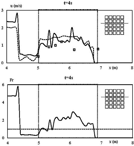
Figure 7. Test case III. Experimental dam break flow through an idealized city of Soares-Frazão and Zech (2008). Bottom: Froude number profile at 4s along the third longitudinal street, as indicated by the sketch. Solid line: DBE numerical results. Dotted box: area occupied by the buildings. Top: u velocity profile at 4s along the third longitudinal street, as indicated by the sketch. Solid line: DBE numerical results. Dashed line: shallow water numerical results of Soares-Frazão and Zech (2008). Dots: experimental results of Soares-Frazão and Zech (2008).

FIGURE 8

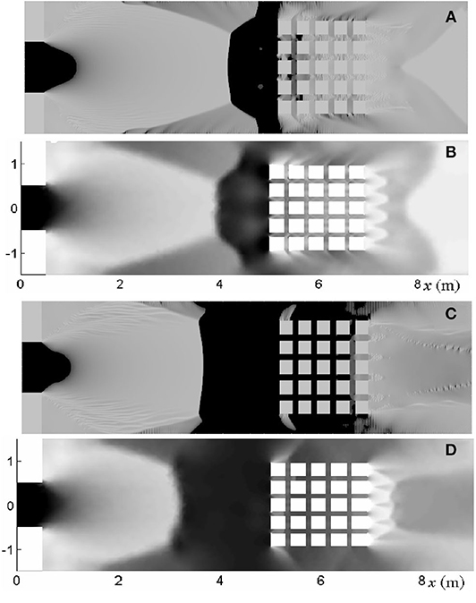
Figure 8. Test case III. Computed water depth map. Darker color for larger depth values. Top panels (A,B): t = 5s; bottom panels (C,D): t = 10s. Panels (A,C): DBE numerical results. Panels (B,D) are numerical values from Soares-Frazão and Zech (2008).

In particular, at t = 5s (Figures 8A,B), the flow between the gate and the city is mainly supercritical; it forms a sort of hat-like shaped subcritical zone downstream of a hydraulic jump which front is placed at x_H = 3.95 m along the centerline of the tank. From the edges of the subcritical zone, at x_E = 4m, y_EN = 0.7 m, and x_E = 4m, y_ES = −0.7 m, two symmetrical oblique waves detach and end at the wall of the tank (Figures 8A,B). Points x_H, x_E, y_EN, and y_ES coincide in Figures 8A,B. Within the longitudinal street of the city the flow is mainly supercritical, as in Soares-Frazão and Zech (2008). Finally, the wake zone immediately downstream of the city, where a triangular wave is observable, is qualitatively similar to that observed in Soares-Frazão and Zech (2008).

At t = 10s (Figures 8C,D), the structure of the flow is similar to that observed at t = 5s. The subrictical zone is almost rectangular, the front being located at x_H = 3.4 m along the centerline of the tank. The two symmetrical oblique waves detach from the points x_E = 3.3m, y_EN = 1.0 m and x_E = 3.3m, y_ES = −1.0 m. Points x_H, x_E, y_EN, and y_ES coincide in Figures 8C,D. Within the longitudinal street of the city the flow is mainly subcritical, as in Soares-Frazão and Zech (2008), while it becomes supercritical in the wake zone immediately downstream of the city.

4. Concluding Remarks

The multispeed Discrete Boltzmann Equation (DBE) is a method recently developed to simulate transcritical shallow water flows, and the main advantage is the simplicity of the mathematical model: a set of linear, uncoupled, purely advective equations. In this paper, the DBE has been assessed as solution method for the Shallow Water Equation (SWE) when dam-break flows impacting on obstacles are considered. These flows are strongly unsteady and present frequent sub-supercritical and super-subcritical (hydraulic jumps) transitions.

The consideration of dam-break flows impacting on obstacles is important as they represent simplified models of urban flooding, thus constituting a benchmark for numerical methods, thanks to the wide variety of reference numerical and experimental data published in literature.

In this paper, three dam-break flows impacting obstacles have been considered: two on an isolated obstacle and one on an idealized city that has realized by means of a regular array of parallelepipeds.

The experimental configurations were realized within tanks with a smooth, though sloping, bottom. The latter has been treated in order to account for the correct balance between flux gradients and source terms.

The comparison between DBE and reference results (both numerical and experimental) shows that the DBE can be considered as a reliable solution method for dam break flows impacting on obstacles, even in the presence of complex flow configurations, such as e.g., the case of the idealized city. Discrepancies between DBE and reference results can be attributed both to the use of coarse grids and to the accuracy of the numerical method and to the occurrence of violent vertical motions, which undermine the consistency of the shallow water model. It is worth observing that, for what regards the specific performance of the proposed models in urban areas, there are no restrictions for the DBE on the attainable grid resolutions. Any grid convergence rate can be achieved by just adopting a higher order numerical scheme. Future works will be addressed to the consideration of realistic topography as well as to the implementation of more efficient numerical methods, such as e.g., the finite volume method with unstructured, adaptive grids.

Data Availability Statement

The datasets generated for this study are available on request to the corresponding author.

Author Contributions

ML has formulated the Discrete Boltzmann Equation. PP performed the numerical simulations. SM analyzed the results and prepared graphics. All the authors have discussed together about the outcomes and their interpretation. All authors contributed to the article and approved the submitted version.

Funding

The authors acknowledged funding from the Italian Ministry of Education, University and Research (MIUR), in the frame of the Departments of Excellence Initiative 2018–2022, attributed to the Department of Engineering of Roma Tre University.

Conflict of Interest

The authors declare that the research was conducted in the absence of any commercial or financial relationships that could be construed as a potential conflict of interest.

Acknowledgments

Valuable discussions with Dr. A. Montessori are kindly acknowledged.

References

Chang, K. H., Sheu, T. W. H., and Chang, T. J. (2018). A 1D–2D coupled SPH-SWE model applied to open channel flow simulations in complicated geometries. Adv. Water Resour. 115, 185–197. doi: 10.1016/j.advwatres.2018.03.009

CrossRef Full Text | Google Scholar

Duran, A., and Marche, F. (2014). Recent advances on the discontinuous Galerkin method for shallow water equations with topography source terms. Comput. Fluids 101, 88–104. doi: 10.1016/j.compfluid.2014.05.031

CrossRef Full Text | Google Scholar

Ferrari, A., Viero, D. P., Vacondio, R., Defina, A., and Mignosa, P. (2019). Flood inundation modeling in urbanized areas: a mesh-independent porosity approach with anisotropic friction. Adv. Water Resour. 125, 98–113. doi: 10.1016/j.advwatres.2019.01.010

CrossRef Full Text | Google Scholar

Fletcher, C. A. J. (2012). Computational Techniques for Fluid Dynamics 1: Fundamentals and General Techniques. Berlin; Heidelberg; New York, NY: Springer Science & Business Media.

PubMed Abstract | Google Scholar

Hedjripour, A. H., Callaghan, D. P., and Baldock, T. E. (2016). Generalized transformation of the lattice Boltzmann method for shallow water flows. J. Hydraul. Res. 54, 371–388. doi: 10.1080/00221686.2016.1168881

CrossRef Full Text | Google Scholar

Hou, J., Wang, R., Liang, Q., Li, Z., Huang, M. S., and Hinkelmann, R. (2018). Efficient surface water flow simulation on static Cartesian grid with local refinement according to key topographic features. Comput. Fluids 176, 117–134. doi: 10.1016/j.compfluid.2018.03.024

CrossRef Full Text | Google Scholar

Kees, C. E., Akkerman, I., Farthing, M. W., and Bazilevs, Y. (2011). A conservative level set method suitable for variable-order approximations and unstructured meshes. J. Comput. Phys. 230, 4536–4558. doi: 10.1016/j.jcp.2011.02.030

CrossRef Full Text | Google Scholar

Kleefsman, K. M. T., Fekken, G., Veldman, A. E. P., Iwanowski, B., and Buchner, B. (2005). A volume-of-fluid based simulation method for wave impact problems. J. Comput. Phys. 206, 363–393. doi: 10.1016/j.jcp.2004.12.007

PubMed Abstract | CrossRef Full Text | Google Scholar

La Rocca, M., Montessori, A., Prestininzi, P., and Elango, L. (2018). A discrete Boltzmann equation model for two-phase shallow granular flows. Comput. Math. Appl. 75, 2814–2824. doi: 10.1016/j.camwa.2018.01.010

CrossRef Full Text | Google Scholar

La Rocca, M., Montessori, A., Prestininzi, P., and Elango, L. (2019). Discrete Boltzmann Equation model of polydisperse shallow granular flows. Int. J. Multiphase Flow 113, 107–116. doi: 10.1016/j.ijmultiphaseflow.2019.01.008

CrossRef Full Text | Google Scholar

La Rocca, M., Montessori, A., Prestininzi, P., and Succi, S. (2015). A multispeed discrete Boltzmann model for transcritical 2d shallow water flows. J. Comput. Phys. 284, 117–132. doi: 10.1016/j.jcp.2014.12.029

CrossRef Full Text | Google Scholar

Noël, B., Soares-Frazão, S., and Zech, Y. (2003). Computation of the Isolated Building Test Case and the Model City Experiment Benchmarks. IMPACT Investigation of Extreme Flood Processes and Uncertainty.

Google Scholar

Sanders, F. B., and Schubert, J. E. (2019). PRIMo: Parallel raster inundation model. Adv. Water Resour. 126, 79–95. doi: 10.1016/j.advwatres.2019.02.007

CrossRef Full Text | Google Scholar

Soares-Frazão, S., and Zech, Y. (2007). Experimental study of dam-break flow against an isolated obstacle. J. Hydraul. Res. 45, 27–36. doi: 10.1080/00221686.2007.9521830

CrossRef Full Text | Google Scholar

Soares-Frazão, S., and Zech, Y. (2008). Dam-break flow through an idealized city. J. Hydraul. Res. 46, 648–658. doi: 10.3826/jhr.2008.3164

CrossRef Full Text | Google Scholar

Song, J., Chang, Z., Li, W., Feng, Z., Wu, J., Cao, Q., et al. (2019). Resilience-vulnerability balance to urban flooding: a case study in a densely populated coastal city in China. Cities 95:102381. doi: 10.1016/j.cities.2019.06.012

CrossRef Full Text | Google Scholar

Succi, S. (2001). The Lattice Boltzmann Equation: For Fluid Dynamics and Beyond. Oxford; New York, NY: Oxford University Press.

Google Scholar

Toro, E. F. (2009). Riemann Solvers and Numerical Methods for Fluid Dynamics: A Practical Introduction. Berlin; Heidelberg; New York, NY: Springer Science & Business Media.

Google Scholar

Toro, E. F., and Garcia-Navarro, P. (2007). Godunov-type methods for free-surface shallow flows: a review. J. Hydraul. Res. 45, 736–751.

Google Scholar

Ubertini, S., Bella, G., and Succi, S. (2003). Lattice Boltzmann method on unstructured grids: further developments. Phys. Rev. E 68:016701. doi: 10.1103/PhysRevE.68.016701

PubMed Abstract | CrossRef Full Text | Google Scholar

Valiani, A., and Begnudelli, L. (2006). Divergence form for bed slope source term in shallow water equations. J. Hydraul. Eng. 132, 652–665. doi: 10.1061/(ASCE)0733-9429(2006)132:7(652)

CrossRef Full Text | Google Scholar

Zhao, J., Özgen-Xian, I., Liang, D., Wang, T., and Hinkelmann, R. (2019). An improved multislope MUSCL scheme for solving shallow water equations on unstructured grids. Comput. Math. Appl. 77, 576–596. doi: 10.1016/j.camwa.2018.09.059

CrossRef Full Text | Google Scholar

Zhou, J. G. (2004). Lattice Boltzmann Methods for ShallowWater Flows. Berlin; Heidelberg: Springer.

Google Scholar

Appendix

Definition of the Velocity Set

The kth particle velocity vector is defined as:

$\begin{array}{ll}{\text{c}}_k=c_{xk}\text{i}+c_{yk}\text{j}& (\mathrm{A1})\end{array}$

being c_xk, c_yk the cartesian components of the vector c_k along x, y, respectively, and i, j the basis unit vectors of the frame of reference.The cartesian components of the vector c_k are in turn defined:

$\begin{array}{ll}\begin{array}{c}{c}_{xk}=0,k=0\hfill \\ c_{yk}=0,k=0\hfill \\ c_{xk}=a{c}_{0}cos\frac{4\pi k}{N_T},1\le k\le \frac{N_T}{2}\\ c_{yk}=a{c}_{0}sin\frac{4\pi k}{N_T},1\le k\le \frac{N_T}{2}\\ c_{xk}=b{c}_{0}cos\frac{4\pi k}{N_T},\frac{N_T}{2}<k\le N_T\\ c_{yk}=b{c}_{0}sin\frac{4\pi k}{N_T},\frac{N_T}{2}<k\le N_T\end{array}& (\mathrm{A2})\end{array}$

The particle velocity vectors can be grouped into two subsets, hereinafter referred to as shells, based on their magnitude ac₀, bc₀, a, b being the dimensionless velocity magnitudes of the two shells and c₀ a velocity scale representative of the surface waves celerity. a, b, c₀ have been set to $1,2,\sqrt{g{H}_0}$, respectively, H₀ being the initial water height. The total number of velocity vectors N_T+1 must be higher than the minimum value 13, corresponding to N_T = 12, below which the simulation becomes unstable.

Definition of the Equilibrium Probability Density Function

A polynomial form is assumed for the equilibrium probability density function $f_k^{eq}$:

$\begin{array}{l}{f}_k^{eq}=h(A_k+B_k\frac{u·c_k}{gh}+C_k\frac{u·u}{gh}+D_k{\left(\frac{u·c_k}{gh}\right)}^3+\\ F_k\frac{(u·u)(u·c_k)}{{(gh)}^2}+G_k{\left(\frac{u·c_k}{gh}\right)}^2+H_k\frac{(u·u){(u·c_k)}^2}{{(gh)}^3}\\ +I_k{\left(\frac{u·c_k}{gh}\right)}^4)& (\mathrm{A3})\end{array}$

where the u = Ui + Vj is the vertically averaged flow velocity vector. The coefficients A_k, ..., I_k have to be determined by matching the discrete hydrodynamic moments with those obtained from the shallow water Maxwellian equilibrium distribution function $f(h,\text{u},\text{c})=\frac{1}{\pi g}{e}^{-\frac{(\text{c}-\text{u})·(\text{c}-\text{u})}{gh}}$:

$\begin{array}{ll}{\displaystyle \sum _{k=0}^{N_T}}{c}_{xk}^m{c}_{yk}^n{f}_k^{eq}=\frac{1}{\pi g}{\displaystyle {\int }_{-\infty }^{\infty }}{\displaystyle {\int }_{-\infty }^{\infty }}{c}_{xk}^m{c}_{yk}^{n}f(h,\text{u},\text{c})d{c}_{x}d{c}_y& (\mathrm{A4})\end{array}$

The following expressions are obtained: for k = 0:

$\begin{array}{ll}\begin{array}{c}{A}_0=1-\frac{a^2+b^2-\frac{2}{{\varphi }^2}}{{(\varphi ab)}^2}\\ B_0=\frac{\frac{4}{{\varphi }^2}-a^2-b^2}{{(ab)}^2}\hfill \\ C_0=\frac{1}{{(ab)}^2}\hfill \\ \end{array}\hfill & (\mathrm{A5})\end{array}$

for $1\le k\le \frac{N_T}{2}$:

$\begin{array}{ll}\begin{array}{c}{A}_k=2\beta \frac{2-{\varphi }^2{b}^2}{a^2{\varphi }^4}\hfill \\ B_k=4\beta \frac{2-{\varphi }^2{b}^2}{a^2{\varphi }^2}\hfill \\ C_k=-2\beta \frac{2-{\varphi }^2{b}^2}{a^2{\varphi }^2}\hfill \\ D_k=8\beta \frac{3-b^2{\varphi }^2}{a^4{\varphi }^2}\hfill \\ E_k=16\frac{\beta }{3a^4}\hfill \\ F_k=0\hfill \\ G_k=-\frac{\beta }{a^2}\hfill \\ H_k=0\hfill \\ I_k=\beta \frac{8}{a^6}\hfill \\ \end{array}\hfill & (\mathrm{A6})\end{array}$

for $\frac{N_T}{2}<k\le N_T$:

$\begin{array}{l}{A}_k=2\beta \frac{{\varphi }^2{a}^2-2}{b^2{\varphi }^4}\\ B_k=4\beta \frac{{\varphi }^2{a}^2-2}{b^2{\varphi }^2}\\ C_k=-2\beta \frac{{\varphi }^2{a}^2-2}{b^2{\varphi }^2}\\ D_k=8\beta \frac{a^2{\varphi }^2-3}{b^4{\varphi }^2}\\ E_k=16\beta \frac{2a^2-3b^2}{3b^6}\\ F_k=-8\beta \frac{a^2-b^2}{b^4}\\ G_k=\beta \frac{3a^2-2b^2}{b^4}\\ H_k=-24\beta \frac{a^2-b^2}{b^6}\\ I_k=8\beta \frac{3a^2-4b^2}{b^8}& (\mathrm{A7})\end{array}$

ϕ, β being defined by:

$\begin{array}{ll}\begin{array}{c}{\varphi }_0=\frac{c_0}{\sqrt{(g{H}_0)}}\\ \beta =\frac{1}{N_T(a^2-b^2)}\end{array}& (\mathrm{A8})\end{array}$