Water Vapor Tomography of the Lower Atmosphere from Multiparametric Inversion: the Mt. Etna Volcano Test Case

Introduction

Measurements of ground displacements play a key role for understanding geophysical processes, especially in active volcanic areas. In volcano geodesy, the global positioning system (GPS) is widely used for this purpose in combination with the differential interferometry synthetic aperture radar (DInSAR) technique. The interferograms are obtained through the difference between two SAR images acquired in two different periods with the same viewing geometry. Expressed in values of phase rotation of the backscattered radar wave, they are the measurement of the differential path delays in the line of sight (LOS), imaged according to a grid related to the sampling frequency (Ulabay et al., 1981; Massonnet et al., 1993). The differential phase can be estimated with an accuracy of a few degrees; therefore, DInSAR can measure differential propagation delay with millimetric accuracy as in the case of the C-band synthetic aperture radars of the European Sentinel-1 satellites. Changes in the delays can be due to ground deformation, changes in the path delay in the troposphere, or other causes. When using DInSAR to measure ground deformations, the tropospheric delay is in general the most significant effect and the most difficult to correct (Zebker et al., 1997; Delacourt et al., 1998; Williams et al., 1998). It is an integrated function of pressure, temperature, and humidity along the ray path. In the domain of X-band, C-band, L-band, and GPS signals, it does not depend on the frequency. GPS has amply demonstrated to be applicable to measure the integrated amount of water vapor in the atmosphere (Bevis et al., 1992; Tregoning et al., 1998; Gradinarsky and Jarlemark, 2004; Nilsson and Elgered, 2007; Champollion et al., 2009; Notarpietro et al., 2011; Chen and Liu, 2014; Benevides et al., 2015b; Benevides et al., 2016). Yuval et al. (2015) propose the use of dense regional GPS networks for extracting tropospheric zenith delays and ionospheric total electron content maps in order to produce tropospheric and ionospheric correction maps, respectively, for InSAR images. By measuring the integrated amount of water vapor in several directions from a number of locations in a local GPS network, it is possible to estimate the 3-D structure of the atmospheric water vapor by applying a tomographic method. This technique is known as GPS tomography (e.g., Flores et al., 2001; Champollion et al., 2009). Different works have described GPS tomography experiments aimed at sounding the atmosphere in time, that is, 4-D tomography (Flores et al., 2000; Perler et al., 2011; Benevides et al., 2018). Others have considered additional measurements (e.g., remote sensing data from different types of satellites or different constellations) to enhance the accuracy of the tomography (e.g., Benevides et al., 2015a; Heublein et al., 2019; Zhao et al., 2019). The orography of the studied area plays a key role in the resolution capabilities of the technique (Flores et al., 2001).

Here, we focus on the case of Mt. Etna volcano (Italy). This high volcano (more than 3,300 m a.s.l.) has a prominent and complex topography. With the Mediterranean Sea to the east and exposed to dominant winds from/on the west, it has varying microclimates on its different flanks. Several studies have been carried out on Mt. Etna to estimate and correct the tropospheric delay in SAR interferograms, using various approaches: 1) empirical data to predict atmospheric conditions through numerical models (Delacourt et al., 1998; Webley et al., 2004), 2) use of the relation between InSAR phase and elevation (Beauducel et al., 2000), 3) use of the tropospheric delays derived from GPS analysis (Wadge et al., 2002; Aranzulla and Puglisi, 2015).

In this work, for the first time, an entire year of GPS tropospheric delays has been combined with integrated water vapor contents measured with MODIS instruments on board Terra and Aqua satellites in order to calculate the tropospheric spatial and temporal variability delay. The use of MODIS data in the tomographic modeling of the troposphere has proved to be fruitful by Benevides et al., 2015a. However, in this study, we expand this approach in very harsh experimental conditions dominated by the prominent topography of Mt. Etna. The Earth Observation (EO) data are the only ones that can be systematically used for water vapor content measurements over Mt. Etna. Following Kämpfer (2012), operational techniques for water vapor retrievals include ground-based instruments (microwave radiometer, Sun photometer, Lidar, and FTIR spectrometer), in situ methods (radiosonde and airborne instruments), and remote sensing (IR, and visible and microwave sensors). This last technique allows global coverage, but no retrievals can be obtained during cloudy and rainy weather (for visible and IR sensors) or over land (for microwave sensors). During a series of weather conditions, it was recognized that the coverage by terrestrial measurements is insufficient to correctly characterize the three-dimensional water vapor field (Bernot et al., 2014). Moreover, in the case of Mt. Etna, in situ radiosonde data are not available, and the closest daily soundings are performed at Trapani, 220 km to the west of Mt. Etna (Wadge et al., 2002).

The fact that the SAR satellites are side-looking radar makes the need for accurate tropospheric tomography more critical than the case of radar systems measuring at nadir where the lateral heterogeneities require only along track correction. In DInSAR, the radar observes the scene through an off-nadir angle ranging between 20° and 40°, depending on the satellite system used. Starting from the previous studies (Bonforte et al., 2001; Bruno et al., 2007; Aranzulla and Puglisi, 2015), we propose a refined method to obtain an accurate tomography of the lower troposphere, specifically tied to the delays measured by the network of permanent GPS stations deployed around Mt. Etna. We use an algorithm commonly used in tomography based on linear regularized least squares (RLS) (Tarantola, 2005) to which we add an adaptive step to tune the algorithm automatically and verify the tomography outcomes with DInSAR data.

In the following, we first present the method to obtain the 3-D refractivity field, and then the GPS analysis data and the MODIS integration to obtain the tropospheric delay along any line of sight, followed by the result and the comparison with Sentinel-1A interferograms, from May to November 2015.

Theoretical Background and Methods

The Refractivity

The refractive index n is a dimensionless complex number that characterizes the velocity of light through a material. It is the factor by which the speed of the radiation is reduced, at a given wavelength, with respect to its speed in the vacuum. Its real part corresponds to the propagation delay through the material, and its imaginary part corresponds to the amount of absorption loss. Its value depends on the frequency of the considered wave. For the atmosphere, the highest values of n are reached for waves between 50 and 70 GHz, and it remains almost constant for waves below 20 GHz (Karmakar, 2017; Balal and Pinhasi, 2019). In the domain of space geodetic instruments (below 20 GHz), the refractivity index can then be considered frequency independent. The absorption does not significantly affect the propagation delay in GPS and DInSAR, and it can be neglected (Curlander and McDonough, 1991; Hofmann-Wellenhof et al., 2001). The refractive index n in the atmosphere assumes values very close to 1; thus, it is usually replaced by the so-called refractivity N which represents the departure of the refractive index n from unity, expressed in parts per million:

$N={10}^6\left(n-1\right)(1)$

In the neutral atmosphere (i.e., excluding the effects of charged particles), the real part of the refractivity N is a function of temperatures and densities of atmospheric gases (Debye, 1929; Essen and Froome, 1951). The refractivity applied to GPS signal has the following expression (Rueger, 2002a; Rueger, 2002b; Healy, 2011):

$N=k_1\frac{p_d}{T}+k_2\frac{p_w}{T}+k_3\frac{p_w}{T^2}=N_h+N_w(2)$

where p_d is the total pressure of dry air (expressed in [hPa]), T the atmospheric temperature (expressed in [K]), p_w the partial pressure of water vapor (expressed in [hPa]), and k₁, k₂, and k₃ the empirical constants determined in the literature by laboratory measurements (Thayer, 1974; Hill et al., 1982; Bevis et al., 1994; Rueger 2002a; Rueger, 2002b). For k₂ and k₃, we use the numerical values of 71.2952 K/hPa and 375463 K²/hPa, respectively (Rueger 2002a). The value of k₁ = 77.6904 K/hPa was computed assuming the worst 2015 level of carbon dioxide concentration of 400 ppm. N_h and N_w are named hydrostatic refractivity and wet refractivity, respectively. The hydrostatic refractivity N_h depends only on the total density of dry air, while the wet refractivity N_w depends on the partial pressure of water vapor and the temperature. As the liquid water droplets are very small (usually below 1 mm) compared to the GPS wavelength (about 20 cm), their contribution to the refractivity can be neglected even during heavy rains (Solheim et al., 1999).

The Slant Path Delay

The optical path of an electromagnetic (EM) microwave in a neutral heterogeneous medium, in the absence of free charges, like the troposphere, is obtained from Maxwell equations considering the spatial component of the wave (Helmholtz’s equation), which yields the Eikonal equation (Nilsson et al., 2013). The solution of the Eikonal equation therefore corresponds to a geometric description of the propagation of the wave. The slant path delay (SPD) is the difference between the travel time of a signal from a satellite to a ground-based receiver and the travel time that would occur if there were no atmosphere affecting the signal propagation (Bevis et al., 1992; Hofmann-Wellenhof et al., 2001). Considering that we can express the delays in terms of variations in path length by dividing them for the EM velocity, the SPD can be formulated as the following:

$SPD={\displaystyle {\int }_s\left[n\left(s\right)-1\right]ds+\left[S-G\right]}(3)$

where s is the actual path of the EM wave through the atmosphere and n is the atmospheric refractive index, S is the geometric length of the actual propagation path of the ray (Fermat principle path), and G is the geometric length of the straight path of the ray (vacuum path). The first term is due to the slowing effect, and the second term is due to bending, which for an elevation angle greater than 15° can be neglected (Ichikawa et al., 1995; Hofmann-Wellenhof et al., 2001). We can use the straight ray path and a linear inversion, which simplifies the tomographic problem. Combining the Eqs. 1–3, the SPD can be expressed with the following equation:

$SPD={10}^{-6}{\displaystyle {\int }_{s}Nds}={10}^{-6}{\displaystyle {\int }_s\left({\mathrm{N}}_{\mathrm{h}}+{\mathrm{N}}_{\mathrm{w}}\right)ds}=SDD+SWD(4)$

where SDD and SWD are “slant dry delay” and “slant wet delay,” respectively. The SWD is caused by tropospheric water vapor along the ray path, and SDD (larger than the SWD) by all other atmospheric constituents (Rocken et al., 1995). The SDD can be accurately modeled by using the pressure and temperature at the ground level and the altitude of the ground (Hopfield, 1969). The SWD is much more variable in time and space and is therefore complicated to model accurately. For these reasons, here we assume that we can estimate the SDD, and thus we consider the SWD observables only to compute the wet refractivity tomography.

The Tomography Algorithm

The algorithm to calculate the tomography consists of different steps summarized in the block diagram of Figure 1. The first step is the tomographic geometry setup. Three key elements are considered: the GPS satellites, the receivers on the Earth surface, and the volume of the atmosphere whose refractivity we aim to investigate. The tomographic volume is discretized into a number of boxes (voxel parameterization) in which the refractivity is considered constant. According to Eq. 4, the i‐th wet refractivity delay amount along the ray of the satellite–receiver pair can be described by linear combination of the crossed voxels refractivity.

$SW{D}_{\text{i}}={10}^{-6}{\displaystyle \sum _{j=1}^{n_{vox}}{A}_{ij}{\left(N_w\right)}_j}(5)$

where SWD_i is the wet delay of the i‐th receiver–satellite pair, n_vox is the number of voxels, A_ij is the length of the i-th ray in the j-th voxel, and (N_w)_j represents the wet refractivity value of the j-th voxel. Summarizing the entire system of equations in a matrix form, the following can be written:

$SWD={10}^{-6}A{N}_w(6)$

FIGURE 1

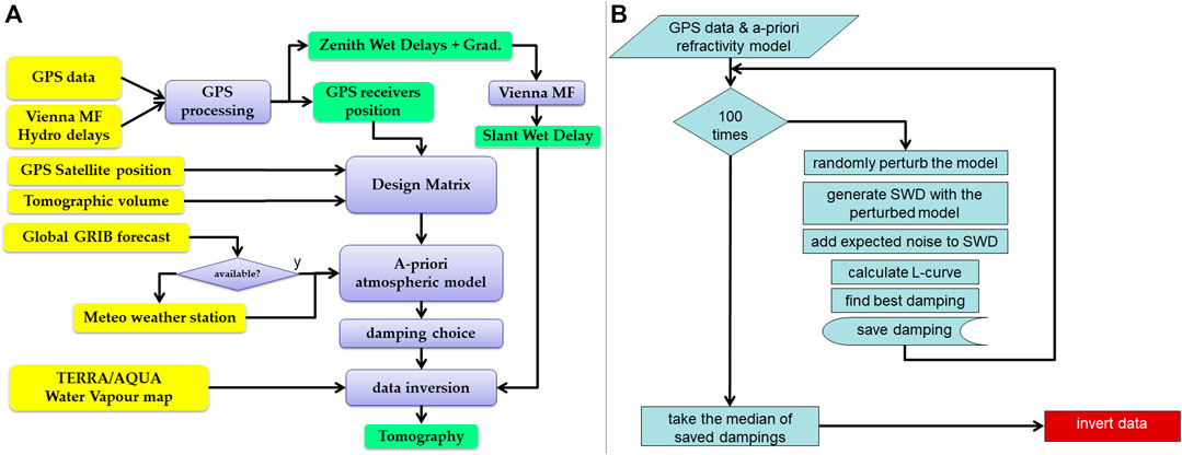
FIGURE 1. (A) Block diagram of the processing chain. In yellow, the blocks with external data; in violet, the processing blocks; in green, the blocks with calculated parameters from GPS and the block of final inversion for tomography calculation. (B) Zoom of the “damping choice” block: flow diagram of the algorithm to estimate a damping factor for a robust tomography. The damping factor followed an iterative process: for each iteration, we selected the best damping factor (by L-curve) to reconstruct a randomly perturbed model where real measured noise was added. The single L-curve was calculated in a fixed set of 10 damping values. At the end of the process, the damping factor used for the real data inversion was the median of the ones obtained from the iterations.

Although the number of rays crossing the voxels exceeds the number of unknowns, the linear system in Eq. 6 is usually underdetermined. This is so because, for example, a voxel in the grid may not be crossed and thus be undetermined. Then, we introduce a regularization process, namely, damped least squares approach (Tarantola, 2005), that minimizes the following cost function:

${\left|SWD-{10}^{-6}A{N}_w\right|}^2+\gamma {\left|{10}^{-6}{N}_w\right|}^2(7)$

Minimizing the first term of the cost function (7) gives the model that better fits the data in the least-squares sense. The regularization term, although introducing biases in solutions, penalizes large solution values; reduces variance, the mean square error; and helps improve the prediction accuracy.

The “damping-factor” γ controls the reduction of variance against an increase of bias (Tarantola, 2005). The damped least square has a closed form solution given by:

${10}^{-6}{N}_w=\left(A^{T}A+\gamma I\right){}^{-1}{A}^{T}SWD(8)$

Where I is the identity matrix.

The most important part in the data inversion algorithm is the choice of the best damping factor that balances solution variance and bias, given the available data.

The “damping-factor” is usually set empirically, by running a series of single iteration inversions aimed at exploring a wide range of damping values, and plotting data misfit vs. model variance L-curve method (Tarantola, 2005; Hirahara, 2000). To make this choice robust to data changes, a Monte Carlo sampling was introduced in the inversion algorithm (see Figure 1B). In particular, for an inversion, 100 synthetic cases are produced at first. Each case consists of a new model generated from the actual a priori model by randomly selecting half of the voxels and modifying the refractivity by superimposing random values whose standard deviation is 10% of their a priori refractivity values (hence, simulating sparse anomalies, difficult to retrieve). For each of the new models, new GPS data are simulated. The simulated data are then added with a Gaussian noise with standard deviation of the same order of magnitude as the associated uncertainties of current measurements. The best damping factor for each synthetic case is retrieved as the coefficient with the minimum residual norm and the minimum norm of refractivity model which corresponds to the point with maximum curvature on the L-curve (Hirahara, 2000; Tarantola, 2005). The final damping factor is chosen as the median of the best factors retrieved from the synthetic cases. This choice allows us to avoid extreme scattered solutions and make solutions robust against changes in data, either GPS network configuration and/or measurement uncertainties, as shown in Aranzulla and Puglisi, 2015.

The N_w refractivity values were finally selected by the method of Toomey and Foulger (1989) and for the Mt. Etna test site (Aranzulla and Puglisi, 2015).

The Atmospheric Model

The atmospheric a priori model we use is divided into layers where atmospheric refractivity varies only with the altitude. In ideal experimental conditions, we can initialize the tomographic model, by computing the refractivity at an arbitrary altitude using the atmospheric measurements of weather balloons, through Eq. 2. In the case of Mt. Etna, the radiosonde data performed in Trapani station are therefore not suitable to describe the actual atmosphere around the volcano, which is located too far away. To overcome this problem, we used two strategies, depending on the data availability for the studied period. For this study, we use the NCEP GFS 0.25° global forecast grid historical archive (NOAA http://dx.doi.org/10.5065/D65D8PWK). In particular, we extract the parameters of Eq. 2 relevant to the 26 physical levels of the NCEP GFS grids, and compute the refractivity at each altitude by averaging the values of adjacent pixels within the investigation volume. However, if NCEP GFS grids are not available, the model is able to predict T, p_d, and p_w at any altitude, and then compute the refractivity profile for the a priori model of atmospheric refractivity, starting from the atmospheric measurements of pressure (p₀), temperature (T₀), and relative humidity (H₀) at the ground level (Saastamoinen 1972a; Saastamoinen, 1972b). Since we cannot exactly know p_w at a defined elevation, we estimated a variation range for that value. Since the highest value of p_w at each height corresponds to the saturated water vapor pressure, we can consider the two extreme cases: the first, called dry condition (which estimates the hydrostatic refractivity N_h) and the second, called saturated condition (which estimates the N_h + N_w(saturated) term of refractivity). Thus, it is possible to calculate the refractivity and consequently the propagation velocity corresponding to different heights from sea level, for the two limit conditions: dry and saturated. Consequently, we are able to evaluate whether or not the refractivity tomography results are physically acceptable solutions.

The Global Positioning System Measurements

Since 2000, a continuous GPS array has operated to monitor the ground deformations of Mt. Etna volcano (Palano et al., 2010). The actual array consists of 42 stations that provide a dense coverage of the volcano (Figure 2).

FIGURE 2

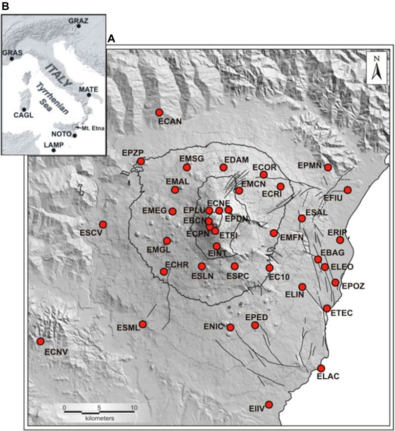
FIGURE 2. (A) The permanent GPS stations over Mt. Etna volcano. 1,000 m contour lines are shown. (B) IGS stations included in the International Terrestrial Reference Frame (ITRF).

Among the whole GPS array, we used a subset of 29 stations where a full data archive is available for the studied period (2015). The stations are equipped with low-multipath choke-ring antennas, and we apply elevation-dependent corrections for the antenna phase centers (Schmid et al., 2005). We processed the GPS data using the GAMIT package developed by the Massachusetts Institute of Technology (Herring et al., 2010). This software uses double-differenced GPS phase observations to estimate for each observing span (in our case 24 h) a single set of station coordinates and orbital parameters together with piecewise linear models of zenith tropospheric delay (ZTD) and gradients at each station. Standard models for precession, nutation, Earth rotation, and solid Earth and ocean tides are applied (IERS Conventions). The motions of the GPS satellites are taken from the Final Orbits of the International GNSS Service (https://www.igs.org/), which typically have an accuracy of ∼2 cm. We processed our data with the data from six surrounding IGS stations (Figure 2), used as reference stations to tie our network to the International Terrestrial Reference Frame (ITRF). Although GAMIT's output separately provides dry and wet tropospheric delay, caused by the high spatial and temporal variability, only the wet component is important for our purposes (Figure 1A). Zenith wet delay (ZWD) is estimated during the GPS processing by assuming a 2-h interval and interpolated through time by a spline approach. Then, the delay along the line of sight between the station and the satellite, slant wet delay (SWD), is computed by properly mapping the zenith wet delay (ZWD) through the so-called Vienna Mapping Function 1 (VMF1) which improves the quality of GPS solutions (Boehm et al., 2006). This estimation process is overall summarized as “Vienna MF” in Figure 1A. We included only data with elevation angle above 15° in order to minimize multipath effects and errors in the mapping functions because, at such elevation, the ray bending effect is negligible. The first-order ionospheric delay is removed by forming the “ionosphere-free” combination of the L1 and L2 phases. After estimating station coordinates and atmospheric parameters from the modeling of the double-differenced phase, GAMIT can produce residuals for the undifferenced phases by estimating clock corrections that the double-difference observations cancel (Alber, et al., 2000). Although the undifferenced post-fit phase residuals and SWD are suitable for atmospheric tomography, we chose to use only the SWD data in order to have a more reliable and stable estimation of the atmospheric effect to EM signal.

Moderate Resolution Imaging Spectroradiometer Data and Integration

The MODIS (Moderate Resolution Imaging Spectroradiometer) instruments operate on board the Aqua and Terra satellites. The sensors collect data in 36 spectral bands within the range 0.4–14.4 µm and at different spatial resolutions (2 bands at 250 m, 5 bands at 500 m and 29 bands at 1 km). The satellites are operated by NASA (https://modis.gsfc.nasa.gov/) and cover the entire Earth every 1–2 days; in particular, the Mt. Etna area is covered two times per day, so these data are particularly suitable for the aim of this study. NASA web services disseminate MODIS data at different levels of processing as well as derived products for land, ocean, and atmospheric applications. The MODIS has the appropriate absorption bands to retrieve water vapor content in the atmospheric column (Spinetti 2004 and Buongiorno, 2007). Here, we use the IPWV (integrated precipitable water vapor) product of the multispectral EO data series that is stored and delivered at 5 km pixel resolution. Figure 3 shows one of MODIS IPWV related to a night passage of the Aqua satellite for the day August 22, 2015.

FIGURE 3

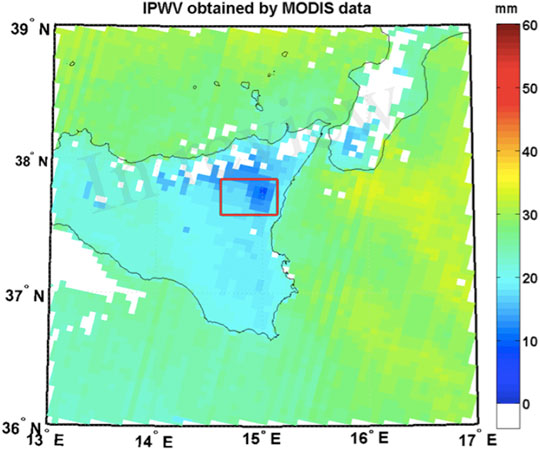
FIGURE 3. IPWV map acquired by the MODIS on August 22, 2015 at 01:10 UTC. The red box indicates the area defined to perform the comparison between MODIS and GPS IPWV. White pixels correspond to no data (clouds).

In order to add these IPWV as observable in our tomographic model of Mt. Etna (Figure 1A), we must first verify that they are consistent with the IPWV values estimated from the processing of our GPS data. The ZWD is directly proportional to Precipitable Water Vapor by a factor calculated during GPS processing (Bevis et al., 1994). The comparison has been performed for the entire year 2015 considering GPS and MODIS-retrieved water vapor data at the same time as satellites pass. In particular, 612 Terra and Aqua satellite acquisitions (both diurnal and nocturnal) were employed in the comparison, and 33 stations of the overall network were considered for GPS measurements.

The comparison was made by averaging the measurements within a considered common area (box in Figure 3). The averages result from all the pixels falling in the box for MODIS data and from all acquisitions by the GPS stations within the same box. Figure 4 shows the comparison results. MODIS data overestimate the GPS ones by ∼7%, and the resulting Pearson correlation is equal to 0.91. Considering these differences, it can be stated that the IPWV measurements derived by MODIS data are usable as input for the tomographic model. Finally, it is worth to note that only the clear sky condition enables obtaining reliable IPWV measurements.

FIGURE 4

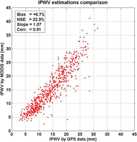
FIGURE 4. Scatterplot of IPWV comparison between MODIS and GPS of one year of data (2015).

We used the daily IPWV data from the MODIS as input for model of Eq. 6 together with SWD from GPS measurements gathered every epoch throughout the day. The SWD was retrieved every 2 h, and we considered the values interpolated by spline. In particular, we considered the mean value of the interpolated SWD in the range ±15 min around the considered time of MODIS acquisition.

Sentinel-1A DInSAR Image

We performed a DInSAR analysis of C-band Sentinel-1-A data referring to selected images acquired between 18 May and November 26, 2015. These data are acquired from the Sentinel-1A satellite operating under the Copernicus program of the European Space Agency (ESA) available from https://scihub.copernicus.eu/dhus/. The processed images were acquired in TopSAR (Terrain Observation with Progressive Scans SAR) Interferometric Wide (IW) mode (VV polarization; vertical transmit and receive polarization), along the descending orbit.

The Sentinel-1A data were processed by GAMMA software (Wegmüller et al., 2015), using a spectral diversity method, and a procedure able to co-register the image pairs with extremely high precision (<0.01 pixel). The interferograms were produced by applying a two-pass DInSAR processing and multi-looking pixels (5 × 1 in range and in azimuth) in order to maintain the full ground resolution (11 × 13 m). The topographic phase was removed from the interferograms by using the SRTM V4 digital elevation model (DEM) generated by Shuttle Radar Topography Mission (SRTM) with three arc-second ground resolution (about 90 m) (Jarvis et al., 2008).

Results and Discussion

The results are divided into two parts. The first subsection concerns the synthetic tests aimed at evaluating if the problem formulation is correct and if the implemented code is suitable to map the refractivity field. In the second subsection, results of selected test cases of 2015 are reported and discussed. Following the results obtained in Aranzulla and Puglisi (2015), the tomographies are computed by using a tomography volume of 54 × 54 × 10 km³, equally spaced in 7 × 7 × 5 voxels centered on the summit craters of Mt. Etna. The tomographic volume setup is shown in Figure 5. We set the lower layer at 1,000 m, rather than 2,000 m as in Aranzulla and Puglisi (2015), in order to maximize the benefit of the use of MODIS data for improving the information about the lowermost layer of the atmosphere (i.e., that with the highest expected water vapor content). We kept the same order of the tomographic matrix used in Aranzulla and Puglisi (2015) (7 × 7 × 5 voxels) because it has proven to be suitable for studying the atmosphere over Mt. Etna with a GPS network composed by 30–40 stations.

FIGURE 5

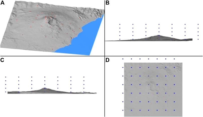
FIGURE 5. 3D Tomographic model 3-D setup; the volume size of 54 × 54 × 10 km is equally spaced in 7 × 7 × 5 voxels centered on Mt. Etna’s summit craters: (A) whole volcano (red dots represent GPS stations); (B) layers on the eastern flank; (C) layers on the northeastern flank; (D) Nadir view. The blue dots represent the voxel centers.

The Synthetic Test

For applying the method described in The Tomography Algorithm, we first need to compute the test's tomography and evaluate the quality of the results. The test has been carried out by using GPS data only, by following the same approach adopted to test a previous tomographic tool implemented by Aranzulla and Puglisi (2015). Because water vapor circulates in the form of bubbles or masses in the atmosphere, we assumed a bubble anomaly structure (i.e., a discretized volume having a shape similar to a bubble), in which the wet refractivity varies by 25% from the surrounding space, with respect to the maximum allowed range (peak to peak value) of the modified layer. Starting from the position of satellites, GPS receivers and the refractivity field containing the “anomaly” (N_perturbed), for the i-th ray, we computed the theoretical slant wet delay (SWD_perturbed) by using Eq. 5 and then, to simulate actual data, adding the noise according to the following equation:

${\text{SWD}}_{\text{noisy}}{=\text{ SWD}}_{\text{perturbed}}+\text{ noise }\left(\text{\%,n}\sigma \right)(9)$

We added a normally distributed random noise of 10% within 2σ, that is, about twice the typical GAMIT SWD error magnitude. The SWD_noisy represents the perturbed and noised slant wet delay value of the ith ray inside the tomography volume. Coming from N_perturbed, SWD_noisy contains the effect of the set perturbation.

Figure 6 shows the tomography results of the bubble structure synthetic test obtained, assuming the GPS array geometry of October 8, 2014 (28 operational stations). By adopting the approach described in Aranzulla and Puglisi (2015), the damping factor value is 18,400, and the spread function (SF) threshold above which the results are valid is 0.8. Figure 6A shows the values of the wet refractivity field (tomography) for all the voxels, while Figure 6B shows the matrices of the assumed perturbation model (bubble) and the tomographic results. Figure 6 allows comparing the tests performed in a synoptic way. The result of the tomography is consistent with the assumed model, that is, the tomography reveals the right perturbations in the right place. The expected (modeled) and estimated (tomographic) values of the refractivity are coincident at the layers 1,000, 5,000, and 7,000 m. Robust conclusions cannot be drawn at the highest and lowest layers. Indeed, at the layer 1,000 m, only one result is acceptable within the fixed thresholds. The statistical reliability of remaining voxels is too low, even though the results are close to the expected model (blue line in Figure 6A). At layer 9,000 m, the estimated anomalies are small as expected (because at that elevation, the temperature is extremely low and the troposphere contains almost no water), but too close to the associated uncertainties, thus preventing any statistical assessment at this elevation.

FIGURE 6

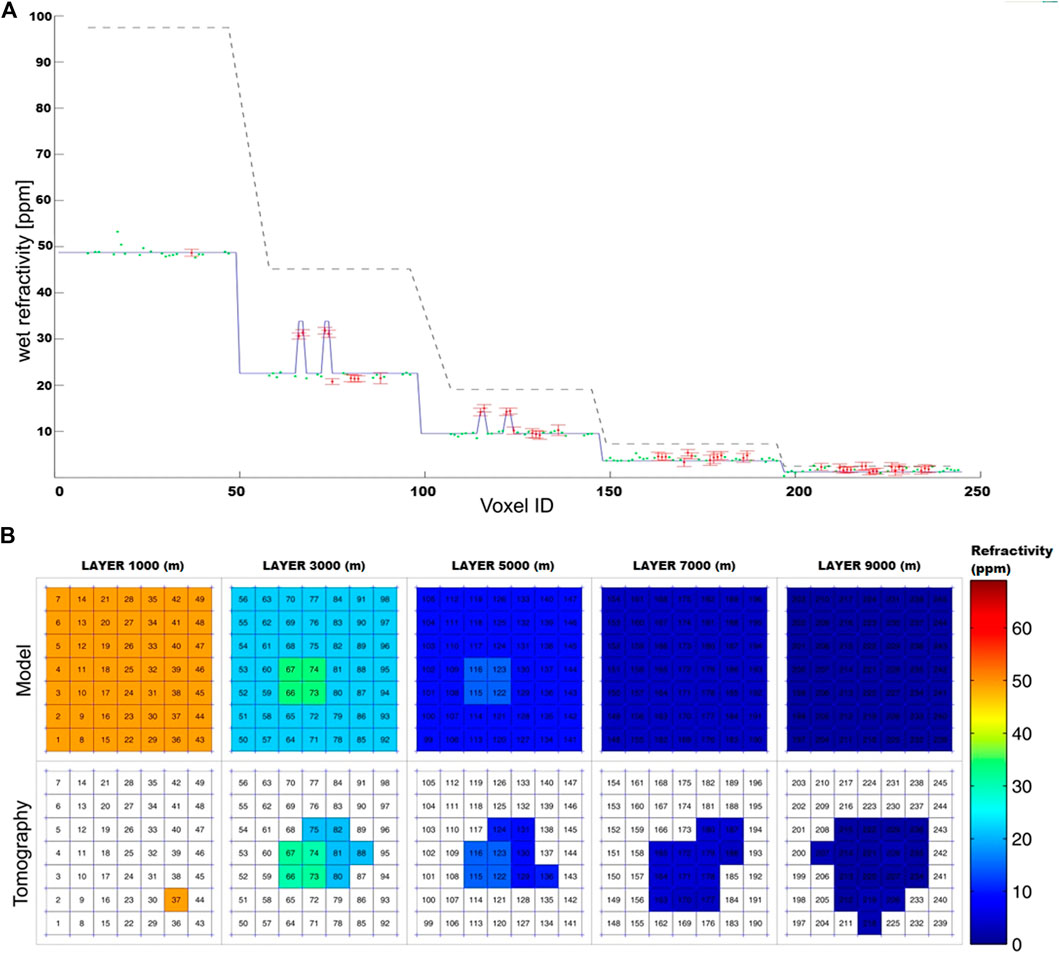
FIGURE 6. (A) Wet refractivity field vs. voxel, ranked according to the position of the voxel in the matrix (B). Dashed black lines represent the physical constraints for the tomographic solution (saturation at the different elevations). The blue line is the wet refractivity starting model. The green points are the numeric results of all the voxels in which it is possible to calculate a refractivity value. The red points represent the refractivity values of the voxels considered to be acceptable according to the fixed thresholds (damping and SF), that is, the result of the tomography. (B) tomography results: the first row refers to the reference model, and the second row is the reconstructed tomography. The voxels are numbered from lower to upper layer and from south to north, in cardinal numbers. The tomography images show only the voxels over the SF threshold, the others are blank. Results are plotted according to the color scale on the right. The considered volume refers to the model shown in Figure 5.

The Actual Tests

The outcomes of the previous section allow us to apply the tomography in real cases of Sentinel-1 interferograms. It is worth noting that for each interferogram, we have to use two tomographies. Five test cases have been selected from the interferograms produced over Mt. Etna by using C-band Sentinel-1A data. Due to the topography of Mt. Etna, the atmospheric artefacts on the interferogram in general have a concentric pattern and high-frequency local perturbation in the north-northeastern flank of the volcano. To select the actual case, we processed all Sentinel-1A available data for 2015 and then identified, by visual inspection criterion, the interferograms with the most evident atmospheric artefacts (Table 1). With reference to the flowchart of Figure 1, starting from the GAMIT GPS ZWD and gradients output, the GPS receiver and satellite positions, the IPWV MODIS data, and the global numerical weather prediction model computed by the U.S. National Weather Service (NWS), we set the tomography volume and computed the A matrix of Eq. 6. Table 1 shows the selected test cases together with GPS at the time of Sentinel-1A passes, the IPWV MODIS data, and the available GPS receiver data. The tomographies were computed considering only the nocturnal acquisitions of the MODIS, as the closest in time to the Sentinel-1A acquisition time. The cloudy sky of 21 October and 26 November compromised the possibility to measure the water vapor content from MODIS data, excluding cloudy areas as observables. This is why the damping factor γ of Eq. 7 is different for those two cases (see Table 1). As previously mentioned, the SF and γ thresholds govern the selection of the representative voxels. The last column of Table 1 represents the percentage of the resolved voxels where the 21 October and 26 November cases show the effect of the lack of MODIS data clearly. Figure 7 shows the tomography results of the actual test cases with the corresponding parameters in Table 1, where it is evident that the number of resolved voxels, and hence the covered area, is greater for 17 July and 22 August. The availability of the retrieved MODIS data also allows computing the voxel refractivities of the western flank of the volcano, especially in the lower layers where the highest contribution of water vapor is expected.

TABLE 1

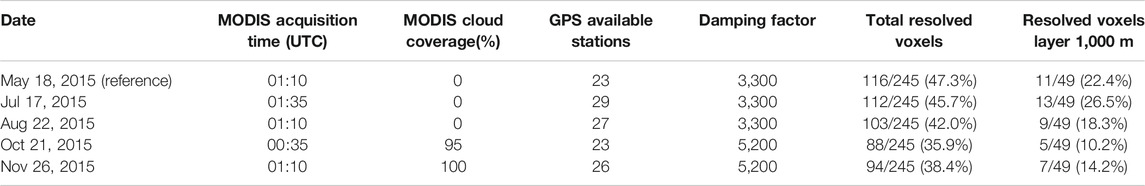
TABLE 1. Selected test cases (UTC hour ranges from 05:04 to 05:06 acquisition time of Sentinel-1A).

FIGURE 7

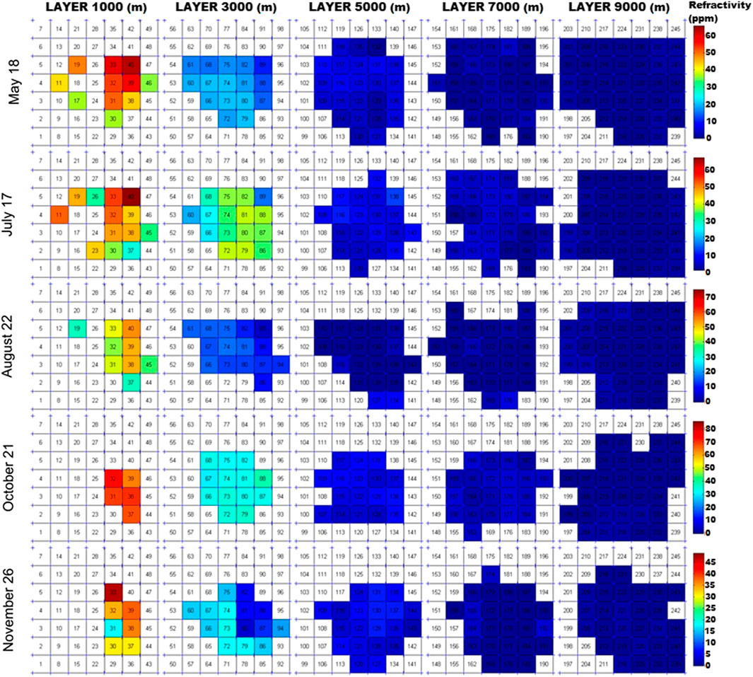
FIGURE 7. Wet refractivity tomography of the selected actual cases. Each test case has a different color scale in order to appreciate the variations of the individual test case.

The number of resolved voxels is statistically greater with the introduction of MODIS data (18 May, 17 July and 22 August) as shown in Table 1, which demonstrates how the addition of the MODIS improves the overall resolution of the tomography. Indeed, the average of the total resolved voxels ranges from 37.1% without MODIS data (cloudy weather conditions) to 45% with MODIS data (clear sky weather conditions), with an increase of 7.9%. In particular, in the lowest layer (1,000 m), the resolved voxel percentage increases on average by 10.2%, from 12.2% without MODIS data to 22.4% with MODIS data. This percentage represents an improvement of about 80% in resolving the voxels of the lowest layer (1,000 m) in relation to the use of GPS data only (Figure 8).

FIGURE 8

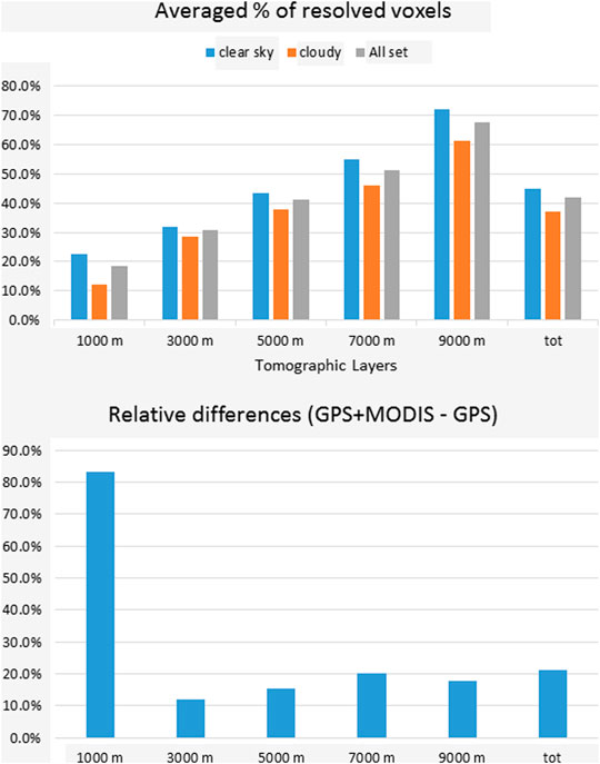
FIGURE 8. Resolved Voxels Statistics. In the upper histogram, the averaged percentage of the resolved voxels are plotted, for the different layers (1,000 m, 3,000 m, 5,000 m, 7,000 m, and 9,000 m) and the whole set of the tomographies; the “clear sky” values refer to the 18 May, 17 July, and 22 August tomographies; the “cloudy” values refer to the 21 October and 26 November tomographies; “all set” values refer to all tomographies. In the lower histogram, the relative difference between “clear sky” (GPS + MODIS) and “cloudy” (GPS) vs. “cloudy” (GPS) tomographies, for the different layers (1,000 m, 3,000 m, 5,000 m, 7,000 m, and 9,000 m) and the whole set of the tomographies.

In order to use the results of tomographies to correct SAR interferograms, it is necessary to calculate the Sentinel-1A line of sight (LOS) delay stored during the whole transition period of the radar signals in the troposphere. To this end, we implemented a specific routine in the tomographic tool, able to compute the LOS delay by Eq. 5 using the obtained refractivity results. As the LOS cannot be calculated without knowing the refractivity value of all the voxels of the investigated volume, it is important to properly set the refractivity values for the unresolved voxels, which were set to the starting values, corresponding to the NCEP grid parameters. Figure 9 shows the wet delay LOS maps referred to Sentinel-1A descending orbit actual cases, computed by using the tomography results.

FIGURE 9

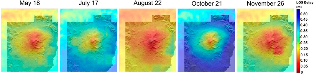
FIGURE 9. Wet delay line of sight maps referred to the five actual cases selected according to Sentinel-1A descending orbit acquisitions.

Finally, we used those wet delay LOS map results of Figure 9 to correct the atmospheric effects in the real SAR interferograms. To do so, such results were converted in four simulated interferograms of differential delay (DInDelay) by adopting a differential approach and by using 18 May as the reference date. Figure 10 shows in the second row the resulting phase of simulated interferograms (DInDelay) together with the corresponding real Sentinel-1A interferograms shown in the first row. In the end, we corrected the phase interferograms by applying the DInDelay to the Sentinel-1A interferograms (third row in Figure 10).

FIGURE 10

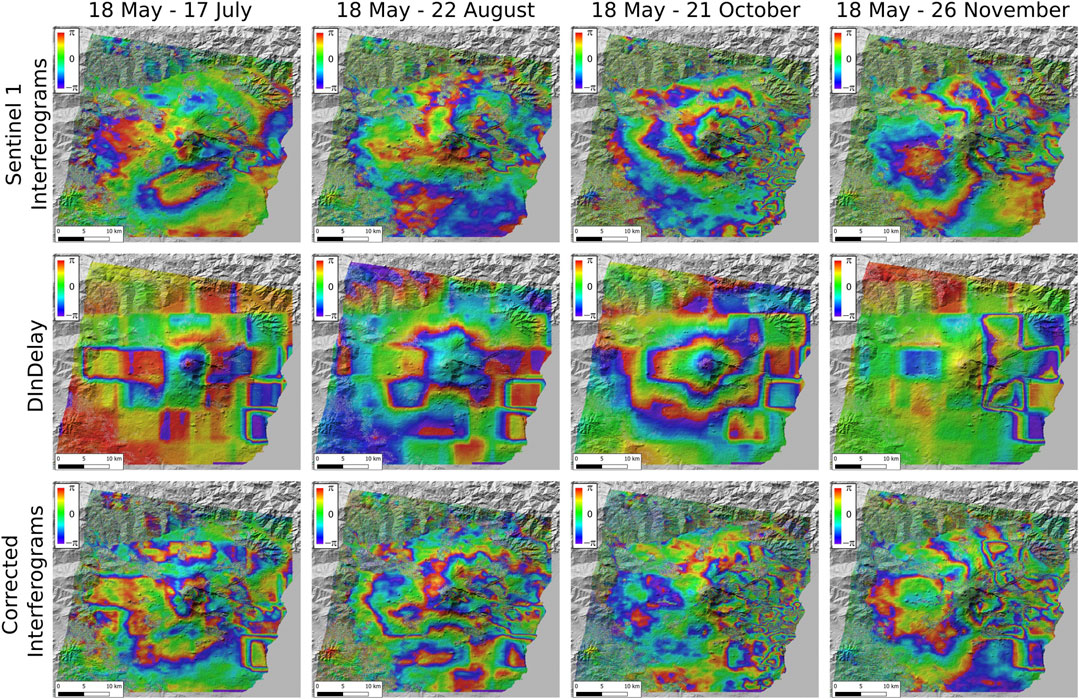
FIGURE 10. Sentinel-1 interferograms, DInDelay (Differential Interferograms Delay) and Sentinel-1 corrected interferograms. On the first row the DInSAR data are shown, on the second and third rows the corresponding DInDelay and corrected interferograms. All the images are shown in phase (−π, π; 2π phase corresponds to 28 mm). In the 18 May–26 November interferogram the high-frequency atmospheric perturbation is in the northeastern flank.

Results shown in Figure 10 allow drawing several observations about the suitability of the proposed tomographic model to correct the DInSAR data and making suggestions for future developments. Besides the differences in the spatial resolution between the Sentinel-1A data and the tomography, due to the intrinsic differences in the pixel sizes in the two datasets, overall, the DInDelay shows the same fringes pattern of the SAR interferograms. It confirms that at the first order, the selected SAR interferograms contain significant atmospheric contributions as we supposed.

The corrected interferograms (third row of Figure 10) show two notable characteristics. 1) The pattern of the fringes often mimics the boundary of the voxels (“boxiness”); this is particularly evident in the south-eastern (along the coast line), western and north-western flanks of the volcano. This effect, which prevents the analysis of subtle “small” features such as local faults, is somewhat expected due to the large dimension of the voxels, and might be overcome in the future by reducing the voxel dimensions. 2) There remains an evident spatial high-frequency perturbation in the right and upper-right part of 18 May–21 October and 18 May–26 November (corresponding to the eastern and northeastern flanks of the volcano). This characteristic indicates that only in these parts of the SAR interferograms are the corrections not appropriate. This was somewhat expected as strong turbulence of the lower atmosphere is often visible in the interferograms of these parts of the volcano. It is worth noting that also MODIS data showed the cloudy weather conditions on those dates (Table 1). This characteristic was not captured by the atmospheric tomography probably because the spatial resolution of our tomography is too poor compared to the small scale of this phenomenon. Just as for the “boxiness,” the high-frequency perturbation can be properly estimated by the reduction of the voxel dimensions to improve the effectiveness of the tomographic correction.

Besides the high-frequency residuals in the eastern and northeastern flanks of the volcano, the application of the atmospheric correction mostly reduces the number of concentric fringes in the corrected interferograms of 18 May–17 July, 18 May–21 October, and 18 May–26 November. The most successful correction is visible in the images relevant to 18 May–21 October. While the original SAR interferogram shows the highest number of fringes (about three fringes) of deformation at the top of the volcano, the DInDelay mimics the pattern of the experimental fringes well, and the corrected interferograms show values varying by about one fringe, especially in the western and southwestern flanks. Only in the southeastern flank do we observe a voxel-shaped anomaly, likely produced by the poor estimation of the atmospheric anomalies in some voxels due to poor GPS network geometry in this area. Indeed, the same voxel-shaped anomaly is observed in the corrected interferograms of 18 May–17 July and 18 May–26 November. The latter shows a residual in the western flank, indicating an approach of the ground surface to the radar sensor which cannot be associated either to the inflation or to the spreading of the volcano, both phenomena often observed in this flank (Bonforte et al., 2008). Indeed, by independently processing the GPS time series for the same period, with GIPSY 6.4 software (https://gipsy-oasis.jpl.nasa.gov/), we cannot observe any significant deformation consistent with these residuals (Figure 11). The maximum deformation in LOS among all the stations is in fact less than 1 cm and is recorded at the ECHR station. Thus, the residuals might be related to turbulent atmosphere that cannot be modeled by the tomography.

FIGURE 11

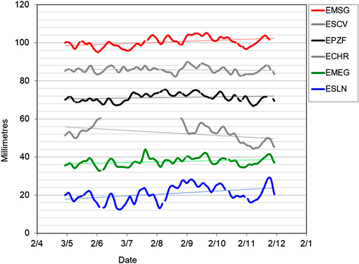
FIGURE 11. GPS LOS displacement time series of the stations located in the western flank of Mt. Etna and their linear trends. For the distribution of the stations refer to Figure 2.

It is worth noting that for all actual cases, except for the 18 May–22 August pair, the slope of the Sentinel-1A experimental fringes is consistent with the slope of the fringes of the model. The inconsistency relevant to the 18 May–22 August pair might be due to non-modeled atmosphere conditions or to pitfalls in the tomographic inversion. Indeed, we noticed that it includes the tomography with the highest refractivity at the 3,000 m layer (Figure 7) due possibly to inaccurate NCEP parameters on 22 August or to fast changes in the lower atmosphere that the time delay between SAR and the MODIS passes cannot take into account.

Conclusion

One of the sources of uncertainty in measuring deformation by using satellite platforms (GPS and SAR) is the effect of the lower atmosphere in the propagation of the EM signals, mainly due to tropospheric water vapor contents. We implemented a new algorithm to perform a 3-D tomography of the wet refractivity by integrating data from GPS, MODIS, and weather models. This algorithm is an improvement on the step forward from a previous tool derived from the seismic tomography (Aranzulla and Puglisi, 2015). The algorithm has been tested and applied to Mt. Etna 2015 test cases. The study shows that by using GPS IPWV alone, the wet refractivity tomography results in about 37% of resolved voxels. Adding MODIS IPWV data increases on average the number of resolved voxels by about 8%. In the lower critical layer (1,000 m), the resolved voxels improve by about 80% in relation to the use of GPS data only. Introducing the GRIB file from NOAA global forecast analysis has allowed us to initialize the tomographic computation with reliable atmospheric conditions and assign the wet refractivity values in the remaining unresolved voxel. One of the main advantages of the availability of a tomographic model of the lower atmosphere is the possibility to estimate the LOS travel time of the SAR signals. To this end, the tomographic tools have been updated with a routine able to compute the LOS delay.

We tested the model by assuming a bubble-shaped anomaly at the lower atmosphere. The simulation shows that the results are consistent with the expected values. Furthermore, the tool has been applied to real Sentinel-1A interferograms during 2015, for which we computed the relevant tomographies, the corresponding wet delays, and the simulated interferograms (DInDelay). The real cases show that often, although in limited areas, the tomography is able to capture the atmospheric effect at the large scale and correct the Sentinel-1A interferograms. This work proves that the proposed method can be used to correct atmospheric effects in areas with prominent topography and on interferograms with severe atmospheric artefacts, even in cloudy conditions. Future studies will allow us to overcome the main limit of the method (e.g., reduction of the voxel dimensions) and to improve its effectiveness, also by including other GNSS constellation data.

Further improvements will be suitable for monitoring active volcanoes worldwide where a local GPS network is operating.

Data Availability Statement

The datasets generated for this study are available on request to the corresponding author.

Author Contributions

MA, CS, FG, GP, and PB contributed conception and design of the study; MA, FC, and VR developed the tool; MA, CS, FC, VR, and FG performed the analysis; MA and CS wrote the first draft of the manuscript; MA, CS, and VR, wrote sections of the manuscript. All authors contributed to manuscript revision, and read and approved the submitted version.

Funding

This study has been carried out in the frame of the EC FP7 Mediterranean Supersite Volcanoes project (ECGA 308665) funded by the European Commission and supported by H2020 EVEREST project funded by the European Commission. Copernicus Sentinel-1 data (2015) are provided by ESA in the framework of GEO-GSNL initiative and available at the Copernicus Open Access Hub (https://scihub.copernicus.eu). The MODIS dataset were acquired by the INGV-ONT real-time KSG multi-mission satellite acquisition system funded by Italian Presidenza del Consiglio dei Ministri – Dipartimento della Protezione Civile (DPC).

Conflict of Interest

The authors declare that the research was conducted in the absence of any commercial or financial relationships that could be construed as a potential conflict of interest.

Acknowledgments

We thank S. Conway for his editing precious help and the Reviewers that help us to substantially improve the work.

References

Alber, C., Ware, R., Rocken, C., and Braun, J. (2000). Obtaining single path phase delays from GPS double differences. Geophys. Res. Lett. 27 (17), 2661–2664. doi:10.1029/2000GL011525

CrossRef Full Text | Google Scholar

Aranzulla, M., and Puglisi, G. (2015). GPS tomography tests for DInSAR applications on Mt. Etna. Ann. Geophys. 58 (3), S0329. doi:10.4401/ag-6750

CrossRef Full Text | Google Scholar

Balal, Y., and Pinhasi, Y. (2019). Atmospheric effects on millimeter and sub-millimeter (THz) satellite communication paths. J. Infrared Millim. Terahertz Waves 40 (2), 219–230. doi:10.1007/s10762-018-0554-7

CrossRef Full Text | Google Scholar

Beauducel, F., Briole, P., and Froger, J. L. (2000). Volcano wide fringes in ERS SAR interferograms of Etna: deformation or tropospheric eect?. J. Geophys. Res. 105, 16391–16402., doi:10.1029/2000JB900095

CrossRef Full Text | Google Scholar

Benevides, P., Catalao, J., Nico, G., and Miranda, P. M. (2018). 4D wet refractivity estimation in the atmosphere using GNSS tomography initialized by radiosonde and AIRS measurements: results from a 1-week intensive campaign. GPS Solut. 22 (4), 91. doi:10.1007/s10291-018-0755-5

CrossRef Full Text | Google Scholar

Benevides, P., Catalao, J., Nico, G., and Miranda, P. M. (2015a). Inclusion of high resolution MODIS maps on a 3D tropospheric water vapor GPS tomography model. in remote sensing of clouds and the atmosphere XX. Inte. Soc. Opt. Photonics 9640, 96400. doi:10.1117/12.2194857

CrossRef Full Text | Google Scholar

Benevides, P., Nico, G., Catalão, J., and Miranda, P. M. (2015b). Bridging InSAR and GPS tomography: a new differential geometrical constraint. IEEE Trans. Geosci. Rem. Sens. 54 (2), 697–702. doi:10.1109/TGRS.2015.2463263

CrossRef Full Text | Google Scholar

Benevides, P., Nico, G., Catalão, J., and Miranda, P. M. (2016). Analysis of Galileo and GPS integration for GNSS tomography. IEEE Trans. Geosci. Rem. Sens. 55 (4), 1936–1943. doi:10.1109/TGRS.2016.2631449

CrossRef Full Text | Google Scholar

Bernot, H., Walpersdorf, A., Reverdy, M., van Baelen, J., Ducrocq, V., Champollion, C., et al. (2014). A GPS network for tropospheric tomography in the framework of the Mediterranean hydrometeorological observatory Cévennes-Vivarais (southeastern France). Atmos. Meas. Tech. 7, 553–578. doi:10.5194/amt-7-553-2014

CrossRef Full Text | Google Scholar

Bevis, M., Businger, S., Herring, T. A., Rocken, C., Anthes, R. A., and Ware, R. H. (1992). GPS meteorology: remote sensing of atmospheric water vapor using the global positioning system. J. Geophys. Res. 97 (D14), 15787–15801. doi:10.1029/92JD01517

CrossRef Full Text | Google Scholar

Bevis, M., Businger, S., Chiswell, S., Herring, T. A., Anthes, R. A., Rocken, C., et al. (1994). GPS meteorology: mapping zenith wet delays onto precipitable water. J. Appl. Meteorol. 33 (3), 379–386. doi:10.1175/1520-0450(1994)033<0379:gmmzwd>2.0.co;2

CrossRef Full Text | Google Scholar

Boehm, J. B., Werl, , and Schuh, H., (2006). Troposphere mapping functions for GPS and very long baseline interferometry from European Centre for Medium-Range Weather Forecasts operational analysis data, J. Geophys. Res. 111, B02406. doi:10.1029/2005JB003629

CrossRef Full Text | Google Scholar

Bonforte, A., Ferretti, A., Prati, C., Puglisi, G., and Rocca, F. (2001). Calibration of atmospheric eects on SAR interferograms by gps and local atmosphere models: rst results. J. Atmos. Sol. Terr. Phys. 63, 1343–1357. doi:10.1016/s1364-6826(00)00252-2

CrossRef Full Text | Google Scholar

Bonforte, A., Bonaccorso, A., Guglielmino, F., Palano, M., and Puglisi, G. (2008). Feeding system and magma storage beneath Mt Etna as revealed by recent inflation/deflation cycles. J. Geophys. Res. 113, B05406. doi:10.1029/2007JB005334

CrossRef Full Text | Google Scholar

Bruno, V., Aloisi, M., Bonforte, A., Immè, J., and Puglisi, G. (2007). Atmospheric anomalies over mt. Etna using GPS signal delays and tomography of radio wave velocities. Ann. Geophys. 50 (2), 267–282. doi:10.4401/ag-4417

Google Scholar

Champollion, C., Flamant, C., Bock, O., Masson, F., Turner, D., and Weckwerth, T. (2009). Mesoscale GPS tomography applied to the 12 June 2002 convective initiation event of IHOP_2002. Q. J. R. Meteorol. Soc. 135 (640), 645–662. doi:10.1002/qj.386

CrossRef Full Text | Google Scholar

Chen, B., and Liu, Z. (2014). Voxel-optimized regional water vapor tomography and comparison with radiosonde and numerical weather model. J. Geodes. 88 (7), 691–703. doi:10.1007/s00190-014-0715-y

CrossRef Full Text | Google Scholar

Curlander, J. C., and McDonough, (1991). Synthetic aperture radar: Wiley Interscience. New York, Vol. 11.

Google Scholar

Debye, P. (1929). Polar molecules. New York: Dover.

Google Scholar

Delacourt, C., Briole, P., and Achache, J. (1998). Tropospheric corrections of SAR interferograms with strong topography, application to Etna. Geophys. Res. Lett. 25, 2849–2852. doi:10.1029/98gl02112

CrossRef Full Text | Google Scholar

Essen, L., and Froome, K. D. (1951). The refractive indices and dielectric constants of air and its principal constituents at 24,000 mc/s. Proc. Phys. Soc. B 64 (10), 862–875. doi:10.1088/0370-1301/64/10/303

CrossRef Full Text | Google Scholar

Flores, A., De Arellano, J.-G., Gradinarsky, L. P., and Rius, A. (2001). Tomography of the lower troposphere using a small dense network of GPS receivers. IEEE Trans. Geosci. Rem. Sens. 39 (2), 439–447. doi:10.1109/36.905252

CrossRef Full Text | Google Scholar

Flores, A., Ruffini, G., and Rius, A. (2000). 4D tropospheric tomography using GPS slant wet delays. Ann. Geophys. 18 (2), 223–234. doi:10.1007/s00585-000-0223-7

CrossRef Full Text | Google Scholar

Gradinarsky, L. P., and Jarlemark, P. (2004). Groundbased GPS tomography of water vapor: analysis of simulated and real data. J. Meteorol. Soc. Jpn. 82 (1B), 551–560. doi:10.2151/jmsj.2004.551

CrossRef Full Text | Google Scholar

Healy, S. B. (2011). Refractivity coecients used in the assimilation of GPS radio occultation measurements. J. Geophys. Res. 116, 1–10. doi:10.1029/2010JD014013

CrossRef Full Text | Google Scholar

Herring, T. A., King, R. W., and McClusky, S. C. (2010). Gamit reference manual, release 10.4. Cambridge, MA, USA: Massachusetts Institute of Technology.

Google Scholar

Heublein, M., Alshawaf, F., Erdnüß, B., Zhu, X. X., and Hinz, S. (2019). Compressive sensing reconstruction of 3D wet refractivity based on GNSS and InSAR observations. J. Geodes. 93 (2), 197–217. doi:10.1007/s00190-018-1152-0

CrossRef Full Text | Google Scholar

Hill, R. J., Lawrence, R. S., and Priestley, J. T. (1982). Theoretical and calculation aspects of the radio refractive index of water vapor. Radio Sci. 17 (5), 1251–1257. doi:10.1029/RS017i005p01251

CrossRef Full Text | Google Scholar

Hirahara, K. (2000). Local gps tropospheric tomography, Earth. Planets Space 52 (11), 935–939. doi:10.1186/BF03352308

CrossRef Full Text | Google Scholar

Hofmann-Wellenhof, B., Lichtenegger, H., and Collins, J. (2001). Global positioning system: theory and practice. 5th Edn. Verlag Wien, New York: Springer.

Google Scholar

Hopfield, H. S. (1969). Oceans and atmospheres, 4487-4499. Two-quartic tropospheric refractivity profile for correcting satellite data. J. Geophys. Res. 74, 18. doi:10.1029/JC074i018p04487

CrossRef Full Text | Google Scholar

Ichikawa, R., Kasahara, M., Mannoji, N., and Naito, I. (1995). Estimations of atmospheric excess path delay based on three-dimensional numerical prediction model data. J. Geod. Soc. 41 (4), 379–408. doi:10.11366/sokuchi1954.41.379

CrossRef Full Text | Google Scholar

Jarvis, A., Reuter, H. I., Nelson, A., and Guevara, E. (2008). Hole-filled SRTM for the globe version 4, available from the CGIAR-CSI SRTM 90m Database. Available at: http://srtm.csi.cgiar.org. (Accessed January 15, 2016).

Google Scholar

Kämpfer, N. (2012). Monitoring atmospheric water vapor, New York, NY: Springer Vol. 2012, 326.

Google Scholar

Karmakar, P. K. (2017). Microwave propagation and remote sensing: atmospheric influences with models and applications. Boca Raton, Florida, United States: CRC Press.

Google Scholar

Massonnet, D., Rossi, M., Carmona, C., Adragna, F., Peltzer, G., Feigl, K., et al. (1993). The displacement eld of the landers earthquake mapped by radar interferometry. Nature 364, 138–142. doi:10.1038/364138a0

CrossRef Full Text | Google Scholar

Nilsson, T., and Elgered, G. (2007). Water vapor tomography using GPS phase observations: results from the ESCOMPTE experiment. Tellus Dyn. Meteorol. Oceanogr. 59 (5), 674–682. doi:10.1111/j.1600-0870.2007.00247.x

CrossRef Full Text | Google Scholar

Nilsson, T., Böhm, J., Wijaya, D. D., Tresch, A., Nafisi, V., and Schuh, H. (2013). “Path delays in the neutral atmosphere”. in Atmospheric effects in space geodesy, Berlin, Heidelberg: Springer 73–136.

CrossRef Full Text | Google Scholar

Notarpietro, R., Cucca, M., Gabella, M., Venuti, G., and Perona, G. (2011). Tomographic reconstruction of wet and total refractivity fields from GNSS receiver networks. Adv. Space Res. 47 (5), 898–912. doi:10.1016/j.asr.2010.12.025

CrossRef Full Text | Google Scholar

Palano, M., Rossi, M., Cannavò, F., Bruno, V., Aloisi, M., Pellegrino, D., et al. (2010). A geodetic reference frame for mt. Etna GPS networks. Ann. Geophys. Italy 53, 49–57. doi:10.4401/ag-4879

CrossRef Full Text | Google Scholar

Perler, D., Geiger, A., and Hurter, F. (2011). 4D GPS water vapor tomography: new parameterized approaches. J. Geodes. 85 (8), 539–550. doi:10.1007/s00190-011-0454-2

CrossRef Full Text | Google Scholar

Rocken, C., van Hove, T., Johnson, J., Solheim, F., Ware, R., Bevis, M., et al. (1995). GPS/STORM—GPS sensing of atmospheric water vapor for meteorology. J. Atmos. Ocean. Technol. 12 (3), 468–478. doi:10.1175/1520-0426(1995)012<0468:gsoawv>2.0.co;2

CrossRef Full Text | Google Scholar

Rueger, J. M. (2002a). “Refractive index formulae for radio waves,” in Proc. XXII FIG international congress American Society for Photogrammetry and Remote Sensing (Kansas, USA: Addison-Wesley Publishing Company Advanced Book Program/World Science Division). Available at: https://www.fig.net/resources/proceedings/fig_proceedings/fig_2002/Js28/JS28_rueger.pdf.

Google Scholar

Rueger, J. M. (2002b). Refractive indices of light, infrared and radio waves in the atmosphere, Technical report the university of new south wales, Australia. School of Surveying and Spatial Information Systems, Technical Paper Unisurv S-68.

Google Scholar

Saastamoinen, J. (1972a). Introduction to practical computation of astronomical refraction. Bull. God. 106, 383–397. doi:10.1007/BF02522047

CrossRef Full Text | Google Scholar

Saastamoinen, J. (1972b). “Atmospheric correction for the troposphere and stratosphere in radio ranging of satellites,” in The use of artificial satellites for geodesy. Editors S. W. Henriksen, A. Mancini, and B. H. Chovitz (Wiley: New York), 247–251.

Google Scholar

Schmid, R., Rothacher, M., Thaller, D., and Steigenberger, P. (2005). Absolute phase center corrections of satellite and receiver antennas. Impact on GPS solutions and estimation of azimuthal phase center variations of the satellite antenna. GPS Solut. 9, 283–293. doi:10.1007/s10291-005-0134-x

CrossRef Full Text | Google Scholar

Solheim, F. S., Vivekanandan, J., Ware, R. H., and Rocken, C. (1999). Propagation delays induced in GPS signals by dry air, water vapor, hydrometeors, and other particulates. J. Geophys. Res. 104 (D8), 9663–9670. doi:10.1029/1999jd900095

CrossRef Full Text | Google Scholar

Spinetti, C., and Buongiorno, M. F. (2007). Volcanic Aerosol Optical Characteristics of Mt. Etna Tropospheric Plume Retrieved by Means of Airborne Multispectral Images, J Atmos. and Solar-Terrestrial Physic. 69 (9) 981–994.doi:10.1016/j.jastp.2007.03.014

Google Scholar

Spinetti, C., and Buongiorno, M. F. (2004). “Volcanic water vapor abundance retrieved by using hypespectral Data,” in IEEE International Geoscience and Remote Sensing Symposium, Sept 2004, Anchorage, Alaska, USA, 1487–1490. doi:10.1109/IGARSS.2004.1368702

Google Scholar

Tarantola, A. (2005). Inverse problem theory and methods for model parameter estimation, Philadelphia, USA: Society of Industrial and Applied Mathematics (SIAM), 342. doi:10.1137/1.978089871792

Google Scholar

Thayer, G. D. (1974). An improved equation for the radio refractive index of air. Radio Sci. 9 (10), 803–807. doi:10.1029/RS009i010p00803

CrossRef Full Text | Google Scholar

Toomey, D., and Foulger, G. (1989). Tomographic inversion of local earthquake data from the hengill-grensdalur central volcano complex, Iceland. J. Geophys. Res. 94, 497–510. doi:10.1029/jb094ib12p17497

CrossRef Full Text | Google Scholar

Tregoning, P., Boers, R., O'Brien, D., and Hendy, M. (1998). Accuracy of absolute precipitable water vapor estimates from GPS observations. J. Geophys. Res. Atmosphere 103 (D22), 28701–28710. doi:10.1029/98jd02516

CrossRef Full Text | Google Scholar

Ulaby, F. T., Moore, R. K., and Fung, A. K. (1981). “Volume 1-Microwave remote sensing fundamentals and radiometry active and passive,” in Book microwave remote sensing.

Google Scholar

Wadge, G., Webley, P., James, I. N., Bingley, R., Dodson, A., Waugh, S., et al. (2002). Atmospheric models, GPS and InSAR measurements of the tropospheric water vapor field over mount Etna. Geophys. Res. Lett. 29 (19), 11-1–11-4. doi:10.1029/2002gl015159

CrossRef Full Text | Google Scholar

Webley, P., Wadge, G., and James, I. N. (2004). Determing radio wave delay by non-hydrostatic atmospheric modelling of water vapor over mountains. Phys. Chem. Earth 29, 139–148. doi:10.1016/j.pce.2004.01.013

CrossRef Full Text | Google Scholar

Wegmüller, U., Werner, C., Strozzi, T., Wiesmann, A., Frey, O., and Santoro, M. (2015). “Sentinel-1 support in the GAMMA software,” in Proceedings of fringe 2015: advances in the science and applications of SAR interferometry and sentinel-1 InSAR workshop, ESA ESRIN, Frascati, Italy, March 2015 23–27.

Google Scholar

Williams, S., Bock, Y., and Fang, P. (1998). Integrated satellite interferometry: tropospheric noise and gps estimates and implications for interferometric synthetic aperture radar products. J. Geophys. Res. 103 (B1127), 27051–27067. doi:10.1029/98jb02794

CrossRef Full Text | Google Scholar

Zebker, H. A., Rosen, P. A., and Henseley, S. (1997). Atmospheric eects in interferometric synthetic aperture radar surface deformation and topographic maps. J. Geophys. Res. 102 (B4), 7547–7563. doi:10.1029/96JB03804

CrossRef Full Text | Google Scholar

Zhao, Q., Yao, Y., Cao, X., and Yao, W. (2019). Accuracy and reliability of tropospheric wet refractivity tomography with GPS, BDS, and GLONASS observations. Adv. Space Res. 63 (9), 2836–2847. doi:10.1016/j.asr.2018.01.021

CrossRef Full Text | Google Scholar