Integration of Soft Data Into Geostatistical Simulation of Categorical Variables

1 Introduction

In many hydrogeological modeling applications, much of the available characterization data for categorical variables, such as lithology, texture, or hydrofacies, are uncertain or less than 100% accurate. In some geostatistical applications, the categorical data such as soil texture are treated as 100% accurate or “hard” data despite the fact these data are uncertain for various reasons (Carle, 1996; Burow et al., 1997; Carle et al., 1998; Weissmann et al., 1999). In other applications, uncertain or indirect “soft” data such as geophysical imaging are available but found difficult to apply as “soft conditioning” to geostatistical simulations of categorical variables (Falivene et al., 2007; Koch et al., 2014). Categorization of hydrogeological variables often has uncertainty attributable to sample quality, geologic interpretation, or indirectness of measurement (e.g., geophysical logs, cone penetrometer data). For example, so-called “driller’s logs” or lithologic descriptions by well drillers based on interpretations of drilling conditions, cuttings, and limited core samples are, understandably, uncertain (Oatfield and Czarnecki, 1989; Smith, 2002; Dumedah and Schuurman, 2008; Arihood, 2009; Tsai and Elshall, 2013). Yet driller’s logs may provide the most detailed characterization information available for many local site to basin-scale hydrogeological modeling applications (Ezzedine et al., 1999; Weissmann et al., 1999; Weissmann and Fogg, 1999; Carle et al., 2006; Fleckenstein et al., 2006; Elshall et al., 2013). Alternatively, hydrogeological categories can be inferred from geophysical measurements or imaging, but the resulting inferences are inherently uncertain. Paradis et al. (2015) found that even after application of sophisticated machine learning techniques to cone penetrometer test and soil moisture and resistivity probe data, classification errors persist in hydrofacies identification. The resolution of geophysical images varies as a result of petrophysical relationships and, therefore, provides indirect contraints on lithology, texture, or hydrofacies, as further discussed in application of three-dimensional resistivity maps derived from airborne electromagnetic surveys to characterization of spatial occurrences of sand-clay textures (Koch et al., 2014; Hoyer et al., 2015) and electrical resistance tomographs to determine spatial distributions of alluvial or fluvial hydrofacies (Carle et al., 1999; Carle and Ramirez, 1999; Hermans and Irving, 2017). It is a well-accepted fact in the Earth sciences that uncertainty is common to subsurface data.

A general framework for integrating soft data into categorical geostatistical simulation should be useful to stochastic subsurface characterization and inversion of discrete heterogeneity within hydrogeologic systems. One, two, or three-dimensional (3-D) spatial information derived from geophysical imaging or logging (e.g., seismic, electrical) or hydrogeologic interpretation (e.g., cross-sections or calibrated flow models) could be treated as a type of soft data available for conditioning geostatistical simulation of categorical variables. In stochastic inversion, a general framework for integrating prior information could be used, for example, to selectively manipulate discrete heterogeneity structure, such as the interconnectivity of permeable units or the continuity of impermeable units (Carle and Ramirez, 1999; Carle et al., 1999; Aines et al., 2002; Wainwright et al., 2014). A “Markov-Bayes” approach has been proposed to transform the soft data to prior probability distributions (Zhu, 1991; Deutsch and Journel, 1998), but this approach has been deemed intractable because of nonlinear relationships and large volumetric scale of the soft data (Deutsch and Wen, 2000).

Categorical or “indicator” bivariate geostatistical approaches have long been recognized as offering realistic and practical means for assessing the impact of subsurface heterogeneity on field- and basin-scale flow and transport processes (Poeter and Townsend, 1994; McKenna and Poeter, 1995; Poeter and McKenna, 1995; Tsang et al., 1996). As part of the T-ProGS software package (Carle, 1999; Carle, 2007), the tsim code was developed to take advantage of the interpretability of transition probability statistic to ensure that spatial cross-correlations and juxtapositional tendencies of hydrogeologic units or hydrofacies are fully considered in categorical stochastic simulation (Carle, 1996; Carle, 1997; Carle and Fogg, 1996; Carle and Fogg, 1997). The tsim code was modified from the variogram-based sisim code (Deutsch and Journel, 1992; Deutsch and Journel, 1998) in three main ways: 1) formulation of the estimate of the local probability of occurence of a discrete category by a cokriging system of equations instead of multiple indicator kriging equations (Carle and Fogg, 1996), 2) addition of a simulated quenching step to improve match of simulated and modeled simulated variability (Carle, 1997), and 3) addition of an option to vary the local direction of anisotropy direction (Carle, 1996; Carle, 1999; Carle, 2007). The latter modification enables simulation of curvilinear features such as variable stratigraphic dip, major direction of anistropy, and sinuous meandering of fluvial facies (Carle et al., 1998; Tompson et al., 1999; Carle et al., 2006; Green et al., 2010; Engdahl et al., 2012). These modifications were made to improve the ability of geostatistical methods to simulate realistic three-dimensional alluvial or fluvial hydrofacies architecture that influences site-scale flow and transport behavior (Fogg, 1986; Tompson et al., 1999; Fogg et al., 2000; Labolle and Fogg, 2001). Another development of the T-ProGS simulation environment is that it leverages the geologic reality that the spatial variability of many hydro- or geo-facies systems can be characterized by a continuous-lag Markov chain, which provides an intuitive yet statistically rigorous framework for developing geologically realistic models with a minimal number of parameters (Vistelius, 1949; Krumbein and Dacey, 1969; Harbaugh and Bonham-Carter, 1970; Agterberg, 1974; Doveton, 1994; Carle and Fogg, 1997). However, the user of tsim can choose to implement other 3-D models of the transition probability, if so desired (Carle, 1999; Carle, 2007).

The tsim code and its associated transition probability-based categorical geostatistical methodologies have subsequently been found to be useful to characterization and modeling of a variety of heterogeneous hydrogeological systems (Carle, 2000; Ritzi, 2000; Lu and Zhang, 2002; Lu et al., 2002; Bohling and Dubois, 2003; Zhang and Fogg, 2003; Carle et al., 2004; James, 2004; Troldborg, 2004; Weissmann et al., 2004; McDonald et al., 2005; Ye and Khaleel, 2008; Janza, 2009; Sakaki et al., 2009; Alberto, 2010; Engdahl et al., 2010b; Janza, 2009; Doherty and Christensen, 2011; Papapetrou and Theodossiou, 2012; Purkis et al., 2012; Guastaldi et al., 2014; He et al., 2015; Song et al., 2015; Weissmann et al., 2015; Krage et al., 2016; Zhu et al., 2016a; Meirovitz et al., 2017; Muskus and Falta, 2018; Erdal et al., 2019; Sun et al., 2019; Wu et al., 2019; Arshadi et al., 2020). Furthermore, tsim has been applied to the study of a range of problems and processes involving subsurface heterogeneity including groundwater recharge or river flow loss (Tompson et al., 1999; Izbicki, 2002; Fleckenstein et al., 2006; Frei et al., 2009; Engdahl et al., 2010a, Pryshlak et al., 2015; Ganot et al., 2018; Maples et al., 2019, Maples et al.,2020), integration of geophysical data or imaging (Carle and Ramirez, 1999; Carle et al., 1999; Zhu et al., 2016b), aquifer or pore system interconnectivity, percolation, and preferential flow (Fogg et al., 2000; Proce et al., 2004; Harter, 2005; Knudby et al., 2006; Bianchi et al., 2011; Huang et al., 2012), risk analysis (Maxwell et al., 2000; Maxwell et al., 2008), heterogeneity effects on groundwater flow (Lu et al., 2001; Jones et al., 2002; Phillips et al., 2007; Traum et al., 2014; Bianchi, 2017; Liao et al., 2020), heterogeneity effects on contaminant transport (Pawloski et al., 2001; Tompson et al., 2002; Hu et al., 2003; Maxwell et al., 2003; Zhang and Fogg, 2003; Pozdniakov et al., 2005; Zhang et al., 2007; Sivakumar et al., 2005a; Sivakumar et al., 2005b; Carle et al., 2006; Maji and Sudicky, 2008; Sun et al., 2008; Ye et al., 2009; Cooper et al., 2010; Baidariko and Pozdniakov, 2011; Zhang and Meerschaert, 2011; Pozdniakov et al., 2012; Zhang et al., 2013; Glinskii et al., 2014; Liu et al., 2014; Zhang et al., 2014; Beisman et al., 2015; Bianchi et al., 2015; Lu et al., 2015; Maghrebi et al., 2015; Siirila-Woodburn and Maxwell, 2015; Siirila-Woodburn et al., 2015; Mi et al., 2016; Bianchi and Pedretti, 2017; Giraldo et al., 2017; Soltanian et al., 2017a; Teramoto et al., 2017; Chen et al., 2018; Guo et al., 2019b; Guo et al., 2019c; Vincent Henri and Harter, 2019; Guo et al., 2020), efficacy of remediation (Labolle and Fogg, 2001; Lee, 2004; Misut, 2014; Abriola et al., 2019; Guo et al., 2019a), effects of diffusion, dispersion, or fractionation on groundwater tracers (Labolle and Fogg, 2001; Weissmann et al., 2002; Labolle et al., 2006; Labolle et al., 2008; Green et al., 2010; Green et al., 2014; Engdahl et al., 2012; Yin et al., 2020), sequestration of carbon dioxide (Hovorka et al., 2001; Doughty and Pruess, 2004; Ramirez et al., 2006; Ramirez et al., 2010; Deng et al., 2012; Espinet et al., 2013; Sun et al., 2013; Yang et al., 2013; Carroll et al., 2014; Mansoor et al., 2014; Mukhopadhyay et al., 2015; Bianchi et al., 2016; Kitanidis, 2016; Soltanian et al., 2016; Trainor-Guitton et al., 2016; Amooie et al., 2017; Soltanian et al., 2017b; Damico et al., 2018; Buscheck et al., 2019; Yang et al., 2019; Yang et al., 2020), stochastic inversion of hydrofacies spatial distributions, hydraulic properties, or transport behavior (Aines et al., 2002; Jones et al., 2003; Harp et al., 2008; Bohling and Butler, 2010; Harp and Vesselinov, 2010; Blessent et al., 2011; Espinet and Shoemaker, 2013; Berg and Illman, 2015; Wang et al., 2017; Lee et al., 2018; Song et al., 2019), spatial variability of reactive mineral assemblages (Carle et al., 2002; Deng et al., 2010), analysis of contaminant plumes (Reed et al., 2004; Maji et al., 2006; Maji and Sudicky, 2008), assessment of nitrate contamination, reduction, and removal (Carle et al., 2004; Carle et al., 2006; Hansen et al., 2014; Sawyer, 2015; Wallace et al., 2020), permeability structure within fractured rock (Park et al., 2004; Blessent et al., 2011; Blessent, 2013), 3-D modeling of ore-grade distributions (Fisher et al., 2005), probabilistic well location (Stevick et al., 2005), non-point source contamination (Zhang et al., 2006; Refsgaard et al., 2014; Zhang et al., 2018), upscaling of flow and transport parameters (Dai et al., 2007; Fleckenstein and Fogg, 2008; Bakshevskaia and Pozdniakov, 2016), geotechnical engineering (Beretta and Felletti, 2007; Felletti and Berretta, 2009; Zetterlund et al., 2011; Grasmick et al., 2020), assessment of nuclear waste disposal (Back and Sundberg, 2007), effects of subsurface heterogeneity on remote sensing (Eslinger et al., 2007), wellhead protection and contamination vulnerability (Burow et al., 2008; Heywood, 2013; Yager and Heywood, 2014; Theodossiou and Fotopoulou, 2015), physical and chemical heterogeneity in streambeds and the hyporheic zone (Schornberg et al., 2010; Faulkner et al., 2012; Zhou et al., 2014; Pryshlak et al., 2015; Singh et al., 2018; Pescimoro et al., 2019; Liu et al., 2020), effects of micro-topography on surface-subsurface exchange (Frei et al., 2010), analysis of transport at the macrodispersion experiment site (Bianchi et al., 2011; Zheng et al., 2011; Bianchi and Zheng, 2016; Pedretti and Bianchi, 2018; Yin et al., 2020), 3-D soil texture (Haugen et al., 2011; Roig-Silva et al., 2012; Li et al., 2014b), characterization of groundwater ecosystems (Larned, 2012), effects of petroleum reservoir heterogeneity (Purkis et al., 2012; Kwon et al., 2017), geologic units of the Swiss Jura (Sartore, 2013), groundwater hydrology of fens (Sampath et al., 2015; Sampath et al., 2016), potential for liquefaction (Munter et al., 2016; Munter et al., 2017; Boulanger et al., 2019), coupled surface and subsurface flow (Blessent et al., 2017; Erdal et al., 2019), and geomechanical modeling of land subsidence (Zhu et al., 2020). Given the usefulness of the tsim algorithm, which was originally designed for categorical stochastic simulation with conditioning by hard data only, an improved capability to assimilate conditioning from soft data or prior information of variable quality is expected to be useful to hydrogeological and related subsurface applications and research.

In this paper, a simple theoretical framework is developed for incorporating uncertain, indirect, or soft categorical data into categorical geostatistical simulation. Geostatistical realizations will honor or be conditional to both hard and soft data. The theory considers that soft data should not be treated the same as hard data in formulating (co)kriging equations and objective functions in simulated annealing (or quenching) as implemented in the original categorical stochastic simulation codes using bivariate spatial statistics such as isim3d (Gomez-Hernandez and Srivastava, 1990), tsim (Carle 1996; Carle et al., 1998), sisim and anneal (Deutsch and Journel, 1998), and iksim (Ying, 2000).

A new version of tsim, called tsim-s, has been coded to enable incorporation of soft categorical data or prior information. The tsim-s algorithm was originally conceived to enable tsim to produce and perturb stochastic realizations for Monte Carlo Markov chain inversion (Aines et al., 2002; Carle, 2003; Glaser et al., 2004). The new capabilities in tsim-s have more general applicability and flexibility to handle conditioning data of variable quality or uncertainty. tsim-s will be made available by request as the open-source fortran code tsim has been distributed in the past. The development of the equations necessary for implementation of the tsim-s algorithm are included in this paper to fully document the methods and to facilitate coding of the tsim algorithms in higher-level languages such as R (Sartore, 2013; Sartore et al., 2016). As will be seen in the equations, the computational overhead for tsim-s is not signifcantly different from tsim because the only modifications are to the entries in the cokriging matrices and the parameters of the quenching objective function.

This paper provides the theory behind the tsim-s algorithms and results from example applications. The paper first reviews transition probability-based indicator geostatistical theory implemented in the tsim algorithms. Next, the paper derives the equations used for implementing the new soft data capabilities to account for uncertainty in categorical variables using the “hardness” concept previously introduced for continuous variables (Deutsch and Wen, 2000). Cokriging equations and simulated quenching objective functions are re-ormulated to account for soft data using the hardness concept. Example applications are given for hard and soft conditioning at boreholes and from prior conditioning by an array of data such as another realization or a depth-dependent uncertainty function. Results of a 3-D simulation by Carle et al. (2006) are included to demonstrate that tsim-s can be used to produce large-scale stochastic realizations useful for investigation of flow and transport processes in hydrogeologic systems. These examples are provided to show the flexibility of the algorithm and by no means cover all potential applications, a topic that is beyond the scope of this paper. Further discussion is added to clarify the capabilities and limitations of the tsim and tsim-s algorithms in relationship to variogram-based and multi-point geostatistical methods and the current understanding of how the simulation algorithms can and should be implemented in a geological context.

2 Materials and Methods

2.1 Transition Probability-Based Indicator Geostatistics

Transition probability-based indicator geostatistics is a categorical geostatistical approach where the transition probability bivariate statistic is used to analyze spatial variability and formulate cokriging equations (Carle and Fogg, 1996). The transition probability approach enables consideration of spatial cross correlations (e.g., how different facies tend to locate in space relative to each other) and facilitates a Markov chain modeling framework that can be linked to geologic interpretation (Krumbein and Dacey, 1969; Miall, 1973; Carle and Fogg, 1997). Indicator variogram-based geostatistical approaches do not fully consider spatial cross-correlations and rely on data-intensive empirical curve fitting for model development (Deutsch and Journel, 1992; Deutsch and Journel, 1998; Goovaerts, 1996; Goovaerts, 1997).

In a categorical geostatistical approach, an indicator variable is defined with respect to mutually exclusive or discrete categorical variables (e.g., lithofacies, hydrofacies) by

$I_k\left(\mathbf{x}\right)=\{\begin{array}{l}1,\text{ if category }k\text{ occurs at location }\mathbf{x}\hfill \\ 0,\text{ otherwise}\hfill \end{array}k=1,\dots ,K,(1)$

where $\mathbf{x}$ is location, and K is the number of categories. The probability that category k occurs at $\mathbf{x}$ is equivalent to the expected value of the indicator variable:

$\text{Pr}\left\{I_k\left(\mathbf{x}\right)=1\right\}=E\left\{I_k\left(\mathbf{x}\right)\right\}.(2)$

In transition probability-based indicator geostatistics (Carle and Fogg, 1996), the transition probability bivariate spatial statistic is used to quantitatively describe spatial variability of the discrete categorical variables, which we will generally refer to as “facies.” Assuming second-order stationarity, the transition probability $t_{jk}\left(\mathbf{h}\right)$ is defined as a conditional probability that depends on a lag separation vector $\mathbf{h}$ by

$t_{jk}\left(\mathbf{h}\right)=\text{Pr}\left\{k\text{ occurs at }\mathbf{x}+\mathbf{h}|j\text{ occurs at }\mathbf{x}\right\}.(3)$

Applying Bayes theorem and Eqs. 1 and 3 is formulated with respect to indicator variables by

$t_{jk}\left(\mathbf{h}\right)=\frac{\text{Pr}\left\{j\text{ occurs at }\mathbf{x}\text{ and }k\text{ occurs at }\mathbf{x}+\mathbf{h}\right\}}{\text{Pr}\left\{j\text{ occurs at }\mathbf{x}\right\}}=\frac{\text{Pr}\left\{I_j\left(\mathbf{x}\right)=1\text{ and }{I}_k\left(\mathbf{x}+\mathbf{h}\right)=1\right\}}{\text{Pr}\left\{I_j\left(\mathbf{x}\right)=1\right\}}.(4)$

The transition probability entries, $t_{jk}\left(\mathbf{h}\right)$, form the transition probability matrix, $\mathbf{T}\left(\mathbf{h}\right)$, as

$\mathbf{T}\left(\mathbf{h}\right)=\left[\begin{array}{ccc}{t}_{11}\left(\mathbf{h}\right)& \cdots & t_{1K}\left(\mathbf{h}\right)\\ ⋮& \ddots & ⋮\\ t_{K1}\left(\mathbf{h}\right)& \cdots & t_{KK}\left(\mathbf{h}\right)\end{array}\right].(5)$

Other bivariate statistics, such as the indicator (cross-) variogram or covariance can be used to implement indicator geostatistical techniques. However, the transition probability has several advantages:

• The transition probability is defined as a conditional probability, which facilitates the connection of statistical measures to geologic interpretation of facies architecture (Miall, 1973; Carle et al., 1998).

• The geologically observable and interpretable parameters of proportions, mean length, and juxtapositional tendencies can be used to develop Markov chain models (Carle and Fogg, 1996; Carle and Fogg, 1997).

• Non-symmetric juxtapositional tendencies can be considered (Carle and Fogg, 1996).

• Three-dimensional (3-D) transition probability models of spatial variability are readily developed from 1-D Markov chains along principal stratigraphic directions (Carle and Fogg, 1997).

• Continuous-lag Markov chains have been found suitable for 3-D modeling of vertical and lateral spatial transitioning among geo- or hydro-facies (Carle 1996; Carle and Fogg, 1996; Carle and Fogg, 1997; Carle et al., 1998; Fogg et al., 1998; Zhang and Fogg, 2003; Proce et al., 2004; Ye and Khaleel, 2008; Engdahl et al., 2010a; Bianchi et al., 2011; Pozdniakov et al., 2012; Purkis et al., 2012; Bakshevskaia and Pozdniakov, 2016; Krage et al., 2016; Sartore et al., 2016; Zhu et al., 2016a; Meirovitz et al., 2017; Guo et al., 2019b).

2.2 Simulation with Hard Data Only

The tsim computer code is used to generate geostatistical “realizations” of categorical variables such as lithology, soil texture, or hydrofacies. The realizations generated by tsim consist of a rectangular block of regularly-spaced grid cells. The conditional simulation algorithm consists of two steps:

(1) cokriging-based “sequential indicator simulation” (SIS), and

(2) simulated quenching.

summarized below and described in further detail by Carle (1996), Carle et al. (1998), and Deutsch and Journel (1998).

2.2.1 Sequential Indicator Simulation Step

The algorithm and code used by the SIS step in tsim is modified from the sisim code (Deutsch and Journel, 1992; Deutsch and Journel, 1998). The SIS step in tsim traces a random path through every grid cell in the realization. At each grid cell tsim uses cokriging (instead of repeated kriging steps as in sisim) to estimate conditional probabilities that a facies occurs at a grid cell given surrounding conditioning data, which are typically facies occurrences located at nearby grid cells. Initially, hard data are the only conditioning information. In the process of completing the simulation, nearby simulated values serve as hard conditioning data for the future cokriging estimates along the random path. Based on the cokriging estimates of the conditional probability that a facies occurs at a particular grid cell given facies occurrences at other nearby cells, a uniformly-distributed random number is used to select the category that occurs at a grid cell in the realization. This process continues one grid cell at a time until all cells have been reached by the random path.

The indicator cokriging estimate at a location, ${\mathbf{x}}_0$, is formulated as a weighted sum by

$\text{Pr}\left\{k\text{ occurs at }{\mathbf{x}}_0|i_j\left({\mathbf{x}}_{\alpha }\right);\alpha =1,\dots ,N;j=1,\dots ,K\right\}\approx {\displaystyle \sum }_{\alpha =1}^N{\displaystyle \sum }_{j=1}^K{i}_j\left({\mathbf{x}}_{\alpha }\right)w_{jk,\alpha },(6)$

where $i_j\left({\mathbf{x}}_{\alpha }\right)$ are indicator data values, N is the number of data, K is the number of categories, and $w_{jk,\alpha }$ represent weighting coefficients. The weighting coefficients $w_{jk,\alpha }$ are computed by the transition probability-based cokriging system of equations (Carle, 1996; Carle and Fogg, 1996)

$\left[\begin{array}{ccc}\mathbf{T}\left({\mathbf{x}}_1-{\mathbf{x}}_1\right)& \cdots & \mathbf{T}\left({\mathbf{x}}_N-{\mathbf{x}}_1\right)\\ ⋮& \ddots & ⋮\\ \mathbf{T}\left({\mathbf{x}}_1-{\mathbf{x}}_N\right)& \cdots & \mathbf{T}\left({\mathbf{x}}_N-{\mathbf{x}}_N\right)\end{array}\right]\left[\begin{array}{c}{\mathbf{W}}_1\\ ⋮\\ {\mathbf{W}}_N\end{array}\right]=\left[\begin{array}{c}\mathbf{T}\left({\mathbf{x}}_0-{\mathbf{x}}_1\right)\\ ⋮\\ \mathbf{T}\left({\mathbf{x}}_0-{\mathbf{x}}_N\right)\end{array}\right],(7)$

where N is the number of data and

${\mathbf{W}}_n=\left[\begin{array}{ccc}{w}_{11,n}& \cdots & w_{1K,n}\\ ⋮& \ddots & ⋮\\ w_{K1,n}& \cdots & w_{KK,n}\end{array}\right]\text{for }n=1,\dots ,N.(8)$

The indicator cokriging estimate is only an approximation of the conditional probability on the left side of Eq. 6. The SIS step provides the “initial configuration” for the next step in tsim, simulated quenching (Carle, 1997; Carle et al., 1998).

2.2.2 Simulated Quenching Step

The SIS step alone does not ensure that the realization will honor the model of spatial variability including all spatial auto-correlations [$t_{jk}\left(\mathbf{h}\right)$ for $j=k$] and cross-correlations [$t_{jk}\left(\mathbf{h}\right)$ for $j\ne k$]. The simulated quenching step is used to improve the match between modeled and simulated spatial variability by attempting to minimize an objective function, $\mathbf{O}$, defined by

$\mathbf{O}={\displaystyle \sum }_{l=1}^M{\displaystyle \sum }_{j=1}^K{\displaystyle \sum }_{k=1}^K{\left[t_{jk}{\left({\mathbf{h}}_l\right)}_{SIM}-t_{jk}{\left({\mathbf{h}}_l\right)}_{MOD}\right]}^2,(9)$

where ${\mathbf{h}}_l$ denote $l=1,\dots ,M$ specified lag vectors and “SIM” and “MOD” distinguish simulated and modeled transition probabilities, respectively (Aarts and Korst, 1989; Deutsch and Journel, 1992; Deutsch and Journel, 1998; Deutsch and Cockerham, 1994; Carle, 1997; Deutsch and Journel, 1998). Simulated quenching is implemented by cycling through every grid cell of the realization several times along a random path and querying whether a change in facies will decrease $\mathbf{O}$; if so, the category is changed. Conditioning of hard data is maintained during quenching by not allowing changes of categories at conditioning locations. The quenching step continues until a specified number of iterations through the every grid cell is reached or $\mathbf{O}$ is reduced below a specified minimum threshold (Carle et al., 1998; Carle, 1999, Carle, 2007).

Simulated quenching is the “zero temperature” form of simulated annealing, where an “annealing schedule” determines a probability of acceptance for changes that increase $\mathbf{O}$ to avoid high-valued local minima in the solution space for $\mathbf{O}$ (Deutsch and Journel, 1992; Carle, 1997). The main advantages of using simulated quenching over annealing are 1) the difficulty of designing and implementing an annealing schedule is avoided and 2) quenching is much faster. In tsim, the cokriging-based SIS step avoids high-valued local minima of $\mathbf{O}$ by providing a spatially-correlated initial configuration prior to quenching. The quenching step simply modifies existing spatial structures in the initial configuration to be consistent with the transition probability model.

2.3 Soft Data Conditioning in Categorical Geostatistical Simulation

Two concepts are presented here to enable location-specific soft data conditioning for mutually exclusive categories:

• “prior probability,” which assigns probabilities between zero and one to each category (Deutsch and Journel, 1998; Ying, 2000), and

• “hardness,” which assigns one uncertainty measure to account for overall uncertainty of the data at a given location (Deutsch and Wen, 2000).

A common practical situation is that the data are categorized (e.g., as textures in driller’s logs or by interpreted hydrofacies) but known to be uncertain (e.g., because the driller’s logs or geological interpretations are not 100% accurate). In this situation, the latter approach is more straightforward to apply, although both approaches can be applied simultaneously.

2.3.1 Prior Probabilities

Uncertainty in the indicator data or the “softness” of categorical variables can be accounted for in tsim by assigning prior probabilities between zero and unity to the indicator values, which Weissmann and Fogg (1999) implemented in application use of driller’s logs. This prior probability approach has also been implemented in integration of geophysical imaging to condition stochastic simulations of hydrofacies architecture (Carle et al., 1999; Carle and Ramirez, 1999; Hermans and Irving, 2017). However, the prior probability approach can be problematic in many practical situations for several reasons:

• The most readily available categorical data (e.g., from driller’s logs or geological interpretations) are discretely categorized and not presented in the form of prior probabilities.

• The practitioner may find difficulty, tedium, and confusion in assigning multiple prior probabilities between zero and unity to the different facies categories over hundreds, thousands, or more data points.

• Uncertainty in indicator data is not accounted for in the cokriging Eq. 7 and objective function Eq. 9 used the SIS and simulated quenching steps, respectively, of tsim.

The latter reason is a persistent theoretical shortcoming of past and current bivariate geostatistical methods, wherein the (co)kriging or simulated annealing equations are weighting the soft data in the same manner as the hard data. On this topic, Deutsch and Wen (2000) stated that “a significant problem with kriging-based approaches (to stochastic simulation) is that there is no convenient way to handle the fact that the soft data have locally variable precision (or accuracy)” and, as a result, proposed a simulated-annealing approach. However, we believe there is a convenient way to handle soft data in both cokriging and simulated quenching of categorical variables.

2.3.2 Categorical Data with Hardness

We introduce a simple alternative approach to integration of uncertain or soft categorical data into stochastic simulation by extending the concept of data hardness to categorical variables, as previously proposed for continuous variables (Deutsch and Wen, 2000). This approach requires assignment of a hardness value ranging between zero and unity to the set of facies (or indicator) probabilities given for each data location. On the extremes, a hardness value of 1.0 represents hard data, and 0.0 represents data that provide no additional information. To incorporate hardness into transition probability-based indicator geostatistics, a soft datum is assumed to consist of a weighted sum of both certain and uncertain information, with weights that sum to unity. The certain portion is a set of indicator values represented in binary form (e.g., the presence or absence of a certain lithology) or as prior probabilities, and the uncertain portion is, in effect, a state of no useful information.

Assuming stationarity, the condition of complete uncertainty for the expected value of the indicator variable, $I_k\left(\mathbf{x}\right)$, for a facies at location $\mathbf{x}$ is the marginal probability or proportion, $p_k$, such that

$E\left\{I_k\left(\mathbf{x}\right)\right\}=p_k.(10)$

The soft indicator value, denoted by ${\tilde{i}}_k\left(x\right)$, consists of a weighted sum of a hard indicator value $i_k\left(\mathbf{x}\right)$ and the marginal probability, $p_k$, according to

${\tilde{i}}_k\left(\mathbf{x}\right)=\alpha \left(\mathbf{x}\right)i_k\left(\mathbf{x}\right)+\beta \left(\mathbf{x}\right)p_k,$

where the weights, $\alpha \left(\mathbf{x}\right)$ and $\beta \left(\mathbf{x}\right)$, indicate hardness and softness, respectively, at location $\mathbf{x}$. The hardness and softness weights are complementary to each other as

$\alpha \left(\mathbf{x}\right)+\beta \left(\mathbf{x}\right)=1.(11)$

Values of hardness or softness weights are assumed to depend only on location and not on individual categories. A soft indicator variable ${\tilde{I}}_k\left(\mathbf{x}\right)$ is defined with respect to a hard indicator variable $I_k\left(\mathbf{x}\right)$ defined in Eq. 1 by

${\tilde{I}}_k\left(\mathbf{x}\right)=\alpha \left(\mathbf{x}\right)I_k\left(\mathbf{x}\right)+\beta \left(\mathbf{x}\right)p_k.(12)$

In practice, a single hardness value is assigned to the set of indicator values (i.e., facies probabilities). Compared to the original tsim code, hardness values are the only additional conditioning data information needed to implement the soft data approach described herein for tsim-s.

2.4 Transition Probabilities and Cokriging with Soft Data

The transition probability values used in the cokriging Eq. 7 were originally formulated under the assumption of hard data (Carle and Fogg, 1996). To incorporate soft data, transition probability values in Eq. 7 will need to be modified to reflect the uncertainty of the data used to formulate the cokriging estimate. For example, if a datum has zero hardness [$\alpha \left(\mathbf{x}\right)=0$ or $\beta \left(\mathbf{x}\right)=1$] and, therefore, provides no additional information, that datum should not impact the cokriging estimate. In particular, the left hand side matrix of Eq. 7, which accounts for the “declustering” of the data, and the right hand side of Eq. 7, which accounts for the statistical closeness (spatial correlation) of the data with respect to the estimation location (Isaaks and Srivastava, 1989; Deutsch and Journel, 1992, Deutsch and Journel, 1998), should be modified to account for data uncertainty.

To account for soft data, the transition probability entries in Eq. 7 must be modified to account for decreased spatial correlation of soft data relative to hard data. This decrease in spatial correlation is derived below using the transition probability as the bivariate spatial statistic. Substituting Eq. 2 into Eq. 4, the transition probability is defined with respect to hard indicator variables by

$t_{jk}\left(\mathbf{h}\right)=\frac{E\left\{I_j\left(\mathbf{x}\right)I_k\left(\mathbf{x}+\mathbf{h}\right)\right\}}{E\left\{I_j\left(\mathbf{x}\right)\right\}}.(13)$

Substituting soft indicator values as defined by Eq. 12 into Eq. 13, a “soft transition probability” ${\tilde{t}}_{jk}\left(\mathbf{h}\right)$ is formulated by

${\tilde{t}}_{jk}\left(\mathbf{h}\right)=\frac{E\left\{[\alpha \left(\mathbf{x}\right)I_j\left(\mathbf{x}\right)+\beta \left(\mathbf{x}\right)p_j][\alpha \left(\mathbf{x}+\mathbf{h}\right)I_k\left(\mathbf{x}+\mathbf{h}\right)+\beta \left(\mathbf{x}+\mathbf{h}\right)p_k]\right\}}{E\left\{[\alpha \left(\mathbf{x}\right)I_j\left(\mathbf{x}\right)+\beta \left(\mathbf{x}\right)p_j]\right\}}.(14)$

Expanding (as shown step-by-step in the Appendix), assuming stationarity, applying Eqs. 10 and 11, and combining terms, Eq. 14 reduces to>

${\tilde{t}}_{jk}\left(\mathbf{h}\right)=\frac{E\left\{\alpha \left(\mathbf{x}\right)\alpha \left(\mathbf{x}+\mathbf{h}\right)I_j\left(\mathbf{x}\right)I_k\left(\mathbf{x}+\mathbf{h}\right)+[\beta \left(\mathbf{x}+\mathbf{h}\right)+\beta \left(\mathbf{x}\right)\alpha \left(\mathbf{x}+\mathbf{h}\right)]p_j{p}_k\right\}}{p_j}.(15)$

Assuming that hardness values are independent and again applying Eq. 10, Eq. 15 reduces to

${\tilde{t}}_{jk}\left(\mathbf{h}\right)=\alpha \left(\mathbf{x}\right)\alpha \left(\mathbf{x}+\mathbf{h}\right)\frac{E\left\{I_j\left(\mathbf{x}\right)I_k\left(\mathbf{x}+\mathbf{h}\right)\right\}}{E\left\{I_j\left(\mathbf{x}\right)\right\}}+\frac{[1-\alpha \left(\mathbf{x}+\mathbf{h}\right)+[1-\alpha \left(\mathbf{x}\right)]\alpha \left(\mathbf{x}+\mathbf{h}\right)]p_j{p}_k}{p_j}.(16)$

Applying Eq. 13 and simplifying the right hand side, Eq. 16 reduces to

${\tilde{t}}_{jk}\left(\mathbf{h}\right)=\alpha \left(\mathbf{x}\right)\alpha \left(\mathbf{x}+\mathbf{h}\right)t_{jk}\left(\mathbf{h}\right)+[1-\alpha \left(\mathbf{x}\right)\alpha \left(\mathbf{x}+\mathbf{h}\right)]p_k.(17)$

According to Eq. 17, the soft transition probability is a weighted sum of the transition probability $t_{jk}\left(\mathbf{h}\right)$ and the marginal probability $p_k$. The weight for $t_{jk}\left(\mathbf{h}\right)$ is the product of the hardness values $\alpha \left(\mathbf{x}\right)$ and $\alpha \left(\mathbf{x}+\mathbf{h}\right)$ at the two datum locations, and the weight for $p_k$ is the complement to the weight for $t_{jk}\left(\mathbf{h}\right)$.

To consider soft data, the transition probability-based indicator cokriging equations are simply modified by substituting $\tilde{\mathrm{T}}\left(\mathbf{h}\right)$ for $\mathbf{T}\left(\mathbf{h}\right)$ in Eq. 7 as follows

$\left[\begin{array}{ccc}\tilde{\mathrm{T}}\left({\mathbf{x}}_1-{\mathbf{x}}_1\right)& \cdots & \tilde{\mathrm{T}}\left({\mathbf{x}}_N-{\mathbf{x}}_1\right)\\ ⋮& \ddots & ⋮\\ \tilde{\mathrm{T}}\left({\mathbf{x}}_1-{\mathbf{x}}_N\right)& \cdots & \tilde{\mathrm{T}}\left({\mathbf{x}}_N-{\mathbf{x}}_N\right)\end{array}\right]\left[\begin{array}{c}{\mathbf{W}}_1\\ ⋮\\ {\mathbf{W}}_N\end{array}\right]=\left[\begin{array}{c}\tilde{\mathrm{T}}\left({\mathbf{x}}_0-{\mathbf{x}}_1\right)\\ ⋮\\ \tilde{\mathrm{T}}\left({\mathbf{x}}_0-{\mathbf{x}}_N\right)\end{array}\right],$

where,

$\tilde{\mathrm{T}}\left({\mathbf{x}}_m-{\mathbf{x}}_n\right)=\left[\begin{array}{ccc}{\tilde{t}}_{11}\left({\mathbf{x}}_m-{\mathbf{x}}_n\right)& \cdots & {\tilde{t}}_{1K}\left({\mathbf{x}}_m-{\mathbf{x}}_n\right)\\ ⋮& \ddots & ⋮\\ {\tilde{t}}_{K1}\left({\mathbf{x}}_m-{\mathbf{x}}_n\right)& \cdots & {\tilde{t}}_{KK}\left({\mathbf{x}}_m-{\mathbf{x}}_n\right)\end{array}\right].$

If $\alpha \left({\mathbf{x}}_m\right)=1$ and $\alpha \left({\mathbf{x}}_n\right)=1$, the soft transition probability matrix $\tilde{\mathrm{T}}\left({\mathbf{x}}_m-{\mathbf{x}}_n\right)$ is identical to the hard transition probability matrix $\mathbf{T}\left({\mathbf{x}}_m-{\mathbf{x}}_n\right)$ as defined by Eq. 5. If either $\alpha \left({\mathbf{x}}_m\right)=0$ or $\alpha \left({\mathbf{x}}_n\right)=0$,

$\tilde{\mathrm{T}}\left({\mathbf{x}}_m-{\mathbf{x}}_n\right)=\left[\begin{array}{ccc}{p}_1& \cdots & p_K\\ ⋮& & ⋮\\ p_1& \cdots & p_K\end{array}\right]k=1,\dots ,K,$

where the entries in each column k are the proportions $p_k$. Assuming stationarity and ergodicity,

$\underset{h_{\varphi }\to \mathrm{\infty }}{\text{lim}}=t_{jk}\left(h_{\varphi }\right)=p_k(18)$

for lags $h_{\varphi }$ in any direction ϕ. Eq. 18 indicates that for large lags (beyond the range of spatial correlation), the transition probabilities converge on the marginal probabilities. Thus, the matrix values for $\tilde{\mathrm{T}}\left({\mathbf{x}}_m-{\mathbf{x}}_n\right)$ when $\alpha \left({\mathbf{x}}_m\right)=0$ and $\alpha \left({\mathbf{x}}_m\right)=0$ are identical to the case for hard data where the lag $\left({\mathbf{x}}_m-{\mathbf{x}}_n\right)$ is large enough such the two data are not spatially correlated.

Importantly, the right hand side entries, $\tilde{\mathrm{T}}\left({\mathbf{x}}_0-{\mathbf{x}}_n\right)$ for $n=1,\dots ,N$, should be formulated assuming $\alpha \left({\mathbf{x}}_0\right)=1$ because:

• Cokriging is used to estimate the probability that a category exists at location ${\mathbf{x}}_0$ assuming that $I_k\left({\mathbf{x}}_0\right)$ for $k=1,\dots ,K$ are hard indicator variables, as defined in Eq. 1.

• The estimation location, ${\mathbf{x}}_0$, is known.

However, if the location of ${\mathbf{x}}_0$ is not certain, the hardness value $\alpha \left({\mathbf{x}}_0\right)$ could be used to account for estimation location uncertainty.

2.5 Simulated Quenching with Soft Data

2.5.1 Use of Acceptance Probability

In tsim, the simulated quenching step enforces hard conditioning by not allowing any changes in categories at grid cell locations with hard data. At grid cell locations with no data, categories are changed along the random path wherever $\mathbf{O}$ can be reduced. One can view the quenching algorithm in terms of a bi-modal acceptance probability for changing the category on the basis of reducing $\mathbf{O}$: 0.0 if the category is determined by data and 1.0 if the category is not determined by data.

In tsim-s, categories are also queried for change at each grid cell, but with a lesser probability of acceptance at grid cell locations containing soft data as compared to cells with no data. The probability of accepting a change of categories that reduces $\mathbf{O}$ is set at $\beta \left(\mathbf{x}\right)$; corresponding to Eq. 11, the probability of rejecting the change is $\alpha \left(\mathbf{x}\right)$. Thus, if hardness equals unity $[\alpha \left(\mathbf{x}\right)=1]$, categories are not allowed to be changed at location $\mathbf{x}$. For soft data with hardness less than unity $[\alpha \left(\mathbf{x}\right)<1]$, changes in categories that reduce $\mathbf{O}$ are accepted with a probability of $\beta \left(\mathbf{x}\right)$ along the random path implemented by the quenching algorithm until $\mathbf{O}$ is sufficiently reduced in Eq. 9. This approach enables the simulated quenching step to impart the most change in the realizations at the locations where data are least certain, and the least change where data are most certain. This algorithm is, in effect, a location-dependent simulated annealing schedule where the acceptance probability is proportional to the softness of the data.

2.5.2 Use of the Joint Probability

In the example discussed later in Section 3.1, one category (gravel) has a very low proportion of 0.006. In application of tsim, low-proportion facies could be problematic in the simulated quenching step because of the small amount of sample statistics for matching the measured and modeled transition probabilities. Alternatively, the objective function can be re-formulated with respect to the joint probability, $p_{jk}\left(\mathbf{h}\right)$

$p_{jk}\left(\mathbf{h}\right)=\text{Pr}\left\{k\text{ occurs at }\mathbf{x}+\mathbf{h}\text{ and }j\text{ occurs at }\mathbf{x}\right\}=E\left\{I_j\left(\mathbf{x}\right)I_k\left(\mathbf{x}+\mathbf{h}\right)\right\}(19)$

In tsim-s an option is available for using the joint probability defined in Eq. 19 to formulate the simulated quenching objective function $\mathbf{O}$ as

$\mathbf{O}={\displaystyle \sum }_{l=1}^M{\displaystyle \sum }_{j=1}^K{\displaystyle \sum }_{k=1}^K{\left[p_{jk}{\left({\mathbf{h}}_l\right)}_{SIM}-p_{jk}{\left({\mathbf{h}}_l\right)}_{MOD}\right]}^2,(20)$

for the lags $l=1,\dots ,M$ included in the quenching process. The joint probability formulation of $\mathbf{O}$ using Eq. 20 de-emphasizes matching of measured and modeled transition probabilities for low-proportion categories compared to Eq. 9.

3 Results-Applications to Savannah River Site and Lagas Basin

3.1 Initial Characterization of Savannah River Site

The shallow subsurface beneath the Savannah River Site (SRS) in South Carolina consists of Tertiary siliciclastic sediments deposited in shoreline and nearshore depositional environments (Aadland et al., 1995; Falls et al., 1997). Characterization of heterogeneity at SRS is of interest to improve understanding of vadose zone, groundwater flow, and contaminant migration processes (Miller et al., 2000). A primary concern is characterization of vertical and lateral extent of clay lenses within the sand-dominated flow and transport regime. A two-dimensional (2-D) analysis (for lateral x and vertical z directions) is performed for the following SRS example, with the goal of generating 2-D realizations of lithofacies heterogeneity conditioned by both hard and soft data.

Figure 1 shows lithologic and geophysical log data from SRS treated as hard and soft data, respectively, to condition realizations generated by tsim-s. Four texturally-based lithofacies are distinguished, with proportions in parenthesis: gravel (0.006), sand (0.735), clayey sand (0.156), and clay (0.103). The hard data (labeled “Hard”) are derived from core descriptions in the borehole data, and the soft data (labeled “Soft-1” and“Soft-2”) are inferred from resistivity logs from two boreholes. In some sedimentary environments, resistivity log data are not necessarily highly correlated with texturally-derived facies (Burow et al., 1997).

FIGURE 1

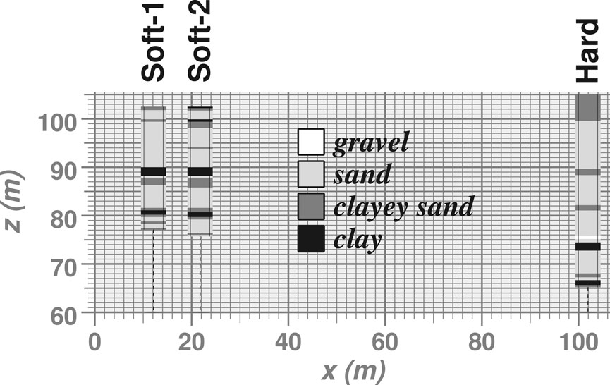
FIGURE 1. Lithologic data within a geologic cross-section, Savannah River Site, South Carolina. Data labeled “Soft-1” and “Soft-2″ are inferred from resistivity logs, and data marked “Hard” are obtained from core descriptions.

The lithologic data for two boreholes in the vicinity of the cross-section were used to calculate matrices of transition probability measurements with dependence on vertical lag shown by circles in Figure 2. The transition probability measurements associated with the gravel category are somewhat erratic because of the very low proportion of gravel. As a practical matter, this sort of measurement variability caused by data sparseness should not be unduly fitted in the transition probability modeling process. A Markov chain model, shown by the solid lines in Figure 2, was fitted the calculated vertical transition probabilities through use of a matrix exponential function

$\mathbf{T}\left(h_z\right)=\text{exp}{\mathbf{R}}_z{h}_z=\text{exp}\left[\begin{array}{cccc}-2.233& 2.205& 0.028& 0.000\\ 0.013& -0.256& 0.105& 0.138\\ 0.018& 0.571& -0.952& 0.362\\ 0.000& 0.846& 0.692& -1.538\end{array}\right]h_z(21)$

where the rate coefficients in ${\mathbf{R}}_z$ are given in units of m⁻¹. As shown by Agterberg (1974) and Carle and Fogg (1997), the entries in $\mathbf{T}\left(h_z\right)$ for Eq. 21 are computed by an eigenvalue decomposition, so that each entry, $t_{jk}\left(h_z\right)$, is a weighted sum of the k (column) category proportion and three exponential functions:

$\begin{array}{c}\mathbf{T}\left(h_z\right)=\left[\begin{array}{cccc}0.006& 0.735& 0.156& 0.103\\ 0.006& 0.735& 0.156& 0.103\\ 0.006& 0.735& 0.156& 0.103\\ 0.006& 0.735& 0.156& 0.103\end{array}\right]\\ +\left[\begin{array}{cccc}0.9832& -1.1807& -0.0662& 0.2637\\ -0.0072& 0.0086& 0.0048& -0.0019\\ -0.0180& 0.0216& 0.0012& -0.0048\\ 0.0260& -0.0313& -0.0018& 0.0070\end{array}\right]\text{exp}\left[-2.250{\text{m}}^{-1}{h}_z\right]\\ +\left[\begin{array}{cccc}0.0117& 0.0573& 0.2117& -0.2807\\ 0.0019& 0.0095& 0.0351& -0.0465\\ 0.0116& 0.0568& 0.2100& -0.2784\\ -0.0321& -0.1568& -0.5800& 0.7688\end{array}\right]\text{exp}\left[-1.840{\text{m}}^{-1}{h}_z\right]\\ +\left[\begin{array}{cccc}-0.0004& 0.3881& -0.3018& -0.0860\\ -0.0003& 0.2466& -0.1917& -0.0546\\ 0.0008& -0.8137& 0.6326& 0.1802\\ 0.0006& -0.5472& 0.4255& 0.1212\end{array}\right]\text{exp}\left[-0.890{\text{m}}^{-1}{h}_z\right]\end{array}$

For the lateral x direction, Markov chain transition probability models were developed for the SRS example based on prior geological estimates of lithofacies mean lengths and juxtapositional tendencies indicated by geologic cross-sections. Such geological information can be converted into lateral transition rates (e.g., ${\mathbf{R}}_x$) to enable development of 2- and 3-D Markov chain models and demonstrated by Carle and Fogg (1997), Carle et al. (1998), and Weissmann et al. (1999).

FIGURE 2

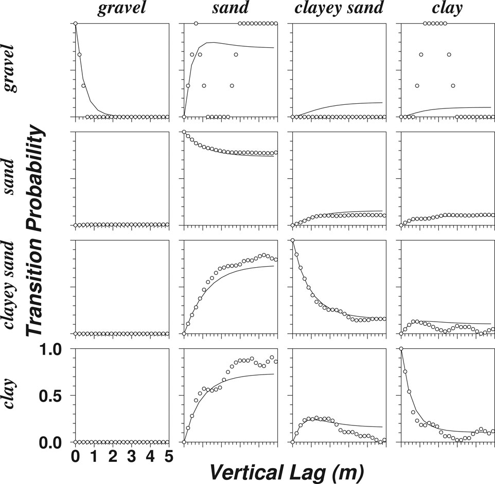
FIGURE 2. Vertical direction transition probability measurements (circles) and Markov chain model (lines).

3.2 Geostatistical Simulation with Soft Data at SRS

3.2.1 Effect of Soft Data

Figure 3 compares (A) six realizations generated with hard data only with (B) six realizations generated with hard and soft data. In (A) and (B), the hard data are honored on the right side of each realization where the solid vertical line is shown. In (B), the soft data are added as conditioning with hardness = 0.80 at the locations shown by dashed vertical lines toward the left side of each realization. With careful examination near soft data locations, the soft data impart a strong yet inexact influence on the lithofacies occurrences. For example, the occurrences of clay between about z = 87–90 m in both soft data boreholes produces a persistent clay layer in all six realizations, although the fit to the soft data values is not always exact. Near the top of the soft data shown in Figure 1 at z = 98–102.5 m, more clay and clayey sand is indicated on the right. The realizations in Figure 3 honor these data, but to a lesser extent than between z = 87–90 m where lateral correlation of the soft data is stronger. This comparison is a simple example of how tsim-s can be used to further constrain the realizations with soft data as compared to conditioning with only hard data, as could otherwise be implemented with tsim.

FIGURE 3

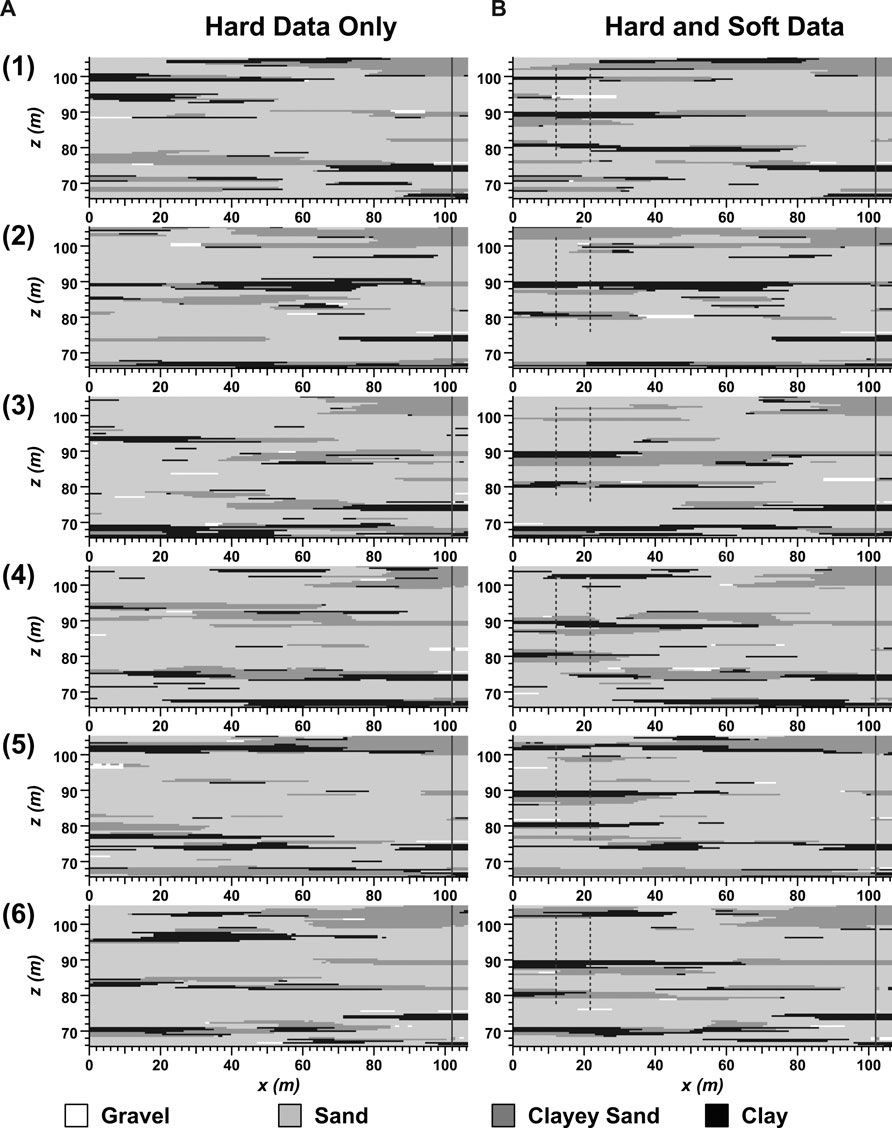
FIGURE 3. Six lithofacies realizations generated for cases with (A) hard data only and (B) hard and soft data. Hard data locations are indicated by solid line at right, and soft data locations are indicated by dashed lines at left in (B).

Another way to visualize the impact of the soft data is to average the indicator values over many realizations to produce a “probability map” for each lithofacies. Figure 4 shows probability maps for each lithofacies derived from 100 realizations with and without soft data conditioning. In case (A) with hard data only, the lithofacies probabilities approach marginal probabilities (proportions) toward the left portion of the realizations. In case (B) with hard and soft data, the soft data further constrain the probability structure toward the left side of the realizations. However, less-refined “gray areas” remain between the borehole data because of the limited lateral correlation of the lithofacies units. Overall, the soft conditioning at 0.80 hardness imparts a strong influence on the realizations.

FIGURE 4

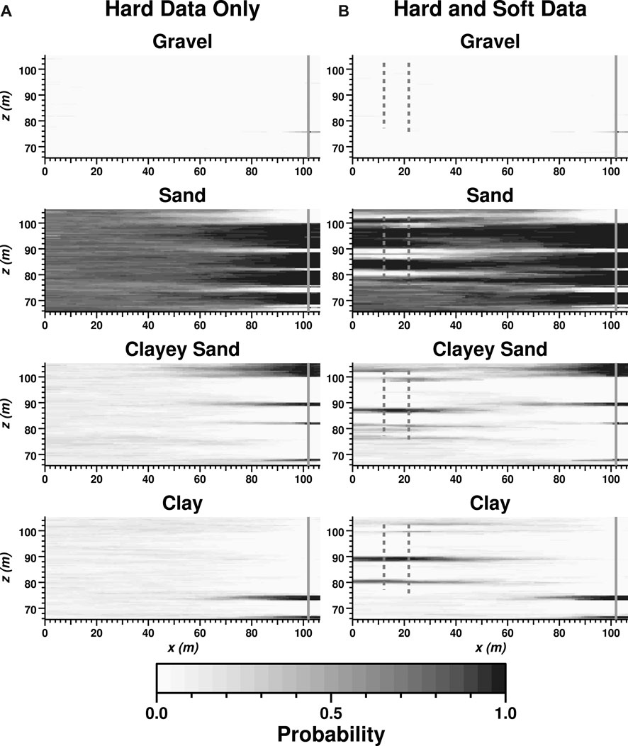
FIGURE 4. Maps of probability of occurrence for each lithofacies, based on mean indicator value of 100 realizations, for cases with (A) hard data only and (B) hard and soft data (soft data hardness = 0.8).

Through the hardness parameter, the degree of influence by the soft data can be controlled as needed in application of tsim-s. Figure 5 shows probability maps for the sand, clayey sand, and clay lithofacies where hardness values for the soft data are reduced to 0.5 and 0.2. Reducing the hardness produces less contrast or more gray areas in the probability map, which reflects the increased uncertainty of the soft data.

FIGURE 5

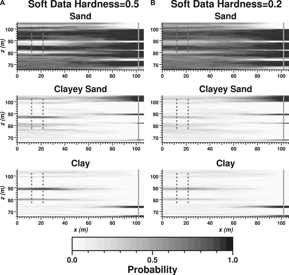
FIGURE 5. Maps of probability of occurrence for sand, clayey sand, and clay lithofacies, based on mean indicator value of 100 realizations, for cases of hard and soft data with (A) soft data hardness = 0.5, and (B) soft data hardness = 0.2.

3.2.2 Use of Realizations as Soft Conditioning

There is increasing interest in use of stochastic inversion approaches to modify heterogeneity structures within geostatistical realizations to be more consistent with geophysical or hydraulic testing data (Aines et al., 2002; Harp et al., 2008; Wainwright et al., 2014; Berg and Illman, 2015; Wang et al., 2017). To implement these approaches, there can be a need to modify an initial heterogeneity structure in a controlled or incremental manner.

Another application of the soft data capability in tsim-s is to use all or part of a realization as soft conditioning to exert control on the modification of heterogeneity structures from one realization to the next. One realization (or any available field of categorical values) can be used as prior information for conditioning of a new realization, which makes several new capabilities available in tsim-s:

• The degree of correlation between a series of realizations or can be controlled.

• The degree of variation from one realization to the next can be controlled at different locations within each realization.

• By exerting control on the difference between one realization and the next, Monte Carlo Markov chain algorithms can be implemented as a Bayesian inverse approach to optimization of local heterogeneity structure (Aines et al., 2002; Wainwright et al., 2014; Wang et al., 2017).

In practice, we refer to a realization used for soft conditioning as the “prior realization” and a subsequent realization that is produced as the “posterior realization.” Use of prior realizations as soft conditioning in the SIS step is implemented by adding only one additional soft datum to each cokriging estimate Eq. 6; that additional soft datum consists of the indicator values from the grid cell of the prior realization corresponding to the cokriging estimation location for the posterior realization. More soft data can be used, but one prior realization soft datum at the cokriging estimation location itself provides sufficient conditioning for generating correlated realizations without adding much more computational burden. The degree of correlation between the prior and posterior realizations is controlled by setting the hardness values, which may vary with location.

Figure 6 shows a sequence of six realizations where each posterior realization is soft-conditioned to the prior realization for cases of (A) hardness = 0.5 and (B) hardness = 0.9. Because the degree of hardness controls the degree of similarity (or rate of change) between one realization and the next, the realizations in case (A) are less similar (or more different) from one realization to the next. Comparing the left side (away from the hard conditioning) of realizations 1 and 6, similarities have largely disappeared for case (A) but remain for case (B). Thus, the higher rate of change (lesser hardness) shortens the memory of heterogeneity patterns within a sequence of realizations soft-conditioned by prior realizations.

FIGURE 6

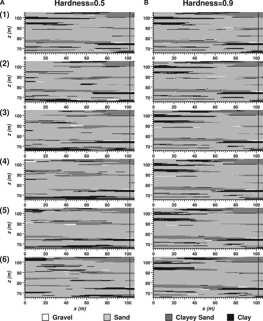
FIGURE 6. Six successive realizations where the previous realization serves as soft conditioning, with hardness set for case (A) at 0.5 and case (B) at 0.9.

Figure 7 shows an example using the same realization as soft data (upper left) with hardness varying with depth from 0.8 at top to 0.0 at bottom. The probability maps for gravel, sand, clayey sand, and clay facies, derived from 100 realizations generated by tsim-s, show increasing uncertainty with depth. In particular, the location of individual clayey sand and clay lenses in the soft data become less distinct with depth in the probability maps. Likewise, the sand probabilities become less distinct with depth and approach the proportion of 0.735. The influence of a single gravel lens in the soft data is evident in the gravel probability map. This example illustrates how 2or 3-D geophysical images or geological interpretations of categorical data might be used to soft-condition geostatistical realizations with consideration of variable spatial resolution such as decreasing resolution with increasing depth.

FIGURE 7

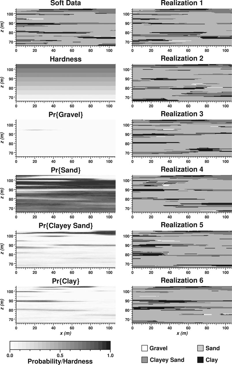
FIGURE 7. Example using a realization as soft data (upper left) with hardness varying with depth (left, second from top). Probability maps for gravel, sand, clayey sand, and clay facies (lower left) are derived from 100 realizations. The first six soft-conditioned realizations are shown at right.

3.3 Application to Large-Scale Simulation

3.3.1 Computational Aspects

Like tsim, tsim-s is readily extended to large-scale three-dimensional (3-D) applications. From a computational standpoint, the main difference between running tsim and tsim-s will be in memory use. For very large grid cell counts (tens of millions or more), the memory use in tsim is mostly taken up by integer arrays storing the grid cell category and anisotropy direction information (if used). In the late 1990s when memory was quite restricted compared to the year 2020, a 45-million cell 3-D realization was produced on a computer with 48 megabytes (not gigabytes!) of memory by modifying tsim to use a 1-byte integer format for the grid cell array and implementing an analytical function to define variable stratigraphic directions (Carle, 1996; Carle et al., 1998; Carle, 1999; Tompson et al., 1999). The open-source nature of the T-ProGS package of codes enables the user to make similar modifications to conserve memory. Depending on the application, tsim-s will require a factor of as much as ten or more times the memory use as tsim, but computational time tsim-s will not be significantly higher because the corresponding arrays for the cokriging equations and quenching objective function are of the same dimensions under similar model parameter settings. Considering that computer memory and computational speed are orders of magnitude higher today and into the future as compared to the late 1990s, we do not anticipate large-scale simulation of categorical heterogeneity with tsim-s to be highly constrained by the current or future computational technology.

3.3.2 Llagas Basin Example

As discussed in the introduction, the use of driller’s logs in categorical geostatistical simulation is of interest in hydrogeology, yet presents some uncertainty in how to treat driller’s logs as conditioning data. As a demonstration of the use of driller’s logs and tsim-s to large-scale simulation, Figure 8A shows an interpreted version of a driller’s log dataset, and Figure 8B shows a 3-D simulation of hydrostratigraphic architecture for the Llagas groundwater subbasin south of San Jose, California (Carle et al., 2004; Carle et al., 2006).

FIGURE 8

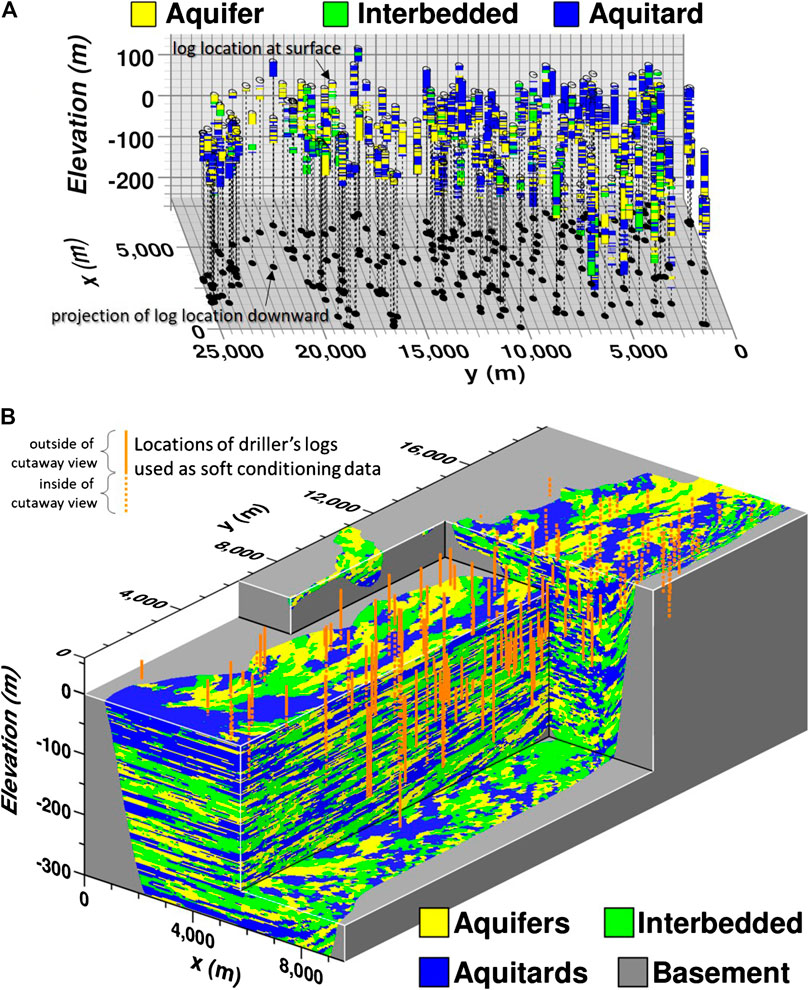
FIGURE 8. (A) Hydrofacies interpretations of driller logs and (B) example 3-D simulation of aquifer system heterogeneity using tsim-s showing locations of conditioning data and variable dip and flow directions of anisotropy. Modified from Carle et al. (2006).

In this application, the driller’s log data were categorized into aquifer, interbedded, and aquitard hydrofacies, where the interbedded category represents relatively thin interlayers of aquifer and aquitard materials. The addition of the interbedded hydrofacies addresses unresolvable fine-scale heterogeneity of coarse- and fine-grained textural classifications and adds flexibility to development of the Markov chain model. If only two hydrofacies, aquifer and aquitard, had been distinguished, the 3-D Markov chain model would consist of only four parameters - proportion and mean length in the three principal depositional directions for one of the hydrofacies; the remaining transition probabilities are all determined by probability law (Carle and Fogg, 1996). A two-category characterization of heterogeneity presents no distinct advantage in the Markov chain spatial variability modeling framework; the spatial variability model is equivalent to a two-category indicator variogram-based approach modeled by an exponential variogram. With three categories, the number of parameters for the 3-D Markov chain is raised to 14, allowing for development of more complexity in the heterogeneity structure including asymmetry such as fining-upward and outward tendencies (Miall, 1973; Carle and Fogg, 1997; Fogg et al., 1998).

This simulation was generated by tsim-s with soft conditioning data divided into three sets of driller’s logs to which hardness levels were set to 0.3, 0.7, and 1.0 based on data quality. Two separate tsim-s simulations of 162,500,000 and 117,000,000 cells were generated for the upper and lower portions of the final realization of hydrofacies architecture to address differences in the spatial structure of deeper and shallower alluvial hydrofacies evident in the driller’s logs. Carle et al. (2006) provides further detail on the process of selection of the hardness parameter in the practical hydrogeological situation of using driller’s logs for conditioning data. This example confirms that large-scale 3-D stochastic simulation using tsim-s is feasible. The stochastic analysis was further applied to investigate permeability heterogeneity effects on nitrate transport from agricultural sources toward municipal wells (Carle et al., 2004, Carle et al., 2006).

4 Discussion

The discussion focuses on capabilities and limitations of t-sim and tsim-s with attention to the current literature on comparison and evaluation of geostatistical methods for subsurface characterization of categorical variables.

4.1 Curvilinear Features

Both tsim and tsim-s have the capability to produce curvilinear features by specifying azimuthal and dip angles local to each grid cell in an a priori manner (Carle, 1999; Carle, 2007) that can be deterministic (Tompson et al., 1999; Carle et al., 2006) or stochastic (Carle et al., 1998). These angles may be derived or inferred from prior geological knowledge or geologically reasonable interpretation of the depositional or stratigraphic architecture, surface mapping of the deep soil horizons, interpretation of seismic or surface geophysical data, or stochastic modeling (e.g., by modeling variation in the major axis of deposition due to meandering by a gaussian random field). Local anisotropy directions are implemented in tsim and tsim-s in a manner similar to “local anistropy kriging” (te Stroet and Snepvangers, 2005). This is not a coordinate transformation approach, as applied to the variogram-based isim3D (Gomez-Hernandez and Srivastava, 1990).

The Llagas basin example application of tsim-s uses the local anisotropy direction option to impart variable angles of dip and principle direction of deposition into the geostatistical realizations. Figure 9 shows vertical and horizontal slices through the 3-D Llagas basin realization to better reveal the nature of the curvilinear features. These include variable dip angles evident in longitudinal and transverse-plane cross-sections (A) and (B) and variable direction in the major axis of deposition in the horizontal-plane cross-section (C).

FIGURE 9

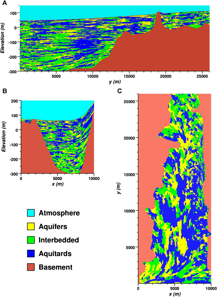
FIGURE 9. Cross-section through the 3-D simulation shown in Figure 8 throught (A) longitudinal (B) lateral, and (C) horizontal planes.

The simulated aquifer/interbedded facies architecture for the Llagas basin example does not show pronounced sinuousity, which is consistent with how channel belt deposits were conceptualized in this alluvial depositional setting by the California Department of Water Resources (1981). This is in contrast to the “true” or “training image” concept of continuous “channels” worming their way through homogeneous low-pemeability media, a common argument posed for replacing bivariate statistical methods with multi-point statistical (mps) methods (Strebelle, 2000; Caers, 2001; Krishnan and Journel, 2003; Feyen and Caers, 2006; Ronayne et al., 2008; Li et al., 2014a; Li et al., 2015; Mariethoz and Caers, 2015; Zovi et al., 2017; Ramgraber et al., 2020). Such surficially-based conceptual models gloss over fundamental geologic concepts showing how depositional processes produce amalgamations of channel and adjacent sediments that are broader, less sinuous, and more variable in lateral extent as compared to an active fluvial channel viewed on the Earth’s surface (Galloway and Hobday, 1996; Miall, 2013). It is a well-known fact in interpretation of borehole data that sedimentary features on the surface are not necessarily preserved in the subsurface (Smith, 2002).

4.2 Methods Comparison

The T-ProGS software package has been used somewhat frequently for comparison of methods for geostatistical simulation of categorical variables (Carle, 1996; Carle, 2000; Lee et al., 2007; Yong et al., 2009; Bianchi et al., 2011; dell’Arciprete et al., 2012; Ranjineh Khojasteh, 2013; Kessler et al., 2013; Guastaldi et al., 2014; Serrano et al., 2014; Hoyer et al., 2015; Damico et al., 2018). Bianchi et al. (2011) and Ranjineh Khojasteh (2013) present rigorous comparisons of tsim and sisim, showing that sisim does not honor the 3-D model of spatial variability, which was one of the original motivations for developing T-ProGS (Carle, 1996; Carle, 1999; Carle, 2000).

We further discuss methods comparison below because tsim-s carries forward several capabilities of tsim that appear not to be recognized in the methods comparison literature. Flawed methods comparison causes a trickle-down effect of selective references that propogate misleading appraisals of the capabilities of the available methods for stochastic simulation of categorical variables.

In a methods comparsion of sisim, tsim, and mps, dell’Arciprete et al. (2012) did not consider variable anistropy directions in either conceptualization or parameterization of their analysis of spatial variablity and applications of tsim despite obvious dipping structures in their data. They chose not to apply Markov chain modeling concepts in the structural framework of a stratigraphic coordinate system relevant to the hydrofacies of a sedimentary depositional system (Carle et al., 1998; Tompson et al., 1999; Carle et al., 2006). The example of a tsim realization shown in Figure 4 of dell’Arciprete et al. (2012) displays completely random-looking and geologically implausible spatial structuring inconsistent with the data and geologic setting.

An example of a trickle-down effect is how dell’Arcipreti et al. (2012) becomes a main reference in He et al. (2017) for promoting application of mps, then (He et al., 2017) becomes a main reference in Langousis et al. (2018) for criticizing the 3-D Markov chain modeling approach of Carle and Fogg (1997). To “reveal” limitations of Markov chain models, Langousis et al. (2018) execute a “simple test-case” of a 2-D dipping layer with a coordinate system anchored in the vertical and horizontal directions of their statistical analysis. Neither dell’Arciprete et al. (2012) nor Langousis et al. (2018) appeared to grasp the concept that bivariate geostatistical analysis and simulation should be applied in a geologically-based coordinate system, as demonstrated for at least 30 years (e.g., Gomez-Hernandez and Srivastava, 1990). The geological realism of the mps application by He et al. (2017) stands wide open to geological criticism too, with a mps-generated “real world buried valley system” showing unrealistic topography and isolated occurrences of the valley fill buried beneath pre-valley-fill strata. Geostatistical analysis should recognize and make adjustments to account for geological slopes, directions, and depositional ordering and not be strictly anchored in a rectilinear cooordinate system pertinent only to data locations.

Another pitfall of methods comparison is use of oversimplified example applications. In Kessler et al. (2013), tsim was compared to mps in application to stochastic simulation of sand lenses within clayey till. This application of tsim adhered to an oversimplified two-category Markov chain to model “a complex type of heterogeneity” exhibiting a bi-modal distribution in the size of sand lenses in 2-D training and reference images. A simple way to address this facies size distribution complexity would be to define two types of sand lenses (perhaps “small” and “large”) and model a three-category system. Instead of adhering to a textural basis for defining categories (e.g., “sand” and “clay”), a more geological approach is to interpret hydrofacies appropriate to the geometric framework of the depositional system (Fogg et al., 1998).

The impact of methods comparison studies can get more convoluted by selective referencing of the literature, particularly on the topic of curvilinear features. For example, in promoting mps, Barfod et al. (2018) dissmiss applicability of tsim by stating that “…T-ProGS also has difficulties in reconstructing curvilinear geological features” without any reference to previous work in which the variable anisotropy direction capability of tsim was implemented. Barfod et al. (2018) refer to the oversimplified two-category sand-clay Markov chain analysis of Kessler et al. (2013) as “revealing a sub-optimal pattern reproduction, in comparison to other simulation tools such as multiple-point statistics…” Linde et al. (2015) in reviewing “variogram based models” state that “transition probability techniques such as T-ProGS … cannot properly produce curvilinear features…” This is after referencing only dell’Arciprete et al. (2012), Falivene et al. (2007), Lee et al. (2007), and Reffsgaard et al., 2014) as T-ProGS applications, all four of which did not employ variable anisotropy direction capability in tsim. The misconception that all bivariate statistical methods for stochastic simulation of categorical variables lack the ability to produce curvilinear features appears to derive from selective referencing and comparison of mps to only variogram-based methods (Strebelle, 2002; Caers, 2001; Krishnan and Journel, 2003; Feyen and Caers, 2006; Linde et al., 2015; Barfod et al., 2018) irrespective of previous hydrogeologic studies (Carle et al., 1998; Tompson et al., 1999; Carle et al., 2006; Green et al., 2010; Engdahl et al., 2012) and the T-ProGS user manual (Carle, 1999; Carle, 2007).

If tsim or tsim-s is producing spatial structure that falls well short of the intended model for represention of the spatial heterogeneity, the conceptualization, implementation, or utilization of the capabilities of tsim or tsim-s may be at fault. Methods comparison studies in geostatistics should fully investigate the capabilities of each method including both the geological and statistical conceptual underpinnings before making sweeping judgments. The introduction of this paper provides references to varied applications of T-ProGS that should be useful for methods comparison and capabilities assessment.

4.3 Method Limitations

All models have limitations. The T-ProGS package was originally conceived in 1996 (Carle, 1996; Carle, 1997; Carle and Fogg, 1996; Carle and Fogg, 1997) to improve or add to the capabilities of the then state-of-the art variogram-based geostatistical methods of the Geostatistical Software Library (Deutsch and Journel, 1992) and subsequently analyze pumping test data in a highly heterogeneous alluvial aquifer system (Carle, 1996; Lee et al., 2007). It is easy to argue that natural systems are geometrically inconsistent with certain geostatistical representations or exhibit far more complexity than any bivariate geostatistical model could ever characterize. Different practitioners will be more comfortable with different methods or levels of complexity in the statistical or bio/chemo/hydrogeological components of their models. There will always be an open question as to what levels of complexity are necessary to sufficiently analyze the subsurface processes of interest.

The stationarity assumption in regard to the spatial continuity model and category proportions can be limiting. Early applications of tsim recognized this issue and incorporated “nonstationary” qualities into the geostatistics through data conditioning, geologically-based zones based on stratigraphic analysis or sedimentary environments, and spatially variable angles of anistropy (Carle, 1996; Carle, 2000; Carle et al., 1998; Tompson et al., 1999; Weissmann and Fogg, 1999). There continue to be applications of tsim that recognize and address nonstationarity (Weissmann et al., 2004; Traum et al., 2014; Weissmann et al., 2015; Meirovitz et al., 2017; Zhu et al., 2016a; Zhu et al., 2016b; Zhang et al., 2018; Liao et al., 2020; Maples et al., 2020). As discussed previously for application of tsim-s, Carle et al. (2006) employed two-zones of differing spatial statistics and apply variable anisotropy directions in their application of tsim-s. To address geological realism, adding a modicum of geological insight can be more effective than adding more statistical complexity.

The model of spatial variability is another limitation to any geostatistical approach. A methods limitations analysis by Langousis et al. (2018) criticizes the interpretive framework of transition probability-based Markov chain model development as “based on unverified/untested simplifying assumptions” and “ad-hoc manipulations.” Langousis et al. (2018) further contend that.

…stochastic modeling of actual geologies using the [T-ProGS] approach of Carle and Fogg (1997), is characterized by simplifying assumptions and theoretical limitations, with the simulated random fields exhibiting statistical structures that strongly depend on the problem under consideration and the modeling assumptions made, leading to increased epistemic uncertainties in the obtained results.

We offer some perspectives on assessing the limitations of T-ProGS that apply to tsim-s as well:

• Use of geological concepts in categorical geostatistical simulation may involve subjectivity, which can be viewed by some as either a strength or a limitation to reducing uncertainty.

• The implication that injection of subjective geologic interpretation increases epistemic uncertainties in stochastic modeling would appear to expose a lack of understanding of subsurface geology and it’s role in modeling the subsurface.

• As referenced in the introduction of this paper, many applications in hydrogeology and related fields have found the Markov chain modeling framework to be useful to characterization of bivariate spatial statistical cross-relationships (i.e., juxtapositional tendencies), which can be related in an interpretive manner to geological concepts such as Walther’s Law in the stratigraphic context of sedimentary depositional environments (Leeder, 1982; Doveton, 1994).

• As evident in the T-ProGS manual (Carle, 1999; Carle, 2007), the Markov chain is not actually required to run tsim (or tsim-s). So one could investigate epistemic aspects of other transition probability or indicator covariance models using tsim, tsim-s, or the various variogram-based simulation methods, if so desired. However, such methods comparison exercises, which can certainly be expanded to all stochastic models, will not prove that a spatial Markov chain is not useful to modeling subsurface hydrofacies heterogeneity when applied in the appropriate geologic context.

In every subsurface heterogeneity modeling project we have encountered, the heterogeneity contains both deterministic and stochastic aspects that should be treated differently. For example, conventional geologic stratigraphic analysis is quite effective for identifying and mapping the major formations, depositional systems, and the bounding unconformities and structural discontinuities (e.g., faults). Accordingly, such features can typically be treated deterministically and then used as the basis for appropriate geologic zoning of the system into quasi-stationary subdomains. The stochastic aspect of subsurface characterization typically lies within those geologically defined subdomains. If one, however, lumps together both the deterministic and stochastic aspects of the heterogeneity and calls on the stochastic geostatistical algorithm to sort out those spatial patterns, one only invites naive mischaracterization of the heterogeneity that produces unnecessary uncertainty and unrealistic results. An effective way to reduce or moderate uncertainty is to recognize and separate out deterministic and stochastic parts of the problem.

4.4 Stochastic Methods Evaluation

Stochastic methods evaluation in hydrogeology should strive to determine appropriate levels of complexity necessary for gaining insight to 3-D subsurface flow and transport processes at scales relevant to measurement diagnostics used in decision-making. An example of a process-oriented methods comparison, Damico et al. (2018) compared dynamics and trapping metrics for 3-D carbon-dioxide plume simulations using subsurface representations of heterogeneity derived from tsim and a more rigorous model for representation of complex features in fluvial architecture. They concluded:

…in the context of representing plume dynamics and residual trapping within fluvial deposits, and within the scope of the parameters used here, the simpler geostatistical model of braided fluvial deposits appears to give an adequate representation of the smaller scale heterogeneity. The depositional- and geometric-based benchmark models represented more features of the fluvial architecture, including variability in the dip of cross sets, variability in the geometry and orientation of unit bars, and the occurrence of channel fills. Depending on context, representing those features may be quite important to understanding some multiphase flow processes in aquifers and reservoirs. However, the simpler geostatistical model (tsim) is able to capture the important aspects of fluvial architecture within the context of understanding the general effect of smaller scale heterogeneity on residual trapping of CO₂ in geosequestration reservoirs, within the scope of the parameters used here.

The worthiness of a stochastic methods to subsurface applications does not necessarily depend on statistical rigor or geological detail, it also depends on the perception of relative value, including both benefits and costs, in the application (Ginn, 2004). The relative value of a model is not necessarily in its complexity, given that calibration of more complex models may erode rather than enhance predictive ability (Doherty and Christensen, 2011).

This paper is offering an approach to address uncertainty in data conditioning of categorical geostatistical models. It would be quite straightforward to add more statistical complexity to transition probability or hardness concepts. However, in our nearly 25-year experience with using transition probability-based geostatistics, we find simpler and more interpretetable geologically-based tools to be quite useful in the study of the effects of various scales and types of heterogeneity on subsurface flow and transport processes.

5 Conclusions

Many Earth science applications would benefit from increased ability to incorporate “soft” (uncertain or indirect) data to further constrain subsurface models of heterogeneity. In categorical geostatistical simulation applications, often abundant soft data on lithology or hydrofacies (e.g., geophysical logs and imaging, geological interpretations, driller’s logs, etc.) offer opportunity for imposing increased or relaxed model constraint.

A soft data capability has been incorporated into the categorical geostatistical simulation code tsim-s. Soft data for categorical variables are input either as indicator values or prior probabilities, and a “hardness” value accounts for uncertainty in the data. This approach is particularly conducive to soft data that is already categorical, such as texture inferred from driller’s logs, hydrofacies interpretations, or electrofacies based on resistivity cutoffs. In generating realizations with tsim-s, the impact of uncertainty in the soft data is factored into formulation of both the cokriging and simulated quenching geostatistical simulation steps. The extent to which the realizations honor the soft data is balanced by the values of hardness, the model of spatial variability, and the values of other nearby hard and soft data.

The degree to which soft data reduces variability in simulation outputs can be quantified by mapping facies probabilities derived by averaging indicator values from many realizations. Example applications in this paper using different values and spatial distributions of hardness illustrate how the impact of data uncertainty can be controlled in the stochastic realizations. Such control will be useful for assimilating different data sets of variable resolution and accuracy. The soft conditioning can be arrays of data, including “prior realizations,” to incrementally adjust or evolve the spatial heterogeneity structure of the realizations. The ability to manipulate localized heterogeneity structure or rate of change in a sequence of realizations should be useful for flow and transport model calibration, inverse approaches, or sensitivity analysis. The tsim-s algorithm is ammenable to large-scale 3-D simulation including curvilinear features.

Overall, the tsim-s code more rigorously integrates data uncertainty and prior information into the categorical stochastic simulation algorithm as compared to previous indicator-based geostatistical simulation codes including its direct predecessor tsim. However, users and evaluators of bivariate geostatistical models should become familiarized with capabilities, limitations, and varied uses of T-ProGS or other geostatistical software packages before applying or evaluating tsim or tsim-s.

Data Availability Statement

The data analyzed in this study is subject to the following licenses/restrictions: must be obtained by permission. Requests to access these datasets should be directed to carle1@llnl.gov.

Author Contributions

SC developed code, executed applications, and wrote first draft of article. GF aided in theoretical development, outside application, tie-in to other research, and assisted SC in revision of the manuscript.

Conflict of Interest

The authors declare that the research was conducted in the absence of any commercial or financial relationships that could be construed as a potential conflict of interest.

Acknowledgments

The authors thank Roger Aines, John Nitao, and Abe Ramirez at the Lawrence Livermore National Laboratory for their input and support toward developing tsim-s, Rolf Aadland and other SRS staff for supplying data and hydrogeological cross-sections, and Yong Zhang at University of California Davis for a preliminary geostatistical analysis of the SRS data. This work was performed under the auspices of the U.S. Department of Energy by Lawrence Livermore National Laboratory under Contract No. DE-AC52-07NA27344.

References

Aadland, R. K., Gellici, J. A., and Thayer, P. A. (1995). “Hydrogeologic framework of west-central South Carolina,” in Water resources division report. Columbia, US: South Carolina Department of Water Resources, Vol. 5.

Google Scholar

Aarts, E., and Korst, J. (1989). Simulated annealing and Boltzmann machines. New York, NY: John Wiley and Sons.

Google Scholar

Abriola, L. M., Cápiro, N. L., Christ, J. A., Chu, L., Miller, E. L., and Pennell, K. D. (2019). Final report, project ER-2311. Alexandria, VA: Strategic Environmental Research and Development Program.

Google Scholar

Agterberg, F. P. (1974). Geomathematics. Amsterdam, NY: Elsevier Scientific Publishing Company.

Google Scholar

Aines, R., Nitao, J., Newmark, R., Carle, S., Ramirez, A., Harris, D., et al. (2002). UCRL-ID-148221. The stochastic engine initiative: improving prediction of behavior in geologic environments we cannot directly observe. Livermore, CA: Lawrence Livermore National Laboratory.

Google Scholar

Alberto, M. C. (2010). Heterogeneidades geológicas e o gerenciamento de áreas contaminadas em local situado na Interface da Serra do Mar com a Planície Aluvionar do Rio Cubatão (Cubatão/SP). Tese (doutorado). Brazil: Universidade Estadual Paulista, Instituto de Geocióncias e Cióncias Exatas.

Google Scholar

Amooie, M. A., Soltanian, M. R., Xiong, F., Dai, Z., and Moortgat, J. (2017). Mixing and spreading of multiphase fluids in heterogeneous bimodal porous media. Geomech. Geophys. Geo-energ. Geo-resour. 3 (3), 225–244. doi:10.1007/s40948-017-0060-8

CrossRef Full Text | Google Scholar

Arihood, L. D. (2009). Processing, analysis, and general evaluation of well-driller records for estimating hydrogeologic parameters of the glacial sediments in a ground-water flow model of the Lake Michigan Basin. Scientific Investigations Report 2008-5184. Reston, VA: US Geological Survey, 26.

Google Scholar

Arshadi, M., De Paolis Kaluza, M. C., Miller, E. L., and Abriola, L. M. (2020). Subsurface source zone characterization and uncertainty quantification using discriminative random fields. Water Resour. Res. 56 (3), e2019WR026481. doi:10.1029/2019wr026481

CrossRef Full Text | Google Scholar

Back, P. E., and Sundberg, J. (2007). Thermal site descriptive model. A strategy for the model development during site investigations-version 2 (No. SKB-R–07-42). Stockholm, SE: Swedish Nuclear Fuel and Waste Management Co., 1402–3091.

Google Scholar

Baidariko, E. A., and Pozdniakov, S. P. (2011). Simulation of liquid waste buoyancy in a deep heterogeneous aquifer. Water Resour. 38 (7), 972–981. doi:10.1134/s0097807811070037

CrossRef Full Text | Google Scholar

Bakshevskaia, V. A., and Pozdniakov, S. P. (2016). Simulation of hydraulic heterogeneity and upscaling permeability and dispersivity in sandy-clay formations. Math. Geosci. 48 (1), 45–64. doi:10.1007/s11004-015-9590-1

CrossRef Full Text | Google Scholar

Barfod, A. S., Moller, I., Christiansen, A. V., Hoyer, A. S., Hoffimann, J., Straubhaar, J., et al. (2018). Hydrostratigraphic modeling using multiple-point geostatistics and airborne transient electromagnetic methods. Hydrol. Earth Syst. Sci. 22, 3351–3373. doi:10.5194/hess-22-3351-2018

CrossRef Full Text | Google Scholar

Beisman, J. J., Maxwell, R. M., Navarre-Sitchler, A. K., Steefel, C. I., and Molins, S. (2015). ParCrunchFlow: an efficient, parallel reactive transport simulation tool for physically and chemically heterogeneous saturated subsurface environments. Comput. Geosci. 19 (2), 403–422. doi:10.1007/s10596-015-9475-x

CrossRef Full Text | Google Scholar

Berg, S. J., and Illman, W. A. (2015). Comparison of hydraulic tomography with traditional methods at a highly heterogeneous site. Groundwater. 53 (1), 71–89. doi:10.1111/gwat.12159

CrossRef Full Text | Google Scholar

Berretta, G. P., and Felletti, F. (2007). Previsione della presenza di massi nello scavo di gallerie in depositi glaciali: approccio geostatistico mediante T-ProGS (transition probability geostatistics). Geoing. Ambient. e Mineraria. 2, 5–21. doi:10.1016/j.enggeo.2009.06.006

Google Scholar

Bianchi, M. (2017). Validity of flowmeter data in heterogeneous alluvial aquifers. Adv. Water Resour. 102, 29–44. doi:10.1016/j.advwatres.2017.01.003

CrossRef Full Text | Google Scholar

Bianchi, M., Kearsey, T., and Kingdon, A. (2015). Integrating deterministic lithostratigraphic models in stochastic realizations of subsurface heterogeneity. Impact on predictions of lithology, hydraulic heads and groundwater fluxes. J. Hydrol. 531 (3), 557–573. doi:10.1016/j.jhydrol.2015.10.072

CrossRef Full Text | Google Scholar

Bianchi, M., and Pedretti, D. (2017). Geological entropy and solute transport in heterogeneous porous media. Water Resour. Res. 53 (6), 4691–4708. doi:10.1002/2016wr020195

CrossRef Full Text | Google Scholar

Bianchi, M., Zhang, L., and Birkholzer, J. T. (2016). Combining multiple lower-fidelity models for emulating complex model responses for CCS environmental risk assessment. Int. J. Greenh. Gas Control. 46, 248–258. doi:10.1016/j.ijggc.2016.01.009

CrossRef Full Text | Google Scholar

Bianchi, M., and Zheng, C. (2016). A lithofacies approach for modeling non-Fickian solute transport in a heterogeneous alluvial aquifer. Water Resour. Res. 52 (1), 552–565. doi:10.1002/2015WR018186

CrossRef Full Text | Google Scholar

Bianchi, M., Zheng, C., Wilson, C., Tick, G. R., Liu, G., and Gorelick, S. M. (2011). Spatial connectivity in a highly heterogeneous aquifer: from cores to preferential flow paths. Water Resour. Res. 47 (5), W05524. doi:10.1029/2009WR008966

CrossRef Full Text | Google Scholar

Blessent, D. (2013). Stochastic fractured rock facies for groundwater flow modeling. Dyna. 80 (182), 88–94.

Google Scholar

Blessent, D., Barco, J., Temgoua, A. G. T., and Echeverrri-Ramirez, O. (2017). Coupled surface and subsurface flow modeling of natural hillslopes in the Aburrá Valley (Medellín, Colombia). Hydrogeol. J. 25 (2), 331–345. doi:10.1007/s10040-016-1482-z

CrossRef Full Text | Google Scholar

Blessent, D., Therrien, R., and Lemieux, J. M. (2011). Inverse modeling of hydraulic tests in fractured crystalline rock based on a transition probability geostatistical approach. Water Resour. Res. 47 (12), 88-94. doi:10.1029/2011wr011037

CrossRef Full Text | Google Scholar

Bohling, G. C., and Butler, J. J. (2010). Inherent limitations of hydraulic tomography. Groundwater. 48 (6), 809–824. doi:10.1111/j.1745-6584.2010.00757.x

CrossRef Full Text | Google Scholar

Bohling, G. C., and Dubois, M. K. (2003). An integrated application of neural network and Markov chain techniques to the prediction of lithofacies from well logs, Kansas Geological Survey Open-File Report 2003-50. Lawrence, KS: Kansas Geological Survey, 6.

Google Scholar

Boulanger, R. W., Munter, S. K., Krage, C. P., and DeJong, J. T. (2019). Liquefaction evaluation of interbedded soil deposit: Cark Canal in 1999 M7. 5 Kocaeli earthquake. J. Geotech. Geoenviron. Eng. 145 (9), 05019007. doi:10.1061/(asce)gt.1943-5606.0002089

CrossRef Full Text | Google Scholar

Burow, K. R., Jurgens, B. C., Kauffman, L. J., Phillips, S. P., Dalgish, B. A., and Shelton, J. L. (2008). Simulations of ground-water flow and particle pathline analysis in the zone of contribution of a public-supply well in Modesto, eastern San Joaquin Valley, California. Scientific Investigations Report 2008–5035. Reston, VA: US Geological Survey, 41.

Google Scholar

Burow, K. R., Weissmann, G. S., Miller, R. D., and Placzek, G. (1997). Hydrogeologic facies characterization of an alluvial fan near Fresno, California, using geophysical techniques. Open-file report. 97-46. Sacramento. CA: US Geological Survey.

Google Scholar

Buscheck, T. A., Mansoor, K., Yang, X., Wainwright, H. M., and Carroll, S. A. (2019). Downhole pressure and chemical monitoring for CO₂ and brine leak detection in aquifers above a CO₂ storage reservoir. Int. J. Greenh. Gas Con. 91, 102812. doi:10.1016/j.ijggc.2019.102812

CrossRef Full Text | Google Scholar

Caers, J., (2001). Geostatistical reservoir modelling using statistical pattern recognition. J. Petrol. Sci. Eng. 29 (3-4), 177–188. doi:10.1016/S0920-4105(01)00088-2

CrossRef Full Text | Google Scholar

California Department of Water Resources (1981). Evaluation of groundwater resources, South San Francisco Bay, volume IV, south Santa clara county area. Sacramento, CA: California Department of Water Resources Bulletin, 143.

Google Scholar

Carle, S. F. (1996). A transition probability-based approach to geostatistical characterization of hydrostratigraphic architecture. PhD dissertation. Davis (CA): University of California.

Google Scholar

Carle, S. F. (1997). Implementation schemes for avoiding artifact discontinuities in simulated annealing. Math. Geol. 29 (2), 231–244. doi:10.1007/bf02769630

CrossRef Full Text | Google Scholar

Carle, S. F. (1999). T-PROGS: transition probability geostatistical software version 2.1. Davis: University fo Caifornia Available at: http://gmsdocs.aquaveo.com/T-PROGS.pdf

Google Scholar

Carle, S. F. (2000). UCRL-JC-141551. Use of a transition probability/Markov approach to improve geostatistical simulation of facies architecture. Livermore, CA: Lawerence Livermore National Laboratory.

Google Scholar

Carle, S. F. (2003). UCRL-JC-153653. Integration of soft data into categorical geostatistical simulation. Livermore, CA: Lawrence Livermore National Laboratory.

Google Scholar

Carle, S. F. (2007). UCRL-SM-232880. T-PROGS: transition probability geostatistical software version 2.1. Livermore, CA: Lawrence Livermore National Laboratory.

Google Scholar

Carle, S. F., Esser, B. K., and Moran, J. E. (2006). High-resolution simulation of basin-scale nitrate transport considering aquifer system heterogeneity. Geosphere. 2 (4), 195–209. doi:10.1130/ges00032.1

CrossRef Full Text | Google Scholar

Carle, S. F., and Fogg, G. E. (1996). Transition probability-based indicator geostatistics. Math. Geol. 28(4), 453–476. doi:10.1007/bf02083656

CrossRef Full Text | Google Scholar

Carle, S. F., and Fogg, G. E. (1997). Modeling spatial variability with one and multidimensional continuous-lag Markov chains. Math. Geol. 29 (7), 891–918. doi:10.1023/a:1022303706942

CrossRef Full Text | Google Scholar

Carle, S. F., Labolle, E. M., Weissmann, G. S., Van Brocklin, D., and Fogg, G. E. (1998). “Geostatistical simulation of hydrofacies architecture, a transition probability/Markov approach,” in Hydrogeologic models of sedimentary aquifers, concepts in hydrogeology and environmental geology No. 1. Editors G. S. Fraser, and J. M. Davis, (Tulsa, OK: Society for Sedimentary Geology Special Publication), 147–170.

Google Scholar

Carle, S. F., and Ramirez, A. (1999). UCRL-JC-136739. Integrated subsurface characterization using facies models, geostatistics, and electrical resistance tomography. Livermore, CA: Lawrence Livermore National Laboratory.

Google Scholar

Carle, S. F., Ramiriez, A., Daily, W., Newmark, R., and Tompson, A. (1999). UCRL-JC-132943. High-perforamance computational and geostatistical experiments for testing the capabilities of 3-D electrical resistance tomography. Livermore, CA: Lawrence Livermore National Laboratory.

Google Scholar

Carle, S. F., Tompson, A. F. B., McNab, W. W., Esser, B. K., Hudson, G. B., Moran, J. E., et al. (2004). “Simulation of nitrate biogeochemistry and reactive transport in a California groundwater basin,” in Developments in water science. New York, NY: Elsevier, Vol. 55, 903–914.

Google Scholar

Carle, S. F., Zavarin, M., and Pawloski, G. A. (2002). UCRL-ID-150200. Geostatistical analysis of spatial variability of mineral abundance and Kd in Frenchman Flat, NTS, Alluvium. Livermore, CA: Lawrence Livermore National Laboratory.(Accessed November 1, 2002).

Google Scholar

Carroll, S. A., Keating, E., Mansoor, K., Dai, Z., Sun, Y., Trainor-Guitton, W., et al. (2014). Key factors for determining groundwater impacts due to leakage from geologic carbon sequestration reservoirs. Int. J. Greenh. Gas Con. 29, 153–168. doi:10.1016/j.ijggc.2014.07.007

CrossRef Full Text | Google Scholar

Chen, G., Sun, Y., Liu, J., Lu, S., Feng, L., and Chen, X. (2018). The effects of aquifer heterogeneity on the 3D numerical simulation of soil and groundwater contamination at a chlor-alkali site in China. Environ. Earth Sci. 77 (24), 797. doi:10.1007/s12665-018-7979-0

CrossRef Full Text | Google Scholar

Cooper, C. A., Chapman, J. B., Zhang, Y., Hodges, R., and Ye, M. (2010). Update of tritium transport calculations for the Rulison site: report of activities and results during 2009-2010. Grand Junction, CO: Desert Research Institute Letter Report prepared for Stoller Corporation and United States Department of Energy, Office of Legacy Management.

Google Scholar

Dai, Z., Wolfsberg, A., Lu, Z., and Ritzi, R. (2007). Representing aquifer architecture in macrodispersivity models with an analytical solution of the transition probability matrix. Geophys. Res. Lett. 34 (20), 220-230. doi:10.1029/2007gl031608

CrossRef Full Text | Google Scholar

Damico, J. R., Ritzi, R. W., Gershenzon, N. I., and Okwen, R. T. (2018). Challenging geostatistical methods to represent heterogeneity in CO₂ reservoirs under residual trapping. Environ. Eng. Geosci. 24 (4), 357–373. doi:10.2113/EEG-2116

CrossRef Full Text | Google Scholar

dell’Arciprete, D., Bersezio, R., Felletti, F., Giudici, M., Comunian, A., and Renard, P. (2012). Comparison of three geostatistical methods for hydrofacies simulation: a test on alluvial sediments. Hydrogeol. J. 20 (2), 299–311.

Google Scholar

Deng, H., Dai, Z., Wolfsberg, A., Lu, Z., Ye, M., and Reimus, P. (2010). Upscaling of reactive mass transport in fractured rocks with multimodal reactive mineral facies. Water Resour. Res. 46 (6), 220-230. doi:10.1029/2009wr008363

CrossRef Full Text | Google Scholar

Deng, H., Stauffer, P. H., Dai, Z., Jiao, Z., and Surdam, R. C. (2012). Simulation of industrial-scale CO2 storage: multi-scale heterogeneity and its impacts on storage capacity, injectivity and leakage. Int. J. Greenh. Gas Con. 10, 397–418. doi:10.1016/j.ijggc.2012.07.003

CrossRef Full Text | Google Scholar

Deutsch, C. V., and Cockerham, P. W. (1994). Practical considerations in the application of simulated annealing in stochastic simulation. Math. Geol. 26 (1), 67–82. doi:10.1007/bf02065876

CrossRef Full Text | Google Scholar

Deutsch, C. V., and Journel, A. G. (1992). Geostatistical software library and user’s guide. 1st Edn. New York, NY: Oxford University Press.

Google Scholar

Deutsch, C. V., and Journel, A. G. (1998). Geostatistical software library and user’s guide. 2nd Edn. New York, NY: Oxford University Press.

Google Scholar

Deutsch, C. V., and Wen, X. H. (2000). Integrating large-scale soft data by simulated annealing and probability constraints. Math. Geol. 32 (1), 49–67. doi:10.1023/a:1007502817679

CrossRef Full Text | Google Scholar

Doherty, J., and Christensen, S. (2011). Use of paired simple and complex models to reduce predictive bias and quantify uncertainty. Water Resour. Res. 47 (12), W12534. doi:10.1029/2011wr010763

CrossRef Full Text | Google Scholar

Doughty, C., and Pruess, K. (2004). Modeling supercritical carbon dioxide injection in heterogeneous porous media. Vadose Zone J. 3 (3), 837–847. doi:10.2113/3.3.837

CrossRef Full Text | Google Scholar

Doveton, J. H. (1994). “Theory and applications of vertical variability measures from Markov chain analysis.” in Stochastic modeling and geostatisitics computer applications in geology, No. 3. Editors J. H. Yarus, and R. L. Chambers, (Tulsa, OK: Am. Assoc. Petroleum Geologists), 379.

Google Scholar

Dumedah, G., and Schuurman, N. (2008). Minimizing the effects of inaccurate sediment description in borehole data using rough sets and transition probability. J. Geogr. Syst. 10 (3), 291–315. doi:10.1007/s10109-008-0066-4

CrossRef Full Text | Google Scholar

Elshall, A. S., Tsai, F. T. C., and Hanor, J. S. (2013). Indicator geostatistics for reconstructing Baton Rouge aquifer-fault hydrostratigraphy, Louisiana, USA. Hydrogeol. J. 21 (8), 1731–1747. doi:10.1007/s10040-013-1037-5

CrossRef Full Text | Google Scholar

Engdahl, N. B., Ginn, T. R., and Fogg, G. E. (2012). Non-Fickian dispersion of groundwater age. Water Resour. Res. 48 (7), W07508. doi:10.1029/2012wr012251

CrossRef Full Text | Google Scholar

Engdahl, N. B., Vogler, E. T., and Weissmann, G. S. (2010a). Evaluation of aquifer heterogeneity effects on river flow loss using a transition probability framework. Water Resour. Res. 46 (1), W01506. doi:10.1029/2009wr007903

CrossRef Full Text | Google Scholar

Engdahl, N. B., Weissmann, G. S., and Bonal, N. D. (2010b). An integrated approach to shallow aquifer characterization: combining geophysics and geostatistics. Comput. Geosci. 14 (2), 217–229. doi:10.1007/s10596-009-9145-y

CrossRef Full Text | Google Scholar

Erdal, D., Baroni, G., Sánchez-León, E., and Cirpka, O. A. (2019). The value of simplified models for spin up of complex models with an application to subsurface hydrology. Comput. Geosci. 126, 62–72. doi:10.1016/j.cageo.2019.01.014

CrossRef Full Text | Google Scholar

Eslinger, O., Hines, A., Howington, S., Ballard, J., Peters, J., White, B., et al. (2007). “Omicron: rapid mesh generation on hpc platforms for the study of near surface phenomena with remote sensing.” in DoD high performance computing modernization program users group conference. New York, NY: IEEE, 463–468.

Google Scholar

Espinet, A., Shoemaker, C., and Doughty, C. (2013). Estimation of plume distribution for carbon sequestration using parameter estimation with limited monitoring data. Water Resour. Res. 49 (7), 4442–4464. doi:10.1002/wrcr.20326

CrossRef Full Text | Google Scholar

Espinet, A. J., and Shoemaker, C. A. (2013). Comparison of optimization algorithms for parameter estimation of multi-phase flow models with application to geological carbon sequestration. Adv. Water Resour. 54, 133–148. doi:10.1016/j.advwatres.2013.01.003

CrossRef Full Text | Google Scholar

Ezzedine, S., Rubin, Y., and Chen, J. (1999). Bayesian method for hydrogeological site characterization using borehole and geophysical survey data: theory and application to the Lawrence Livermore National Laboratory Superfund site. Water Resour. Res. 35 (9), 2671–2683. doi:10.1029/1999wr900131

CrossRef Full Text | Google Scholar

Falivene, O., Cabrera, L., Muñoz, J. A., Arbués, P., Fernández, O., and Sáez, A. (2007). Statistical grid-based facies reconstruction and modelling for sedimentary bodies. Alluvial-palustrine and turbiditic examples. Geol. Acta. 5 (3), 199–230.

Google Scholar

Falls, W. F., Baum, J. S., Harrelson, L. G., Brown, L. H., and Jerden, J. L. (1997). Report 97-4245. Geology and hydrogeology of cretaceous and tertiary strata, and confinement in the vicinity of the U.S. Department of Energy Savannah River site, South Carolina and Georgia. Water Resources Investigations Report 97-4245. Columbia, SC: US Geological Survey.

Google Scholar

Faulkner, B. R., Brooks, J. R., Forshay, K. J., and Cline, S. P. (2012). Hyporheic flow patterns in relation to large river floodplain attributes. J. Hydrol. 448, 161–173. doi:10.1016/j.jhydrol.2012.04.039

CrossRef Full Text | Google Scholar

Felletti, F., and Beretta, G. P. (2009). Expectation of boulder frequency when tunneling in glacial till: a statistical approach based on transition probability. Eng. Geol. 108, 43–53. doi:10.1016/j.enggeo.2009.06.006

CrossRef Full Text | Google Scholar

Feyen, L., and Caers, J. (2006). Quantifying geological uncertainty for flow and transport modeling in multi-modal heterogeneous formation. Adv. Water Resour. 29, 912–929. doi:10.1016/j.advwatres.2005.08.002

CrossRef Full Text | Google Scholar

Fisher, T. R., Dagdelen, K., and Turner, K. A. (2005). “Modeling 3D grade distributions on the Tarkwa paleoplacer gold deposit, Ghana, Africa.” in Geostatistics banff. Editors O. Leuangthong, and C. V. Deutsch, (Dordrecht, NL: Springer), 439–448.

Google Scholar

Fleckenstein, J. H., and Fogg, G. E. (2008). Efficient upscaling of hydraulic conductivity in heterogeneous alluvial aquifers. Hydrogeol. J. 16 (7), 1239. doi:10.1007/s10040-008-0312-3

CrossRef Full Text | Google Scholar

Fleckenstein, J. H., Niswonger, R. G., and Fogg, G. E. (2006). River-aquifer interactions, geologic heterogeneity, and low-flow management. Ground Water. 44 (6), 837–852. doi:10.1111/j.1745-6584.2006.00190.x

CrossRef Full Text | Google Scholar

Fogg, G. E. (1986). Groundwater flow and sand-body interconnectedness in a thick, multiple-aquifer system. Water Resour. Res. 22 (5), 679–694. doi:10.1029/wr022i005p00679

CrossRef Full Text | Google Scholar

Fogg, G. E., Carle, S. F., and Green, C. (2000). “Connected network paradigm for the alluvial aquifer system,” in Theory, modelling and field investigation in hydrogeology: a special volume in honor of shlomo P. Neuman’s 60th birthday, GSA special paper 348. Editors D. Zhang, and C. L. Winter, (Boulder, CO: Geological Society of America).

Google Scholar

Fogg, G. E., Noyes, C. D., and Carle, S. F. (1998). Geologically based model of heterogeneous hydraulic conductivity in an alluvial setting. Hydrogeol. J. 6 (1), 131–143. doi:10.1007/s100400050139

CrossRef Full Text | Google Scholar

Frei, S., Fleckenstein, J. H., Kollet, S. J., and Maxwell, R. M. (2009). Patterns and dynamics of river–aquifer exchange with variably-saturated flow using a fully-coupled model. J. Hydrol. 375 (3–4), 383–393. doi:10.1016/j.jhydrol.2009.06.038

CrossRef Full Text | Google Scholar

Frei, S., Lischeid, G., and Fleckenstein, J. H. (2010). Effects of micro-topography on surface–subsurface exchange and runoff generation in a virtual riparian wetland–A modeling study. Adv. Water Resour. 33 (11), 1388–1401. doi:10.1016/j.advwatres.2010.07.006

CrossRef Full Text | Google Scholar

Galloway, W. E., and Hobday, D. K. (1996). “Facies characterization of reservoirs and aquifers,” in Terrigenous clastic depositional systems. Berlin, Heidelberg: Springer, 426–444.

Google Scholar

Ganot, Y., Holtzman, R., Weisbrod, N., Bernstein, A., Siebner, H., Katz, Y., et al. (2018). Managed aquifer recharge with reverse-osmosis desalinated seawater: modeling the spreading in groundwater using stable water isotopes. Hydrol. Earth Syst. Sci. 22 (12), 6323-6333. doi:10.5194/hess-22-6323-2018

CrossRef Full Text | Google Scholar

Ginn, T. R. (2004). On the application of stochastic approaches in hydrogeology. Stoch. Environ. Res. Risk Assess. 18 (4), 282–284. doi:10.1007/s00477-004-0199-z

CrossRef Full Text | Google Scholar

Giraldo, A. G., Álvarez-Villa, O. D., Monsalve, G., Vélez, J. I., and Blessent, D. (2017). Simulación del transporte de contaminantes en un medio subterráneo heterogéneo mediante el rastreo aleatorio de partículas. Aqua-LAC. 9 (2), 15–30.

Google Scholar

Glaser, R. E., Johannesson, G., Sengupta, S., Kosovic, B., Carle, S., Franz, G. A., et al. (2004). UCRL-TR-202878. Stochastic engine final report: applying Markov chain Monte Carlo methods with importance sampling to large-scale data-driven simulation. Livermore, CA: Lawrence Livermore National Laboratory.

Google Scholar

Glinskii, M. L., Pozdniakov, S. P., Chertkov, L. G., Zubkov, A. A., Danilov, V. V., Bakshevskaia, V. A., et al. (2014). Regional flow and transport simulation of liquid radioactive waste disposal at the Siberian chemical combine for long-and super-long-term postinjection periods. Radiochemistry. 56 (6), 649–656. doi:10.1134/s1066362214060113

CrossRef Full Text | Google Scholar

Gomez-Hernandez, J. J., and Srivastava, R. M. (1990). ISIM3D: an ANSI-C three-dimensional multiple indicator conditional simulation program. Comput. Geosci. 16 (4), 395–440. doi:10.1016/0098-3004(90)90010-Q

CrossRef Full Text | Google Scholar

Goovaerts, P. (1996). Stochastic simulation of categorical variables using a classification algorithm and simulated annealing. Math. Geol. 28 (7), 909–921. doi:10.1007/bf02066008

CrossRef Full Text | Google Scholar

Goovaerts, P. (1997). “Geostatistics for natural resources evaluation,” in Applied geostatistics series. New York, NY: Oxford University Press.

Google Scholar

Grasmick, J. G., Mooney, M. A., Trainor-Guitton, W. J., and Walton, G. (2020). Global versus local simulation of geotechnical parameters for tunneling projects. J. Geotech. Geoenviron. Eng. 146 (7), 04020048. doi:10.1061/(asce)gt.1943-5606.0002262

CrossRef Full Text | Google Scholar

Green, C. T., Böhlke, J. K., Bekins, B. A., and Phillips, S. P. (2010). Mixing effects on apparent reaction rates and isotope fractionation during denitrification in a heterogeneous aquifer. Water Resour. Res. 46 (8), W08525. doi:10.1029/2009wr008903

CrossRef Full Text | Google Scholar

Green, C. T., Zhang, Y., Jurgens, B. C., Starn, J. J., and Landon, M. K. (2014). Accuracy of travel time distribution (TTD) models as affected by TTD complexity, observation errors, and model and tracer selection. Water Resour. Res. 50 (7), 6191–6213. doi:10.1002/2014wr015625

CrossRef Full Text | Google Scholar

Guastaldi, E., Carloni, A., Pappalardo, G., and Nevini, J. (2014). Geostatistical methods for lithological aquifer characterization and groundwater flow modeling of the Catania plain quaternary aquifer (Italy). J. Water Resour. Protect. 6 (4), 272–296. doi:10.4236/jwarp.2014.64032

CrossRef Full Text | Google Scholar

Guo, Z., Brusseau, M. L., and Fogg, G. E. (2019a). Determining the long-term operational performance of pump and treat and the possibility of closure for a large TCE plume. J. Hazard Mater. 365, 796–803. doi:10.1016/j.jhazmat.2018.11.057

CrossRef Full Text | Google Scholar

Guo, Z., Fogg, G. E., Brusseau, M. L., LaBolle, E. M., and Lopez, J. (2019b). Modeling groundwater contaminant transport in the presence of large heterogeneity: a case study comparing MT3D and RWhet. Hydrogeol. J. 27 (4), 1363–1371. doi:10.1007/s10040-019-01938-9

CrossRef Full Text | Google Scholar

Guo, Z., Fogg, G. E., and Henri, C. V. (2019c). Upscaling of regional scale transport under transient conditions: evaluation of the multirate mass transfer model. Water Resour. Res. 55 (7), 5301–5320. doi:10.1029/2019wr024953

CrossRef Full Text | Google Scholar

Guo, Z., Henri, C. V., Fogg, G. E., Zhang, Y., and Zheng, C. (2020). Adaptive multirate mass transfer (aMMT) model: a new approach to upscale regional-scale transport under transient flow conditions. Water Resour. Res. 56 (2), 1-18. doi:10.1029/2019wr026000

CrossRef Full Text | Google Scholar

Hansen, A. L., Gunderman, D., He, X., and Refsgaard, J. C. (2014). Uncertainty assessment of spatially distributed nitrate reduction potential in groundwater using multiple geological realizations. J. Hydrol. 519, 225–237. doi:10.1016/j.jhydrol.2014.07.013

CrossRef Full Text | Google Scholar

Harbaugh, J. W., and Bonham-Carter, G. F. (1970). Computer simulation in geology. New York: Wiley-Interscience.

Google Scholar

Harp, D. R., Dai, Z., Wolfsberg, A. V., Vrugt, J. A., Robinson, B. A., and Vesselinov, V. V. (2008). Aquifer structure identification using stochastic inversion. Geophys. Res. Lett. 35 (8), L08404. doi:10.1029/2008gl033585

CrossRef Full Text | Google Scholar

Harp, D. R., and Vesselinov, V. V. (2010). Stochastic inverse method for estimation of geostatistical representation of hydrogeologic stratigraphy using borehole logs and pressure observations. Stoch. Environ. Res. Risk Assess. 24 (7), 1023–1042. doi:10.1007/s00477-010-0403-2

CrossRef Full Text | Google Scholar

Harter, T. (2005). Finite-size scaling analysis of percolation in three-dimensional correlated binary Markov chain random fields. Phys. Rev. 72 (2), 026120. doi:10.1103/physreve.72.026120

CrossRef Full Text | Google Scholar

Haugen, B. D., Broadfoot, S. W., Wakeley, L. D., Roig-Silva, C., Bourne, S. G., and Talbot, C. A. (2011). Defining 3-D geologic architecture and soil variability for sensor simulations. ERDC/GSL GeoTACS TN-11-1. US Army Corps of Engineers.

Google Scholar

He, X., Højberg, A. L., Jørgensen, F., and Refsgaard, J. C. (2015). Assessing hydrological model predictive uncertainty using stochastically generated geological models. Hydrol. Process. 29 (19), 4293–4311. doi:10.1002/hyp.10488

CrossRef Full Text | Google Scholar

He, X., Sonnenborg, T. O., Jørgensen, F., and Jensen, K. H. (2017). Modelling a real-world buried valley system with vertical non-stationarity using multiple-point statistics. Hydrogeol. J. 25 (2), 359–370. doi:10.1007/s10040-016-1486-8

CrossRef Full Text | Google Scholar

Hermans, T., and Irving, J. (2017). Facies discrimination with electrical resistivity tomography using a probabilistic methodology: effect of sensitivity and regularisation. Near Surf. Geophys. 15 (1), 13–25. doi:10.3997/1873-0604.2016047

CrossRef Full Text | Google Scholar

Heywood, C. E. (2013). Simulations of groundwater flow, transport, and age in Albuquerque, New Mexico, for a study of transport of anthropogenic and natural contaminants (TANC) to public-supply wells. Scientific investigations report 2012–5242. Reston VA: US Geological Survey, 51.

Google Scholar

Hovorka, S. D., Doughty, C. A., Knox, P. R., Green, C. T., Pruess, K., and Benson, S. M. (2001). “Evaluation of brine-bearing sands of the Frio formation, upper Texas Gulf coast for geologic sequestration of CO₂,” in First National conference on carbon sequestration, Washington, D.C., May 14–17, 2001 (GCCC Digital Publication Series), 13.

Google Scholar

Hoyer, A. S., Jorgensen, F., Foged, N., He, X., and Christiansen, A. V. (2015). Three-dimensional geological modelling of AEM resistivity data – a comparison of three methods. J. Appl. Geophys. 115, 65–78. doi:10.1016/j.jappgeo.2015.02.005

CrossRef Full Text | Google Scholar

Hu, B. X., Wu, J. C., Panorska, A. K., Zhang, D. X., and He, C. M. (2003). Stochastic study on groundwater flow and solute transport in a porous medium with multi-scale heterogeneity. Adv. Water Resour. 26 (5), 541–560. doi:10.1016/s0309-1708(03)00003-4

CrossRef Full Text | Google Scholar

Huang, L., Ritzi, R. W., and Ramanathan, R. (2012). Conservative models: parametric entropy vs. temporal entropy in outcomes. Groundwater. 50 (2), 199–206. doi:10.1111/j.1745-6584.2011.00832.x

CrossRef Full Text | Google Scholar

Isaaks, E. H., and Srivastava, R. M. (1989). Applied geostatistics. New York: Oxford University Press.

Google Scholar

Izbicki, J. A. (2002). Geologic and hydrologic controls on the movement of water through a thick, heterogeneous unsaturated zone underlying an intermittent stream in the western Mojave Desert, Southern California. Water Resour. Res. 38 (3), 2–14. doi:10.1029/2000wr000197

CrossRef Full Text | Google Scholar

James, S. C. (2004). SAND2004-3440. An example uncertainty and sensitivity analysis at the Horonobe site for performance assessment calculations. United States: Sandia National Laboratories.

Google Scholar

Janza, M. (2009). Modeliranje heterogenosti vodonosnika Ljubljanskega polja z uporabo Markovih verig in geostatistike. Geologija. 3, 233–240.

Google Scholar

Jones, N. L., Green, J. I., and Walker, J. R. (2003). “Stochastic inverse modeling for capture zone analysis,” in Probabilistic approaches to groundwater modeling Symposium at World Environmental and Water Resources Congress 2003, Philadelphia, PA, June 23–25, 2003.

Google Scholar

Jones, N. L., Walker, J. R., and Carle, S. F. (2002). Using transition probability geostatistics with MODFLOW. In: Korvar, K. and Hrkal, Z., eds. ModelCARE 2002, Proceedings of the 4th international conference on calibration and reliability in groundwater modeling, Prague, Czech Republic; 2002 June 17-20: Acta Universitatis Carolinae - Geologica; 2002, Vol. 46, no. 2/3, 359-364.

Google Scholar

Kessler, T. C., Comunian, A., Oriani, F., Renard, P., Nilsonn, B., Klint, K. E., et al. (2013). Modeling fine-scale geological heterogeneity-examples of sand lenses in tills. Groundwater. 51, 692–705. doi:10.1111/j.1745-6584.2012.01015.x

CrossRef Full Text | Google Scholar

Kitanidis, P. (2016). An advanced joint inversion system for CO₂ storage modeling with large date sets for characterization and real-time monitoring-enhancing storage performance and reducing failure risks under uncertainties. United States: Stanford University.

Google Scholar

Knudby, C., Carrera, J., Bumgardner, J. D., and Fogg, G. E. (2006). Binary upscaling–the role of connectivity and a new formula. Adv. Water Resour. 29 (4), 590–604. doi:10.1016/j.advwatres.2005.07.002

CrossRef Full Text | Google Scholar

Koch, J., He, X., Jensen, K. H., and Refsgaard, J. C. (2014). Challenges in conditioning a stochastic geological model of a heterogeneous glacial aquifer to a comprehensive soft data set. Hydrol. Earth Syst. Sci. 18 (8), 2907. doi:10.5194/hess-18-2907-2014

CrossRef Full Text | Google Scholar

Krage, C. P., DeJoun, J. T., and Boulanger, R. W. (2016). “Identification of geological depositional variations using CPT-based conditional probability mapping,” in Geotechnical and geophysical site characterisation 5-lehane. Editors H. E. Acosta-Martinez, and R. Kelley, (Sydney, Australia: Australian Geomechanics Society), 1447–1452.

Google Scholar

Krishnan, S., and Journel, A. G. (2003). Spatial connectivity: from variograms to multiple-point measures. Math. Geol. 35 (8), 915–925. doi:10.1023/b:matg.0000011585.73414.35

CrossRef Full Text | Google Scholar

Krumbein, W. C., and Dacey, M. F. (1969). Markov chains and embedded Markov chains in geology. Math. Geol. 1 (1), 79–96. doi:10.1007/bf02047072

CrossRef Full Text | Google Scholar

Kwon, M., Jeong, J., Lee, H., Park, J. B., and Park, E. (2017). A comparative study on the measures determining optimal SAGD locations based on geostatistical and multiphysics simulations. Econ. Environ. Geol. 50 (3), 225–238. doi:10.9719/EEG.2017.50.3.225

CrossRef Full Text | Google Scholar

Labolle, E. M., and Fogg, G. E. (2001). Role of molecular diffusion in contaminant migration and recovery in an alluvial aquifer system. Transport Porous Media. 42 (1–2), 155–179. doi:10.1023/a:1006772716244

CrossRef Full Text | Google Scholar

Labolle, E. M., Fogg, G. E., and Eweis, J. B. (2006). Diffusive fractionation of 3H and 3He in groundwater and its impact on groundwater age estimates. Water Resour. Res. 42 (7), W02601. doi:10.1029/2005wr004756

CrossRef Full Text | Google Scholar

Labolle, E. M., Fogg, G. E., Eweis, J. B., Gravner, J., and Leaist, D. G. (2008). Isotopic fractionation by diffusion in groundwater. Water Resour. Res. 44 (7), W07405. doi:10.1029/2006wr005264

CrossRef Full Text | Google Scholar

Langousis, A., Kaleris, V., Kokosi, A., and Mamounakis, G. (2018). Markov based transition probability geostatistics in groundwater applications: assumptions and limitations. Stoch. Environ. Res. Risk Assess. 32 (7), 2129–2146. doi:10.1007/s00477-017-1504-y

CrossRef Full Text | Google Scholar

Larned, S. T. (2012). Phreatic groundwater ecosystems: research frontiers for freshwater ecology. Freshw. Biol. 57 (5), 885–906. doi:10.1111/j.1365-2427.2012.02769.x

CrossRef Full Text | Google Scholar

Lee, J., Kokkinaki, A., and Kitanidis, P. K. (2018). Fast large-scale joint inversion for deep aquifer characterization using pressure and heat tracer measurements. Transport Porous Media. 123 (3), 533–543. doi:10.1007/s11242-017-0924-y

CrossRef Full Text | Google Scholar

Lee, S. Y. (2004). Heterogeneity and transport: geostatistical modeling, non-Fickian transport, and efficiency of remediation methods. dissertation. Davis (CA): University of California.

Google Scholar

Lee, S. Y., Carle, S. F., and Fogg, G. E. (2007). Geologic heterogeneity and a comparison of two geostatistical models: sequential Gaussian and transition probability-based geostatistical simulation. Adv. Water Resour. 30 (9), 1914–1932. doi:10.1016/j.advwatres.2007.03.005

CrossRef Full Text | Google Scholar

Leeder, M. R. (1982). Sedimentology. London, UK: George Allen and Unwin Ltd, 344.

Google Scholar

Li, L., Srinivasan, S., Zhou, H., and Gómez-Hernández, J. J. (2014a). Simultaneous estimation of geologic and reservoir state variables within an ensemble-based multiple-point statistic framework. Math. Geosci. 46 (5), 597–623. doi:10.1007/s11004-013-9504-z

CrossRef Full Text | Google Scholar

Li, L., Srinivasan, S., Zhou, H., and Gomez-Hernandez, J. J. (2015). Two-point or multiple-point statistics? A comparison between the ensemble Kalman filtering and the ensemble pattern matching inverse methods. Adv. Water Resour. 86, 297–310. doi:10.1016/j.advwatres.2015.05.014

CrossRef Full Text | Google Scholar

Li, X., Liu, J., Zhang, J., Wang, W., and Xin, W. (2014b). Soil texture distribution simulation and risk assessment using transition probability-based geostatistics. Int. Agrophys. 28 (4), 447-457. doi:10.2478/intag-2014-0035

CrossRef Full Text | Google Scholar

Liao, H. S., Curtis, Z. K., Sampath, P. V., and Li, S. G. (2020). Simulation of flow in a complex aquifer system subjected to long-term well network Growth. Groundwater. 58 (2), 301–322. doi:10.1111/gwat.12918

CrossRef Full Text | Google Scholar

Linde, N., Renard, P., Mukerji, T., and Caers, J. (2015). Geological realisim in hydrogeological and geophysical inverse modeling: a review. Adv. Water Resour. 86, 86–101. doi:10.1016/j.advwatres.2015.09.019

CrossRef Full Text | Google Scholar

Liu, L., Yi, L., and Cheng, X. (2014). Stochastic simulation of shallow aquifer heterogeneity and it’s using in contaminant transport modeling in Tianjin plains. J. Water Resour. Ocean Sci. 3 (6), 80–88. doi:10.11648/j.wros.20140306.13

CrossRef Full Text | Google Scholar

Liu, Y., Wallace, C. D., Zhou, Y., Ershadnia, R., Behzadi, F., Dwivedi, D., et al. (2020). Influence of streambed heterogeneity on hyporheic flow and Sorptive solute transport. Water. 12 (6), 1547. doi:10.3390/w12061547

CrossRef Full Text | Google Scholar

Lu, D., Ye, M., and Curtis, G. P. (2015). Maximum likelihood Bayesian model averaging and its predictive analysis for groundwater reactive transport models. J. Hydrol. 529, 1859–1873. doi:10.1016/j.jhydrol.2015.07.029

CrossRef Full Text | Google Scholar

Lu, S., Molz, F. J., Fogg, G. E., and Castle, J. W. (2002). Combining stochastic facies and fractal models for representing natural heterogeneity. Hydrogeol. J. 10 (4), 475–482. doi:10.1007/s10040-002-0212-x

CrossRef Full Text | Google Scholar

Lu, Z., Zhang, D., and Keating, E. (2001). LA-UR-01-4727. Applicability of unimodal stochastic approaches in simulating flow in Bimodal heterogeneous formations. Los Alamos, NM: Los Alamos National Laboratory.

Google Scholar

Lu, Z. M., and Zhang, D. X. (2002). On stochastic modeling of flow in multimodal heterogeneous formations. Water Resour. Res. 38 (10), 8. doi:10.1029/2001wr001026

CrossRef Full Text | Google Scholar

Maghrebi, M., Jankovic, I., Weissmann, G. S., Matott, L. S., Allen-King, R. M., and Rabideau, A. J. (2015). Contaminant tailing in highly heterogeneous porous formations: sensitivity on model selection and material properties. J. Hydrol. 531, 149–160. doi:10.1016/j.jhydrol.2015.07.015

CrossRef Full Text | Google Scholar

Maji, R., and Sudicky, E. A. (2008). Influence of mass transfer characteristics for DNAPL source depletion and contaminant flux in a highly characterized glaciofluvial aquifer. J. Contam. Hydrol. 102 (1–2), 105–119. doi:10.1016/j.jconhyd.2008.08.005

CrossRef Full Text | Google Scholar

Maji, R., Sudicky, E. A., Panday, S., and Teutsch, G. (2006). Transition probability/Markov chain analyses of DNAPL source zones and plumes. Groundwater. 44 (6), 853–863. doi:10.1111/j.1745-6584.2005.00194.x

CrossRef Full Text | Google Scholar

Mansoor, K., Carroll, S. A., and Sun, Y. (2014). The role of wellbore remediation on the evolution of groundwater quality from CO₂ and brine leakage. Energy Procedia. 63, 4799–4806. doi:10.1016/j.egypro.2014.11.510

CrossRef Full Text | Google Scholar

Maples, S. R., Fogg, G. E., and Maxwell, R. M. (2019). Modeling managed aquifer recharge processes in a highly heterogeneous, semi-confined aquifer system. Hydrogeol. J. 27 (8), 2869–2888. doi:10.1007/s10040-019-02033-9

CrossRef Full Text | Google Scholar

Maples, S. R., Foglia, L., Fogg, G. E., and Maxwell, R. M. (2020). Sensitivity of hydrologic and geologic parameters on recharge processes in a highly-heterogeneous, semi-confined aquifer system. Hydrol. Earth Syst. Sci. Discuss. 27, 1–36. doi:10.5194/hess-24-2437-2020

CrossRef Full Text | Google Scholar

Mariethoz, G., and Caers, J. (2015). Multiple-point geostatistics: stochastic modeling with training images. New Jersey, US: Wiley Blackwell, 364.

Google Scholar

Maxwell, R. M., Carle, S. F., and Tompson, A. F. (2008). Contamination, risk, and heterogeneity: on the effectiveness of aquifer remediation. Environ. Geol. 54 (8), 1771–1786. doi:10.1007/s00254-007-0955-8

CrossRef Full Text | Google Scholar

Maxwell, R. M., Carle, S. F., and Tompson, A. F. B. (2000). UCRL-JC-138445. Risk-Based management of contaminated groundwater: the role of geologic heterogeneity, exposure and cancer risk in determining the performance of aquifer remediation. Livermore, CA: Lawrence Livermore National Laboratory.

Google Scholar

Maxwell, R. M., Welty, C., and Tompson, A. F. B. (2003). Streamline-based simulation of virus transport resulting from long term artificial recharge in a heterogeneous aquifer. Adv. Water Resour. 26 (10), 1075–1096. doi:10.1016/s0309-1708(03)00074-5

CrossRef Full Text | Google Scholar

McDonald, S., Groncki, J., and Biteman, S. (2005). “Geostatistical evaluation of high frequency hydraulic property and groundwater quality data collected by the waterloo profiler,” in Bringing groundwater quality research to the watershed scale. Iahs Publication, Vol. 297, 169–175.

Google Scholar

McKenna, S. A., and Poeter, E. P. (1995). Field example of data fusion in site characterization. Water Resour. Res. 31 (12), 3229–3240. doi:10.1029/95wr02573

CrossRef Full Text | Google Scholar

Meirovitz, C., M., Fogg, G. E., Weissmann, G. W., Sager, J., Roll, L., and Labolle, E. M. (2017). Non-stationary hydrostratigraphic model of cross-cutting alluvial fans. Int. J. Hydrol. 1 (1), 1–10. doi:10.15406/ijh.2017.01.00001

Google Scholar

Mi, D., Hao, F., Juo, X., Zheng, F., Shi, Z., and Wu, J. (2016). Comparison of two-dimensional and three-dimensional simulations of DNAPL migration in saturated porous media. Geol. J. China Univ. 22 (4), 733–740. doi:10.16108/j.issn1006-7493.2016061

Google Scholar

Miall, A. D. (1973). Markov chain analysis applied to an ancient alluvial plain succession. Sedimentology. 20 (3), 347–365. doi:10.1111/j.1365-3091.1973.tb01615.x

CrossRef Full Text | Google Scholar

Miall, A. D. (2013). Principles of sedimentary basin analysis. Berlin, Heidelberg: Springer Science and Business Media.

Google Scholar

Miller, R. B., Castle, J. W., and Temples, T. J. (2000). Deterministic and stochastic modeling of aquifer stratigraphy, South Carolina. Ground Water. 38 (2), 284–295. doi:10.1111/j.1745-6584.2000.tb00339.x

CrossRef Full Text | Google Scholar

Misut, P. E. (2014). Scientific Investigations Report 2014–5036. Simulation of zones of contribution to wells at site GM–38, naval weapons industrial reserve plant, Bethpage, New York. Reston VA: US Geological Survey, 58.

Google Scholar

Mukhopadhyay, S., Doughty, C., Bacon, D., Li, J., Wei, L., Yamamoto, H., et al. (2015). The Sim-SEQ project: comparison of selected flow models for the S-3 site. Transp. Porous Med. 108 (1), 207–231. doi:10.1007/s11242-014-0361-0

CrossRef Full Text | Google Scholar

Munter, S. K., Boulanger, R. W., Krage, C. P., and DeJong, J. T. (2017). “Evaluation of liquefaction-induced lateral spreading procedures for interbedded deposits: Cark canal in the 1999 M7. 5 Kocaeli earthquake,” in Geotechnical frontiers 2017, Orlando, Florida, March 12–15, 2017, 254–266.

Google Scholar

Munter, S. K., Krage, C. P., Boulanger, R. W., DeJong, J. T., and Montgomery, J. (2016). “Potential for liquefaction-induced lateral spreading in interbedded deposits considering spatial variability,” in Geotechnical and Structural Engineering Congress 2016, Phoenix, Arizona, February 14–17, 2016, 1484–1494.

Google Scholar

Muskus, N., and Falta, R. W. (2018). Semi-analytical method for matrix diffusion in heterogeneous and fractured systems with parent-daughter reactions. J. Contam. Hydrol. 218, 94–109. doi:10.1016/j.jconhyd.2018.10.002

CrossRef Full Text | Google Scholar

Oatfield, W. J., and Czarnecki, J. B. (1989). Hydrogeologic infernences from drillers’ logs and from gravity and resistivity surveys in the Amargosa Desert, southern Nevada. Open-file report 89-234. Denver, CO: US Geological Survey.

Google Scholar

Papapetrou, M., and Theodossiou, N. (2012). “A methodology for the stochastic approach of the geological structure of groundwater aquifers. Application to an aquifer in northern Greece,” in International conference on protection and restoration of the environment XI, Thessaloniki, Greece, 316–325.

Google Scholar

Paradis, D., Lefebvre, R., Gloaguen, E., and Rivera, A. (2015). Predicting hydrofacies and hydraulic conductivity from direct-push data using a datadriven relevance vector machine approach: motivations, algorithms, and application. Water Resour. Res. 51, 481–505. doi:10.1002/2014wr015452

CrossRef Full Text | Google Scholar

Park, Y. J., Sudicky, E. A., McLaren, R. G., and Sykes, J. F. (2004). Analysis of hydraulic and tracer response tests within moderately fractured rock based on a transition probability geostatistical approach. Water Resour. Res. 40 (12), W12404. doi:10.1029/2004wr003188

CrossRef Full Text | Google Scholar

PawloskiG A., A. F. B. Tompson, and S. F. Carle, (Editors) (2001). Evaluation of the hydrologic source term from underground nuclear tests on Pahute Mesa at the Nevada Test Site: the Cheshire test. Livermore, CA: Lawrence Livermore National Laboratory.

Google Scholar

Pedretti, D., and Bianchi, M. (2018). Reproducing tailing in breakthrough curves: are statistical models equally representative and predictive?. Adv. Water Resour. 113, 236–248. doi:10.1016/j.advwatres.2018.01.023

CrossRef Full Text | Google Scholar

Pescimoro, E., Boano, F., Sawyer, A. H., and Soltanian, M. R. (2019). Modeling influence of sediment heterogeneity on nutrient cycling in streambeds. Water Resour. Res. 55 (5), 4082–4095. doi:10.1029/2018wr024221

CrossRef Full Text | Google Scholar

Phillips, S. P., Green, C. T., Burow, K. R., Shelton, J. L., and Rewis, D. L. (2007). Simulation of multiscale groundwater flow in part of the Northeastern San Joaquin Valley, California. Scientific investigations report 2007-5009. Reston, VA: US Geological Survey.

Google Scholar

Poeter, E. P., and McKenna, S. A. (1995). Reducing uncertainty associated with ground-water flow and transport predictions. Ground Water. 33 (6), 899–904. doi:10.1111/j.1745-6584.1995.tb00034.x

CrossRef Full Text | Google Scholar

Poeter, E. P., and Townsend, P. (1994). Assessment of critical flow path for improved remediation management. Ground Water. 32 (3), 439–447. doi:10.1111/j.1745-6584.1994.tb00661.x

CrossRef Full Text | Google Scholar

Pozdniakov, S. P., Bakshevskaya, V. A., Krohicheva, I. V., Danilov, V. V., and Zubkov, A. A. (2012). The influence of conceptual model of sedimentary formation hydraulic heterogeneity on contaminant transport simulation. Moscow Univ. Geol. Bull. 67 (1), 43–51. doi:10.3103/s0145875212010097

CrossRef Full Text | Google Scholar

Pozdniakov, S. P., Bakshevskaya, V. A., Zubkov, A. A., Danilov, V. V., Rybalchenko, A. I., and Tsang, C. F. (2005). Modeling of waste injection in heterogeneous sandy clay formations. Dev. Water Sci. 52, 203–219. doi:10.1016/s0167-5648(05)52017-3

CrossRef Full Text | Google Scholar

Proce, C. J., Ritzi, R. W., Dominic, D. F., and Dai, Z. (2004). Modeling multiscale heterogeneity and aquifer interconnectivity. Ground Water. 42 (5), 658–670. doi:10.1111/j.1745-6584.2004.tb02720.x

CrossRef Full Text | Google Scholar

Pryshlak, T. T., Sawyer, A. H., Stonedahl, S. H., and Soltanian, M. R. (2015). Multiscale hyporheic exchange through strongly heterogeneous sediments. Water Resour. Res. 51 (11), 9127–9140. doi:10.1002/2015wr017293

CrossRef Full Text | Google Scholar

Purkis, S., Vlaswinkel, B., and Gracias, N. (2012). Vertical-to-lateral transitions among cretaceous carbonate facies -a means to 3-D framework construction via Markov analysis. J. Sediment. Res. 82, 232–243. doi:10.2110/jsr.2012.23

CrossRef Full Text | Google Scholar

Ramgraber, M., Camporese, M., Renard, P., Salandin, P., and Schirmer, M. (2020). Quasi-online groundwater model optimization under constraints of geological consistency based on iterative importance sampling. Water Resour. Res. 56 (6), e2019WR026777. doi:10.1029/2019wr026777

CrossRef Full Text | Google Scholar

Ramirez, A., Friedman, J. F., Dyer, K., and Aines, R. (2006). “Site characterization using joint reconstructions of disparate data types,” in CO2 Site Characterization Symposium, Berkeley, CA, March 20–22, 2006, 53–55.

Google Scholar

Ramirez, A., Mcnab, W., Carle, S., Hao, Y., White, D., and Johnson, J. (2010). LLNL-TR-464614. Progress report, December 2010: improved site characterization and storage prediction through stochastic inversion of time-lapse geophysical and geochemical data. Livermore, CA: Lawrence Livermore National Laboratory.

Google Scholar

Ranjineh Khojasteh, E. (2013). Geostatistical three-dimensional modeling of the subsurface unconsolidated materials in the Göttingen area. Main dissertation. Gottingen (Sweden): Georg-August-University.

Google Scholar

Reed, P. M., Ellsworth, T. R., and Minsker, B. S. (2004). Spatial interpolation methods for nonstationary plume data. Groundwater. 42 (2), 190–202. doi:10.1111/j.1745-6584.2004.tb02667.x

CrossRef Full Text | Google Scholar

Refsgaard, J. C., Auken, E., Bamberg, C. A., Christensen, B. S., Clausen, T., Dalgaard, E., et al. (2014). Nitrate reduction in geologically heterogeneous catchments–A framework for assessing the scale of predictive capability of hydrological models. Sci. Total Environ. 468, 1278–1288. doi:10.1016/j.scitotenv.2013.07.042

CrossRef Full Text | Google Scholar

Ritzi, R. W. (2000). Behavior of indicator variograms and transition probabilities in relation to the variance in lengths of hydrofacies. Water Resour. Res. 36 (11), 3375–3381. doi:10.1029/2000wr900139

CrossRef Full Text | Google Scholar

Roig-Silva, C., Haugen, B. D., and Wakeley, L. D. (2012). ERDC/GSL TR-129. Defining soil materials for 3-D models of the near surface: preliminary Findings. Vicksburg, MS: US Army Corps of Engineers.

Google Scholar

Ronayne, M. J., Gorelick, S. M., and Caers, J. (2008). Identifying discrete geologic structures that produce anomalous hydraulic response: an inverse modeling approach. Water Resour. Res. 44 (8), W08426. doi:10.1029/2007wr006635

CrossRef Full Text | Google Scholar

Sakaki, T., Frippiat, C. C., Komatsu, M., and Illangasekare, T. H. (2009). On the value of lithofacies data for improving groundwater flow model accuracy in a three-dimensional laboratory-scale synthetic aquifer. Water Resour. Res. 45 (11), W11404. doi:10.1029/2008wr007229

CrossRef Full Text | Google Scholar

Sampath, P. V., Liao, H. S., Curtis, Z. K., Doran, P. J., Herbert, M. E., May, C. A., et al. (2015). Understanding the groundwater hydrology of a geographically-isolated prairie fen: implications for conservation. PloS One. 10 (10), e0140430. doi:10.1371/journal.pone.0140430

CrossRef Full Text | Google Scholar

Sampath, P. V., Liao, H. S., Curtis, Z. K., Herbert, M. E., Doran, P. J., May, C. A., et al. (2016). Understanding fen hydrology across multiple scales. Hydrol. Process. 30 (19), 3390–3407. doi:10.1002/hyp.10865

CrossRef Full Text | Google Scholar

Sartore, L. (2013). spMC: modelling spatial random fields with continuous lag Markov chains. The R Journal. 5 (2), 16-28. doi:10.32614/rj-2013-022

CrossRef Full Text | Google Scholar

Sartore, L., Fabbri, P., and Gaetan, C. (2016). spMC: an R-package for 3D lithological reconstruction based on spatial Markov chains. Comput. Geosci. 94, 40–47. doi:10.1016/j.cageo.2016.06.001

CrossRef Full Text | Google Scholar

Sawyer, A. H. (2015). Enhanced removal of groundwater-borne nitrate in heterogeneous aquatic sediments. Geophys. Res. Lett. 42 (2), 403–410. doi:10.1002/2014gl062234

CrossRef Full Text | Google Scholar

Schornberg, C., Schmidt, C., Kalbus, E., and Fleckenstein, J. H. (2010). Simulating the effects of geologic heterogeneity and transient boundary conditions on streambed temperatures–Implications for temperature-based water flux calculations. Adv. Water Resour. 33 (11), 1309–1319. doi:10.1016/j.advwatres.2010.04.007

CrossRef Full Text | Google Scholar

Serrano, R. P., Guadagnini, L., Riva, M., Giudici, M., and Guadagnini, A. (2014). Impact of two geostatistical hydro-facies simulation strategies on head statistics under non-uniform groundwater flow. J. Hydrol. 508, 343–355. doi:10.1016/j.jhydrol.2013.11.009

CrossRef Full Text | Google Scholar

Siirila-Woodburn, E. R., and Maxwell, R. M. (2015). A heterogeneity model comparison of highly resolved statistically anisotropic aquifers. Adv. Water Resour. 75, 53–66. doi:10.1016/j.advwatres.2014.10.011

CrossRef Full Text | Google Scholar

Siirila-Woodburn, E. R., Sanchez-Vila, X., and Fernàndez-Garcia, D. (2015). On the formation of multiple local peaks in breakthrough curves. Water Resour. Res. 51 (4), 2128–2152. doi:10.1002/2014wr016394

CrossRef Full Text | Google Scholar

Singh, H. V., Faulkner, B. R., Keeley, A. A., Freudenthal, J., and Forshay, K. J. (2018). Floodplain restoration increases hyporheic flow in the Yakima River Watershed, Washington. Ecol. Eng. 116, 110–120. doi:10.1016/j.ecoleng.2018.02.001

CrossRef Full Text | Google Scholar

Sivakumar, B., Harter, T., and Zhang, H. (2005b). A fractal investigation of solute travel time in a heterogeneous aquifer: transition probability/Markov chain representation. Ecol. Model. 182 (3–4), 355–370. doi:10.1016/j.ecolmodel.2004.04.010

CrossRef Full Text | Google Scholar

Sivakumar, B., Harter, T., and Zhang, H. (2005a). Solute transport in a heterogeneous aquifer: a search for nonlinear deterministic dynamics. Nonlin. Processes Geophys. 12 (2), 211–218. doi:10.5194/npg-12-211-2005

CrossRef Full Text | Google Scholar

Smith, L. N. (2002). “Subsurface geologic mapping from descriptive and petrophysical borehole logs,” in Geoenvironmental mapping–method, theory and practice. Rotterdam: AA Balkema, 121–145

Google Scholar

Soltanian, M. R., Amooie, M. A., Dai, Z., Cole, D., and Moortgat, J. (2016). Critical dynamics of gravito-convective mixing in geological carbon sequestration. Sci. Rep. 6 (1), 1–13. doi:10.1038/srep35921

CrossRef Full Text | Google Scholar

Soltanian, M. R., Amooie, M. A., Gershenzon, N., Dai, Z., Ritzi, R., Xiong, F., et al. (2017b). Dissolution trapping of carbon dioxide in heterogeneous aquifers. Environ. Sci. Technol. 51 (13), 7732–7741. doi:10.1021/acs.est.7b01540

CrossRef Full Text | Google Scholar

Soltanian, M. R., Sun, A., and Dai, Z. (2017a). Reactive transport in the complex heterogeneous alluvial aquifer of Fortymile Wash, Nevada. Chemosphere. 179, 379–386. doi:10.1016/j.chemosphere.2017.03.136

CrossRef Full Text | Google Scholar

Song, X., Chen, X., Ye, M., Dai, Z., Hammond, G., and Zachara, J. M. (2019). Delineating facies spatial distribution by integrating ensemble data assimilation and indicator geostatistics with level-set transformation. Water Resour. Res. 55 (4), 2652–2671. doi:10.1029/2018wr023262

CrossRef Full Text | Google Scholar

Song, X., Chen, X., Ye, M., Dai, Z., and Hammond, G. E. (2015). SAND-2015-6217J. Delineating hydrofacies spatial distribution by integrating ensemble data assimilation and indicator geostatistics. Albuquerque, NM: Sandia National Laboratory.

Google Scholar

Stevick, E., Pohll, G., and Huntington, J. (2005). Locating new production wells using a probabilistic-based groundwater model. J. Hydrol. 303 (1–4), 231–246. doi:10.1016/j.jhydrol.2004.07.016

CrossRef Full Text | Google Scholar

Strebelle, S. (2002). Conditional simulation of complex geological structures using multiple-point statistics. Math. Geol. 34 (1), 1–21. doi:10.1023/a:1014009426274

CrossRef Full Text | Google Scholar

Sun, A. Y., Ritzi, R. W., and Sims, D. W. (2008). Characterization and modeling of spatial variability in a complex alluvial aquifer: implications on solute transport. Water Resour. Res. 44 (4), W04402. doi:10.1029/2007wr006119

CrossRef Full Text | Google Scholar

Sun, Q., Shao, J., Wang, Y., and Ma, T. (2019). Research on appropriate borehole density for establishing reliable geological model based on quantitative uncertainty analysis. Arab. J. Geosci. 12 (13), 410. doi:10.1007/s12517-019-4533-7

CrossRef Full Text | Google Scholar

Sun, Y., Tong, C., Trainor-Guitton, W. J., Lu, C., Mansoor, K., and Carroll, S. A. (2013). Global sampling for integrating physics-specific subsystems and quantifying uncertainties of CO₂ geological sequestration. Int. J. Greenh. Gas Con. 12, 108–123. doi:10.1016/j.ijggc.2012.10.004

CrossRef Full Text | Google Scholar

te Stroet, C. B. M., and Snepvangers, J. J. J. (2005). Mapping curvilinear structures with local anisotropy kriging. Math. Geol. 37 (6), 635–649. doi:10.1007/s11004-005-7310-y

CrossRef Full Text | Google Scholar

Teramoto, E. H., Chang, H. K., and Caetano-Chang, M. R. (2017). Transporte de solutos em diferentes cenários geológicos gerados por modelos estocásticos de cadeias de Markov. R. Águas Subter. 31 (4), 316–326. doi:10.14295/ras.v31i4.28860

CrossRef Full Text | Google Scholar

Theodossiou, N., and Fotopoulou, E. (2015). Delineating well-head protection areas under conditions of hydrogeological uncertainty. A case-study application in Northern Greece. Environ. Proc. 2 (1), 113–122. doi:10.1007/s40710-015-0087-1

CrossRef Full Text | Google Scholar

Tompson, A. F. B., Bruton, C. J., Pawloski, G. A., Smith, D. K., Bourcier, W. L., Shumaker, D. E., et al. (2002). On the evaluation of groundwater contamination from underground nuclear tests. Environ. Geol. 42 (2–3), 235–247. doi:10.1007/s00254-001-0493-8

CrossRef Full Text | Google Scholar

Tompson, A. F. B., Carle, S. F., Rosenberg, N. D., and Maxwell, R. M. (1999). Analysis of groundwater migration from artificial recharge in a large urban aquifer, a simulation perspective. Water Resour. Res. 35 (10), 2981–2998. doi:10.1029/1999wr900175

CrossRef Full Text | Google Scholar

Trainor-Guitton, W., Mansoor, K., Sun, Y., and Carroll, S. (2016). Merits of pressure and geochemical data as indicators of CO₂/brine leakage into a heterogeneous, sedimentary aquifer. Intern. J. Greenh. Gas Con. 52, 237–249. doi:10.1016/j.ijggc.2016.07.002

CrossRef Full Text | Google Scholar

Traum, J. A., Phillips, S. P., Bennett, G. L., Zamora, C., and Metzger, L. F. (2014). Scientific investigations report 2014-5148. Documentation of a groundwater flow model (SJRRPGW) for the San Joaquin River RestorationProgram study area, California. Reston, VA: US Geological Survey.

Google Scholar

Troldborg, L. (2004). Report 2004/10. The influence of conceptual geological models onthe simulation of flow and transport in Quaternary aquifer systems. PhD dissertation. Kongens Lyngby (Denmark): DTU Environment.

Google Scholar

Tsai, F. T. C., and Elshall, A. S. (2013). Hierarchical Bayesian model averaging for hydrostratigraphic modeling: uncertainty segregation and comparative evaluation. Water Resour. Res. 49, 5520–5536. doi:10.1002/wrcr.20428

CrossRef Full Text | Google Scholar

Tsang, Y. W., Tsang, C. F., Hale, F. V., and Dverstorp, B. (1996). Tracer transport in a stochastic continuum model of fractured media. Water Resour. Res. 32 (10), 3077–3092. doi:10.1029/96wr01397

CrossRef Full Text | Google Scholar

Vincent Henri, C., and Harter, T. (2019). Stochastic assessment of nonpoint source contamination: joint impact of aquifer heterogeneity and well characteristics on management metrics. Water Resour. Res. 55 (8), 6773–6794. doi:10.1029/2018wr024230

CrossRef Full Text | Google Scholar

Vistelius, A. B. (1949). On the question of the mechanism of formation of strata. Dokl. Akad. Nauk SSSR. 65 (2), 191–194.

Google Scholar

Wainwright, H. M., Chen, J., Sassen, D. S., and Hubbard, S. S. (2014). Bayesian hierarchical approach and geophysical data sets for estimation of reactive facies over plume scales. Water Resour. Res. 50 (6), 4564–4584. doi:10.1002/2013wr013842

CrossRef Full Text | Google Scholar

Wallace, C. D., Sawyer, A. H., Soltanian, M. R., and Barnes, R. T. (2020). Nitrate removal within heterogeneous riparian aquifers under tidal influence. Geophys. Res. Lett. 47, e2019GL085699. doi:10.1029/2019GL085699

CrossRef Full Text | Google Scholar

Wang, X., Jardani, A., and Jourde, H. (2017). A hybrid inverse method for hydraulic tomography in fractured and karstic media. J. Hydrol. 551, 29–46. doi:10.1016/j.jhydrol.2017.05.051

CrossRef Full Text | Google Scholar

Weissmann, G. S., Carle, S. F., and Fogg, G. E. (1999). Three-dimensional hydrofacies modeling based on soil surveys and transition probability geostatistics. Water Resour. Res. 35 (6), 1761–1770. doi:10.1029/1999wr900048

CrossRef Full Text | Google Scholar

Weissmann, G. S., and Fogg, G. E. (1999). Multi-scale alluvial fan heterogeneity modeled with transition probability geostatistics in a sequence stratigraphic framework. J. Hydrol. 226 (1–2), 48–65. doi:10.1016/s0022-1694(99)00160-2

CrossRef Full Text | Google Scholar

Weissmann, G. S., Pickel, A., McNamara, K. C., Frechette, J. D., Kalinovich, I., Allen-King, R. M., et al. (2015). Characterization and quantification of aquifer heterogeneity using outcrop analogs at the Canadian Forces Base Borden, Ontario, Canada. GSA Bulletin. 127 (7–8), 1021–1035. doi:10.1130/B31193.1

CrossRef Full Text | Google Scholar

Weissmann, G. S., Zhang, Y., Fogg, G. E., and Mount, J. F. (2004). “Influence of incised-valley-fill deposits on hydrogeology of a stream-dominated alluvial fan,” in Aquifer characterization. SEPM Special Publication, Vol. 80, 15–28.

Google Scholar

Weissmann, G. S., Zhang, Y., LaBolle, E. M., and Fogg, G. E. (2002). Dispersion of groundwater age in an alluvial aquifer system. Water Resour. Res. 38 (10), 16. doi:10.1029/2001wr000907

CrossRef Full Text | Google Scholar

Wu, L., Wang, J., Pei, X., Fogg, G. E., Yang, T., Yan, X., et al. (2019). Distribution and origination of zinc contamination in newly reclaimed heterogeneous dredger fills: field investigation and numerical simulation. Mar. Pollut. Bull. 149, 110496. doi:10.1016/j.marpolbul.2019.110496

CrossRef Full Text | Google Scholar

Yager, R. M., and Heywood, C. E. (2014). Simulation of the effects of seasonally varying pumping on intraborehole flow and the vulnerability of public-supply wells to contamination. Groundwater. 52 (S1), 40–52. doi:10.1111/gwat.12150

CrossRef Full Text | Google Scholar

Yang, Y. M., Dilmore, R. M., Mansoor, K., Buscheck, T. A., and Bromhal, G. S. (2019). Integration of wellbore pressure measurement and groundwater quality monitoring to enhance detectability of brine and CO₂ leakage. Int. J. Greenh. Gas Con. 85, 143–155. doi:10.1016/j.ijggc.2019.04.004

CrossRef Full Text | Google Scholar

Yang, Z., Chen, Y. F., and Niemi, A. (2020). Gas migration and residual trapping in bimodal heterogeneous media during geological storage of CO₂. Adv. Water Resour. 142, 103608. doi:10.1016/j.advwatres.2020.103608

CrossRef Full Text | Google Scholar

Yang, Z., Tian, L., Niemi, A., and Fagerlund, F. (2013). Upscaling of the constitutive relationships for CO₂ migration in multimodal heterogeneous formations. Int. J. Greenh. Gas Con. 19, 743–755. doi:10.1016/j.ijggc.2012.11.015

CrossRef Full Text | Google Scholar

Ye, M., Cooper, C., Chapman, J., Gillespie, D., and Zhang, Y. (2009). A geologically based Markov chain model for simulating tritium transport with uncertain conditions in a nuclear-stimulated natural gas reservoir. SPE Reservoir Eval. Eng. 12 (06), 974–984. doi:10.2118/114920-pa

CrossRef Full Text | Google Scholar

Ye, M., and Khaleel, R. (2008). A Markov chain model for characterizing medium heterogeneity and sediment layering structure. Water Resour. Res. 44 (9), W09427. doi:10.1029/2008wr006924

CrossRef Full Text | Google Scholar

Yin, M., Zhang, Y., Ma, R., Tick, G. R., Bianchi, M., Zheng, C., et al. (2020). Super-diffusion affected by hydrofacies mean length and source geometry in alluvial settings. J. Hydrol. 582, 124515. doi:10.1016/j.jhydrol.2019.124515

CrossRef Full Text | Google Scholar

Ying, Z. J. (2000). iksim: a fast algorithm for indicator kriging and simulation in the presence of inequality constraints, hard and soft data. Comput. Geosci. 26 (5), 493–507. doi:10.1016/s0098-3004(99)00132-6

CrossRef Full Text | Google Scholar

Yong, H., Hu, K., Li, B., Chen, D., Suter, H. C., and Huang, Y. (2009). Comparison of sequential indicator simulation and transition probability indicator simulation used to model clay content in microscale surface soil. Soil Sci. 174 (7), 395–402. doi:10.1097/SS.0b013e3181aea77c

CrossRef Full Text | Google Scholar

Zetterlund, M., Norberg, T., Ericsson, L. O., and Rosén, L. (2011). Framework for value of information analysis in rock mass characterization for grouting purposes. J. Construct. Eng. Manag. 137 (7), 486–497. doi:10.1061/(asce)co.1943-7862.0000265

CrossRef Full Text | Google Scholar

Zhang, H., Harter, T., and Sivakumar, B. (2006). Nonpoint source solute transport normal to aquifer bedding in heterogeneous, Markov chain random fields. Water Resour. Res. 42 (6). doi:10.1029/2004wr003808

CrossRef Full Text | Google Scholar

Zhang, Y., Benson, D. A., and Baeumer, B. (2007). Predicting the tails of breakthrough curves in regional-scale alluvial systems. Ground Water. 45 (4) 473–484. doi:10.1111/j.1745-6584.2007.00320.x

CrossRef Full Text | Google Scholar

Zhang, Y., and Fogg, G. E. (2003). Simulation of multi-scale heterogeneity of porous media and parameter sensitivity analysis. Sci. China E. 46 (5), 459–474. doi:10.1360/02ye0098

CrossRef Full Text | Google Scholar

Zhang, Y., Green, C. T., and Baeumer, B. (2014). Linking aquifer spatial properties and non-Fickian transport in mobile–immobile like alluvial settings. J. Hydrol. 512, 315–331. doi:10.1016/j.jhydrol.2014.02.064

CrossRef Full Text | Google Scholar

Zhang, Y., Green, C. T., and Fogg, G. E. (2013). The impact of medium architecture of alluvial settings on non-Fickian transport. Adv. Water Resour. 54, 78–99. doi:10.1016/j.advwatres.2013.01.004

CrossRef Full Text | Google Scholar

Zhang, Y., and Meerschaert, M. M. (2011). Gaussian setting time for solute transport in fluvial systems. Water Resour. Res. 47 (8), W08601. doi:10.1029/2010wr010102

CrossRef Full Text | Google Scholar

Zhang, Y., Weissmann, G. S., Fogg, G. E., Lu, B., Sun, H., and Zheng, C. (2018). Assessment of groundwater susceptibility to non-point source contaminants using three-dimensional transient indexes. Int. J. Environ. Res. Publ. Health. 15 (6), 1177. doi:10.3390/ijerph15061177

CrossRef Full Text | Google Scholar

Zheng, C., Bianchi, M., and Gorelick, S. M. (2011). Lessons learned from 25 years of research at the MADE site. Groundwater., 49(5), 649–662. doi:10.1111/j.1745-6584.2010.00753.x

CrossRef Full Text | Google Scholar

Zhou, Y., Ritzi, R. W., Soltanian, M. R., and Dominic, D. F. (2014). The influence of streambed heterogeneity on hyporheic flow in gravelly rivers. Groundwater. 52 (2), 206–216. doi:10.1111/gwat.12048

CrossRef Full Text | Google Scholar

Zhu, H. (1991). Modeling mixture of spatial distributions with integration of soft data. PhD dissertation. Stanford (CA): Stanford University.

Google Scholar

Zhu, L., Dai, Z., Gong, H., Gable, C., and Teatini, P. (2016a). Statistic inversion of multi-zone transition probability models for aquifer characterization in alluvial fans. Stoch. Environ. Res. Risk Assess. 30 (3), 1005–1016. doi:10.1007/s00477-015-1089-2

CrossRef Full Text | Google Scholar

Zhu, L., Franceschini, A., Gong, H., Ferronato, M., Dai, Z., Ke, Y., et al. (2020). The 3-D facies and geomechanical modeling of land subsidence in the Chaobai Plain, Beijing. Water Resour. Res. 56 (3), p.e2019WR027026. doi:10.1029/2019wr027026

CrossRef Full Text | Google Scholar

Zhu, L., Gong, H., Chen, Y., Li, X., Chang, X., and Cui, Y. (2016b). Improved estimation of hydraulic conductivity by combining stochastically simulated hydrofacies with geophysical data. Sci. Rep. 6, 22224. doi:10.1038/srep22224

CrossRef Full Text | Google Scholar

Zovi, F., Camporese, M., Franssen, H. J. H., Huisman, J. A., and Salandin, P. (2017). Identification of high-permeability subsurface structures with multiple point geostatistics and normal score ensemble Kalman filter. J. Hydrol. 548, 208–224.

CrossRef Full Text | Google Scholar