The Seismic Electromagnetic Emissions During the 2010 Mw 7.8 Northern Sumatra Earthquake Revealed by DEMETER Satellite

Introduction

The abnormal electromagnetic emissions associated with earthquake (EQ) activities, during either its preparation phase or its occurrence, have been widely documented since the last century. Both ground-based observations and lab experiments on rock-rupture-processing confirm that the electromagnetic emissions induced by EQ activities can appear over a broad frequency range from Direct Current (DC) to Ultra Low Frequency (ULF), Extremely Low Frequency (ELF), Very Low Frequency (VLF), and even up to High Frequency range (e.g., Gokhberg et al., 1982; Huang and Ikeya, 1998; Sorokin et al., 2001; Pulinets et al., 2018). With the development of space technology, by the early 1980s some satellites recorded the abnormal electromagnetic emissions, plasma parameter irregularities, as well as energetic particle precipitations over seismic fault zones (e.g., Gokhberg et al., 1982; Larkina et al., 1989; Parrot, 1989; Serebryakova et al., 1992), indicating that the possible seismic-ionospheric perturbations are likely propagating upward from lithosphere to the atmosphere and ionosphere, and in particular circumstances, even up to the inner magnetosphere. For example, Larkina et al. (1989) revealed abnormal ELF/VLF emissions at 0.1–16 kHz frequency range before strong EQs according to the observations of Intercomos-19 and Aureol-3 satellites; Serebryakova et al. (1992) presented strong ELF emissions below 450 Hz over seismic regions based on Cosmos-1809 and Aureol-3 satellites. Parrot (1994) statistically studied 325 EQs with magnitude larger than 5 based on Aureol-3 satellite, and found that the seismic ELF/VLF emissions can be observed all along the magnetic meridian passing over the epicenter. Admittedly, these ideas were not universally accepted: for example, Henderson et al. (1993) stated no clear ELF/VLF signatures related to earthquakes based on a statistical analysis on DE 2 satellite; Rodger et al. (1996) reported no significant precursory, co-seismic or post-seismic effects associated with ELF/VLF electromagnetic activities recorded by ISIS (International Satellites for Ionospheric Studies) 2 satellite.

In the early 21st century, France launched the Detection of Electro-Magnetic Emissions Transmitted from Earthquake Regions (DEMETER) satellite mission (Lagoutte et al., 2006) which successfully operated from 2004 to 2010 and is regarded as the world’s first space platform mainly devoted to study ionospheric perturbations caused by earthquakes, volcanic eruptions and human activities (Parrot et al., 2006a). Since then, a growing number of studies have been devoted to the scientific field of seismic-ionospheric disturbances. For examples, Parrot et al. (2006b) examined the abnormal ELF waves as well as the simultaneous variations of the ionospheric plasma parameters and energetic particle precipitations occurring over several seismic zones. Bhattacharya et al. (2007) reported strong ULF/ELF emissions occurring 4 days before the 2006 Gujarat EQ with a magnitude of 5.5. Nemec et al. (2009) investigated the statistical variations of ELF/VLF wave intensity values for shallow earthquakes with magnitude over 4.8 (depth less than 40 km) occurred all over the world in the same period of DEMETER observations, and confirmed the existence of a very small but statistically significant decrease of wave intensity at 1.7 kHz about 0–4 h before the main shocks. Błeçki et al. (2010) found some abnormal ELF emissions from 11 days before the 2008 Mw 7.9 Wenchuan EQ, with the most intensive emissions from a few tens of hertz up to 350 Hz that appeared 6 days before the Wenchuan main shock. Zeng et al. (2009) further analyzed the wave propagation parameters and reported a portion of emissions at ELF 300 Hz obliquely propagating upward to the satellite’s position over the Wenchuan epicenter zone with right-handed polarization. More recently Bertello et al. (2018), using DEMETER electromagnetic data, found the appearance of anomalous electromagnetic waves at 333 Hz one day before the April 6, 2009 L’Aquila EQ. However, at present, the physical mechanism about how those abnormal signals from the seismic fault zone couple into ionosphere and how excite electromagnetic emissions or disturb the plasma parameters is still poorly understood, and the present proposed mechanism is still questionable. It is still a challenge to extract the real seismic anomaly or so called “earthquake precursor” from either ground-based or space-based observations.

This study searches for possible ionospheric electromagnetic disturbances from DEMETER satellite observations, and reports another interesting case study that is the 2010 moment magnitude 7.8 (Mw 7.8) northern Sumatra EQ, which occurred at 22:15 UT on April 6, 2010, with an epicenter at 2.38°N, 97.05°E and depth of 31 km. This Mw 7.8 EQ is the result of the Indo-Australian plates moving north-northeast relative to the Sunda plate at a velocity of about 60–65 mm/year (https://earthquake.usgs.gov/). The Sumatra region in Indonesia is located at the boundary between Indo-Australian and Sunda plates with very active fault movements, so that this area is naturally prone to strong EQs, eventually producing great disasters. In recent decades, the strong seismic activity in Sumatra region has becoming more and more frequent, the most devastating one was the December 26, 2004 Mw 9.1 EQ which resulted in the largest tsunami event in recorded history.

Previous studies on EQ activities of the Sumatra region found some clear seismic-ionospheric disturbance phenomena (e.g., Molchanov et al., 2006; Liu et al., 2010; Kumar et al., 2013; Liu et al. 2016). Kumar et al. (2013) analyzed ground-based VLF transmitter receiver network data and found that VLF radio wave amplitude decreased by about 5 dB at nighttime and 3 dB at daytime during a magnitude 5.8 shock on December 18, 2006. Molchanov et al. (2006) reported a decrease of signal to noise ratio values of VLF radio wave amplitude before the 2004 Mw 9.0 EQ based on DEMETER’s observations Heki et al. (2006) presented various waveforms and relative amplitudes changes of the shortly pre- and co-seismic-ionospheric-disturbances during the 2004 Mw 9.0 EQ by GPS-TEC (Global Positioning System, Total Electron Content) data. Liu et al. (2016) reported GPS-TEC perturbations appearing at the east part of epicenter 2 days before the 2005 Ms 7.2 Sumatra EQ, with electron density simultaneously enhanced at the altitude of 710 km over the west of the GPS-TEC perturbations due to the E × B drift effects. Marchetti et al. (2020) combined the multi-source observations from skin temperature, total column water vapor aerosol optical thickness of atmosphere, magnetic field, and electron density of ionosphere, revealed the evidence of Lithosphere-Atmosphere-Ionosphere coupling (LAIC) phenomena during the September 28, 2018 Mw 7.5 EQ in the same region.

In the present work, we report the abnormal ELF electromagnetic emissions appeared at frequencies 300–800 Hz under quiet ionosphere environment conditions preceding the April 6, 2010 northern Sumatra earthquake. This paper is organized in the following way. A brief introduction to DEMETER satellite and its associated payloads are provided in Dataset, the variations of ELF wave intensity investigated by the revisiting orbits and the background map methods are presented in Wave Intensity Analysis. Wave Vector Analysis presents wave vector analysis by using the Singular Value Decomposition method. Discussions are devoted to the possible mechanism of the abnormal seismic emissions by acoustic-gravity wave (AGW) instability evaluations, and Conclusions briefly summarizes the main results.

Dataset

In this study, we mainly utilized the ELF/VLF electromagnetic field observations from the low earth orbit satellite DEMETER. This satellite was launched on June 29, 2004 to a sun-synchronous circular orbit with an initial altitude of 710 km (before December 2005) then lowered to 660 km (after December 2005), and ended operation on December 10, 2010 (Lagoutte et al., 2006; Parrot et al., 2006a). DEMETER had a full orbit period of ∼1.6 h, i.e., it performed ∼15 orbits per day, and its measurements were operated in the region with magnetic latitudes below 65° (Parrot et al., 2006a). DEMETER is the first electromagnetic satellite aimed to detect and study the electromagnetic signals likely associated with earthquakes, volcanic eruptions, or anthropogenic activities. The scientific payloads of DEMETER included five sensors which allowed it to measure the electromagnetic fields and waves, plasma parameters (both electrons and ions), and energetic particles. In the present study, we mainly used the observations provided by the electric field experiment (ICE, Instrument Champ Electrique) (Berthelier et al., 2006) and the search coil magnetometer (IMSC, Instrument Magnetic Search Coil) (Parrot et al., 2006a). ICE consisted of four spherical electrodes with embedded preamplifiers separately installed at the end of four booms (4-m long), measuring the electric field over a wide frequency range from DC to 3.175 MHz, that is subdivided into four frequency channels, i.e., DC/ULF, ELF, VLF, and High Frequency (Berthelier et al., 2006). IMSC was a three-orthogonal magnetic antennae linked to a pre-amplifier unit with a shielded cable of 80 cm, including a permalloy core on which a main coil with several thousand turns (12,000) of copper wire, and a secondary coil with a few turns were wound (Parrot et al., 2006a).

DEMETER had two observations modes: survey and burst mode. For the ELF/VLF electromagnetic field detection, the survey mode provided the power spectral density (PSD) data for one component of the electric field and the magnetic field in frequency range from 19.5 to 20 kHz with a frequency resolution of 19.5 Hz, respectively. The burst-mode provided six components of the electromagnetic waveform data in frequency below 1.25 kHz, with a sampling rate of 2.5 kHz over the prone earthquake area or the ground-based experiments. The burst-mode waveform data is not available for the whole orbit trajectory, being very limited compared to the survey mode observations. In this study, we collected DEMETER’s survey mode observations of the variant magnetic field from 2008 to 2010, and burst-mode electromagnetic field waveform data recorded from March 20 to April 10, 2010 in the earthquake’s epicenter ±8° area (5.6°S–10.4°N, 89°E–105°E).

We used the vertical temperature profile of atmosphere, which is retrieved from the ERA-5 climate reanalysis dataset (https://confluence.ecmwf.int/) to compute the AGW instability at the moment of earthquake. ERA-5 is an assimilated climate reanalysis dataset released by European Center for Medium-Range Weather Forecasts (ECMWF). ERA-5 provides global and hourly temperature profiles with high resolution at 137 different pressure levels from near surface to 0.01 hPa (∼80-km altitude). The horizontal resolution is about 0.28° in both longitude and latitude. In this study, gridded data with a resolution of 0.3° were produced and downloaded from the ECMWF Web Applications Server (http://apps.ecmwf.int/data-catalogues/era5/).

Wave Intensity Analysis

Revisiting Orbits

First, we examined the wave intensity values of the variant magnetic field at different frequency ranges (200 Hz–20 kHz) from March 20 to April 10, 2010 over the Mw 7.8 northern Sumatra epicentral area by using PSD values provided by survey-mode observations of DEMETER. These results reveal that those orbits passing over the epicentral area show certain enhancement of wave intensity at ELF frequency (300–800 Hz) (Figure 1). Figure 1 displays the average PSD values of the magnetic field at frequency 300–800 Hz from March 20 to April 10, 2010 with the red star marking the epicenter (2.4°N, 97.1°E). It can be seen that the enhancement phenomena at ELF frequency band (300–800 Hz) over the seismic zone is evident. In order to exclude external origins for this enhancement (such as solar flare events, geomagnetic storms, etc.), which directly disturb the upper ionosphere, we removed all the orbits recorded under disturbed space weather conditions (Dst ≤ −30 nT; Kp ≥ 3). The Dst and Kp index are used to characterize the disturbance condition of space, Dst is derived from the equatorial geomagnetic stations, while Kp is computed by geomagnetic stations located at middle-high latitudes. The Geomagnetic Data Service (http://wdc.kugi.kyoto-u.ac.jp/index.html) provides the real time data of Dst and Kp index. The space weather conditions from March to April 2010 are presented in Figure 2. It can be seen that the 2010 Mw 7.8 northern Sumatra EQ occurred during the recovery phase of a moderate geomagnetic storm (Dst index reached a minimum of - 80 nT on April 6, 2010). For this reason, those orbits recorded during the main phase and recovery phase (mostly from April 3–8) are not illustrated in Figure 1, and data from these times were not considered in our later analysis. It can be seen that around the epicenter area +8° (denoted by the red square in Figure 1), the enhancement of wave intensity mainly occurred at those orbits passing near the epicenter area, especially at orbits No. 306891 on March 27, No. 307041 on March 28, No. 307481 on March 31, 2010, and on these days the fluctuation amplitude of Dst index varied over −30 to ∼0 nT, and Kp index remained below 3, it can be said that no significant geomagnetic external activity was present.

FIGURE 1

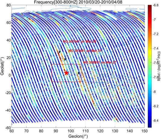
FIGURE 1. The variation of extremely low frequency magnetic field wave intensity during the 2010 April 6, Mw 7.8 Sumatra earthquake from March 20 to April 8, 2010, represented by power spectral density (PSD) values at frequency range (300–800 Hz). The red star denotes the epicenter, the red rectangle indicates the area of study. The horizontal and vertical axis represent the geo-longitude and latitude, respectively; the PSD values are color coded along the orbit trajectories.

FIGURE 2

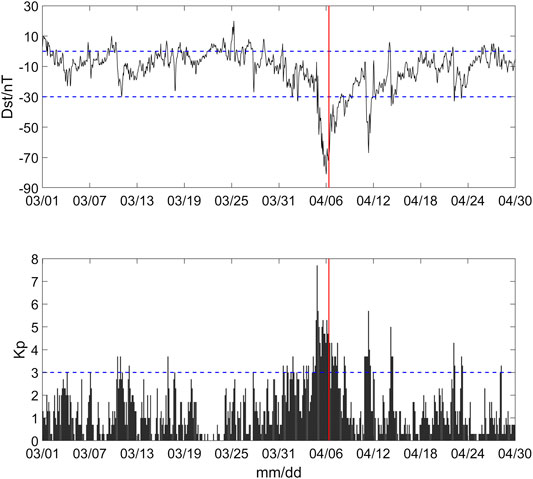
FIGURE 2. The geomagnetic field disturbance index from March to April 2010 (top: Dst, bottom: Kp). The vertical red lines represent the occurrence of the main shock. The horizontal dashed blue lines represent the thresholds for data selection applied in the study (for more details, see the main text).

It is not convincing to simply relate the enhancements of those orbits to the seismic activity just according to a short space and time window including the earthquake location and occurrence. We further selected previous observations along the same orbit trajectories (i.e., revisiting orbits) to investigate the long-term variation pattern. The sun-synchronous circular orbit feature of DEMETER allows the satellite to return to the same orbit trajectory at the same local time approximately every ∼13 days in 2010 (the recursive period changes due to the slight shift of satellite position). By using this feature of revisiting orbits, we can examine a longer time window to determine the normal electromagnetic environment background trend along the same orbital trace at the same local time.

According to Figure 1, we selected five orbits showing certain enhancements before the main shock which are: No. 306891 on March 27, No. 307041 on March 28, No. 307191 on March 29, No. 307921 on April 3, and No. 308071 on April 4, 2010, respectively. Then, we selected their corresponding revisiting orbits from August 2009 to May 2010 under quiet space weather conditions (Dst ≥ −30 nT and Kp ≤ 3). We also checked the solar activity during this half year period which kept a weak and stable level revealed by the sunspot numbers and there were no strong solar proton events occurring during this time period (not shown). We finally got 25 revisiting orbits for each of those above five orbits. The trajectories of those five orbits (colored) and their revisiting orbits (gray) are shown in Figure 3. Interestingly, in this time-window (August 2009 to May 2010), there was another earthquake occurred on March 5, 2010 with a magnitude of 6.8 in the vicinity of the 2010 Mw 7.8 northern Sumatra epicenter area (https://earthquake.usgs.gov/earthquakes/map), indicating that the fault movement in Sumatra area is very active. In Figure 3, the red star represents the April 6, 2010 Mw 7.8 EQ, and the orange one denotes the March 5, 2010 Mw 6.8 EQ.

FIGURE 3

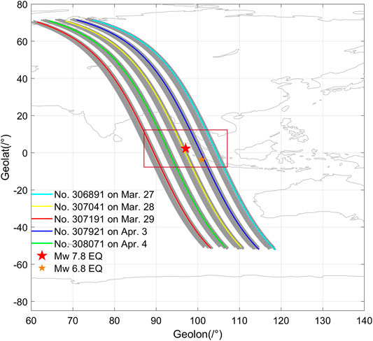
FIGURE 3. The trajectories of five orbits (No. 306891, 307041, 307191, 307921, and 308071, differently colored) with their revisiting orbits (gray lines) from August 2009 to May 2010. The red star represents the 2010 April 6, Mw 7.8 EQ, and the orange one denotes the 2010 March 5, Mw 6.8 EQ. The red rectangle represents the area of study.

According to the empirical equation of the earthquake preparation zone put forward by Dobrovolsky et al. (1979), the influential zone of a 7.8 magnitude earthquake in the lithosphere is a circle with a radius of 2,260 km. For convenience, considering the projection feature of satellite orbit on the ground, we chose a square area of around 1,800 km at satellite’s altitude, that is the epicenter (2.4°N, 97.1°E) ± 8° area, or (5.6°S–10.4°N, 89°E−105°E). We then extracted the PSD values at frequency (300–800 Hz) over the studied area from each revisiting orbit of the above five orbits, and re-sorted them as five sets of time-series data, and then we applied a running quartile method (Zhima et al., 2012b; Liu et al., 2013; Shen et al., 2017) to examine the long-term trend, as shown in Figure 4. The running medians, along with the inter-quartile ranges (IQR, being equal to the difference between the third and first quartiles) were computed by using the three previous and three successive orbits of the current orbit (7 orbits in total). We defined the running median PSD values as the background trend (denoted by blue lines in Figure 4), while the median PSD values of the current orbit as the current variation level (represented by red lines). The upper and lower bound were computed by the running median PSD values ± IQR values, denoted by the black and green lines, respectively. It can be seen in Figure 4 that three orbit trajectories, No. 306891, No. 307041, and No. 307921, show enhancements over the background trend before the two EQs. The recorded PSD values at frequency (300–800 Hz) along these three orbit trajectories are comparatively stable from August 2009 to February 2010, then start to fluctuate near the time of the two major shocks. However, the other two orbit traces at the west side of the epicenter (No. 307191, No. 308071, the last two panels in Figure 4) show no obvious difference between earthquake and non-earthquake time, it is difficult to identify any earthquake related abnormal signals from the variation pattern of the last two orbits, so we do not further discuss their relationship to earthquake any further.

FIGURE 4

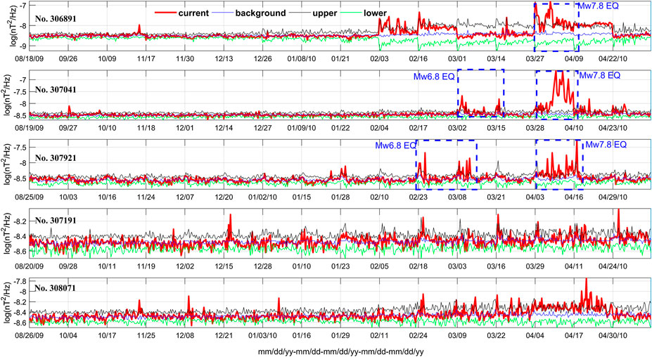
FIGURE 4. The long-term variation of wave intensities at extremely low frequency (300–800 Hz) revealed by the five orbits (No. 306891, 307041, 307191, 307921, and 308071) and their revisiting orbits recorded from August 2009 to May 2010. The red lines represent the current observation values, the blue ones denote the median values computed by data from 2009 to 2010, and the black and green lines are the upper/lower bounds (median values ± IQR values) also computed by data from 2009 to 2010.

Specifically, for the orbit No. 306891 (see the first panel in Figure 4), which recorded on the east side of epicenter on March 27, 2010, the PSD values reach to ∼10^–6.7 nT²/Hz before the Mw 7.8 EQ, far exceeding the background threshold (see the black and green lines). In addition, it shows a relatively smaller enhancement (∼10^–7.5 nT²/Hz) within one month before the Mw 6.8 EQ. The orbit No. 307041, which is located right above the Mw 7.8 epicenter (see Figure 3) on March 28, 2010, presents a low and stable trend until the time very near to the two major shocks, then it becomes strongly disturbed (see the second panel in Figure 4), reaching maximum values of ∼10^–7.8 nT²/Hz during the Mw 6.8 EQ, and ∼10^–6 nT²/Hz before the Mw 7.8 EQ. Along the orbit No. 307921, which closely passed over the Mw 6.8 epicenter area (see Figure 3) on April 3, 2010, the variation keeps a relative normal background trend far before the main shock time too, mainly gets disturbed on February 23, 2010 before the Mw 6.8 EQ, and after the Mw 6.8 EQ on March 8, and become highly enhanced from 10^–8.4 nT²/Hz to 10^–6.3 nT²/Hz during the Mw 7.8 EQ (see the third panel in Figure 4).

In all, the variation patterns of the above three orbits indicate that the wave intensity at frequency (300–800 Hz) indeed show enhancements with the location of during the Mw 7.8 EQ, compared to other quiet seismic activity times. Specifically, on March 27, 2010, 10 days before the Mw 7.8 EQ, the wave intensities started to increase with peak value around 10^–6.7 nT²/Hz on the orbit trace of No. 306891; and 3 days before the main shock, the wave intensities varied from 10^–8.4 to 10^–7.6 nT²/Hz along the orbit trace of No. 307921 (April 3). The strongest enhancement, of about 10^–6.0 nT²/Hz, was recorded along the orbit trace closest to the epicenter (No. 307041 on March 28) of the Mw 7.8 main shock.

Background Map

To obtain more convincing evidence of these abnormal ELF emissions, the longer term observations under quiet space weather condition (Dst ≥ −30nT and Kp ≤ 3) from 2008 to 2010 were selected to build a background map over the Mw 7.8 Sumatra EQ area. We extracted the data in a same-time-window from Feb. 1 to April 30 for each year from 2008 to 2010. Through this way, the variations related to the seasonal conditions can be eliminated.

In this study, we adopted the method put forward by Zhima et al. (2012a, 2012b) to build a background map based on longer-term satellite observations over the epicenter area. First, we extracted the observations over the area ±8° about the epicenter (5.6°S–10.4°N, 89°E–105°E) from February 1 to April 30 for each year, then computed the average PSD values of wave intensity. The average PSD values were binned as a function of latitude (5.6°S–10.4°N) and longitude (89°E–105°E) in steps of 2°. With these three-year data, we computed the median value of PSD values and the standard deviation value in each 2° × 2° bin and defined these data matrixes as β_2008–2010 and σ_2008–2010, respectively.

For 2010, the year of Mw 7.8 EQ, we built four data sets with four time intervals T_i (i = February 1 to February 28, March 1 to March 20, March 21 to April 6, April 7 to April 30, 2010, respectively). The median PSD values in each 2° × 2° bin for these four time-intervals were computed and defined as matrixes α_Ti,2010, respectively. Then we define the perturbation amplitude ∆ρ by Eq. 1 below:

$\Delta \rho =\left({\alpha }_{Ti\text{,}2010}-{\beta }_{2008–2010}\right)/{\sigma }_{2008–2010}(1)$

where ∆ρ is regarded as the perturbation amplitude during earthquake time T_i compared to the background map β_2008–2010. The difference between the magnetic field wave intensity at earthquake time (α_Ti,2010) and the long-term background map (β_2008–2010) is normalized by the standard deviation (σ_2008–2010) in each 2° × 2° data bin. We computed the ∆ρ for different frequency ranges from 300 to 800 Hz, and found that at the frequency range (468–566 Hz) there exists strong enhancements during the earthquake impending time [March 21–April 6, 2010] as shown in Figure 5.

FIGURE 5

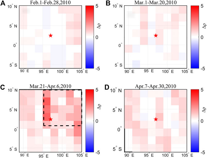
FIGURE 5. The ∆ρ distribution over the epicenter area computed by power spectral density values of magnetic field at frequency (468–566 Hz) during the 2010 Mw 7.8 Sumatra earthquake; (A) February 2 to February 28, 2010; (B) March 1 to March 20, 2010; (C) March 21 to April 6, 2010; (D) from April 7 to April 30, 2010. The star represents the 2010 Mw 7.8 Sumatra epicenter, the $\Delta \rho$ means the perturbation amplitude of current time intervals (a, b, c, d) relative to the background map built by observations from 2008 to 2010 (see text for explanation). The black dashed rectangle denotes the a wide scope area of power spectral density values’ enhancement.

Figure 5 shows the variation pattern of the perturbation amplitude ∆ρ during time intervals from February 1 to April 30, 2010. It can be seen that during the February 1 to March 20 time period (Figures 5A,B), the ∆ρ values in the epicenter area remain at a relatively low level, mostly varying around 0 and the maximum value peaking about 1.2. However, during the earthquake impending time interval from March 21 to April 6 (see Figure 5C), the $∆\rho$ gets enhanced (∼over 3), with the strongest enhancement mainly spread along the latitudinal direction of the near northwest side of the epicenter area (almost right above the epicenter). The eastern part of the epicenter gets a wide scope enhancement both along the longitudinal and latitudinal direction marked by the dashed square in Figure 5. After the main shock (Figure 5D), the $∆\rho$ returns back to a relatively low disturbance amplitude level, mostly around 0, and maximum value 1.2, similar to the levels in Figures 5A,B. Due to the disturbed space weather conditions, the observations during the earthquake impending days from April 3 to 6, 2010 (see Figure 2) were not included in this computation, so the enhancement showed in Figure 5C is very likely attributed to the seismic activity.

Wave Vector Analysis

We further checked the burst-mode observations which were automatically triggered when DEMETER flies above known seismic fault zones (Parrot et al., 2006a). The electromagnetic payloads ICE and IMSC in burst-mode provide six-components of waveform data at frequency range below 1.25 kHz with sampling rate of 2.5 kHz. However, the waveform data are not available at any time of interest during this earthquake. Fortunately, the orbit No. 306891 on March 27 (10 days before the main shock), and No. 307481 on March 31, 2010 (6 days before the main shock), coincidentally triggered burst-mode observations over the epicenter zone, allowing us to compute the wave propagation parameters by wave vector analysis method. Figure 6 shows the exact burst-mode operation locations of these two orbits.

FIGURE 6

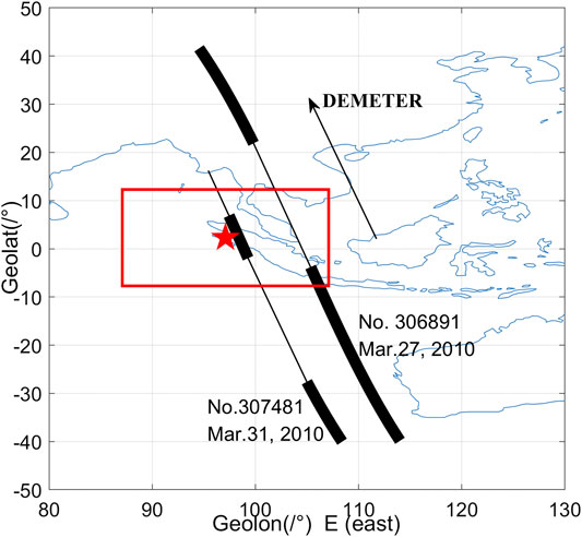
FIGURE 6. The available waveform data (thick lines) recorded by burst-mode observations near the seismic zone. The red rectangle is the area of study.

Figures 7A,B show the detailed electromagnetic spectral values computed by the waveform data of orbit No. 306891. It can be seen that near the epicenter area (2.38° N, 97.05°E), at the latitudes from ∼ 8° to 3.8°S, longitude from 107°E to ∼105°E, there exists electromagnetic wave activities (denoted by white arrows) mainly from 14:43 to 14:45 UT at L shells roughly from 1.4 to 1.09 where the satellite is quite near to the Mw 7.8 epicenter area.

FIGURE 7

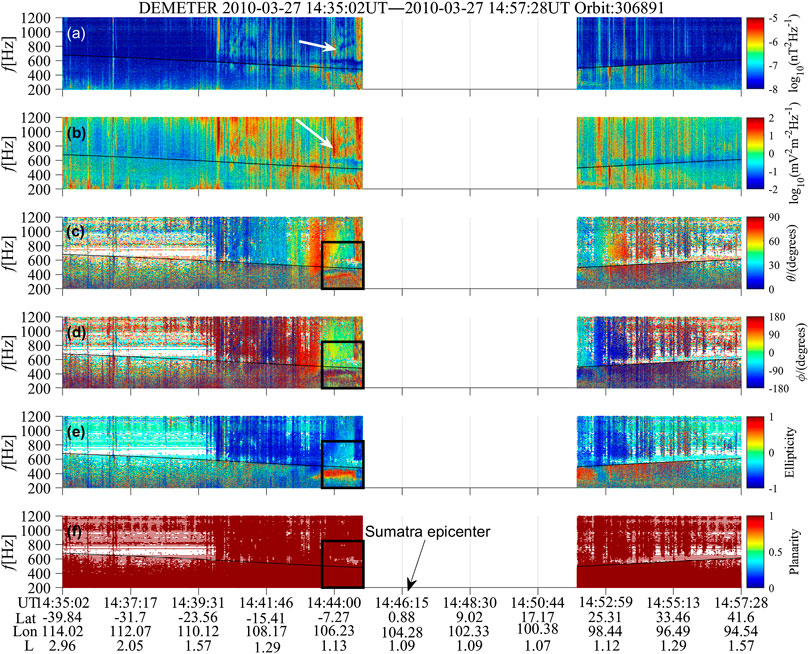
FIGURE 7. The wave propagation parameters of extremely low frequency waveform recorded by orbit No. 306891. The black lines represent the local proton cyclotron frequency. From top to bottom: (A,B) the power spectral values of magnetic field and electric field, (C) the wave normal angle θ; (D) the azimuthal angles ϕ; (E) the ellipticity, (F) the planarity. The arrow indicates the time of the orbit crosses the EQ epicenter. The black rectangular box denotes the abnormal waves near the epicenter area, which wave propagation parameters are statistically analyzed in Figure 8.

To compute the wave propagation parameters of these emissions over the epicenter zone, we built a Field Aligned Coordinate (FAC) system in the orbit space of DEMETER satellite. Under this FAC coordinate system, the Z-axis is along direction of the background magnetic field B₀, the Y-axis is horizontally perpendicular to the Z-axis cross the position vector of the satellite (so that the positive Y-axis is nominally eastward at the equator), and the X-axis completes the right-handed system. The background magnetic field B₀ is obtained by IGRF 2000 model (Olsen et al., 2000) according to DEMETER’s position. The angles θ and ϕ are defined as the wave normal angle (polar angle) and the azimuthal angle between the B₀ and the wave vector k. A value of 180° in azimuthal angle ϕ indicates that k propagates toward decreasing L shell direction, i.e., downward to the Earth direction, while 0° means that k propagates toward the increasing L shell direction in the meridian plane (i.e., from the Earth direction upward to the outer space direction). Then, the Singular Value Decomposition method put forward by Santolik et al. (2003) to compute wave propagation parameters, which has been widely used in the analysis of ELF/VLF space electromagnetic waves (Parrot et al., 2006b; Wei et al., 2007; Zhima et al., 2015a; Zhima et al., 2015b), was adopted to compute the wave normal angles, ellipticity, polarization, and planarity.

The computed wave propagation parameters from No. 306891 are shown in Figures 7C–F. The parameters computed by the low intensity waveform data (lower than 10^–7.8 nT²/Hz) are not shown for a better visual inspection. The wave normal angles θ of wave vector k are displayed in Figure 7C, which varies roughly from 40° to 80°, indicating these emissions are obliquely propagating. Figure 7D shows the azimuthal angles ϕ with a wide varying range from 0° to 180°. However, it can be clearly identified that there are some portions of emissions showing azimuthal angles ϕ ∼ 0° (see the black squares) mainly at frequency from 300 to 800 Hz (even up to ∼1,100 Hz) at ∼14:43:44 to 14:44:58 UT. According to the FAC coordinate system defined above, the propagation direction of these portions of emissions points upward from the Earth direction to the outer space direction (increasing L shell), indicating that these waves come from lower altitudes than the satellite.

It is noted that the strong emissions around 400–450 Hz with wave normal angles θ ∼ 90° (Figure 7C), azimuthal angles ϕ ∼ 180° (Figure 7D), the right handed ellipticity values of 1, are obliquely propagating downward from the higher altitudes (or decreasing L shell direction) than satellite position to the Earth direction, and they are identified as ionospheric hiss waves which might originate from the plasmasphere or the inner magnetosphere (Chen et al., 2017; Zhima et al., 2017; Xia et al., 2019), these emissions are not related to the earthquake activity.

The ellipticity values are given in Figure 7E, which represent the ratio of the axes of the polarization ellipse. The value +1 of ellipticity means that the wave is right-hand polarized, while −1 indicates that the wave is left-hand polarized, while 0 is the linearly polarized. For these portions of upward propagation waves (azimuthal angles ϕ ∼ 0°) the ellipticity mainly varies around 0 at frequencies 300–400 Hz, meaning that they are linearly polarized, while at frequencies below 300 Hz or above 450–800 Hz, even up to 1,100 Hz, the waves change to the left hand polarized (ellipticity varying from 0 to −1). The planarity of waves, which represents wave propagating in a single plane (+1) or in spherical direction (0), is presented in Figure 7F, with a value mostly being +1, implying that the observed waves are coming toward the spacecraft as plane wave propagation.

We also statistically analyzed the distributions of wave propagation parameters for the waves at frequency range (300–800 Hz) marked by the black square area in Figure 7 (including the downward right-handed hiss at frequency 400–450 Hz), as shown in Figure 8. The overlapped red curves represent the fitted curves computed by the kernel density distribution function. The majority of wave normal angles θ varies below 80°. The azimuthal angles ϕ mainly peaked at 0°. The ϕ values of ±180° are mostly attributed to the downward hiss waves at 400–450 Hz. For the ellipticity, the values of -0.5 to −1 are mostly related to the upward direction waves, and +1 to the downward hiss waves. The planarity predominates at values of 1.

FIGURE 8

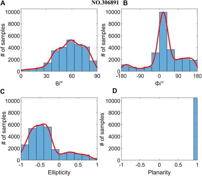
FIGURE 8. Distribution of wave propagation parameters for the waves in extremely low frequency (300–800 Hz) in the area (7.4°–3.8°S, 106.1°–105.6°E) recorded by No. 306891 at ∼14:44 to 14:45 UT, marked by the black square in Figure 7. The overlapped red lines represent fitted curves computed by a probability density function; (A) wave normal angle θ; (B) and azimuth angle ϕ of the wave vector; (C)the ellipticity; (D) planarity.

As with orbit No. 306891, the wave propagation parameters of waveform data for orbit No. 307481 at 15:08–15:10 UT on March 31, 2010 are shown in Figure 9. As can be seen from Figure 9 that the waveforms recorded at latitudes from 1.95°S to 6.8°N, longitudes from 99.29°E to 97.44°E are exactly over the epicenter zone (see Figure 5). The strong electromagnetic emissions along this orbit mainly appeared at frequencies below 500 Hz. The wave propagation parameters also show basically similar features as the waves recorded by No. 306891, although they are not as significant as the ones of No. 306891. However, it can be clearly identified that there are waves with azimuthal angles ϕ of 0°. Figure 10 shows the statistical features of the waves recorded from (1.95°S–6.89°N, 99.29°–97.44°E). For these waves, the wave normal angles θ vary at a broad range from 0° to 90°, indicating waves are obliquely propagating. The azimuthal angles ϕ have three peaks: ±180° and 0°, meaning there are waves mixed both from the Earth direction (ϕ = 0) and the outer space direction (ϕ = ±180°). The ellipticity mainly peaks around ±0.5, and the planarity is 1.

FIGURE 9

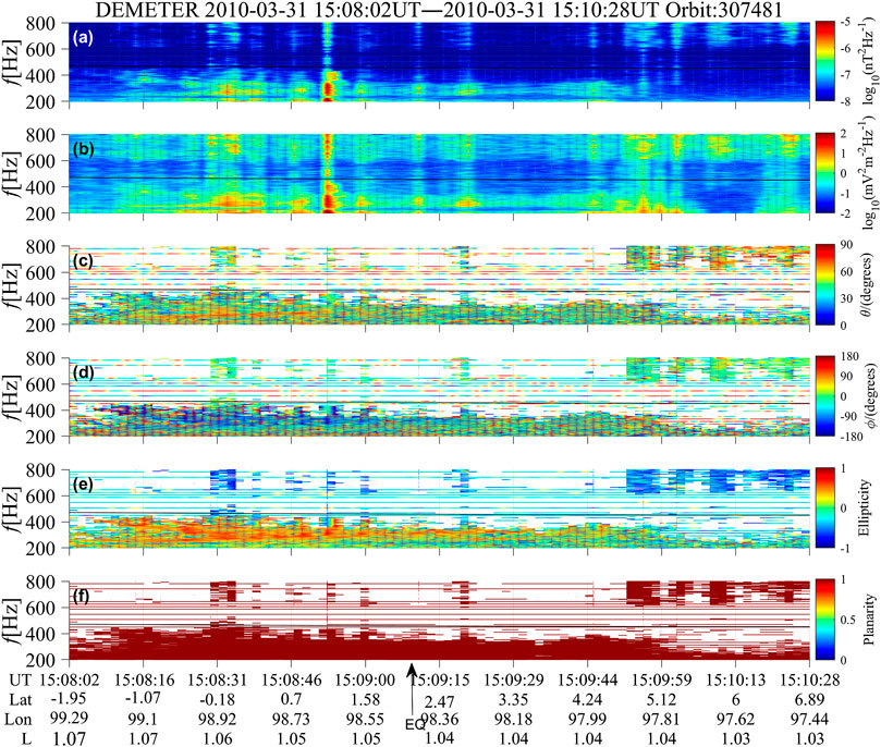
FIGURE 9. The wave propagation parameters of extremely low frequency waves recorded by orbit No. 307481 at 15:08 to 15:10 UT on March 31, 2010. From top to bottom: (A,B) the power spectral values of magnetic field and electric field, (C) the wave normal angle θ; (D) the azimuthal angles ϕ; (E) the ellipticity, (F) planarity.

FIGURE 10

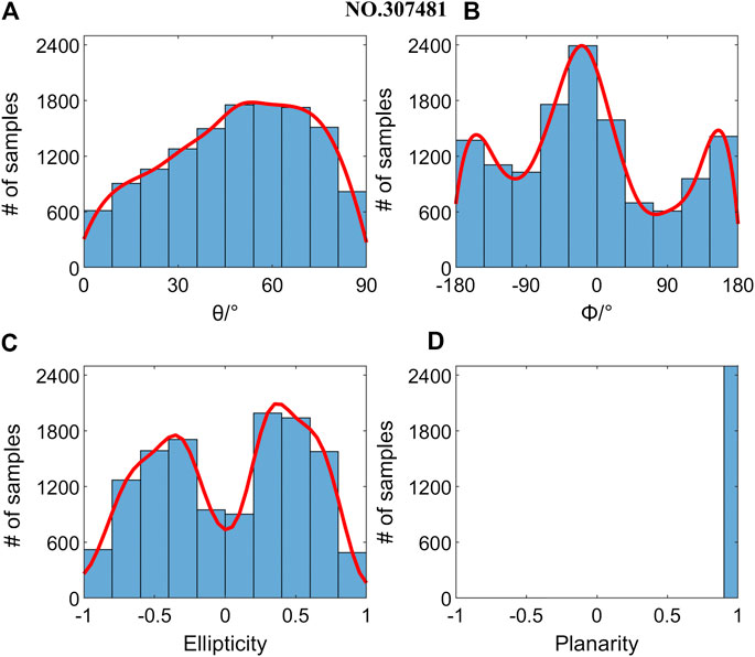
FIGURE 10. Distribution of wave propagation parameters for the waves at extremely low frequency (300–800 Hz) in the area (1.95°S–6.89°N, 99.29°−97.44°E) at 15:08 to 15:10 UT recorded by No. 307481 on March 31, 2010. The overlapped red lines represent fitted curves computed by a probability density function; (A) wave normal angle θ; (B) and azimuth angle ϕ of the wave vector; (C) the ellipticity; (D) planarity.

Discussions

The 2010 Mw 7.8 northern Sumatra EQ occurring at the equatorial area over where the equatorial ionosphere has less energetic particle precipitations compared to the high-latitude ionosphere, we do not need to consider the possibility of energetic particle precipitation induced wave activity in this study. Considering that the upper ionosphere environment space weather conditions are quiet during the studied time-window, there are two major generation sources for electromagnetic emissions we must consider: the atmosphere lightning activities and ground-based VLF transmitters.

The lightning activities from the atmosphere also serve as an embryonic source for strong ELF/VLF emissions in the upper ionosphere (Santolík et al., 2009; Shklyar et al., 2012; Zhima et al., 2017). The azimuthal angles of wave vector of lightning induced ELF/VLF emissions usually predominate around 0° (Zhima et al., 2017) in the above defined FAC coordinate system, which means that this kind of wave propagation direction points away from the Earth direction to outer space (in the increasing L shell direction). The lightning induced wave also presents either right or left handed polarization (Santolík et al., 2009), but most importantly, the lightning induced ELF/VLF emissions usually appear as a series of intensive burst spectra with vertical lines or whistler-mode falling/rising tones along the whole frequency range from a few hertz up to over 3 kHz or even 10 kHz (Zhima et al., 2017). In this study, the strong ELF emissions over the Sumatra epicenter zone appeared in a much lower frequency range (below 1,100 Hz), mainly at 300–800 Hz. Additionally, the variations of revisiting orbits also confirm that these emissions mainly get enhanced near earthquake time, while keeping a relatively smooth trend during the quiet-seismic activity time. Further, the perturbation amplitude relative to the background map also indicates that the enhancement of wave intensity at 300–800 Hz mainly occurs during the earthquake impending time intervals (see Figure 5C) but not in other time windows. So we exclude the possibility of lightning activity as the generation source for these abnormal ELF emissions.

Another kind of known electromagnetic emissions which can propagate from lithosphere to ionosphere are the artificial VLF radio waves emitted by the powerful ground-based VLF transmitters. VLF radio waves are mainly used as long-distance communication and navigation in the lithosphere-ionosphere waveguide, however, some portions of VLF radio wave energies leak into the ionosphere, propagating upward and reaching to satellite altitudes. The satellite recorded VLF radio waves usually appear at frequencies over 10 kHz to even to 30 kHz (Zhao et al., 2019), the spectra of VLF radio waves recorded by satellite usually exhibit a narrow transversal spectrum peak at the central frequency of the emitted radio waves (Shen et al., 2017; Zhang et al., 2018). Additionally, no VLF transmitter is reported near Sumatra area. So the association with VLF radio waves is excluded as a possible explanation of the observations presented here.

Previous studies (Sorokin et al., 2001; Sorokin et al., 2003; Molchanov et al., 2004; Pulinets and Ouzounov, 2011; Pulinets et al., 2018) have been undertaken to interpret the mechanism of the electromagnetic disturbances induced by earthquakes. Pulinets and Ouzounov (2011) presented the LAIC mechanism based on a complex multidisciplinary approach, trying to interpret the physical processes involved in generation of anomalous atmospheric and ionospheric phenomena associated with strong earthquakes.

First, the lithospheric rock due to tectonics plate movement, are stressed and release radon or other different kinds of gases into air (e.g., methane, helium, hydrogen, and carbon dioxide); subsequently, the radon radiation in the atmosphere changes the air conductivity resulting in a vertical electric current (see Figure 10 in Pulinets and Ouzounov (2011) and Figure 6 in Sorokin et al. (2001)). Correspondingly, the local growth of electric currents in the atmosphere develops AGW instabilities as well as a horizontal inhomogeneity of ionospheric conductivity (Sorokin et al., 2001), finally generating the magnetic field aligned currents, plasma irregularity or the ULF/ELF emissions (Sorokin et al., 2001). For example, during the 2004 Mw 9.0 Sumatra-Andaman EQ, a clear co-seismic AGW instability appeared in the atmosphere at VLF from 1.4 to 2.8 mHz with a group velocity around 300–314 m/s and amplitudes varying from ∼1 to 12 Pa (Mikumo et al., 2008).

AGW can be evaluated by the wind field and temperature data and the total wave energy (E₀) of AGW can be described by the sum of kinetic (E_K) and potential energies (E_P) which correspond to the fluctuations in the wind field and temperature of atmosphere (Yang et al., 2019), respectively. E₀ and E_P energies are proportional to each other (VanZandt, 1985; de la Torre et al., 1999), so that we can examine AGW instability through E_P, which is defined as (VanZandt, 1985; Yang et al., 2019):

$E_P=\frac{1}{2}{\left(\frac{g}{N}\right)}^2\overline{{\left(\frac{T^{\text{'}}}{\overline{T}}\right)}^2}(2)$

where g is the gravitational acceleration constant (9.8 ms⁻²), $T^{\text{'}}$ is the perturbation atmosphere temperature deviated from the background temperature $\overline{T}$. N is the Brünt-Vaisala frequency defined as (Fritts and Alexander, 2003):

$N=\sqrt{\frac{g}{\theta }\frac{d\theta }{dz}}(3)$

where N is a function of altitude and potential temperature, where $\theta =T{\left(\frac{P_0}{P}\right)}^{\frac{R}{c_p}}$ is the potential temperature, z is the altitude, P₀ is the standard reference pressure (1 hPa), P is air pressure, R is the gas constant of air and c_p is the specific heat capacity at a constant pressure, R/c_p = 0.286 for air.

The variance term $\overline{{\left(\frac{T^{\text{'}}}{\overline{T}}\right)}^2}$ is calculated within a layer of 2 km thickness as:

$\overline{{\left(\frac{T^{\text{'}}}{\overline{T}}\right)}^2}=\frac{1}{z^{max}-z^{min}}\underset{z^{min}}{\overset{z^{max}}{{\displaystyle \int }}}{\left(\frac{T^{\text{'}}}{\overline{T}}\right)}^{2}dz(4)$

where z_max and z_min are the top and bottom altitudes of the layer.

Here we computed the E_P variation over the 2010 Sumatra epicenter area by using the technique developed by Yang et al. (2019) with some procedures modified to fit in the ERA-5 data, as shown in Figure 11. Figure 11A shows the vertical temperature profile retrieved from ERA-5 dataset over the Sumatra EQ epicenter, and Figure 11B is the background temperature from Figure 11A filtered by a moving average of every 2 km; Figure 11C displays the temperature deviation computed by removing the background from the original temperature profile; Figure 11D represents the squared term of the Brunt-Väisälä frequency computed by Eq. 3 with the temperature profile; Figure 11E is the potential energy as calculated by Eq. 2.

FIGURE 11

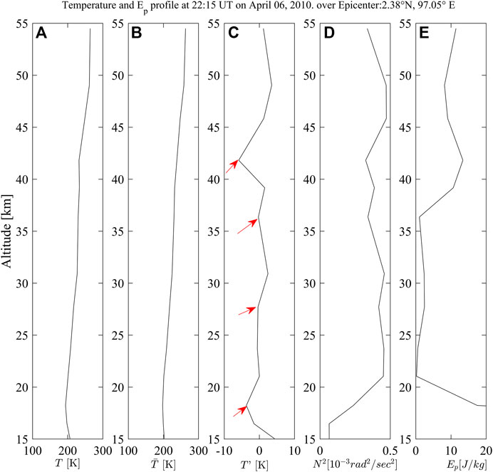
FIGURE 11. The simulation of Acoustic Gravity Waves propagation over the 2010 Mw 7.8 Sumatra epicenter. From left to right: (A) the vertical temperature profile retrieved from ERA-5 dataset; (B) the background temperature profile filtered by an every 2 km moving average of Figure 11A; (C) the temperature deviation between Figures 11A,B; (D) the squared term N² of the Brunt-Väisälä frequency; (E) the potential energies (E_P) computed over epicenter area.

It can be seen from Figure 11E that the E_P value peaks around the altitude of 17 km (the tropopause), which is a common phenomenon (Yang et al., 2019). Four wave crests can be identified in the temperature deviation profile at the altitudes of 18.23, 27.71, 36.36, and 41.82 km (denoted by arrows in Figure 11C). We computed the wavelength of a full sinusoidal period of these four wave crests in the temperature deviation but not in the E_P profile. The corresponding vertical wavelengths are 9.5, 8.7, and 5.5 km for the four wave crests, which are consistent with previous understanding that the vertical wavelength of stratospheric AGW is about 2–10 km (Tsuda et al., 1994). Therefore, we suggest the possible existence of AGW wave in the atmosphere at the moment of the 2010 Sumatra EQ occurrence.

It must be admitted that through this computation, we only found the possibility of AGW generation during main shock. Because of the complicated LAIC coupling mechanism, it is impossible to build a coupling model at every key altitude (or layer) from the lithosphere to the satellite’s location, and to evaluate how the coupling processing is developing. Anyway, we can tentatively interpret the link between the AGW propagation and the electric field observations in terms of a mechanical interaction between the atmospheric pressure gradient induced by the AGW and the ionosphere which causes a local instability in the plasma distribution. Such plasma variation gives rise, in the E-layer, to a local non-stationary electric current which, successively, generates an electromagnetic (EM) wave (Yang 2019; Piersanti et al., 2020, submitted).

The interpretation of LAIC mechanism needs a multidisciplinary synergy (Pulinets and Ouzounov, 2011) with the simultaneous observational data at different altitudes in lithosphere-atmosphere-ionosphere system which are sensitive to various kinds of disturbances. The relatively very weak precursors of earthquakes can be submerged by other stronger perturbations even during quiet space weather conditions. At present, the LAIC mechanism still lacks reliable experimental evidence with direct and simultaneous observations at different layers or altitudes. It involves geophysical, chemical and even biological knowledge to interpret the mystery of seismic-ionospheric coupling. Many of the reported seismic-ionospheric case studies still require the further experimental confirmation and objective statistical studies.

Conclusions

This paper investigated the abnormal electromagnetic emissions during the 2010 April 6 Mw 7.8 Sumatra earthquake based on DEMETER satellite observations. The PSD values show that there are certain enhancements of wave intensity at frequency range (300–800 Hz) on 10–3 days before the main shock. The variation patterns along the same orbit trajectories which were computed from the revisiting orbits (August 2009 to May 2010) further indicate that the wave intensity indeed got enhanced during seismic activity time compared to the relatively stable variation patterns during quiet seismic activity time. Specifically, on March 28, 2010 (9 days before main shock), the wave intensity started to increase with peak value around 10^–6.7 nT²/Hz on the orbit trace of No. 306891 (3 days before the main shock), the wave intensity varied from 10^–8.4 to 10^–6.3 nT²/Hz along the orbit trace of No. 307921. The strongest enhancement of 10^–6.0 nT²/Hz was recorded along the orbit trace nearest to the epicenter (No. 307041).

We further investigated the perturbation amplitude relative to the background map which is built by four years’ of quiet space weather time data using the same time window (each year from February 1 to April 30), and found that the perturbation amplitude of wave intensities at frequency range (468–566 Hz) were indeed enhanced during the earthquake impending time interval (from March 21 to April 6).

We further computed the wave propagation parameters for the electromagnetic field waveform data by using Singular Value Decomposition method. Results show that there does exist some portions of ELF emissions mainly at 300–800 Hz, propagating upward from some altitudes lower than the satellite over the seismic zone. We excluded other generation sources for ELF/VLF emissions under quiet space weather conditions, such as the lightning activity and ground-based VLF transmitters. Considering the wave propagation features and their locations, we suggest that these portions of upward propagating ELF waves are very likely excited during the earthquake preparation processing.

According to the previous studies (e.g., Gokhberg et al., 1982; Larkina et al., 1989; Bhattacharya et al., 2007; Błeçki et al., 2010; Zhima et al., 2012a; Zhima et al., 2012b; Pulinets et al., 2018) and the reference therein, it is sure that the ELF electromagnetic emission is a promising tool for earthquake precursor detection. It usually appears a few days or weeks over the earthquake preparation zone, especially during the impend moment of a shock rupture in which the variation of stress on the rocks excite electromagnetic emissions at a broad band.

In this study we mainly took an approach of extraction the anomaly information before the strong earthquake by a case study. We didn’t involve the aftershock effects in this study. We will leave it for future deep research after we accumulated enough evidence for the abnormal seismic emissions from satellite observations.

For the possible mechanism, we computed the potential energy of AGW at the moment of earthquakes and results confirm the possible existence of AGW with wavelength roughly varying from 5.5 to 9.5 km in the atmosphere at the moment of the main shock. It must be admitted that in this study, we just suggest the possibility of AGW generation over the epicenter area, due to the very complicated LAIC coupling mechanism and the impossibility of building a coupling model at every key altitude (or layer) from lithosphere to ionosphere space with the present day’s science and technology levels. The comprehensive interpretation on the LAIC is beyond the scope of the present study, but we hope to explore this topic in the future.

Data Availability Statement

The datasets presented in this study can be found in online repositories. The names of the repository/repositories and accession number(s) can be found below: DEMETER: http://demeter.cnrs-orleans.fr/. The geomagnetic index: https://cdaweb.sci.gsfc.nasa.gov/index.html/. ECMWF ERA5: https://www.ecmwf.int/en/forecasts/datasets/reanalysis-datasets/era5.

Author Contributions

ZZ: scientific analysis and manuscript writing. YH: data collection and data processing. MP: AGW wave simulation and its scientific analysis. XS and AS: scientific analysis. RY, YY, SZ, ZZ, QW, JH, and FG: data collection and scientific analysis

Conflict of Interest:

The authors declare that the research was conducted in the absence of any commercial or financial relationships that could be construed as a potential conflict of interest.

The reviewer (MP) declared a past co-authorship with some of the authors (ZZ, RY) to the handling editor.

Funding

This work was supported by NSFC Grant 41874174, 41574139, National Key R&D Program of China (Grant No. 2018YFC1503501), the NSFC Grant 41904149, the APSCO Earthquake Research Project Phase II and ISSI-BJ project. MP and ADS thank Italian Space Agency (ASI) for the financial support under the contract ASI “LIMADOU scienza” no. 2016-16-H0. ADS received partial funds by SAFE Project funded by ESA (European Space Agency).

Acknowledgments

We acknowledge DEMETER scientific mission center for providing observations of electromagnetic field (http://demeter.cnrs-orleans.fr/). The geomagnetic index Kp and Dst index is provided by (https://cdaweb.sci.gsfc.nasa.gov/index.html/); the vertical temperature profile data of atmosphere are available through the ECMWF Web Applications Server (https://www.ecmwf.int/en/forecasts/datasets/reanalysis-datasets/era5). The authors sincerely thank Marc Hairston of the University of Texas at Dallas for assistance in copyediting this paper.

References

Bertello, I., Piersanti, M., Candidi, M., Diego, P., and Ubertini, P. (2018). Electromagnetic field observations by the DEMETER satellite in connection with the 2009 L’Aquila earthquake. Ann. Geophys. 36, 1483–1493. doi: 10.5194/angeo-36-1483-2018

CrossRef Full Text | Google Scholar

Berthelier, J. J., Godefroy, M., Leblanc, F., Malingre, M., Menvielle, M., Lagoutte, D., et al. (2006). ICE, the electric field experiment on DEMETER. Planet. Space Sci. 54 (5), 456–471. doi: 10.1016/j.pss.2005.10.016

CrossRef Full Text | Google Scholar

Bhattacharya, S., Sarkar, S., Gwal, A., and Parrot, M. (2007). Satellite and ground-based ULF/ELF emissions observed before Gujarat earthquake in March 2006. Curr. Sci. 93 (1), 41–46. http://www.jstor.org/stable/24099425

Google Scholar

Błeçki, J., Parrot, M., and Wronowski, R. (2010). Studies of the electromagnetic field variations in ELF frequency range registered by DEMETER over the Sichuan region prior to the 12 May 2008 earthquake. Int. J. Remote Sens. 31 (13), 3615–3629. doi: 10.1080/01431161003727754

CrossRef Full Text | Google Scholar

Chen, L., Santolík, O., Hajoš, M., Zheng, L., Zhima, Z., Heelis, R., et al. (2017). Source of the low‐altitude hiss in the ionosphere. Geophys. Res. Lett. 44, 2060. doi: 10.1002/2016GL072181

CrossRef Full Text | Google Scholar

de la Torre, A., Alexander, A. P., and Giraldez, A. (1999). The kinetic to potential energy ratio and spectral separability from high-resolution balloon soundings near the Andes Mountains. Geophys. Res. Lett. 26 (10), 1413–1416. doi: 10.1029/1999gl900265

CrossRef Full Text | Google Scholar

Dobrovolsky, I. P., Zubkov, S. I., and Miachkin, V. I. (1979). Estimation of the size of earthquake preparation zones. Pure. Appl. Geophys. 117, 1025–1044. doi: 10.1007/bf00876083

CrossRef Full Text | Google Scholar

Fritts, D. C., and Alexander, M. J. (2003). Gravity wave dynamics and effects in the middle atmosphere. Rev. Geophys. 41, 1–68. doi: 10.1029/2001rg000106

CrossRef Full Text | Google Scholar

Gokhberg, M. B., Morgounov, V. A., Yoshino, T., and Tomizawa, I. (1982). Experimental measurement of electromagnetic emissions possibly related to earthquakes in Japan. J. Geophys. Res. 87 (B9), 7824. doi: 10.1029/JB087iB09p07824

CrossRef Full Text | Google Scholar

Heki, K., Otsuka, Y., Choosakul, N., Hemmakorn, N., Komolmis, T., and Maruyama, T. (2006). Detection of ruptures of Andaman fault segments in the 2004 great Sumatra earthquake with coseismic-ionospheric disturbances. J. Geophys. Res. 111 (B9), B09313–B09311. doi: 10.1029/2005jb004202

CrossRef Full Text | Google Scholar

Henderson, T. R., Sonwalkar, V. S., Helliwell, R. A., Inan, U. S., and Fraser-Smith, A. C. (1993). A search for ELF/VLF emissions induced by earthquakes as observed in the ionosphere by the DE 2 satellite. J. Geophys. Res. 98, 9503–9514. doi: 10.1029/92ja01533

CrossRef Full Text | Google Scholar

Huang, Q., and Ikeya, M. (1998). Seismic electromagnetic signals (SEMS) explained by a simulation experiment using electromagnetic waves. Phys. Earth Planet. Inter. 109 (3), 107–114. doi: 10.1016/s0031-9201(98)00135-6

CrossRef Full Text | Google Scholar

Kumar, A., Kumar, S., Hayakawa, M., and Menk, F. (2013). Subionospheric VLF perturbations observed at low latitude associated with earthquake from Indonesia region. J. Atmos. Sol. Terr. Phys. 102, 71–80. doi: 10.1016/j.jastp.2013.04.011

CrossRef Full Text | Google Scholar

Lagoutte, D., Brochot, J. Y., De Carvalho, D., Elie, F., Harivelo, F., Hobara, Y., et al. (2006). The DEMETER science mission centre. Planet. Space Sci. 54 (5), 428–440. doi: 10.1016/j.pss.2005.10.014

CrossRef Full Text | Google Scholar

Larkina, V. I., Migulin, V. V., Molchanov, O. A., Kharkov, I. P., Inchin, A. S., and Schvetcova, V. B. (1989). Some statistical results on very low frequency radiowave emissions in the upper ionosphere over earthquake zones. Phys. Earth Planet. Inter. 57 (1), 100–109. doi: 10.1016/0031-9201(89)90219-7

CrossRef Full Text | Google Scholar

Liu, J., Zhang, X., Novikov, V., and Shen, X. (2016). Variations of ionospheric plasma at different altitudes before the 2005 Sumatra Indonesia M s 7.2 earthquake. J. Geophys. Res. Space Phys. 121 (9), 9179–9187. doi: 10.1002/2016ja022758

CrossRef Full Text | Google Scholar

Liu, J. Y., Chen, Y. I., Chen, C. H., and Hattori, K. (2010). Temporal and spatial precursors in the ionospheric global positioning system (GPS) total electron content observed before the 26 December 2004 M9.3 Sumatra–Andaman Earthquake. J. Geophy. Res. 115 (A9), A09312–A09313. doi: 10.1029/2010ja015313

CrossRef Full Text | Google Scholar

Liu, J. Y., Wang, K., Chen, C. H., Yang, W. H., Yen, Y. H., Chen, Y. I., et al. (2013). A statistical study on ELF-whistlers/emissions and M ≥ 5.0 earthquakes in Taiwan. J. Geophys. Res. Space Phys. 118 (6), 3760–3768. doi: 10.1002/jgra.50356

CrossRef Full Text | Google Scholar

Marchetti, D., De Santis, A., Shen, X., Campuzano, S. A., Perrone, L., Piscini, A., et al. (2020). Possible lithosphere-atmosphere-ionosphere coupling effects prior to the 2018 Mw = 7.5 Indonesia earthquake from seismic, atmospheric and ionospheric data. J. Asian Earth Sci. 188, 104097. doi: 10.1016/j.jseaes.2019.104097

CrossRef Full Text | Google Scholar

Mikumo, T., Shibutani, T., Le Pichon, A., Garces, M., Fee, D., Tsuyuki, T., et al. (2008). Low-frequency acoustic-gravity waves from coseismic vertical deformation associated with the 2004 Sumatra-Andaman earthquake (Mw = 9.2). J. Geophys. Res. 113 (B12), B12402–B12411. doi: 10.1029/2008jb005710

CrossRef Full Text | Google Scholar

Molchanov, O., Fedorov, E., Schekotov, A., Gordeev, E., Chebrov, V., Surkov, V., et al. (2004). Lithosphere-atmosphere-ionosphere coupling as governing mechanism for preseismic short-term events in atmosphere and ionosphere. Nat. Hazards Earth Syst. Sci. 4, 757–767. doi: 10.5194/nhess-4-757-2004

CrossRef Full Text | Google Scholar

Molchanov, O., Rozhnoi, A., Solovieva, M., Akentieva, O., Berthelier, J. J., Parrot, M., et al. (2006). Global diagnostics of the ionospheric perturbations related to the seismic activity using the VLF radio signals collected on the DEMETER satellite. Nat. Hazards Earth Syst. Sci. 6, 745–753. doi: 10.5194/nhess-6-745-2006

CrossRef Full Text | Google Scholar

Nemec, F., Santolik, O., and Parrot, M. (2009). Decrease of intensity of ELF/VLF waves observed in the upper ionosphere close to earthquakes: a statistical study. J. Geophys. Res. 114 (A04303), 1–10. doi: 10.1029/2008JA013972

CrossRef Full Text | Google Scholar

Olsen, N., Sabaka, T. J., and Tøffner-Clausen, L. (2000). Determination of the IGRF 2000 model. Earth Planets Space. 52, 1175–1182. doi: 10.1186/bf03352349

CrossRef Full Text | Google Scholar

Parrot, M. (1989). VLF emissions associated with earthquakes and observed in the ionosphere and the magnetosphere. Phys. Earth Planet. Inter. 57 (1–2), 86–99. doi: 10.1016/0031-9201(89)90218-5

CrossRef Full Text | Google Scholar

Parrot, M. (1994). Statistical study of ELF/VLF emissions recorded by a low-altitude satellite during seismic events. J. Geophys. Res. 99 (A12), 23339. doi: 10.1029/94ja02072

CrossRef Full Text | Google Scholar

Parrot, M., Benoist, D., Berthelier, J. J., Błęcki, J., Chapuis, Y., Colin, F., et al. (2006a). The magnetic field experiment IMSC and its data processing onboard DEMETER: scientific objectives, description and first results. Planet. Space Sci. 54 (5), 441–455. doi: 10.1016/j.pss.2005.10.015

CrossRef Full Text | Google Scholar

Parrot, M., Berthelier, J., Lebreton, J., Sauvaud, J., Santolik, O., and Blecki, J. (2006b). Examples of unusual ionospheric observations made by the DEMETER satellite over seismic regions. Phys Chem Earth Parts A/B/C 31 (4–9), 486–495. doi: 10.1016/j.pce.2006.02.011

CrossRef Full Text | Google Scholar

Pulinets, S., Ouzounov, D., and Davidenko, D. (2018). The possibility of earthquake forecasting: learning from nature. Bristol, UK: IOP Publishing. doi: 10.1088/978-0-7503-1248-6ch2

CrossRef Full Text | Google Scholar

Pulinets, S., and Ouzounov, D. (2011). Lithosphere-atmosphere-ionosphere coupling (LAIC) model - an unified concept for earthquake precursors validation. J. Asian Earth Sci. 41 (4), 371–382. doi: 10.1016/j.jseaes.2010.03.005

CrossRef Full Text | Google Scholar

Rodger, C. J., Thomson, N. R., and Dowden, R. L. (1996). A search for ELF/VLF activity associated with earthquakes using ISIS satellite data. J. Geophys. Res. 101 (A6), 13369–13378. doi: 10.1029/96ja00078

CrossRef Full Text | Google Scholar

Santolík, O., Parrot, M., Inan, U. S., Burešová, D., Gurnett, D. A., and Chum, J. (2009). Propagation of unducted whistlers from their source lightning: a case study. J. Geophys. Res. 114 (A3), A03212. doi: 10.1029/2008ja013776

CrossRef Full Text | Google Scholar

Santolik, M., Parrot, M., and Lefeuvre, F. (2003). Singular value decomposition methods for wave propagation analysis. Radio Sci. 38 (1), 1010. doi: 10.1029/2000RS002523

CrossRef Full Text | Google Scholar

Serebryakova, O. N., Bilichenko, S. V., Chmyrev, V. M., Parrot, M., Rauch, J. L., Lefeuvre, F., et al. (1992). Electromagnetic ELF radiation from earthquake regions as observed by low-altitude satellites. Geophys. Res. Lett. 19 (2), 91–94. doi: 10.1029/91gl02775

CrossRef Full Text | Google Scholar

Shen, X., Zhima, Z., Zhao, S., Qian, G., Ye, Q., and Ruzhin, Y. (2017). VLF radio wave anomalies associated with the 2010 Ms 7.1 Yushu earthquake. Adv. Space Res. 59 (10), 2636–2644. doi: 10.1016/j.asr.2017.02.040

CrossRef Full Text | Google Scholar

Shklyar, D. R., Storey, L. R. O., Chum, J., Jiříček, F., Němec, F., Parrot, M., et al. (2012). Spectral features of lightning-induced ion cyclotron waves at low latitudes: DEMETER observations and simulation. J. Geophys. Res. 117 (A12), 16. doi: 10.1029/2012ja018016

CrossRef Full Text | Google Scholar

Sorokin, V. M., Chmyrev, V. M., and Yaschenko, A. K. (2001). Electrodynamic model of the lower atmosphere and the ionosphere coupling. J. Atmos. Sol. Terr. Phys. 63 (16), 1681–1691. doi: 10.1016/s1364-6826(01)00047-5

CrossRef Full Text | Google Scholar

Sorokin, V. M., Chmyrev, V. M., and Yaschenko, A. K. (2003). Ionospheric generation mechanism of geomagnetic pulsations observed on the Earth’s surface before earthquake. J. Atmos. Sol. Terr. Phys. 65 (1), 21–29. doi: 10.1016/s1364-6826(02)00082-2

CrossRef Full Text | Google Scholar

Tsuda, T., Murayama, Y., Nakamura, T., Vincent, R. A., Manson, A. H., Meek, C. E., et al. (1994). Variations of the gravity wave characteristics with height, season and latitude revealed by comparative observations. J. Atmos. Terr. Phys. 56 (5), 555–568. doi: 10.1016/0021-9169(94)90097-3

CrossRef Full Text | Google Scholar

VanZandt, T. E. (1985). A model for gravity wave spectra observed by Doppler sounding systems. Radio Sci. 20 (6), 1323–1330. doi: 10.1029/RS020i006p01323

CrossRef Full Text | Google Scholar

Wei, X. H., Cao, J. B., Zhou, G. C., Santolík, O., Rème, H., Dandouras, I., et al. (2007). Cluster observations of waves in the whistler frequency range associated with magnetic reconnection in the Earth’s magnetotail. J. Geophys. Res. 112 (A10), A10225. doi: 10.1029/2006ja011771

CrossRef Full Text | Google Scholar

Xia, Z., Chen, L., Zhima, Z., Santolík, O., Horne, R. B., and Parrot, M. (2019). Statistical characteristics of ionospheric hiss waves. Geophys. Res. Lett. 46 (13), 7147–7156. doi: 10.1029/2019GL083275

CrossRef Full Text | Google Scholar

Yang, S. S., Asano, T., and Hayakawa, M. (2019). Abnormal gravity wave activity in the stratosphere prior to the 2016 Kumamoto earthquakes. J. Geophys. Res. Space Phys. 124 (2), 1410–1425. doi: 10.1029/2018ja026002

CrossRef Full Text | Google Scholar

Zhang, Z., Chen, L., Li, X., Xia, Z., Heelis, R. A., and Horne, R. B. (2018). Observed propagation route of VLF transmitter signals in the magnetosphere. J. Geophys. Res. Space Phys. 123 (7), 5528–5537. doi: 10.1029/2018ja025637

CrossRef Full Text | Google Scholar

Zhao, S., Zhou, C., Shen, X., and Zhima, Z. (2019). Investigation of VLF transmitter signals in the ionosphere by ZH‐1 observations and full‐wave simulation. J. Geophys. Res. Space Phys. 124 (6), 4697–4709. doi: 10.1029/2019ja026593

CrossRef Full Text | Google Scholar

Zhima, Z., Cao, J., Fu, H., Liu, W., Chen, L., Dunlop, M., et al. (2015a). Whistler mode wave generation at the edges of a magnetic dip. J. Geophys. Res. Space Phys. 120 (4), 2469–2476. doi: 10.1002/2014JA020786

CrossRef Full Text | Google Scholar

Zhima, Z., Chen, L., Fu, H., Cao, J., Horne, R. B., and Reeves, G. (2015b). Observations of discrete magnetosonic waves off the magnetic equator. Geophys. Res. Lett. 42 (22), 9694–9701. doi: 10.1002/2015GL066255

CrossRef Full Text | Google Scholar

Zhima, Z., Chen, L., Xiong, Y., Cao, J., and Fu, H. (2017). On the origin of ionospheric hiss: a conjugate observation. J. Geophys. Res. 122 (11), 11784–11793. doi: 10.1002/2017JA024803

CrossRef Full Text | Google Scholar

Zhima, Z., Xu-Hui, S., Jin-Bin, C., Zhang, X., Huang, J., Jing, L., et al. (2012a). Statistical analysis of ELF/VLF magnetic field disturbances before major earthquakes. Chinese J Geophys. 55, 3699–3708. doi: 10.6038/j.issn.0001-5733.2012.11.017

CrossRef Full Text | Google Scholar

Zhima, Z., Xuhui, S., Xuemin, Z., Jinbin, C., Jianping, H., Xinyan, O., et al. (2012b). Possible ionospheric electromagnetic perturbations induced by the Ms7. 1 Yushu earthquake. Earth Moon Planets. 108 (3–4), 231–241. doi: 10.1007/s11038-012-9393-z

CrossRef Full Text | Google Scholar