Groundwater characterization in arid regions using seismic and gravity attributes: Al Jaww Plain, UAE

Introduction

The United Arab Emirates (UAE), as other arid countries, rely heavily on nonconventional water resources, whose production requires expensive processes as desalination and waste water treatment. Groundwater overexploitation, mostly to meet the irrigation demand, affected groundwater productivity. It also caused seawater intrusion in the coastal areas and saline water upconing in the inland areas, where saline water horizons exist below fresh water horizons (El Mahmoudi, 2004). Quantitative and qualitative assessment of the groundwater resources is required for decision makers to outline future plans for groundwater development in that area. Such characterization is a key challenge not only for freshwater catchment but also for hydrocarbon production, geothermal energy generation, and fluid/gas sequestration. Geophysical methods can play a major role to quantify these resources and estimate their hydrogeological parameters. For example, seismic surveys can identify high impedance boundaries that can be linked to formation boundaries through borehole calibrations; they can also estimate formation thicknesses and provide clues about their porosity.

Aquifer assessment by seismic techniques has been validated in the past decades (see, e.g., Miller et al., 1986, Whiteley et al., 1998, Bradford and Sawyer, 2002, and Nieto et al., 2014, among many others), but reliability of the assessment increases when it is integrated by direct downhole measurements and by other independent geophysical methods. Cassiani et al. (1998) showed that a geostatistical link may be established between hydraulic conductivity and P-wave velocity, estimated by a tomographic inversion of traveltimes. However, this link may be feeble where the velocity contrast is small or when there is not a clear flat that may be interpreted as the water table. For these reasons, additional parameters are needed to reduce the interpretation uncertainties. Another property characterizing the near surface formations for their water saturation degree is the quality factor Q (Mavko et al., 1998; Prasad et al., 2005; Carcione, 2014). In this paper, we show that the coupled inversion of P velocity and Q factor and their statistical integration with seismic reflection images provide geophysical images that are consistent with the known surface and subsurface geology in the area, allowing to validate and better predict the aquifer characteristics in the subsurface.

We present an integrated processing flow that improves the knowledge of the tectonic framework and provides an integrated, geophysical characterization of shallow and deep water-bearing geological formations. We apply it to the Al Jaww Plain, a wide and prominent piedmont that provides a substantial share of UAE's fresh water resources. The Plain is located at the ESE of the city of Al Ain, between the Oman Mountains and Jabal Hafit (Figure 1). In this paper, we extend previous studies about this area (Al-Lazki et al., 2002;, Ali et al., 2008, and Ali et al., 2017) with the contribution of a new seismic profile, integrated by the reprocessing of published gravity data. We acquired a new 6-km-long seismic profile at the Eastern border of the plain, toward the Oman mountains (Figures 2, 3). We processed different seismic wave types, i.e., near-vertical and wide-angle reflected waves and direct and diving waves. We estimated from them different seismic parameters as reflectivity and other attributes (e.g., energy and similarity) as well as P-wave velocity and Q factor, obtaining a multivariate dataset for integration.

FIGURE 1

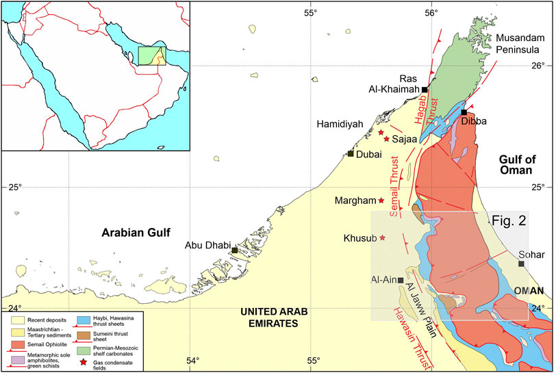
FIGURE 1. Simplified regional geological map of the UAE and Northern Oman Mountains, modified from Searle (2007) and Ali et al. (2008). The inset shows the location of the map (yellow rectangle) relative to the Arabian Peninsula. The shadowed area shows the location of Figure 2.

FIGURE 2

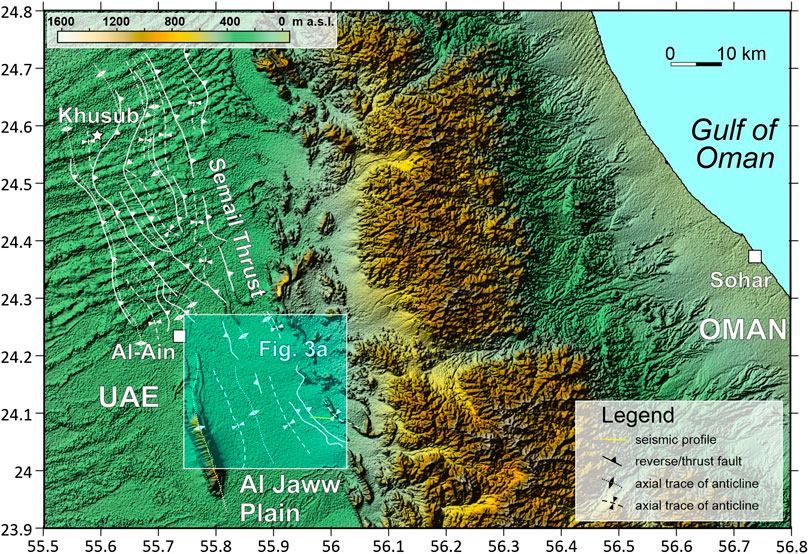
FIGURE 2. Digital terrain elevation. This data reveals the topographic pattern of Al Jaww Plain and surrounding areas, including the nearby Oman Mountains and the position of the ∼6-km long seismic profile, displayed to the right of the highlighted square showing the position of Figures 3A,B. The elevation data were acquired in February 2000 by the space shuttle Endeavour during the Shuttle Radar Topography Missions (SRTM), with a spatial resolution of 3 Arc-Second; they are freely downloadable form the USGS website (https://earthexplorer.usgs.gov). In white are drawn the main regional lineaments (as thrusts, sincline, and anticlane axial traces) that are found in the eastern Abu Dhabi Emirates by seismic and potential fields exploration (Woodward, 1994; Ali et al., 2008).

FIGURE 3

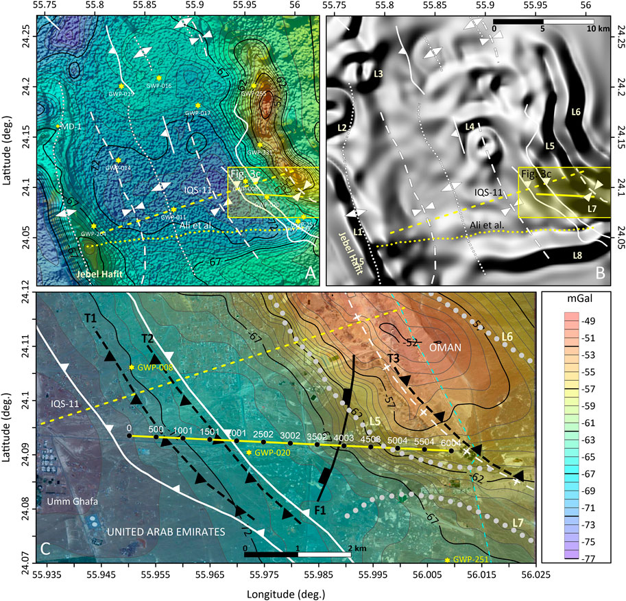
FIGURE 3. Maps of Al Jaww Plain. (A) Bouguer anomaly map (Ali et al., 2008). (B) Magnitude of the independent x- and y-component of local intensity gradients plotted using a gray-scale terrain representation based on Lambertian reflection. (C) Google Earth Image (^© CNES/Airbus and Maxar Technologies) with overlain the Bouguer anomaly and centered on the seismic profile (yellow line with metric progression). Symbols are as in Figure 2 except for gravimetric lineaments (light-green dotted lines) and surface inferred strike of the seismic faults (black dashed lines) in (C) and the main water boreholes in (A, C) (yellow stars).

In the adopted workflow, we first applied an edge detection technique to the high-resolution Bouguer anomaly map of Al Jaww Plain acquired by Ali et al. (2008). Our purpose was to locate the source boundary of Bouguer anomalies, comparing them with structural trends reported in the literature and with the results of our seismic interpretation. Precise delineation of tectonic structures is an essential basis for aquifer characterization, as faults and fractures have a strong influence on water distribution and mobility in the subsurface (e.g., Caine et al., 1996). Indeed, faults may behave both as barriers and conduits for fluid flow. Afterwards, we carried out a structural interpretation of the seismic profile locating the main subsurface tectonic structures and the major formation boundaries. Finally, to characterize the seismic properties of the subsurface, water-bearing formations in a wide depth range (i.e., from the near surface down to ∼1 km deep), the results from the coupled tomographic inversion of P velocity and Q factor were compared using a soft K-means clustering method, discussed in detail by Bernardinetti and Bruno (2019) and integrated with the interpretations from Prestack Depth Migration (PSDM) imaging.

When a seismic survey is designed for deep targets, e.g., a few kilometers, the imaging of the near surface can be a challenge (see, e.g., Pecholcs et al., 2002 and Vesnaver, 2004, among others). Single-source single-sensor surveys, also known as dense, wide aperture surveys, have been successfully used for many high-resolution studies of active faults and volcanic areas (e.g., Operto et al., 2004, Improta and Bruno, 2007, Bruno and Castiello, 2009, and Bruno et al., 2013), but only recently this field technique has been validated for large-scale 2D and 3D surveys (El-Emam and Khalil, 2012; Marmash et al., 2014; Granser et al., 2015). This recording geometry is appropriate for the tomographic imaging of direct and diving waves, provided that the local resolution of the Earth model to be inverted is consistent with the wavelength of recorded seismic waves (see, e.g., Berkhout, 1984 and Vesnaver and Böhm, 1997, among others). Bruno et al. (2010 and 2013) illustrated the advantage of the single-source single-receiver acquisition in terms of achieving a dense sampling of global source-receiver offsets for near-surface imaging by seismic reflection and first arrival tomography. In this paper, we rely on the high fold and global offset of direct and diving waves to invert not only for shallow velocities, as routinely carried out for tomostatic corrections (see, e.g., Zhu et al., 1992; Vesnaver et al., 2002; Zhang et al., 2006), but also jointly for the Q factor, as proposed by Böhm et al. (2006) and Rossi et al. (2007). Our implementation for the Q factor tomography relies on the frequency-shift method proposed by Quan and Harris (1997), but we adopted a new tool for estimating the frequency shifts without performing any spectral analysis of windowed waveforms (Vesnaver et al., 2020).

Hydro-Geological Setting

Al Jaww Plain is a westward sloping, low-relief alluvial piedmont located at the border with Oman that extends for approximately 550 km² (Figure 1). Rocks outcropping in the area have undergone complex compressional deformation. The eastern side of Al Jaww Plain is characterized by NNW-trending exposures of the allochthonous Semail Ophiolite and of the Hawasina Complex (Ali et al., 2008; Figure 1). These units are unconformably overlain by neo-autochthonous formations and by tertiary units (Searle and Ali, 2009), which were targeted by the seismic profile and will be discussed in detail in the following paragraphs. On the western side of the plain, the topographically prominent east-verging Jabal Hafit anticline exposes shallow-marine carbonates of Eocene to Miocene age in outcrop belts that trend parallel to the mountain range (Figure 1). According to Searle and Ali (2009), the east-verging Jabal Hafit fold is anomalous as it is antithetic to the dominant WSW vergence of other folds and WSW transport of thrusts in the area.

The plain development is strictly correlated to the Oman Mountains (Figure 2) that are formed as a result of two compressional events. The first occurred from the Late Cenomanian to the end of the Early Maastrichtian (Searle and Cox, 1999 and Searle, 2007) and involved the emplacement of a number of thrust sheets: each of them has been emplaced from NE to SW onto the Tethyan rifted continental margin of the Arabian Plate. Westward obduction of the Semail Ophiolite and its genetically related westward telescoping of the eastern Oman continental margin caused the loading and the down-flexing of the underlying autochthonous passive margin of shelf carbonates. The flexing resulted in the development of a foreland basin and a flexural bulge to the west of the obducted allochthons. The allochthons were intensely deformed, whereas the underlying Mesozoic shelf carbonates remained undeformed, except for minor extensional faulting associated with the flexural bulge (Boote et al., 1990 and Warburton et al., 1990).

A second compressional postobduction event occurred in the Late Eocene-Miocene during which the Arabian Plate moved north-eastwards and collided with the Eurasian Plate (Searle and Cox, 1999 and Searle, 2007). This collision produced large-scale folding, affecting both the Semail Ophiolite and the neo-autochthonous Maastrichtian and Paleogene cover and caused the reactivation of deep-seated faults in the frontal fold and thrust belt and in the adjacent foreland basin (Boote et al., 1990; Dunne et al., 1990; Searle et al., 1990). In addition, an uplift of at least 3,000 m occurred along the western flank of the northern Oman Mountains near the Al-Ain area (Boote et al., 1990). As a result of this uplift, the sedimentary successions were deeply eroded exposing (e.g., on Jabal Hafit) a full succession of Eocene-Miocene stratigraphy (Noweir, 2000), as described below.

The surface of Al Jaww piedmont plain is mostly covered with Quaternary sediments originated from the erosional dismantling of the Oman Mountains: they range from alluvial deposits, desert plain deposits, sabkha deposits, and aeolian sand. Surface drainage on the piedmont and alluvial fans subdivisions are canalized in wadies with variable flow patterns, exhibiting complexly braided channel morphologies (Menges et al., 1993). These unconsolidated sediments contain the largest reserves of fresh to slightly saline (i.e., 500–6,000 mg/L TDS: UN-ESCWA and BGR, 2013) groundwater in the Abu Dhabi Emirate, the Western Gravel Aquifer (WGA: Rizk and Alsharhan, 2008; Woodward, 1994). Its thickness ranges from 60 to 400 m, but is generally less than 150 m. Recharge to this generally unconfined aquifer, under present climatic conditions, results primarily from rainfall on the western flank of the Oman Mountains, which is rapidly transported westward toward the alluvial piedmont plain. This aquifer is heavily exploited in the Al Ain area (Al Shashi, 2002; El Mahmoudi, 2004; UN-ESCWA and BGR, 2013), where most of the extracted water is used for irrigation purposes. In 1985, about 95% of total water use in this area relied on it (Rizk and Alsharhan, 2008; Alsharhan et al., 2001). In 1993, the USGS and the Abu Dhabi National Drilling Company (NDC) started a groundwater research project, involving the drilling of more than one hundred wells. In many of them, petrophysical logs were performed (Al Shashi, 2002). In the Al Jaww plain, WGA permeability determined from those wells ranges from 2.9 × 10⁻⁴ to 4.6 × 10⁻³ m²/s. (UN-ESCWA and BGR, 2013).

In our test site, located to the west of the village of Umm Ghafa (Figure 3C), seismic and borehole data show that the aquifer is bounded at the bottom by the Miocene Fars Formation (Searle and Ali, 2009). It consists of continental clastic rocks, marine shale, and evaporitic rocks and is informally subdivided into the regionally recognized Upper Fars and Lower Fars Formations. A thick sequence of evaporite beds near the top of the Lower Fars forms a hydrogeologic confining unit, which keeps very saline groundwater in the Lower Fars separated from shallower fresh groundwater (Woodward, 1994). A regional unconformity divides the Fars Formation from the Oligocene limestones of the Asmari Formation (Cherif and El Deeb, 1984). Another regional unconformity separates it from an underlying thick and overall continuous sedimentary sequence made by the Mid-Upper Eocene limestones of the Dammam Formation by the anhydrites and dolomitized limestones of the Lower Eocene Rus Formation and by the Palaeocene marly limestones of the Umm Er Radhuma Formation (Searle and Ali, 2009). The abovementioned units unconformably overlie the Upper Cretaceous Fiqa Formation, which makes up most of the foreland basin sequence infill deposits and thickens toward the east (Ali et al., 2008).

The Dammam, the Rus, and the Umm er Radhuma formations host one of the major aquifer systems of the Arabian Peninsula: the “Umm er Radhuma-Dammam” Aquifer System (hereinafter indicated as URD) which extends from northern Iraq to the southern coast of the Arabian Peninsula over a distance of 2,200 km (UN-ESCWA and BGR, 2013). The total thickness of the aquifer system is only known in some areas. In the Jebel Hafit area, the aquifer system belongs to the confined-flow carbonate aquifer (Alsharhan et al., 2001). The Rus carbonates constitute an aquifer in the Al Ain region and are characterized by extensive dolomitization (Alsharhan et al., 2001). Other aquifers are located in the Umm er Radhuma and in Dammam formations (UN-ESCWA and BGR, 2013).

Significant variations in the lithostratigraphy of these three formations contribute to the complexity of the aquifer system, particularly the Rus, which is water-bearing in some areas, while it is acting as an aquitard in others. Permeability estimation from nuclear magnetic resonance in 72 rock samples from Rus, Dammam, and Asmari formations shows indeed a permeability range between 0.001 and 200 mD (Wampler et al., 2010). The Asmari formation has the greatest range in permeability, while the Dammam displays the greatest scatter. Data compiled by UN-ESCWA and BGR (2013) and based on Alsharhan et al. (2001) indicate an overall transmissivity of 3.6 × 10⁻⁵–6.5 × 10⁻⁵ m²/s for the Dammam aquifer. The Umm er Radhuma aquifer is instead characterized by an overall transmissivity range between 4.3 × 10⁻⁵ and 1.6 × 10⁻⁴ m²/s and a storativity of 9.0 × 10⁻⁴.

Fifteen bore-holes in the Jebel Hafit area produce about 7.7 MCM/year of groundwater from the Dammam Formation (Alsharhan et al., 2001). Because of its high radium and radon content, high temperature (36.5°C–51.4°C), and high salinity (3,900–6,900 mg/L TDS), this water is currently only used for recreational purposes. There are plans to use it for health and therapeutic purposes, as well as for the production of salt-tolerant crops.

Lineament Extraction from Gravity Anomaly

Exchange between the shallow and deeper, more saline, aquifers can occur at tectonically controlled, high-porosity, or high-permeability zones (Caine et al., 1996); therefore, a reliable location of tectonic features is important to assess movement and quality of groundwater in the Al Jaww Plain, and it is one of the main aims of this study. With this purpose, Woodward (1994) reprocessed and reinterpreted 33 seismic profiles in this area and proposed a structural map showing the major structural lineaments, including several shallow west-verging thrusts that affect the shallow aquifer system in the plain. Ali et al. (2008) acquired new gravity and magnetic profiles that were integrated with a new interpretation of an industry seismic reflection profile. This allowed them to propose an evolution of the sedimentary basin beneath the Al Jaww Plain. The outcomes of both Woodward (1994) and Ali et al. (2008) works are synthetized in the map of Figure 2, compared with our findings in Figure 3, and critically reviewed in this paper. It is worth noting that both Woodward (1994) and Ali et al. (2008) based their findings on the interpretation and modeling of 2D seismic, magnetic, and gravity profiles, while the high-resolution Bouguer anomaly, also produced by Ali et al. (2008), has not been directly used for tectonic feature recognition so far. Our first step of our data analysis was therefore to check if the strike and the position of the tectonic structures inferred in the Al Jaww Plain by Woodward (1994) and by Ali et al. (2008) are coherent with the high-resolution Bouguer anomaly map.

Gravity measurements for this map were collected using 416 stations spaced ∼1.0 km apart and covering an area of ∼500 km². The eastern side of the map is characterized by high-frequency gravity anomalies (≥−58.0 mGal) associated by Ali et al. (2008) with the thrusted Semail Ophiolite. The central area of Al Jaww Plain is characterized by strong low-gravity anomalies (≤−75.0 mGal), whereas the western area shows weaker positive anomalies (≥−70.0 mGal). Bouguer anomalies have a main NNW trend, which is coherent with the main strike of the subsurface thrusts and folds proposed by Woodward (1994) and by Ali et al. (2008). However, the gravity map also shows in the lower right sector a secondary but clear ENE trend, which does not correspond to any apparent tectonic structure discussed in the literature. The lack of ENE tectonic structures in this sector in the interpretations of Woodward (1994) and Ali et al. (2008) may occur because all 2D seismic and potential field profiles used by them are also ENE striking, and therefore not optimal to highlight ENE trends. With the aim of finding more solid hints about ENE tectonic lineaments, we processed the Bouguer anomaly map from Ali et al. (2008). Gravity is indeed a quite effective method for detecting subvertical geological features that might correspond to subsurface faults and contacts. Several techniques have been developed to analyze gravity anomalies produced by lineaments. Particularly interesting are those ones using edge-detection algorithms.

For our analysis, we adopted a MATLAB^® code for a gray scale, edge detection algorithm described by Canny (1986) and implemented by Wells (2013) and freely downloadable from the MATLAB Central File Exchange library. Canny edge-detection is a technique that extracts structural information from different vision objects. Moreover, it dramatically reduces the amount of data to be processed. In our implementation, first, we smoothed the Bouguer anomaly data matrix using a mean filter over a rectangle of size 4 × 4 (rows, columns) and converted the result into an intensity image matrix containing values in the range 0.0 (black) to 1.0 (white). Then, we computed the independent X- and Y-component of the local intensity gradient in the image using a derivative of Gaussian filter. Finally, both magnitude and direction of gradient were computed by taking, respectively, (1) the square root of the sum of squares and (2) the four-quadrant arctangent of the independent X- and Y-component of the local intensity gradient.

The standard implementation of this algorithm can also perform an automated edge tracking by hysteresis, which is based on an arbitrary definition of a threshold to determine potential edges. However, to avoid the loss of tiny but significant gravimetric features, we preferred to omit the edge tracking, and in Figure 3B, we show the whole magnitude map by a gray-scale terrain representation based on Lambertian reflection. In this map, NNW lineaments (labeled as L1, L5, and L6 in Figure 3B) as well as clear ENE trending lineaments (e.g., L2, L3, L7, and L8) and other minor circular features are apparent, the last ones probably related to the shape of the plain depocenter (L4) and/or to the interaction between NNW and ENE structures (L2, L3, and L7). Most of the lineaments evidenced in Figure 3B are likely to related to thrusts and dipping folds, having therefore a significant structural dip. Their gravimetric anomaly and gradient are also a function of their dip (Denit and Mudge, 2014). In presence of a significant structural dip, the maxima of the magnitude map, rather than highlighting the structure boundary (as for vertical features), will represent its expression at some depth, most likely closer to the surface, where the highest density contrast occurs. Modeling a structure dip from its gravimetric signature is difficult (e.g., Essa, 2013, and references therein). However, being able to estimate the structural dip from seismic data, we can assume that the magnitude maxima in Figure 3B will approximate the median point of the structure length, measured from surface to seismic basement (Gaudiosi et al., 2015).

By comparing the magnitude map with the terrain features and with the tectonic lineaments compiled from Woodward (1994) and Ali et al. (2008), we notice a good spatial correlation between the axis of Jabal Hafit anticline and lineament L1. Instead, the two high-magnitude, NNW-striking lineaments L5 and L6 cross-cutting the seismic profile do not overlap fairly well to any of east-verging structures of Woodward (1994) and Ali et al. (2008). Part of this error (∼4 km) can be due to structural dip as discussed above. Moreover, L5 and L6 show a light S-shaped curvature to the north, but not so pronounced as in Ali et al. (2008). Other NNW lineaments compiled from Woodward (1994) and Ali et al. (2008) do not have an evident gravimetric footprint, possibly meaning that such structures are minor local features below the resolution of available gravity data, which instead seemed to have a regional relevance is the ENE trending lineament L8, which could represent a transfer structure connecting the east-verging Semail and Hawasina thrusts (Figure 1). Another minor WNW-trending lineament labeled as L7 in Figure 3C could be originated at the contact between L5 and L8.

Seismic Field Experiment Description

The seismic survey was conducted at the southeastern boundary of the valley, along a roughly E-W line connecting Jabal Hafit with the northern Oman Mountains (Figure 3). The profile was acquired in November 2015 during the First EAGE Middle East Bootcamp, co-organized by the Petroleum Institute of Abu Dhabi (now part of Khalifa University), ADNOC (the Abu Dhabi National Oil Company), and Schlumberger through WesternGeco, which provided instrumentation and crew for the seismic profile acquisition. Profile location was designed to complement a nearly parallel legacy profile at a lower resolution and fold (i.e., line IQS-11 in Figure 3A) reprocessed by Woodward (1994). Moreover, the Bootcamp profile is almost parallel and shifted 4 km north of the eastern end of a gravimetric and magnetic profile acquired by Ali et al. (2008), see Figures 3A,B. Access restrictions did not allow us to follow a trend perfectly orthogonal to the mapped subsurface structures. Moreover, several small farms, water pumps, and a nearby road contributed to a relatively high level of noise in the seismic records (Figure 4A). Locations of known water wells are reported in Figures 3A,C. Figure 3C, zoomed on the seismic profile, shows that GWP-020 is the closest well to the seismic profile (near metric location 2,200). However, higher levels of disturbance from unknown sources are recorded between locations 3,750–4,172.

FIGURE 4

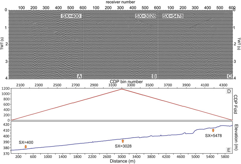
FIGURE 4. Seismic survey overview. Upper panel: three processed common shot gathers acquired with the source located at meters (A) 400, (B) 3,028, and (C) 5,478 (see red arrows in panel E). Lower Panels: (D) CDP fold coverage and (E) topographic pattern across the seismic profile.

The seismic line was acquired using a 600-channel array of vertical geophones with a natural frequency of 10 Hz covering the entire profile length of 6 km (Figure 4E). This spread allowed us to record reflection data characterized by a fold up to 1,200 traces in the CMP domain (Figure 4D), while spanning a variable range of maximum offsets along the survey, from 3 km at the center to 6 km at the extrema. Therefore, the recorded signals included near-offset near-vertical reflections, large-offset large-amplitude postcritical reflections, and deep-penetrating refracted waves, which are suitable for first arrival travel-time tomography, penetrating about 1–1.5 km deep. As our maximum offset is 6 km, we do not expect more than 1 km penetration from our picked first arrivals (i.e., about 1/4 to 1/5 of the maximum offset).

Seismic energy was provided by two ION AHV-IV Vibroseis used alternatively on different portions of the line to optimize the recording times. The sweeps ranged from 5 to 125 Hz with a duration of 21 s, for a total recording time of 27 s before correlation. The acquisition was carried out in two steps: in the first one, the receiver interval was set to 10 m; in the second one, a 5 m shift to the whole receiver array was applied, while repeating the vibration points at the same locations of the first step. In this way, we obtained a CMP spacing of 2.5 m. Further details are reported by Vesnaver et al. (2016).

Processing Sequence of Seismic Reflection Data

The reflection processing sequence was designed to exploit the densely spaced wide-aperture acquisition geometry, which provides multiangle reflections and better focuses the energy reflected from dipping reflectors, such as fault planes and steeply folded packages (Bruno et al., 2017 and Bruno et al., 2019). An exhaustive description of the data processing is beyond the scope of this paper; we present only the most important steps, whose details can be found in Yilmaz (2001) and references therein.

For comparison and quality control, we produced both conventional poststack and prestack depth migrated images (Figure 5). Both processing work flows aimed at preserving the relative amplitude relationships among reflectors. They included common steps (in black in Table 1), such as trace amplitude recovery, spiking and predictive deconvolution, and filtering, as well as different steps: in red are those related to Common-Midpoint processing (CMP) and in blue are those relative to the PSDM imaging. A basic processing step is the deconvolution, both spiking, which aims at improving the temporal resolution within the seismic reflection data and predictive which instead attempts to attenuate short-period multiples (Yilmaz, 2001). For both processes, we adopted a surface-consistent algorithm (Taner et al., 1981; Levin, 1989) that uses any combination of source, receiver, offset, and CMP components for power spectrum calculation and deconvolution.

FIGURE 5

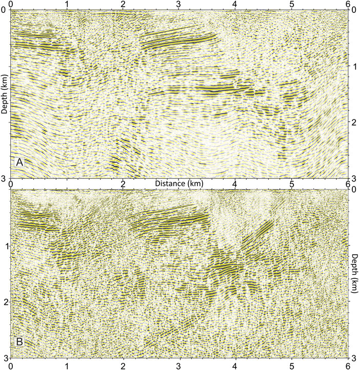
FIGURE 5. Seismic sections. Comparison between the depth migrated CMP stack (A) and the PSDM image (B). Both profiles are plotted with no vertical exaggeration and with a gradational yellow-white-black palette; positive amplitudes are in black.

TABLE 1

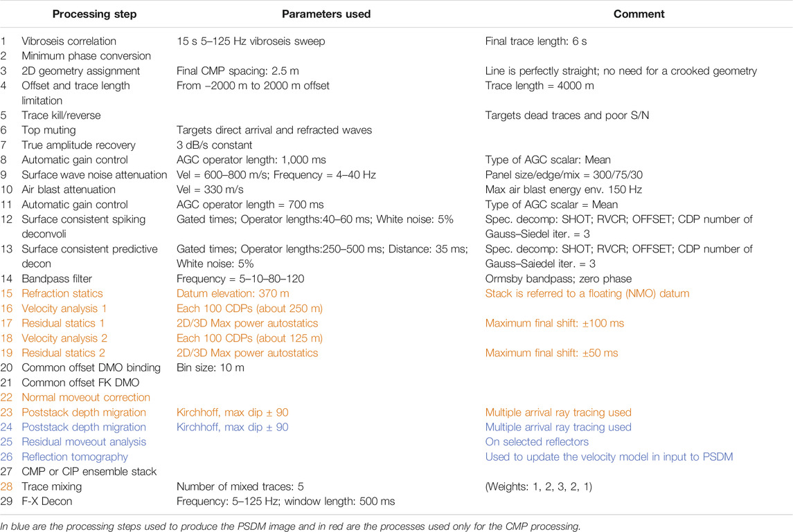
TABLE 1. Processing table. In black, the processes applied to both standard CMP and prestack depth migrated (PSDM) images are shown.

Another step in CMP processing is the RMS velocity estimation, which is needed for the normal-moveout correction and CMP stack. PSDM also needs a preliminary background velocity model to build a velocity model in depth. RMS velocity was estimated by picking the maxima of a semblance function (Neidell and Taner, 1971) computed across hyperbolic trajectories on selected CMP super-gathers. Super-gathers are composed of a few adjacent gathers, close enough that velocity differences among them are negligible. In this way, we gather more traces and offsets to compute the velocity spectra, reducing the noise contribution. The velocity models and the CMP stacks were refined by two cycles of residual statics corrections, followed by a further velocity analysis. For residual statics computation, we used the ProMAX SeisSpace ^® Maximum Power Autostatics algorithm, which is based on the method described by Ronen and Claerbout (1985).

CMP processing included the computation of near-surface refraction statics, which were applied before the velocity analysis phase. In arid onshore environments, where lateral velocity variations may be very sharp, surface-consistent refraction statics play indeed an important role for improving the quality of the stack (see Lawton (1989) and references therein). We picked the first arrival travel-times on the full-offset shot gathers. These travel times were used to estimate a high-frequency overburden/bedrock interface morphology and its velocity contrast by the Generalized Reciprocal Method refraction technique (Palmer, 1980). Seismic data were referenced to a floating datum, with an average altitude of 370 m a.s.l. First arrival picks are also used for the tomographic inversion, described later in this paper.

The PSDM algorithm we adopted does not require the application of refraction statics, as Kirchhoff migration is performed from topography in common offset domain. Migration from topography improves static corrections with respect to simple refraction statics, which are based on a vertical ray-path assumption. PSDM can overcome many of the typical drawbacks of CMP processing (e.g., Versteeg, 1993) because of its ability to focus reflectors within complex velocity distributions (see Figure 5). However, PSDM is highly sensitive to noise and to the accuracy of the velocity model, which is critical to account for the seismic wave propagation and ray-path bending in the depth domain. To build a reliable velocity model, we coupled PSDM with an iterative velocity building technique that also exploits reflection tomography in the poststack domain. Starting with the preliminary Vp model based on the semblance analysis, an initial PSDM run is performed to produce preliminary common image point panels, which are migrated trace ensembles generated by the PSDM. Reflection tomography is used to minimize the observed residual normal moveout and to update the velocity model. We iteratively assessed the quality of the velocity model by analyzing the flatness of reflected events on common image points (Guo and Fagin, 2002). We needed four iterations of PSDM, residual moveout picking and reflection tomography inversion to address complex nonlinear effects.

To improve the signal-to-noise ratio and to further increase the resolution, F-X deconvolution was applied to the migrated profiles of Figure 5. F-X deconvolution (Gulunay, 1986) applies a complex, unit-prediction Wiener filter along the spatial coordinate X for each frequency in the Fourier domain, and then inverse transforms each resulting trace back to its original domain, whichever it is, time or depth. This process reduces the random noise that often contaminates the input data.

The comparison between the poststack depth migrated and the PSDM sections is shown in Figure 5. We see that PSDM can better focus dipping reflectors, achieving an overall higher spatial resolution. For instance, in the PSDM image, we enhanced a west-dipping deep reflector with an apparent dip of 30°–45°, which we interpret as an east-verging thrust splay (T3 in Figure 6).

FIGURE 6

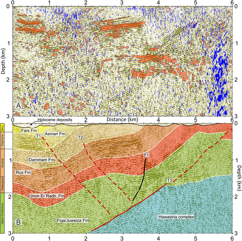
FIGURE 6. Seismic sections. PSDM seismic sections with superimposed the Energy (red) and Similarity (blue) attributes (A) and a structural interpretation (B). The energy attribute is a measure of reflectivity strength within the chosen depth-gate, while similarity is a multitrace attribute that returns trace-to-trace similarity properties. It ranges between 0 and 1: a similarity of 1 means that the trace segments are identical in waveform and amplitude. Similarity is the best indicator of structural discontinuity.

Structural Interpretation

The reflection characteristics of the stratigraphic and tectonic units depicted in our geological interpretation of Figure 6 are resumed in Table 2. For seismic facies classification, we used the technique described by Ramsayer (1979). Lacking available wells, our interpretation is based on comparison with a nearby seismic profile (also tied to an ∼800 m-deep water borehole) labeled as IQS-11 in Figure 3 and published by Woodward (1994), with the seismic and gravimetric and magnetic profiles of Ali et al. (2008) and of Searle and Ali (2009), on a geological cross-section shown by Searle and Ali (2009) across Jabal Hafit, which is located ∼16 km to the W of our profile and, finally, on the Late Cretaceous and Tertiary stratigraphy of the UAE-north Oman foreland along the SW flank of the Oman Mountains published by Nolan et al. (1990).

TABLE 2

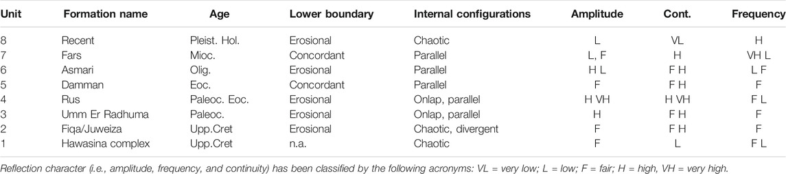
TABLE 2. Reflection characteristics of the stratigraphic and tectonic units depicted.

Based on these comparisons, we associate the upper 3-km thick reflective package laying above the base thrust, T3, to the neo-autochthonous Late Cretaceous to Paleogene sedimentary sequence (units 2–8 in Table 2). The uppermost seismic sequence is characterized by low-amplitude, high-frequency, and low-continuity reflector packages tied to the Miocene anhydrites of the Lower Fars Formation (Searle and Ali, 2009). The deepest stratigraphic unit above T3 is the Maastrichtian Fiqa formation, i.e., the base of the Upper Cretaceous foreland basin sequence (Searle and Ali, 2009). In particular, the Fiqa sequence displays a seismic reflection character that shows variable amplitude, continuity and frequency, and internal reflective configurations varying from parallel to sigmoid and chaotic/reflection free. This sequence is in tectonic contact, via T3, with an intensely deformed seismic basement, which is characterized by a chaotic reflection configuration and variable reflection character and has been interpreted as the Hawasina complex allochthonous (Searle, 2007), The seismic image shows that units above Hawasina are folded into a syncline, whose axial plane is located at about 0.8 km, and its eastern limb develops into an asymmetrical anticline bounded by the east-verging thrust T3. In our interpretation, the thrust develops at the bottom of the Fiqa Formation and separates it from the allochthonous Early Cretaceous Hawasina complex. Its base is not clearly visible in our data, due to the limited penetration depth achieved. The tentative upper continuation of T3 (dashed line in Figure 6) seems to develop within the Fiqa, intersecting the ground surface beyond the eastern end of the profile at a metric distance of ∼6,200 m–6,300 m. Two minor thrusts with opposite vergence (i.e., T1 and T2 in Figure 6) and with normal slips of 50 m–150 m, seem to terminate above T3. Their extrapolated trend intersects the surface at ∼580 m and ∼1750 m, respectively. A small-offset normal fault (F1) is also present in our interpretation between T2 and T3.

Figure 3C shows the inferred strike of T1, T2, and T3, constrained by literature data and by the results of the gravity boundary analysis, being separated by only 1 km The trend of the westernmost NNE-trending gravimetric lineaments “L5” is consistent with the strike of T3. If, in analogy with T3, L5 is a SW-dipping thrust and since the maximum of the boundary analysis will represent its expression at some depth, the spatial agreement between T3 and L5 is even better that what is pictured in the figure.

Concluding, our seismic interpretation of the seismic structure below Al Jaww Plain is consistent with gravity data and outlines a detachment fold and thrust above a basal detachment layer located at the base of the Fiqa Formation. Such interpretation is very similar to that provided by Warrak (1996) and Ali et al. (2008) for the nearby Jabal Hafit structure, and it is comparable to the interpreted seismic sections beneath the Jabal Hafit (Boote et al., 1990), which shows high-angle east-verging reverse faults that penetrate into the shelf carbonate sequence. It is worth noting that both Woodward (1994) and Ali et al. (2008) do not recognize east-verging structures in this area.

P-Velocity and Q-Factor Tomography

Our subsequent step was the geophysical characterization of the near-surface, i.e., down to about 750 m depth b.s.l. The area includes two aquifer systems: the unconfined WGA and the confined URD. Both aquifer systems have varying degrees of water saturation, salinity, and temperature. Two relevant parameters for modeling the fluid flow in porous media are the porosity and permeability of rocks, which must be estimated for a large 3D volume encompassing the saturated formation. Seismic refraction tomography (or the more expensive full-waveform inversion) can provide an accurate depth model for P-wave velocity, whose correlation with porosity and acoustic impedance is often satisfying (Wyllie et al., 1958; Raymer et al., 1980; Han et al., 1986; and Bangly et al., 1993, among many others). However, there is not a direct relationship between permeability and seismic velocity. The permeability is a very elusive parameter to estimate using a single seismic survey, unless the survey is repeated over time intervals using sophisticated time-lapse analysis tools. Looking for an alternative, we tested a coupled tomographic inversion of P velocity and Q factor. For this task, we picked and inverted the first arrivals, composed of direct, refracted, and diving waves. Part of the 2,376 available shot gathers was unusable for picking because of the high noise level. Initially, a manual picking was carried out interactively selecting one shot in ten, so a total of 169,397 first arrivals were picked manually. Later, this data was used as a seed for extending the interpretation to neighboring shot gathers using a neural-network first-break training and picking tool (e.g., Fahlman and Lebiere, 1990) included in the ProMAX SeisSpace^® processing suite. With this approach we were able to pick 287,873 traces, increasing the data density and the inversion reliability by 58%. However, differences between the two estimates are minor and so are not displayed. This similarity confirms the robustness of the processed data.

As the seismic source is a Vibroseis, we picked the peak of the symmetric Klauder wavelets originated during signal correlation. Attention must be paid to distinguish possible precursor lobes from the main one, but this problem arises mainly for later reflections (not considered here) and not much for the first arrivals we inverted for. It is however difficult to distinguish among the different seismic phases of the first arrivals, i.e., direct, refracted, and diving waves. In the inversion procedure, we assume that all of them are diving waves, relying on the minimum-time ray tracing algorithm embedded in the 3D tomographic algorithm we adopted (Rossi and Vesnaver, 2001). This algorithm converges automatically from this initially guessed phase to other phases (as reflected, refracted, or direct), if needed, by fitting the velocity field during the tomographic inversion (Böhm et al., 1999).

The quality of the tomographic images depends tightly on the picking accuracy. Uncertainty on travel time readings ranges from 2.5 ms (i.e., 1/8 of the dominant period of the P-pulse) to 10–12 ms, depending on data quality and offset. As mispicks can provide travel times that are both larger and smaller than the actual ones, often they mutually compensate, bringing the average uncertainty 4 ms, when the total number of picked signals is large, as in our case. This is proven by the fact that the inversion of our initial set of 169,397 events provided results comparable to those obtained from the expanded set of 287,873 events.

Inversion Procedure

For both travel time and Q factor tomography, we used the Cat3D software (Böhm et al., 1999) and in particular the staggered-grid approach (Vesnaver and Böhm, 2000). This method is particularly robust with respect to the noise and reduces the inversion ambiguities. For the Q factor estimation, we adopted the approach described by Quan and Harris (1997) and Rossi et al. (2007), i.e., taking a time window centered around the picked travel time and computing the spectral centroid of the extracted waveform. This works well for strong events without interferences, but it becomes challenging for noisy vibroseis signals, where weaker signals may be confused with the lateral ripples of a Klauder wavelet. For this reason, we tested an alternative approach based on the envelope and instantaneous frequency attributes for evaluating the spectral centroid, based on the theoretical work of Saha (1987) and Poggiagliolmi and Vesnaver (2014). In brief, for an ideal zero-phase Vibroseis signal, i.e., a Klauder wavelet, the travel time is picked at the waveform peak, which fits the envelope maximum. Precisely, at that point, the instantaneous frequency is evaluated and used for the spectral centroid calculation; thus, there is an automatic perfect match between the propagation time used for estimating P-wave velocity and anelastic absorption. For a minimum-phase signal, instead, a minor mismatch occurs because the signal time break must be used for the velocity inversion, while the envelope maximum has a small delay with respect to it. However, except for very small travel times, i.e., for early arrivals at short offsets, such a difference is definitely negligible. The results originated using the two different approaches were very similar and therefore are not displayed separately. However, the human involvement with the second approach was much lower, in terms of both personal interpretation and man-hours, so resulting in a cost-effective, unbiased alternative (Vesnaver et al., 2020).

To reduce the dependence of diving-wave inversion from the initial model (Vesnaver, 2004), a multiscale inversion flow was adopted (Figure 7). The basic assumption is that large wavelength anomalies in the velocity structure have a dominant amplitude relative to the smaller ones (e.g., De Landro et al., 2017), which is reasonable. In a multiscale approach, the horizontal resolution is very low initially, to get a stable estimation of the low spatial frequencies and the vertical velocity trend. The output of each step is divided into smaller pixels and used as an initial model for a higher resolution inversion. The model scaling continues until we approximate the maximum resolution that is consistent with the seismic signal. As the maximum frequency of first arrivals is ∼100 Hz and their average velocity is ∼2 km/s, the minimum wavelength is ∼20 m. We assumed this value as our resolution limit, both laterally and vertically. The histogram of travel time residuals computed for the final, small-wavelength model shows a tighter distribution centered at zero with respect to those computed for the large-wavelengths, confirming that the adopted multiscale strategy was efficient in exploring the multidimensional model parameter space.

FIGURE 7

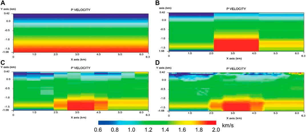
FIGURE 7. Multiscale tomographic inversion. The resolution is constant vertically, but increases laterally in sequence: (A) only 1 voxel; (B) 3 voxels; (C) 9 voxels; (D) 100 voxels.

The first initial model is composed of 30 homogeneous horizontal layers with a thickness of 70 m and a velocity increasing linearly from 0.5 to 2 km/s. Similarly, the Q factor is increasing linearly from 5 to 500. The chosen ranges are wider than what we actually expected to reduce the footprint of the “a priori” information over the inversion outcome, as we prefer as much as possible a data-driven solution. We carried out the tomographic inversion by a full 3D algorithm, to allow minor deviations of the profile from a straight line and a few off-line shot points.

The first 1D inversion (Figure 7A) provides a velocity of about 2 km/s (dark blue) in the shallowest 200 m and a high velocity of 5 km/s at the bottom of the model. Splitting the layers into three voxels (Figure 7B), lateral variations are spotted, i.e., a shallow velocity increase from West to East (where the outcropping ophiolites are located). A central anomaly with high velocity shows up at a depth of 1.2 km. When increasing the voxel number to 10 and 100 (Figures 7C,D), two distinct low-velocity anomalies are visible, with the larger and thicker one on the central and deeper part of the model. A tiny and shallow high-velocity anomaly also shows up in the proximity of the eastern end of the profile. The ray path of diving waves at the last iteration in Figure 7 is much denser in the upper 500 m than elsewhere and almost missing below 1 km. For this reason, we plotted the estimated P velocity and Q factor by blanking the deeper parts with ray coverage lower than 10 ray segments per pixel (Figures 8, 9).

FIGURE 8

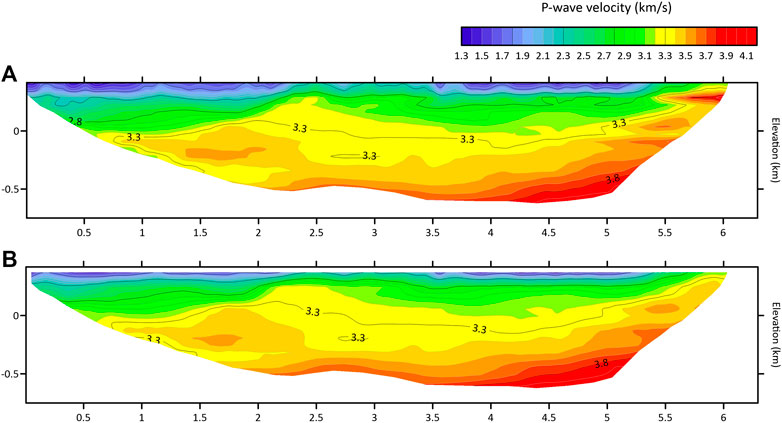
FIGURE 8. Tomographic resolution. Comparison between the tomographic high-resolution (i.e., 315 × 105 nodes) P-wave velocity model (A) and the low-resolution (i.e., 63 × 21 nodes) P-wave velocity model (B). The areas with a low ray coverage are blank.

FIGURE 9

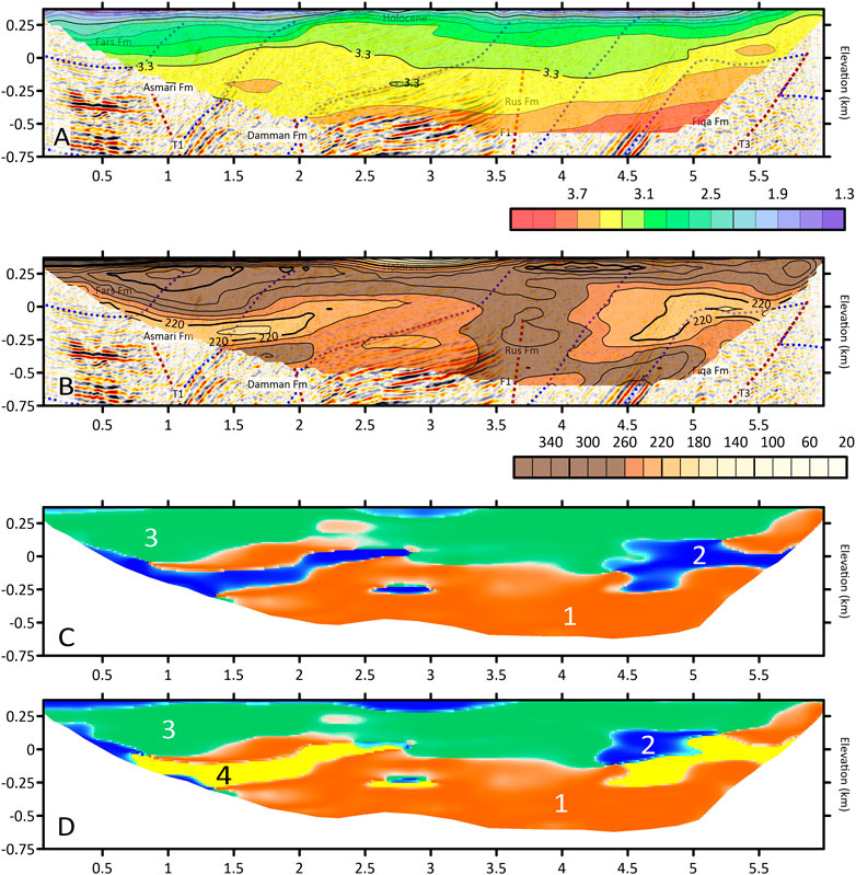
FIGURE 9. P-velocity and Q-factor information. Tomographic images of P velocity (A) and Q factor (B), as in Figure 9, overlain to the PSDM seismic section of Figure 5B. Depth is limited to an elevation of −750 m a.s.l. Blue dots show interpreted formation limits, and dark red dashed line show the tectonic lines as in Figure 6. (C, D) show the results of the K-means clustering with three and four clusters, respectively.

Figure 8 compares the high-resolution P-wave velocity (A) tomographic model (i.e., 315 × 105 nodes; 20 × 20 m cell) with a lower-resolution model (63 × 21 nodes; 100 × 100 m cell) which we will later use for the K-means clustering with the Q factor. The reason of this choice is to achieve overall the same penetration in depth, which for the high-resolution model of Q factor is limited, and to speed-up the computations. Also, the lower resolution achieves some smoothing of the velocity field, which enhances the results of the prestack depth migration. Comparison between the high-resolution (A) and the low-resolution P-wave velocity models shows that not only the loss in small wavelengths (and therefore in detail) affects the shallow part of the model but also the main features are retained by the lower resolution model, except for the shallow high-velocity anomaly at about 6 km distance in Figure 8A. The higher-resolution P-wave model overall better details small-wavelength features of the very shallow low-velocity zone which can delineate the top of the WGA, as its velocity is lower than 1.5 km/s. Similar features occur for the estimated Q factor too.

While the P-wave velocity estimated by tomography is an absolute value, the Q factor is a relative contrast, which needs an independent calibration to be directly comparable among surveys with different recording instruments, ideally by borehole measurements (Vesnaver et al., 2020). Such a calibration is not available for our survey; thus, we pay attention mainly to the relative spatial variation of the estimated Q factor.

The ideal tool to quantify the tomographic inversion reliability is the Singular Value Decomposition (SVD) of the tomographic matrix (e.g., van der Sluis and van der Vorst, 1987, among many others). From the singular values we can compute both a global quality parameter, as the condition number, or even a local measure of inversion ambiguity in the estimated Earth model, as the null-space energy (Vesnaver, 1994; Vesnaver, 1996). However, the computational cost of SVD is comparable to the inversion of a full matrix nxn, where in our case n is equal to 169,397 or 287,873. This size exceeds the computing power available to us and to most other people. Thus, we limited our uncertainty estimation by adopting the much cheaper ray density, i.e., the number of ray segments that cross a given voxel in the tomographic grid. Although such an indicator is not rigorous, it is an acceptable approximation of SVD in most cases.

Subsurface Rock Characterization

In Figure 9, the P-velocity and Q-factor models are overlain to the PSDM seismic image and its interpretation to facilitate the comparison. For hydrogeological interpretations, the link between P velocity, Q factor, and reflectivity is relevant, since in layered and fractured rocks the seismic wave propagation and attenuation is macroscopically affected by changes in porosity and fracture density at the mesoscopic scale (Shapiro and Mueller, 1999; Rubino and Hollinger, 2012). The Q factor is more sensitive than P velocity to porosity variations: theoretical and experimental works show that the Q factor decreases with increasing porosity (e.g., McRae and Zala, 1995; Jeanne et al., 2014). Figure 9 shows that both the P-velocity and Q-factor trends are affected by the stratigraphic and tectonic settings, but, as expected, variations are more evident in the Q-factor estimate.

In detail, we notice a 1-km-wide and ∼100-m-thick near-surface high P-wave anomaly centered at 3 km distance and matching the outcrops of the stiff carbonates of Dammam formation (Figure 6B). This high P-wave anomaly is associated with a low Q-factor, probably due to fracturing or karsting. Except for this anomalous low Q-factor shallow zone, the Q factor is higher (>260) in the upper part of the model, down to ∼0 m a.s.l. (∼370 m depth) over the entire profile. Below this thick high-Q zone, two areas at lower Q factor are separated by a subvertical, ∼1-km-wide high Q-factor anomaly, extending over the entire model depth, and centered at 3.75 km. The western low-Q anomaly shows a more complex trend with two minima. The upper one is located within the limestones of the Asmari and upper Dammam Formations. The second lower and smaller minimum is instead in the topmost, less reflective part of Rus Formation. Both the western low-Q anomalies have patterns that are hardly following the stratigraphic contacts. The easternmost Q factor minimum is more uniform, and its pattern follows more closely the stratigraphic trend, in particular the high-amplitude high-dip reflective package found across the Palaeocene marly limestones of the Umm Er Radhuma and the topmost part of Fiqa Formations. The subvertical high-Q area separating the eastern and western low-Q anomalies is almost entirely located within the low-porosity anhydrites and dolomitized limestones of the Rus Formation and above the fault F1. Due to its overall low reflectivity and similarity (Figure 6A), this area may be interpreted as a large fault damage zone. Here, combination of lithology and tectonics could overall act as a barrier for water circulation. We remark that the P-velocity model does not show any macroscopic evidence for this vertical high-Q anomaly. Moreover, the P-wave model shows very little lateral variations in the areas with highest Q factor variation, with only two small high P-wave anomalies roughly matching the minima of the two wider and more complex western and eastern Q-factor anomalies.

The P-wave velocity estimated by first-arrival tomography had to be smoothed, to avoid instabilities and artefacts that arise in the migration algorithm when sharp velocity variations occur. Also, in the deeper part not crossed by diving waves, we integrated the tomographic information by conventional migration velocity analysis, i.e., by flattening Common Image Gathers (see, e.g., Yilmaz, 2001). The latter procedure can easily handle velocity inversions, if present. This is possible because of the ray tracing algorithm embedded in the travel time inversion that we adopted, based on the minimum-time and bending approach (Rossi and Vesnaver, 2001). Indeed, a few shallow velocity inversions show up in the high-resolution tomographic velocity field in Figure 8A.

K-Means Clustering

Petrophysical characterization of rock samples from the carbonate formations is imaged in the seismic profile and outcropping around the study area point at significant variations of porosity (e.g., Ali et al., 2008 and Searle and Ali, 2009 and references therein). It is reasonable to think that those variations, together with other factors, (1) macroscopically affect the estimated P velocity and Q factor (e.g., Shapiro and Mueller, 1999; Rubino and Hollinger, 2012) and (2) can be enhanced by clustering techniques applied to Vp and Q factor. From the analysis of Figures 9A,B, the Q factor seems more sensitive to lithological and/or porosity variations than P velocity. To better analyze subtle relationship between P velocity and Q factor, we used an unsupervized learning method based on the K-means clustering (Lloyd, 1982), a well-known partitional, nonhierarchical, and unsupervised algorithm, which allows dividing a dataset into “K” clusters based on distances among points. The algorithm minimizes the variance within each cluster and maximizes that one among different clusters.

For our dataset, we used a soft K-means approach discussed by Bernardinetti and Bruno (2019) that links the silhouette index to the pixel color saturation. The silhouette index (Rawashdeh and Ralescu, 2012) compares the distances of every ith observation within a cluster with the average extracluster distances. In other words, the silhouette index measures the degree of confidence in the clustering assignment of a given observation. Silhouette Index ranges from −1 to 1. In our color palette, values less than 0, which are typical of misclustered observations, are represented in white. Clusters with values of the silhouette index very close to 0, which highlights observations with unclear assignment, are mapped with light colors. With this simple technique, transactions among clusters are so graphically rendered as color changes (see Figures 9C,D). With respect to the typical hard clustering algorithms, this gradational color scheme allows to readily locate areas where observations are well/poorly clustered and spot local dissimilarities and transition zones.

Additionally, the silhouette index provides a statistical criterion to evaluate the optimal number of clusters K, which is arbitrary in the standard implementation of the K-means algorithm. Determining the optimal number of clusters for a dataset is a fundamental issue in partitioning clustering. According to Kaufman and Rousseeuw (1990), the optimal number of clusters K is the one that maximizes the average silhouette index over a range of possible K values. However, the optimal number of clusters is somehow subjective and depends on the method used for measuring similarities and on the parameters used for partitioning. For our dataset, the average silhouette index in Figure 10A suggests an optimal cluster number of 3, which corresponds to the spatial cluster distribution of Figure 9C. However, average silhouette index is also high for K = 4, which instead corresponds to the spatial cluster distribution of Figure 9D in both cases (i.e., K = 3 and K = 4); the cluster assignment is robust, since the respective silhouette indexes in Figure 10B are characterized by very few negative/small numbers. This is also well-represented by the color palettes of the two models of Figures 9C,D.

FIGURE 10

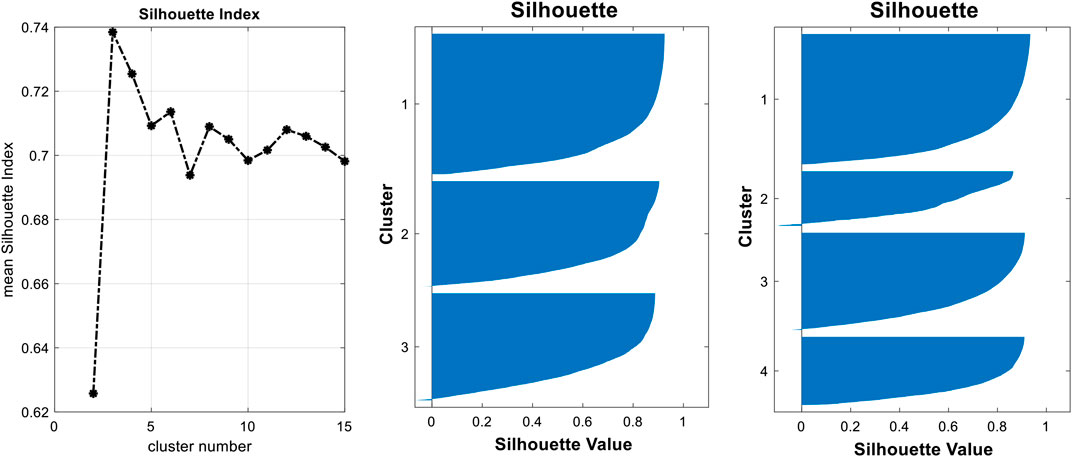
FIGURE 10. (A) Silhouette analysis. Average silhouette index obtained varying the number of clusters from 2 to 15. The optimal clustering was found at the maximum value for k = 3. (B, C) show the graphical silhouette values for each class of the K-means runs with k = 3 and k = 4.

Even if the 3-class clustering has a slightly higher average silhouette index, it does not allow discriminating fairly well between low-Vp and high-Vp (Figure 11), while the scatterplots of P velocity (Vp) vs. Q factor (Figure 11) show that a 4-class classification is more useful for rock characterization, since it allows partitioning the (Vp, Q) observations in four domains: (1) high-Vp and high-Q; (2) low-Vp and low-Q; (3) low-Vp and high-Q; and (4) high-Vp and low-Q. Compared with the 3-class clustering, the 4-class clustering roughly splits cluster 2 of Figure 9C into clusters 2 (i.e., low-Vp and low Q) and 4 (i.e., high-Vp and low Q) in Figure 9D. In particular, low-Vp and low-Q zones mapped to cluster 2 (blue) might suggest a higher likelihood of presence of water-saturated high-porosity porous rocks with respect to the high-Vp and low-Q zones mapped to cluster 4 (yellow). Such information is neither evident nor simple to extract by a simple visual comparison of the P-wave and Q-factor models of Figures 9A,B.

FIGURE 11

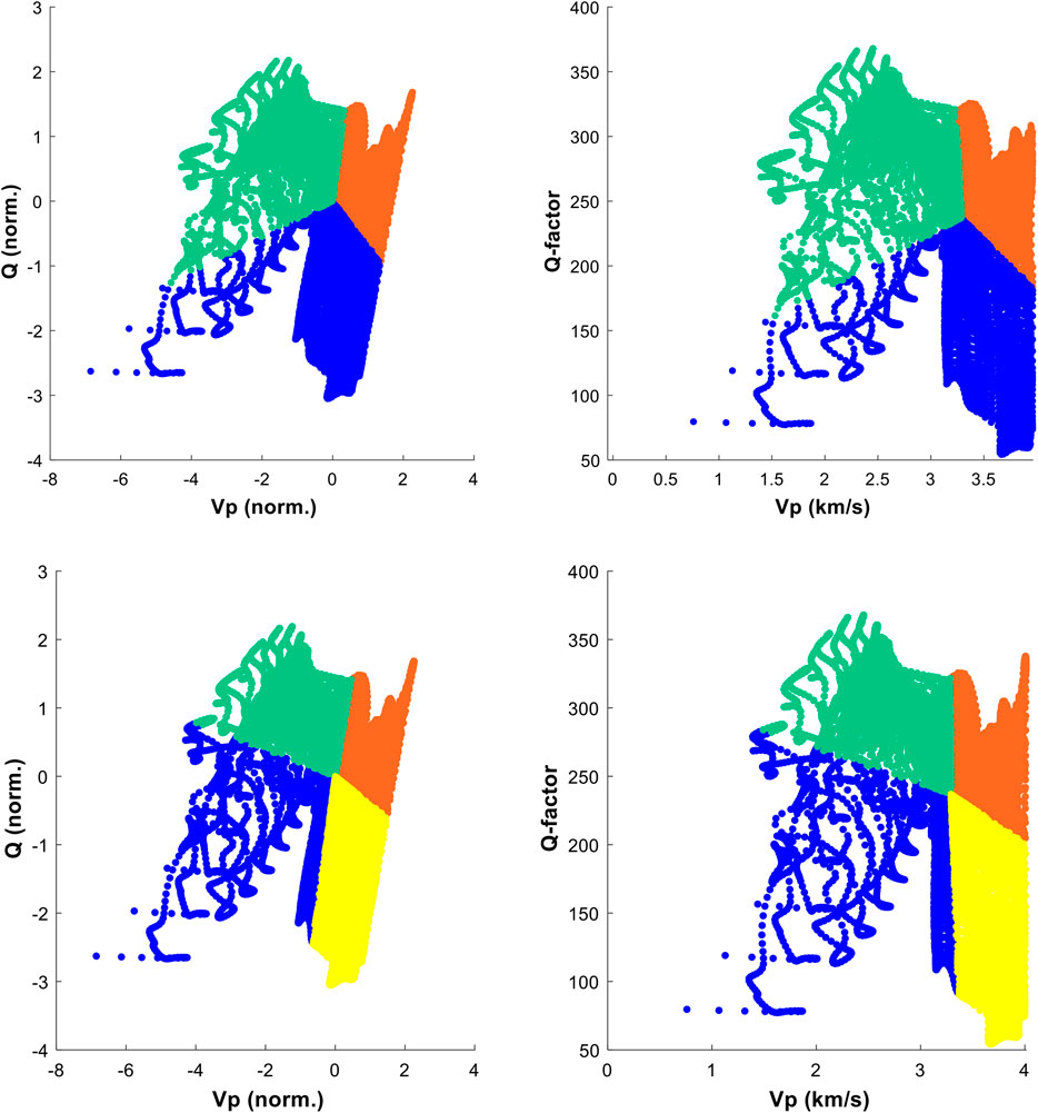
FIGURE 11. Scatterplots. Scatterplots of the bivariate dataset (P velocity and Q factor) before (right) and after normalization (left). Colors are scaled as in Figure 9 and display the classification of the cloud of points obtained with the K-mean clustering with three clusters (upper graphs) and four clusters (lower graphs).

Discussion

Figure 12 shows the 4-class K-means model overlain to the geological interpretation of the seismic reflection profile, which provides a reliable structural and stratigraphic background to interpret the results of the K-means clustering. Considering that the subsurface rocks are mainly carbonates with a different degree of porosity and within and above them there are reported evidences of different aquifer systems (i.e., WGA: Rizk and Alsharhan, 2008; URD: Alsharhan et al., 2001), low P-wave and low-Q zones mapped to cluster 2 may represent an estimation of the maximum likelihood of the presence of water-saturated porous rocks in the subsurface rock formations. Less promising, but still interesting, are the zones of cluster 4 (yellow), with low Q and high Vp, which might be related to stiffer fractured rocks with a lower water saturation.

FIGURE 12

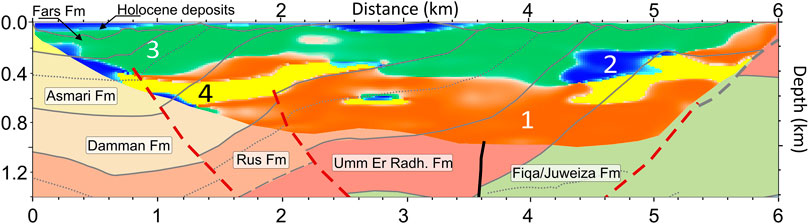
FIGURE 12. Interpretation vs. clusters. Spatial distribution of the clusters overlain to the geological interpretation from the seismic reflection images of Figure 6.

The figure shows that, within the overburden, a tiny layer of cluster 2 (blue color) is visible throughout the western half of the profile from 0 to 3.8 km (see also Figure 9D). This layer thickens in two sectors located at the western end of the section (between 0 and 1 km) and in the central of part the section (2.3–3.6 km), while it disappears after 4 km. The low-permeability anhydrites of the Lower Asmari Formation, which outcrops between 1 and 2 km, may play a role in decreasing the thickness of cluster 2. Overall, cluster 2 has an average thickness of about 40 m–60 m, reaching a maximum of 120 m and a minimum value of 20 m (i.e., one pixel) at 1.2 km. Its near-surface distribution 2 well agrees with location of the WGA. This aquifer is under production, as pumping occurs in several wells located along the seismic profile.

Three USGS-NDC wells are close to the seismic profile (Figure 3). Well GWP-20 (Figure 3) almost crosses it, being located at about 200 m to the south and at about 2.2 km distance (Figures 9D, 12). This well reaches a depth of 232 m, and in 1990, the measured aquifer thickness was 88.1 m, with a static water level found at 18.6 m b.g.l. (USGS-NDC, 1993; Al Shahi, 2002). A measured specific conductance of 2,400 μS/cm indicates a fairly good water quality with a relatively high level of salinity. Well GWP-020 underwent a pumping test on May 20, 1990, performed with a pumping rate of 14.8 m³/h for 6 h. The drawdown was 77.8 m indicating a (low) specific capacity of 0.190 m³/h. Considering that, since 1990, the water level has dropped at least 20 m–30 m (Al Shahi, 2002), and taking into account the resolution limit of the K-means analysis (i.e., 20 × 20 m), the actual estimated thickness of the aquifer is in agreement with our results, which show around GWP-020 a cluster 2 thickness of about 40 m.

The other two wells are a bit too distant from the seismic line to allow a reliable correlation: GWP-008 is about 1.2 km to the north of the western end of the seismic profile. It was drilled for 732 m, and in 1990, both aquifer thickness and water table level were comparable to those of GWP-20 (USGS-NDC, 1993; Al Shahi, 2002). Neither conductance measurements nor pumping tests were performed in this well.

Well GWP-251 is instead located nearly 1.2 km to the south of the eastern end of the line. It was drilled for 340 m and both a lithological description and petrophysical logs are published in El Mahmoudi (2004). The Quaternary overburden, made of gravel and sand, is 95 m thick in this area. The water level here drops at 55 m b.g.l. and specific conductance in the aquifer ranges between 6,000 and 7,200 mS/cm, indicating a lower water quality with respect to GWP-020. A 15-m-thick layer of low-permeability claystone separates the unconfined WGA from a sequence of limestones and mudstones that, according to our seismic interpretation, should belong to the Umm Er Radhuma formation. Taking into account the 2-km offset between this well and the seismic profile and a further water table drop since 1990, lithological and hydrological data well correlate with P-wave velocity and Q-factor and with their integrated K-means analysis. Such analysis shows that cluster 2 is missing in this area, suggesting a shrinking or even disappearing of the WGA toward the east, as indicated by the well.

Taking into account the previous discussion, we assume that other potentially water-saturated areas (i.e., confined aquifers) might be highlighted by the presence of cluster 2 in deeper carbonate formations in the western, central, and eastern sectors of the 2D K-means model, down to a maximum depth of about 600 m b.s.l. These areas might denote deeper, more saline water reserves of the URD aquifer system (Alsharhan et al., 2001; UN-ESCWA and BGR, 2013). It is worth recalling here that, in Al Ain area nearly 7.7 MCM/year of high temperature (36.5°C–51.4°C) and high salinity (3,900–6,900 mg/L TDS) groundwater is pumped from the Dammam Formation.

Interpretation of the westernmost part of the K-means model is less robust being very close to the model boundary. It shows that cluster 2 splits into two sectors: a shallower one located within the lower Fars and the upper Asmari Formations. A tiny deeper area is instead located at about 600 m deep, within the limestones of lower Asmari and upper Dammam Formations. Two small, laterally elongated cluster two zones are also present in the central part of the section (∼3 km), respectively, at ∼0 and 0.6 km deep. They are located within the limestones of Asmari and Dammam Formation, respectively, and the shape of the deeper cluster seems to be influenced by the stratigraphic trend (here, the stratigraphic contact between Dammam and Rus Formation is also affecting the boundary between cluster 4 and 1). Finally, the largest potentially water-saturated zone is found in the eastern part of the section, within the Palaeocene marly limestones of the Umm Er Radhuma and in the upper part of Fiqa Formations. It has an average thickness of more than 200 m and a lateral extension of ∼800 m.

Conclusion

Groundwater assessment and monitoring is a central task in arid countries where water constitutes an important element for sustainable development. For such task the integration of multivariate data (nowadays widely applied for oil exploration) helps reducing the interpretation risk and provides a consistent and unbiased (i.e., objective) geophysical background for further studies. This paper discusses a multivariate approach aimed at geophysical characterization of subsurface rocks, which can provide qualitative yet useful hints for groundwater exploration in arid environments. It integrates, at different scales and resolution, gravity data with seismic reflection images; P-velocity and Q-factor tomography from a novel seismic profile was acquired in the framework of the First EAGE Middle-East BootCamp. We present both a reliable geo-structural framework and an estimation of the location of water-saturated porous rocks in the subsurface of Al Jaww Plain.

First, edge-detection techniques applied to the Bouguer anomaly map produced by Ali et al. (2008) allowed us to confirm presence of NNW structural trends reported by Woodward (1994) and by Ali et al. (2008) and suggest as unreported ENE structural strikes, and the main one was localized to the south of the study area and was interpreted as a transfer zone connecting the east-verging Semail and Hawasin thrusts. Since tectonic structures can effectively influence groundwater flow and provide a path for shallow pollutants to seep into deeper aquifers, their location is an essential base for aquifer characterization and protection.

Subsequent analysis, based on data from the new seismic survey, provided useful information for a more detailed subsurface rock characterization. The PSDM image showed a strong a west-dipping deep reflector, consistent with gravity data which we interpret as an east-verging thrust splay affecting seismic ray propagation. This structure, not known in the previous literature, allowed us to interpret the subsurface of Al Jaww Plain as a detachment fold and thrust above the base of the Fiqa Formation, similarly to Jabel Hafit structure. The reflectivity image provided us with an earth model that is consistent with the available geophysical and geological information and allowed us to better interpret the results of the coupled inversion of P velocity and Q factor.

In layered and fractured rocks, seismic wave propagation and attenuation are macroscopically affected by changes in porosity and fracture density at the mesoscopic scale (Shapiro and Mueller, 1999; Rubino and Hollinger, 2012), and our field results are consistent with their findings. Both theoretical and experimental works (e.g., McRae and Zala, 1995; Jeanne et al., 2014) show that the Q factor decreases for increasing porosity, which is more sensitive than P-wave velocity to porosity variations. Mapping the spatial variation of those parameters along a cross-section can provide consequently a qualitative estimation of the water saturation or porosity in sedimentary porous rocks. However, P velocity and Q factor are influenced also by other petrophysical parameters; therefore, a simple correlation between Q factor or between P-wave velocity and rock porosity and fluid saturation is not feasible.

We used an unsupervised learning method based on the K-means clustering, to better analyze subtle relationships between P-wave velocity and Q factor and possibly highlight the presence of water-saturated porous rocks in the subsurface. Using this approach, we were able to spot areas characterized by low values of P velocity and low values of Q factor, which may be a geophysical clue for high-porosity, water-saturated rocks in the subsurface. We remark that further key parameters from petrophysical logs and electric resistivity data are needed for a better hydrological characterization of the subsurface. Once available, they can be integrated in the proposed workflow. Nevertheless, our results show that, by analyzing all available information that can be extracted by a standard, active seismic experiment, one can reduce the number of wells and optimize their location resulting in reduced exploration cost.

Data Availability Statement

The raw data supporting the conclusions of this article will be made available by the authors, without undue reservation.

Author Contributions

PB processed and interpreted the seismic reflection data, performed the K-means analysis, prepared most of the figures, and wrote the preliminary manuscript. AV performed first-arrival analysis and took care of the tomographic inversion of P-wave velocity and Q factor. Both authors were equally involved in the field data acquisition and manuscript editing/reviewing.

Funding

This work was supported by internal funds of ADNOC (Abu Dhabi National Oil Company), EAGE (European Association of Geoscientists and Engineers), and Schlumberger.

Conflict of Interest

The authors declare that the research was conducted in the absence of any commercial or financial relationships that could be construed as a potential conflict of interest.

Acknowledgments

The authors thank EAGE (European Association of Geoscientists and Engineers) for co-organizing the First EAGE Middle-East BootCamp, together with other former colleagues of the Khalifa University of Science and Technology, and our student Jing Yeob Na, who cared the travel time picking. In particular, we thank Asha Alia and Raymond Cahill (EAGE) for their valuable support. We thank the main sponsor, Western-Geco Schlumberger, especially Ismail Haggag, David Morrison, and Bruno Vermeulen, and the other sponsors, i.e., ADNOC, OMV, and Mubadala. Processing of seismic reflection data has been performed using SeisSpace^® ProMAX^® software. The authors acknowledge support of this work via a Landmark Grant Program to INGV and to the University of Napoli ‘Federico II’ by Halliburton Software and Services, a Halliburton Company.

References

Ali, M. Y., Fairhead, J. D., Green, C. M., and Noufal, A. (2017). Basement structure of the United Arab Emirates derived from an analysis of regional gravity and aeromagnetic database. Tectonophysics 712, 503–522. doi:10.1016/j.tecto.2017.06.006

CrossRef Full Text | Google Scholar

Ali, M. Y., Sirat, M., and Small, J. (2008). Geophysical investigation of Al Jaww plain, eastern Abu Dhabi: implications for structure and evolution of the frontal fold belts of Oman Mountains. GeoArabia 13, 91.

Google Scholar

Al Lazki, A. I., Seber, D., Sandvol, E., and Barazangi, M. (2002). A crustal transect across Oman Mountains on the eastern margin of Arabia. GeoArabia 7, 47–78.

Google Scholar

Al Shahi, F. A. (2002). Assessment of groundwater resources in selected areas of Al Ain in the UAE. Master thesis, UAEmirates University. https://scholarworks.uaeu.ac.ae/all_theses/96.

Google Scholar

Alsharhan, A. S., Rizk, Z. A., Nairn, A. E. M., Bakhit, D. W., et al. (2001). Hydrogeology of an arid region: the Arabian Gulf and Adjoining areas. 1st Edn. Amsterdam/New York: Elsevier.

Google Scholar

Berkhout, A. (1984). Seismic resolution: a quantitative analysis of resolving power of acoustical echo techniques. Benahavis, Spain: Geophysical Press, 228.

CrossRef Full Text | Google Scholar

Bernardinetti, S., and Bruno, P. P. G. (2019). The hydrothermal system of solfatara crater (Campi Flegrei, Italy) inferred from machine learning algorithms. Front. Earth Sci 7, 286. doi:10.3389/feart.2019.00286

CrossRef Full Text | Google Scholar

Blangy, J. P., Strandeness, S., Moos, D., and Nur, A. (1993). Ultrasonic velocities in sands—revisited. Geophysics 58, 344–356. 10.1190/1.1443418

CrossRef Full Text | Google Scholar

Böhm, G., Accaino, F., Rossi, G., and Tinivella, U. (2006). Tomographic joint inversion of first arrivals in a real case from Saudi Arabia. Geophys. Prospect 54, 721–730. doi:10.1111/j.1365-2478.2006.00563.x

Google Scholar

Böhm, G., Rossi, G., and Vesnaver, A. (1999). Minimum-time ray tracing for 3D irregular grids. J. Seismic Explor 8, 117–131.

CrossRef Full Text | Google Scholar

Boote, D. R. D., Mou, D., and Waite, R. I. (1990). “Structural evolution of the Suneinah Foreland, Central Oman Mountains,” in The geology and tectonics of the Oman region. Editors A. H. F. Robertson, M. P. Searle, and A. C. Ries (London, UK: Geological Society of London, Special Publication no.) Vol. 49, 397–418.

CrossRef Full Text | Google Scholar

Bradford, J. H., and Sawyer, D. S. (2002). Depth characterization of shallow aquifers with seismic reflection, Part II – Prestack depth migration and field examples. Geophysics 67, 98–109. doi:10.1190/1.1451372

PubMed Abstract | CrossRef Full Text | Google Scholar

Bruno, P. P. G., Berti, C., and Pazzaglia, F. J. (2019). Accommodation, slip inversion and segmentation in a province-scale shear zone from high-resolution, densely spaced, wide-aperture seismic profiling, Centennial Valley, MT, USA. Sci. Rep. 9, 9214. doi:10.1038/s41598-019-45497-1

CrossRef Full Text | Google Scholar

Bruno, P. P. G., DuRoss, C. B., and Kokkalas, S. (2017). High-resolution seismic profiling reveals faulting associated with the 1934 Ms 6.6 Hansel Valley earthquake (Utah, USA). Geol. Soc. Am. Bull. 129, 1227–1240. doi:10.1130/B31516.1

CrossRef Full Text | Google Scholar

Caine, J. S., Evans, J. P., and Forster, C. B. (1996). Fault zone architecture and permeability structure. Geology 24 (11), 1025–1028. doi:10.1130/0091-7613(1996)024<1025:fzaaps>2.3.co;2

CrossRef Full Text | Google Scholar

Canny, J. A. (1986). Computational approach to edge detection. IEEE Trans. Patt. Anal. Machine Intell., PAMI 8 (6), 679–698. 10.1109/TPAMI.1986.4767851

Google Scholar

Carcione, J. M. (2014). Wave fields in real media. Theory and numerical simulation of wave propagation in anisotropic, anelastic, porous and electromagnetic media. 3rd Edn. Amsterdam, NL: Elsevier, 690.

CrossRef Full Text | Google Scholar

Cassiani, G., Böhm, G., Vesnaver, A., and Nicolich, R. (1998). A geostatistical framework for incorporating seismic tomography auxiliary data into hydraulic conductivity estimation. J. Hydrol 206, 58–74. doi:10.1016/S0022-1694(98)00084-5

CrossRef Full Text | Google Scholar

Cherif, O. H., and El Deeb, W. M. Z. (1984). The Middle Eocene-Oligocene of the northern Hafit area, south of Al Ain City (United Arab Emirates). Geologie Mediterr 11, 207–217. doi:10.3406/geolm.1984.1310

PubMed Abstract | CrossRef Full Text | Google Scholar

De Landro, G., Serlenga, V., Russo, G., Amoroso, O., Festa, G., Bruno, P. P., et al. 3D ultra-high-resolution seismic imaging of shallow Solfatara crater in Campi Flegrei (Italy): new insights on deep hydrothermal fluid circulation processes. Sci. Rep. 7, 3412 (2017). doi:10.1038/s41598-017-03604-0

CrossRef Full Text | Google Scholar

Dentith, M., and Mudge, S. T. (2014). Geophysics for the mineral exploration geoscientist. Cambridge, UK: Cambridge University Press, 516.

Google Scholar

Dunne, L. A., Manoogian, P. R., and Pierini, D. F. (1990). “Structural style and domains of the northern Oman Mountains (Oman and United Arab Emirates),” in The geology and tectonics of the Oman region. A. H. F. Robertson, M. P. Searle, and A. C. Ries London, UK: Geological Society of London, Special Publication no., Vol. 49, 375–386.

Google Scholar

El Mahmoudi, A. (2004). Geophysical and hydrogeological investigations of the quaternary aquifer at Al Jaww Plain, Al Ain area. Fast Co 9 (1), 17–28.

CrossRef Full Text | Google Scholar

El-Emam, A., and Khalil, S. (2012). “Maximizing the value of single-sensor measurements, Kuwait experience,” in SEG annual meeting, 4-9 November 2012, Las Vegas, 1–5 [Expanded abstracts].

Google Scholar

Essa, K. S. (2013). Gravity interpretation of dipping faults using the variance analysis method. J. Geophys. Eng 10, 015003. 10.1088/1742-2132/10/1/015003

CrossRef Full Text | Google Scholar

Gaudiosi, G., Nappi, R., Alessio, G., Porfido, S., Cella, F., Fedi, M., et al. (2015). “Integrated analysis of seismological, gravimetric and structural data for identification of active faults geometries in Abruzzo and Molise areas (Italy),” in EGU general assembly, Vienna, April 12–17, 2015 [abstract].

CrossRef Full Text | Google Scholar

Granser, H., Novotny, B., Fava, L., and Vermeulen, B. (2015). “Recent 4S high-fold 3D seismic acquisition in the Abu Dhabi foreland of Oman Mountains,” in ADIPEC conference, [Expanded abstracts], SPE-177534-MS. doi:10.2118/177534-MS

CrossRef Full Text | Google Scholar

Gulunay, N. (1986). “F-X decon and the complex Wiener prediction filter for random noise reduction on stacked data.” in 56th SEG annual meeting. 2-6 November 1986, Houston [Expanded abstracts], POS 2.10. doi:10.1190/1.1893128

Google Scholar

Guo, N., and Fagin, S. (2002). Becoming effective velocity-model builders and depth imagers, part 2: the basics of velocity-model building, examples, and discussion. Lead. Edge 21, 1210–1216. 10.1190/1.1536136

CrossRef Full Text | Google Scholar

Han, D., Nur, A., and Morgan, D. (1986). Effects of porosity and clay content on wave velocities in sandstones. Geophysics 51, 2093–2107. 10.1190/1.1442062

CrossRef Full Text | Google Scholar

Improta, L., and Bruno, P. P. (2007). Combining seismic reflection with multifold wide‐aperture profiling: an effective strategy for high‐resolution shallow imaging of active faults. Geophys. Res. Lett 34, L20310. 10.1029/2007GL031893

CrossRef Full Text | Google Scholar

Kaufman, L., and Rousseeuw, P. J. (1990). Finding groups in data: an introduction to cluster analysis. John Wiley & Sons, 342.

CrossRef Full Text | Google Scholar

Lawton, D. C. (1989). Computation of refraction static corrections using first-break traveltime differences. Geophysics 54, 1289–1296. doi:10.1190/1.1442588

Google Scholar

Levin, S. A. (1989). Surface-consistent deconvolution: Geophysics 54, 1123–1133. doi:10.1190/1.1442747

Google Scholar

Lloyd, S. (1982). Least squares quantization in PCM. IEEE Trans. Inf. Theor 28, 129–137. doi:10.1109/TIT.1982.1056489

CrossRef Full Text | Google Scholar

Marmash, S., Al Jenaibi, M. A., Al Jeelani, O. S., Haggag, I. B., Morrison, D., and Glushchenko, A. (2014). “Case history – the first S4 survey in Abu Dhabi,” in ADIPEC conference [Expanded abstracts], SPE-171829-MS.

CrossRef Full Text | Google Scholar

Mavko, G., Mukerji, T., and Dvorkin, J. (1998). The rock physics handbook: tools for seismic analysis in porous media. Cambridge, UK: Cambridge University Press, 329.

CrossRef Full Text | Google Scholar

Menges, C. M., Hadley, D. G., Woodward, D. G., and Mohamed, F. A. (1993). Geology and geophysics, groundwater resources of Al-Ain area, Abu Dhabi Emirate,” in US geological survey administration, Vancouver, USA, Rep. 93–001, 74–167.

CrossRef Full Text | Google Scholar

Miller, R. D., Pullan, S. E., Waldner, J. S., and Haeni, F. P. (1986). Field comparison of shallow seismic sources. Geophysics 51, 2067–2092. doi:10.1190/1.1442061

CrossRef Full Text | Google Scholar

Neidell, N. S., and Taner, M. T. (1971). Semblance and other coherency measures for multichannel data. Geophysics 36, 482–497. doi:10.1190/1.1440186

CrossRef Full Text | Google Scholar

Nieto, D., Baradello, L., Accaino, F., Böhm, G., Madrussani, G., and Vesnaver, A. (2014). Aquifer characterization and monitoring by active and passive seismic surveys. Procedia Eng. 89, 1231–1234. doi:10.1016/j.proeng.2014.11.425

CrossRef Full Text | Google Scholar

Noweir, M. A. (2000). Back-thrust origin of the Hafit structure, northern Oman Mountain Front, United Arab Emirates. GeoArabia 5 (2), 215–228.

Google Scholar

Operto, S., Ravaut, C., Improta, L., Virieux, J., Herrero, A., and Dell’Aversana, P. (2004). Quantitative imaging of complex structures from dense wide‐aperture seismic data by multiscale traveltime and waveform inversions: a case study Geophys. Prospect 52, 625–651. doi:10.1111/j.1365-2478.2004.00452.x

CrossRef Full Text | Google Scholar

Palmer, D.. (1980). The Generalized reciprocal method of seismic refraction interpretation. Tulsa, Ok: Society of Exploration Geophysicists.

Google Scholar

Pecholcs, P., Hastings-James, R., Barsoukov, N., and Al-Ramadan, A. (2002). “Universal land acquisition 14 years later,” in SEG annual meeting, 6-11 October 2002, Salt Lake City, 56–59 [Expanded abstracts].

CrossRef Full Text | Google Scholar

Poggiagliolmi, E., and Vesnaver, A. (2014). Instantaneous phase and frequency derived without user-defined parameters. Geophys. J. Int. 199, 1544–1533. doi:10.1093/gji/ggu352

CrossRef Full Text | Google Scholar

Prasad, M., Zimmer, M. A., Berge, P. A., and Bonner, B. P. (2005). Laboratory measurements of velocity and attenuation in sediments,” in Near-surface geophysics. Editor D. K. Butler, 491–502, Tulsa, USA: SEG, 732 pp.

CrossRef Full Text | Google Scholar

Quan, Y., and Harris, J. M. (1997). Seismic attenuation tomography using the frequency shift method. Geophysics 62, 895–905. doi:10.1190/1.1444197

Google Scholar

Ramsayer, G. R. (1979). “Seismic stratigraphy, a fundamental exploration tool,” in Offshore technology conference.

Google Scholar

Rawashdeh, M., and Ralescu, A. (2012). Crisp and fuzzy cluster validity: generalized intra-inter silhouette index” in Fuzzy information processing society (NAFIPS), 2012 annual meeting of the North American, 6-8 August 2012, (Berkeley, USA: IEEE), 1–6.

CrossRef Full Text | Google Scholar

Raymer, L. L., Hunt, E. R., and Gardner, J. S. (1980). “An improved sonic transit time-to-porosity transform,” in Transactions SPWLA, 21st annual logging symposium, 8-11 July 1980, Lafayette, USA, P1–P13.

Google Scholar

Rizk, Z. A., and Alsharhan, A. S. (2008). Water resources in the United Arab Emirates. Amman: Ethraa Publishing.

CrossRef Full Text | Google Scholar

Ronen, J., and Claerbout, J. F. (1985). Surface-consistent residual statics estimation by stack-power maximization. Geophysics 50, 2759–2767. doi:10.1190/1.1441896

CrossRef Full Text | Google Scholar

Rossi, G., and Vesnaver, A. (2001). Joint 3D traveltime inversion of P. S and converted waves. J. Comput. Acoust. 9, 1407–1416. doi:10.1016/S0218-396X(01)00149-2

CrossRef Full Text | Google Scholar

Rossi, G., Gei, D., Böhm, G., Madrussani, G., and Carcione, J. M. (2007). Attenuation tomography: an application to gas-hydrate and free-gas detection. Geophys. Prospect 55, 655–669. doi:10.1111/j.1365-2478.2007.00646.x

Google Scholar

Saha, J. G. (1987). “Relationship between Fourier and instantaneous frequency,” in SEG annual meeting, 11-15 October 1987, New Orleans, USA, 591–594 [Expanded abstracts].

Google Scholar

Searle, M. P. (2007). Structural geometry, style and timing of deformation in the Hawasina Window, Al Jabal al Akhdar and Saih Hatat culminations, Oman Mountains. GeoArabia 12, 99–130.

CrossRef Full Text | Google Scholar

Searle, M. P., and Cox, J. S. (1999). Tectonic setting, origin and obduction of the Oman ophiolite. Geol. Soc. Am. Bull. 111, 104–122. doi:10.1130/0016-7606(1999)111<0104:TSOAOO>2.3.CO;2

CrossRef Full Text | Google Scholar

Searle, M. P., and Ali, M. Y. (2009). Structural and tectonic evolution of the Jabal Sumeini – Al Ain – Buraimi region, northern Oman and eastern United Arab Emirates. GeoArabia 14, 115–142.

CrossRef Full Text | Google Scholar

Searle, M. P., Cooper, D. J. W., and Watts, K. F. (1990). Structure of the Jebel Sumeini-Jebel Ghawil area, Northern Oman,” in The geology and tectonics of the Oman region. Editors A. H. F. Robertson, M. P. Searle, and A. C. Ries (London, UK: Geological Society of London, Special Publication), Vol. 49, 361–374.

Google Scholar

Shapiro, S. A., and Mueller, T. M. (1999). Seismic signature of permeability in heterogeneous porous media. Geophysics 64, 99–103. doi:10.1190/1.1444536

CrossRef Full Text | Google Scholar

Taner, M. T., Koehler, F., and Sheriff, R. E. (1981). Surface consistent corrections. Geophysics 46, 17–22. doi:10.1190/1.1441133

CrossRef Full Text | Google Scholar

UN-ESCWA and BGR (2013). Inventory of shared water resources in western Asia. Beirut: United Nations Publications, 606.

CrossRef Full Text | Google Scholar

van der Sluis, A., and van der Vorst, H. A. (1987). Numerical solution of large, sparse linear algebraic systems arising from tomographic problems.” in Seismic tomography. Seismology and exploration geophysics 5. Editor G. Nolet (Dordrecht: Springer).

Google Scholar

Versteeg, R. J. (1993). Sensitivity of prestack depth migration to the velocity model. Geophysics 58, 873–882. doi:10.1190/1.1443471

CrossRef Full Text | Google Scholar

Vesnaver, A. (1996). The contribution of reflected, refracted and transmitted waves to seismic tomography: a tutorial. First Break 14, 159–168. doi:10.3997/1365-2397.1996010

Google Scholar

Vesnaver, A. (2004). The near-surface information gap for time and depth imaging. Geophys. Prospect 52, 653–661. doi:10.1111/j.1365-2478.2004.00445.x

CrossRef Full Text | Google Scholar

Vesnaver, A. (1994). Towards the uniqueness of tomographic inversion solutions. J. Seismic Explor 3, 323–334.

CrossRef Full Text | Google Scholar

Vesnaver, A., and Böhm, G. (1997). Physical criteria for adaptive seismic tomography. SEG Tech. Prog. Expan. Abstr. 1997, 1448–1451. doi:10.1190/1.1885684

Google Scholar

Vesnaver, A., and Böhm, G. (2000). Staggered or adapted grids for seismic tomography? Lead. Edge 19, 944–950. doi:10.1190/1.1438762

CrossRef Full Text | Google Scholar

Vesnaver, A., Böhm, G., Cance, P., Dal Cin, M., and Gei, D. (2020). Windowless Q-factor tomography by the instantaneous frequency. Geophys. Prospect 68, 2611–2636. doi:10.1111/1365-2478.13020

CrossRef Full Text | Google Scholar

Vesnaver, A., Bridle, R., German, J., Hu, L., Kim, J. J., Ley, R., et al. (2002). “Tomostatics for half a million traces,” in SEG annual meeting, 957–960. [Expanded abstracts].

CrossRef Full Text | Google Scholar

Vesnaver, A., Iqbal, M., Bouzidi, Y., Bruno, P. P., and Ali, M. Y. (2016). “First results from the EAGE Middle-East BootCamp seismic survey in the Jebel Hafeet area,” in ADIPEC conference [Expanded abstracts]. SPE-183276-MS. doi:10.2118/183276-MS

Google Scholar

Wampler, J. J., Sondergeld, C. H., and Rai, C. S. (2010). “Estimating permeability in UAE carbonates using NMR,” in SEG annual meeting, 2649–2653 [Expanded abstracts].

CrossRef Full Text | Google Scholar

Warburton, J., Burnhill, T. J., Graham, R. H., and Isaac, K. P. (1990). The evolution of the Oman Mountains foreland basin,” in The geology and tectonics of the Oman region. Editors A. H. F. Robertson, M. P. Searle, and A. C. Ries (London, UK: Geological Society of London, Special Publication), Vol. 49, 419–427.

Google Scholar

Warrak, M. (1996). Origin of the Hafit structure: implications for timing the tertiary deformation in the northern Oman Mountains. J. Struct. Geol. 18, 803–818. doi:10.1016/S0191-8141(96)80014-9

CrossRef Full Text | Google Scholar

Wells, J. R. D. (2013). Grayscale Canny edge detection, MATLAB central file exchange. https://www.mathworks.com/matlabcentral/fileexchange/52956-grayscale-canny-edge-detection. (Accessed May 25, 2020).

Google Scholar

Whiteley, R. J., Hunter, J. A., Pullan, S. E., and Nutalaya, P. (1998). “Optimum offset” seismic reflection mapping of shallow aquifers near Bangkok, Thailand. Geophysics 63, 1385–1394. doi:10.1190/1.1444440

CrossRef Full Text | Google Scholar

Woodward, D. (1994). Contributions to a shallow aquifer study by reprocessed seismic sections from petroleum exploration surveys, eastern Abu Dhabi, United Arab Emirates. J. Appl. Geophys. 31, 271–289. doi:10.1016/0926-9851(94)90062-0

CrossRef Full Text | Google Scholar

Wyllie, M. R. J., Gregory, A. R., and Gardner, G. H. F. (1958). An experimental investigation of factors affecting elastic wave velocities in porous media. Geophysics 23, 459–493. doi:10.1190/1.1438493

CrossRef Full Text | Google Scholar

Yilmaz, O. (2001). “Seismic data analysis (2 volumes),” in SEG, Tulsa, USA, investigations in geophysics. Vol. 10, 1000.

Google Scholar

Zhu, X., Sixta, D. P., and Angstman, B. (1992). Tomostatics: turning‐ray tomography + static corrections. Lead. Edge 11 (12), 15–23. doi:10.1190/1.1436864

CrossRef Full Text | Google Scholar