Recovering the Effects of Subgrid Heterogeneity in Simulations of Radionuclide Transport Through Fractured Media

1. Introduction

Understanding the fate and migration of dissolved contaminants is important for practical applications such as the optimal design of aquifer remediation strategies (Bolster et al., 2009), the delineation of protection areas around wells used for drinking water production (Trinchero et al., 2008) or the safety assessment of a repository for spent nuclear fuel (SKB, 2010).

Contaminant transport depends on the groundwater flow velocity field and this is in turn affected by the underlying heterogeneous distribution of hydraulic conductivity. Fully characterizing this distribution is impossible and thus upscaled macrodispersion models are typically used (Gelhar and Axness, 1983). However, these models are only valid for mild to low degrees of heterogeneity, whereas natural sedimentary aquifers often exhibit variations of up to 12 orders of magnitude in hydraulic conductivity (Bear, 1972; Sanchez-Vila et al., 2006). This requires the use of alternative upscaling methods (Hakoun et al., 2019).

In fractured crystalline rocks, transport patterns are particularly complex as they depend on both the topological configuration of the sparse network of fractures (network-scale heterogeneity) and the variable distribution of fracture openings (fracture-scale heterogeneity). Moreover, a large volume of these fractured systems that is not affected by fluid flow is still accessible by solutes via a mechanism called matrix diffusion (Neretnieks, 1980). The coupling between solute advection along the open conductive fractures and diffusion into the rock matrix is a function of the underlying groundwater flow velocity field. It turns out that a proper characterization of groundwater velocity patterns is crucial to properly simulate contaminant transport (along conductive fractures) and retention (in the intact rock matrix).

An appealing approach for simulating groundwater flow and advective transport in fractured media is by means of Discrete Fracture Network (DFN) models (Cacas et al., 1990). DFN models account for the structural heterogeneity of the site, by means of field-derived statistical properties, and could also include fracture internal heterogeneity (Makedonska et al., 2016). In these models, contaminant retention in the rock matrix can be accounted for by using time domain particle tracking calculations (Painter et al., 2008).

Despite being methodologically attractive, DFN models are computationally challenging and sometimes simplifications are required, particularly when multiple stochastic realisations must be assessed. These simplifications are often carried out at the expense of a careful characterization of the local groundwater flow velocity field. Hence, methods to reconstruct the underlying variability of groundwater velocity are required. In particular it is important to recast the significant spatial persistence of high/low velocity regions along connected fractures, which was observed in previous works (Benke and Painter, 2003; Painter and Cvetkovic, 2005; Comolli et al., 2019; Hakoun et al., 2019). Different approaches have been proposed to represent that persistence (e.g., Benke and Painter, 2003; Painter and Cvetkovic, 2005; Comolli et al., 2019; Hakoun et al., 2019). Although these approaches differ in operational details, they are all based on some type of spatial Markov approximation for the Lagrangian velocity. This means that spatial persistence in velocity is simulated by assuming that the underlying Lagrangian velocity is a spatial Markov process, which implies that velocity in one fracture segment depends only on the velocity of the preceding segment.

A few approaches have been proposed to extrapolate or reconstruct velocity fluctuations, and related travel times, in large-scale DFN models. For instance, recently Hyman et al., 2019 have shown that heavy-tailed first passage time distributions can be reproduced using time domain random walk simulations based on transition times between fracture intersections. In Hyman et al., 2019 velocity variations within fractures are neglected and statistical ergodicity is invoked to sample velocity from a parametric distribution. The approach is shown to reproduce well the tail of a first passage time distribution but it is inadequate to describe the abrupt rising limb caused by early arrivals, which are mostly controlled by few large and transmissive fractures and are thus clearly not ergodic. A similar approach was presented earlier by Painter and Cvetkovic, 2005 to extrapolate velocity distributions from small-scale to much larger-scale DFN models. The main difference is that in the method by Painter and Cvetkovic, 2005 empirical distribution functions of the velocity field are derived from DFN models statistically representative of the large-scale fracture intensity, orientation and distribution. Therefore, the method is suited to reproduce the full travel time distribution and not only the tail.

Here, the algorithm of Painter and Cvetkovic, 2005 is used to reconstruct the lost variability in velocity by means of stochastic simulations. The proposed approach is used in combination with a computationally challenging DFN model of a Brittle Fault Zone (BFZ). In the DFN models used to assess the safety of proposed sites for geological repositories of spent nuclear fuel in fractured crystalline rock, the representation of BFZ is a topic of particular attention, due to the importance of such zones in determining site-scale flow and transport pathways (Hartley et al., 2018).

Radionuclide transport calculations are here carried out using particle tracking in the time domain (Painter et al., 2008). That and closely related approaches have been used in combination with discrete fracture networks in previous studies related to safety of geological disposal options (e.g., Selroos and Painter, 2012; Poteri et al., 2014; Trinchero et al., 2016, 2020), radionuclide transport at contaminated sites (Kwicklis et al., 2019), and production of natural gas from unconventional reservoirs (Karra et al., 2015). The focus here is on stochastic approaches to recover the transport effects of the subgrid velocity variability that is lost when using upscaled representations of fracture swarms associated with BFZs in large-scale flow models. In particular, we evaluate and refine the transport downscaling algorithm of Painter and Cvetkovic, 2005. All the radionuclide transport calculations are carried out using the computer code MARFA (Painter et al., 2008; Painter and Mancillas, 2013).

2. Methods

2.1. Representation of Brittle Fault Zones as Fracture Swarms

Structurally, BFZ typically consist of a damage zone with finite thickness, containing many small fractures, about a central fault core (Aaltonen et al., 2016). Many BFZ are hydraulically active, and extend for multiple kilometres, providing hydraulic connectivity over long ranges with significant implications for the safety of geological repositories for spent nuclear fuel. In the groundwater flow and transport modeling calculations performed for repository safety assessments, the most commonly used approach has historically been to represent each BFZ as either a large planar fracture (in a DFN model) or a homogeneous volume (in a continuum model). This is the approach adopted in the previous generation of site descriptive modeling studies by both the Swedish (Joyce et al., 2010) and Finnish (Posiva, 2013) radioactive waste management organisations. In the DFN case, both stochastic variability and depth-dependency of flow and transport properties has sometimes been assigned to the plane using a relatively simple scaling-law formulation, relating transmissivity to fracture size, together with a normally-distributed random component, as in Joyce et al. (2010).

In the most recent iteration of the Olkiluoto DFN Version 3 (ODFN3) model, describing the site of the repository currently under construction in Finland, a new representation of BFZ was developed (Hartley et al., 2018). In this formulation, BFZ damage zones are explicitly modeled as finite-thickness swarms of fractures stochastically generated around each fault core. Three-dimensional heterogeneity of the flow field within a zone can therefore be simulated, with effects such as choking of flow included. While this is a major advance, the added realism of this description comes at a computational cost. Methods for simplifying this BFZ model, while retaining heterogeneity in flow and transport properties, are desirable for the large number of particle tracking simulations required for a safety assessment calculation. This study therefore investigates several such methods by applying them to a simple test DFN model and comparing the results of flow and transport simulations.

2.2. Discrete Fracture Network Model of a Single Brittle Fault Zone

A simplified DFN model, consisting of a single BFZ fracture swarm overlaying a randomly oriented background fracture network is used as the basis of these simulations. Parameters are chosen to match a typical BFZ in the Olkiluoto DFN Version 3 (ODFN3) model (Hartley et al., 2018). One stochastic realization of the BFZ fracture swarm component of this model is shown in subfigure A of Figure 1.

FIGURE 1

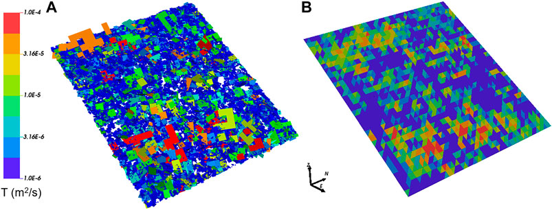
FIGURE 1. Comparison of BFZ representations; (A) is a single realization of the underlying DFN model; (B) is the plane-projected representation of the same realization. Fractures colored by transmissivity.

The BFZ fracture swarm is stochastically generated about a midplane of dip angle 30°, dipping in the x-direction, with side length 577.4 m. This is located within a modeling domain of dimensions 500 × 500 × 500 m, intersecting the outer faces of the domain which lie in the $xz$ and $yz$ planes.

For the BFZ fracture set, fracture intensity is normally distributed in the direction orthogonal to the midplane, with a peak value at the midplane; in the ODFN3 model, the width of this distribution is adjusted to correspond to the observed damage zone width. Here, a peak volumetric intensity of 4.28 m²m^{-3} and standard deviation σ of 2.69 m are selected, corresponding to a typical ODFN3 BFZ. Fracture orientations are sampled from a Fisher distribution about the parallel to the midplane, with a Fisher dispersion constant K of 20; the resulting swarm fractures are therefore subparallel to the midplane.

For the background fracture set, a homogeneous volumetric intensity of 0.2 m²m^{-3} is used throughout the modeling domain, with a uniform orientation distribution over all possible angles.

In both BFZ and background sets, fractures are square in shape, with side length sampled from a truncated power-law probability distribution with exponent $k_r=2.67$, minimum side length $r_{min}=1.77\mathrm{m}$ and maximum side length $r_{max}=200\mathrm{m}$. Hydraulic aperture $e_h$ follows a “semi-correlated” relationship to fracture length, consisting of a power-law distribution with a log-normally distributed random component:

${\text{log}}_{10}\left(e_h\right)={\text{log}}_{10}\left(a\right)+b{\text{log}}_{10}\left(L\right)+\alpha N\left(\mathrm{0,1}\right)(1)$

where $a=3.345\cdot {10}^{-5}\mathrm{m}$, $b=0.5$ and $\alpha =0.3$. A simple linear scaling of transport aperture $e_t$ with hydraulic aperture is used $\left(e_t=10e_h\right)$. When solving for flow, the cubic law is used to determine fracture transmissivity: $T=e_h^3/12\mu$ where μ is fluid viscosity.

Following the ODFN3 methodology, both BFZ and background fractures of side length greater than 20 m are tessellated and a randomly selected portion of the resulting tessellates deleted, with the retained tessellates representing that portion of fracture surface area which is hydraulically open to flow. The retained portion of open fracture surface area $\omega \left(r,z\right)$ is determined by the following prescription:

$\omega \left(r,z\right)=\{\begin{array}{ll}\left(0.6+0.002z\right)+0.05\left({\text{log}}_{10}\left(r\right)+\frac{{\text{log}}_{10}\left(\pi \right)}{2}\right)\hfill & \text{if}z>300\text{m}\hfill \\ 0.2+0.05\left({\text{log}}_{10}\left(r\right)+\frac{{\text{log}}_{10}\left(\pi \right)}{2}\right)\hfill & \text{if}z\le 300\text{m}\hfill \end{array}(2)$

hence decreasing linearly with depth in the upper 200 m of the modeling domain, and constant below this point for a fracture of given length.

Flow and transport simulations are carried out for 10 stochastic realisations of the resulting DFN, using the ConnectFlow groundwater modeling software suite (Jacobs, 2018). A pressure gradient across the modeling domain is created by imposing fixed pressure boundary conditions of 15,000 Pa at the inlet $\left(+x\right)$ boundary and 0 Pa at the outlet $\left(-x\right)$ boundary of the domain, and a steady-state flow solution obtained for each of the 10 realisations. Pathline tracking simulations using this flow field are performed for an ensemble of particles injected uniformly over the inlet boundary, at the intersections between the BFZ swarm and the inlet boundary.

For the MARFA downscaling method described in 2.4 to be applied, samples must be taken from a library of pathline legs calculated within a smaller “sampling cube” model. The DFN parameters within this 100 × 100 × 100 m model are homogeneous and equal to those for fractures at the BFZ midplane (i.e., peak intensity). For this set of parameters, 10 realisations of the sampling cube model are generated, and flow and transport calculations carried out in each of the three axial directions, with an applied hydraulic gradient equal to that applied in the full DFN model.

2.3. Plane-Projected Model

For comparison to the DFN model described in section 2.2, a plane-projected representation is produced using the upscaling and projection methods developed in Baxter et al., 2019. The first stage of this process requires upscaling of the DFN to an equivalent continuous porous medium (ECPM) model in ConnectFlow. The DFN model is subdivided into submodels (5 × 5 × 5 m cubes); in each of these, a linear hydraulic gradient is applied in each of the three axial directions, and the flux through the portion of the fracture network within the submodel calculated. A hydraulic permeability tensor k is then evaluated to fit the calculated fluxes for each submodel. Where cross-flows (non-parallel to the head gradient) arise, indicating anisotropy due to the orientation, connectivity and transmissivity of the underlying DFN, this is approximated by introducing nonzero off-diagonal elements to the tensor.

In addition to k, which is used to calculate flux in an ECPM model, transport simulations require two additional quantities to be evaluated; equivalent kinematic porosity ϕ and equivalent flow-wetted fracture surface area $a_r$. These are calculated using the flow-based transport upscaling method described in Baxter et al., 2019, which was shown to provide a more accurate estimate of these quantities when compared to the simple geometric methods previously used, as only those portions of the fracture network through which flow and transport actually occurs are included. Once k has been determined, particle tracking is performed in each of the three axial directions within each submodel and the distributions of travel time and flow-related transport resistance are evaluated over the ensemble of particles. The median of each distribution is then used to calculate the directional components of each of these quantities:

${\varphi }_i=\frac{Q_i}{A_i}{\langle \frac{{\tau }_{ij}}{L_{ij}}\rangle }_m{a}_{r,i}=\frac{Q_i}{A_i}{\langle \frac{{\beta }_{ij}}{L_{ij}}\rangle }_m(3)$

where $Q_i$ is the flux out of the downstream face and $A_i$ is the transverse cross-sectional area in direction i, and ${\tau }_{ij}$, $L_{ij}$ and ${\beta }_{ij}$ are respectively the travel time, path length and flow-related transport resistance (defined in section 2.4) for path j when a pressure gradient is applied in direction i. The subscript m indicates that the median value of these distributions is taken. Although Eq. 3 results in vector quantities for kinematic porosity and flow-wetted surface, in practice, transport simulations (including those described here) typically require them to be scalar and hence the geometric mean of each is used.

An ECPM model can be used directly for flow and transport simulations, but this paper only considers it as an intermediate step between DFN and plane-projected representations. The process of projecting ECPM properties onto a plane results in a further simplification in which spatial heterogeneity in flow and transport properties is lost orthogonal to the BFZ midplane, but retained within the plane, averaged on the scale of triangulation. The resulting planar BFZ representation provides a computationally less expensive framework for flow and transport simulations in a heterogeneous BFZ damage zone, and is particularly attractive for use in safety assessment calculations over many stochastic realisations, as geostatistical methods such as sequential Gaussian simulation can be applied to a single plane-projected realization to generate many more, without the computational expense of DFN generation, upscaling and plane-projection for each realization.

The plane projection method, described in detail in Baxter et al., 2019, can be summarized as follows:

(1) For all ECPM elements, construct line geometries passing through the element centroids in each of the three axial directions (this method requires that elements form a Cartesian grid).

(2) Triangulate the BFZ midplane at the appropriate level of discretization (in this case, right-angled triangles with legs of length 1.8 m).

(3) For each triangle, determine the largest axial component of the triangle normal; this is referred to as the “collapse direction”.

(4) Find those line geometries calculated in Step 1 which are parallel to the collapse direction and intersect the triangle. Calculate the points at which these intersections occur; these are referred to as the “collapse points”.

(5) For each collapse point, aggregate a list of those elements located along the line geometry which are within one damage zone half-thickness (projected into the collapse direction) from the midplane.

(6) Calculate effective properties at the collapse points for these lists of elements as follows:

• Calculate the rotation matrix $\mathbf{Q}$ corresponding to a rotation between the triangle normal and unit normal in the collapse direction, and use this to calculate the rotated permeability tensor: ${\mathbf{k}}^{\prime }=\mathbf{Q}\mathbf{k}{\mathbf{Q}}^{\mathbf{T}}$.

• Calculate the magnitude of the in-plane component of the rotated permeability tensor in each element, sum over the elements and convert to transmissivity: $T=H\frac{\rho g}{\mu }{{{\displaystyle \sum }}^{\text{}}}_{i=1}^{n}k{\prime }_{\text{plane}}$ where H is the damage zone width, ρ is fluid density, μ is fluid viscosity and g is gravitational acceleration.

• For porosity and flow-wetted surface, the arithmetic mean over elements is taken: $\overline{\varphi }=\frac{1}{n}{{{\displaystyle \sum }}^{\text{}}}_{i=1}^n{\varphi }_i$ and $\overline{a_r}=\frac{1}{n}{{{\displaystyle \sum }}^{\text{}}}_{i=1}^n{a}_{r,i}$.

(7) Aggregate the properties for all collapse points within the triangle. For porosity and flow-wetted surface, an arithmetic mean over collapse points is taken. For transmissivity, a geometric mean is taken and multiplied by the proportion of collapsed grid cells which are active for flow (i.e. have a non-zero permeability value).

The resulting heterogeneous planar representation for one realization of the model is shown in subfigure B of Figure 1, for comparison with the underlying DFN model shown in subfigure A.

As for the DFN model in section 2.2, flow and transport simulations are carried out for 10 stochastic realisations of the equivalent plane-projected model, using identical boundary conditions and modeling parameters.

2.4. Downscaling Method

In sparsely fractured media, such as crystalline rocks, contaminant transport occurs along discrete transport pathways that connect the source location to a receiver location or compliance boundary. These pathways lie on fracture planes and are made up of consecutive segments, each segment being delimited by fracture-to-fracture intersections. Contaminants are displaced by groundwater flow along the pathway segments (advection) and can access the adjacent intact rock matrix by a mechanism called matrix diffusion. Contaminant retardation in the rock matrix might be further enhanced by sorption onto the available mineral surfaces.

In a Lagrangian sense, advection is described by the groundwater travel time, τ [T], whereas the coupling between advection and matrix diffusion is characterized by the so-called transport resistance, β [T L⁻¹] (also sometimes denoted by F), which is defined as:

$\beta \left(\tau \right)={{{\displaystyle \int }}^{\text{}}}_0^{\tau }\frac{d\xi }{b\left(\xi \right)}d\xi (4)$

where b [L] is the fracture half-aperture. From Eq. 4 it is evident that β and τ are highly correlated.

The simplification of DFN models by means of upscaling techniques (e.g. section 2.3) provides good approximations of the underlying groundwater fluxes (Jackson et al., 2000) but it can lead to biased distributions of τ and β (Painter and Cvetkovic, 2005) due to lost variability. Hence, Painter and Cvetkovic, 2005 developed a method for restoring the lost variability by stochastic simulation. In the original context, they considered the stochastic simulation as a way of extrapolating from small scale DFN models to much larger models. Here, we use the Painter and Cvetkovic, 2005 approach as a downscaling algorithm to reconstruct this lost variability based on sample DFN models. This algorithm, which is used in the calculations presented in the next sections, is here briefly described.

Each single transport pathline connecting the source to the boundary is divided into a number of sub-segments, with each sub-segment being fully defined by the triplet $\left|{\text{Δ}}_i,{\tau }_i,{\beta }_i\right|$, where Δ [L] is the sub-segment length and sub-script i identifies the ith sub-segment. The total pathline length, $L_T$ [L], is approximated as $L\left(n\right)={{{\displaystyle \sum }}^{\text{}}}_{i=1}^{N_T}{\text{Δ}}_i$ with $N_T=\text{min}\left\{n:L\left(n\right)\ge L_T\right\}$ and the total cumulative groundwater travel time and transport resistance are given by:

$\tau \left(N_T\right)={\displaystyle \sum }_{i=1}^{N_T}{\tau }_i\beta \left(N_T\right)={\displaystyle \sum }_{i=1}^{N_T}{\beta }_i(5)$

The triplet $\left|\text{Δ},\tau ,\beta \right|$ is a random process subordinated to $N_T$, which is also a random variable. At this point, no assumption has been made about the distribution of $\left|{\text{Δ}}_i,{\tau }_i,{\beta }_i\right|$ along the transport pathway. Evidence has pointed out a significant spatial persistence of high/low velocity regions along connected fractures (Benke and Painter, 2003; Painter and Cvetkovic, 2005; Comolli et al., 2019; Hakoun et al., 2019). Several approaches have been developed to represent that persistence (Benke and Painter, 2003; Painter and Cvetkovic, 2005; Comolli et al., 2019; Hakoun et al., 2019). Although those approaches differ significantly in operational details, they all rely on some type of spatial Markov approximation for the Lagrangian velocity. That is, spatial persistence in velocity is accounted for by assuming that Lagrangian velocity is a spatial Markov process, meaning that velocity in one segment depends only on the velocity of the preceding segment. To implement that spatial dependence, we adopt the algorithm of Painter and Cvetkovic, 2005 for its simplicity and to take advantage of its implementation in the Marfa software (Painter et al., 2008; Painter and Mancillas, 2013). Operationally, the velocity space is discretized into velocity classes, which define an internal state, $S_j$, for particles transiting through a segment of transport pathway. Evolution of a particle’s state is then modeled as a discrete-state Markov chain. In a discrete state Markov chain, changes of states are governed by a transition matrix: $P_{jk}$. The probability of transitioning from state $S_j$ to all other states is 1, thus ${{{\displaystyle \sum }}^{\text{}}}_{k=1}^{N_S}{P}_{jk}=1$, where $N_S$ is the total number of states. The sum over all the preceding states gives instead the probability for state k: ${{{\displaystyle \sum }}^{\text{}}}_{j=1}^{N_S}{P}_{jk}=P_k$. Here we construct the transition matrix from a set of DFN training simulations and use the transition matrix to simulate the discrete state Markov chain. After determining a state in this algorithm, a triplet $\left(\text{Δ},\tau ,\beta \right)$ is then sampled from the probability distribution conditional on the internal state. In this Markov model the probability of a triplet $\left(\text{Δ},\tau ,\beta \right)$ is conditional on the state and thus the unconditional probability for the first sub-segment is given by:

$f\left({\text{Δ}}_1,{\tau }_1,{\beta }_1\right)={\displaystyle \sum }_{j=1}^{N_S}f\left({\text{Δ}}_1,{\tau }_1,{\beta }_1|S_j\right)P_j(6)$

The joint distribution of triplets at downstream locations is:

$f\left({\text{Δ}}_1,{\tau }_1,{\beta }_1,{\text{Δ}}_2,{\tau }_2,{\beta }_2,\dots \right)={\displaystyle \sum }_{j=1}^{N_S}f\left({\text{Δ}}_1,{\tau }_1,{\beta }_1|S_j\right)P_j\cdot {\displaystyle \sum }_{k=1}^{N_S}f\left({\text{Δ}}_2,{\tau }_2,{\beta }_2|S_k\right)P_{jk}\cdot \dots (7)$

This model is referred to as Markov-directed random walk (MDRW). If spatial persistence in velocity is not accounted for, the framework reduces to a random walk (RW) model and its joint distribution is given by:

$f\left({\text{Δ}}_1,{\tau }_1,{\beta }_1,{\text{Δ}}_2,{\tau }_2,{\beta }_2,\dots \right)=f\left({\text{Δ}}_1,{\tau }_1,{\beta }_1\right)f\left({\text{Δ}}_2,{\tau }_2,{\beta }_2\right)\cdot \dots (8)$

The practical implementation of both MDRW and RW is carried out by constructing a number of equiprobable DFN models. These DFN’s are generated in a cubical domain and thus are denoted as sampling cubes. The fracture recipe of each DFN is based on the statistical properties of the core of the BFZ, which implies that statistical homogeneity is invoked. This hypothesis is in contrast to the assumption used to construct the BFZ, which considers that fracture intensity is continuously decreasing at increasing distances from the core plane of the BFZ (see section 2.2). The implication of this simplification is discussed in section 3.2.

A synthetic global gradient, ${\mathit{ϵ}}^g$ [-] is applied along the three principal directions of the sampling cubes and particles are traced from inlets to outlets, thus providing libraries of triplets ${\left|{\text{Δ}}_i,{\tau }_i,{\beta }_i\right|}_{{\mathit{u}}_j}$, where ${\mathit{u}}_j$ is the unit vector that indicates the jth principal direction. These libraries are of direct use for the RW downscaling calculations. For MDRW, following the procedure illustrated in Painter and Cvetkovic, 2005, sub-segments are classified according to the local particle velocity. This classification provides the internal state of the considered sub-segment.

The downscaling approach is implemented as follows (notice that a segment refers here to the transport pathways computed using the BFZ model whereas a sub-segment is related to the libraries generated with the sampling cubes).

(1) The nth particle is launched by randomly sampling a starting pathway and a starting start time $t_0$ [T].

(2) The particle is placed at the inlet of the first segment, ${\mathit{r}}_1$, and the library with closest direction is chosen: $\mathit{u}=\text{min}\left\{\left|{\mathit{u}}_j\cdot \frac{{\mathit{r}}_1}{\Vert {\mathit{r}}_1\Vert }-1\right|\right\}$. The length counter is set to zero: $L=0$.

(3) The triplet $\left|{\text{Δ}}_0,{\tau }_0^{\text{*}},{\beta }_0^{\text{*}}\right|$ is randomly selected from the library. The asterisk indicates that the variables have been scaled by the ratio between the local gradient along the segment and the global gradient applied in the sampling cube, ${\mathit{ϵ}}^1/{\mathit{ϵ}}^g$. The length counter is updated $\left(L=L+{\text{Δ}}_0\right)$, the retention time in the matrix $\left(t_D\left[\mathrm{T}\right]\right)$ is sampled conditioned on ${\beta }_0^{\text{*}}$ (see Painter et al., 2008 for further details) and the particle clock is updated accordingly $\left(t_n=t_0+t_D+{\tau }_0^{\text{*}}\right)$. The state of the following sub-segment, $S_{0+1}$ is recorded.

(4) The triplet $\left|{\text{Δ}}_1,{\tau }_1^{\text{*}},{\beta }_1^{\text{*}}\right|$ is drawn from all the sub-segments belonging to class $S_{0+1}$. The length counter and particle clock are updated and the state of the following sub-segment, $S_{1+1}$ is recorded.

(5) Step 4 is repeated until $L>\left|\left|{\mathit{r}}_1\right|\right|$, which is when the particle is placed at the inlet of the following segment $\left({\mathit{r}}_2\right)$. The library is updated according to the direction of the new segment (step 2) and step 4 is repeated until hitting the outlet of the new segment and so on until reaching the outlet boundary. The exceeding sub-segment length, and the related exceeding τ and β are used for the following segment.

The algorithm described in steps 1-5 is the same presented in Painter and Cvetkovic, 2005 and is from now on denoted as standard downscaling algorithm (SDA). As already discussed above, this Markov chain algorithm is subordinated to the length of the segment and, thus, the total length of the transport pathway. It turns out that, to properly reconstruct the signature of the original DFN model, the SDA must be applied to upscaled transport pathways that somehow preserve the tortuosity of the original set of trajectories. The collapsed plane model is supposed to preserve the trajectory tortuosity by means of the representation of the DFN heterogeneity onto the BFZ plane. However, for the single trajectory of the homogeneous plane, tortuosity is lost and needs to be somehow reconstructed. To this end, we propose here an alternative implementation of the algorithm, denoted as the projected sub-segment algorithm (PSSA). In PSSA, steps 3 to 5 are modified by projecting the drawn value of $\text{Δ}$ along the selected principal direction (step 2): ${\text{Δ}}^{\text{*}}=\text{Δ}\cdot \mathit{u}$.

3. Results

3.1. Initial Particle Tracking Results

Once ConnectFlow has computed the flow field within the model, it is used to carry out particle tracking simulations; pathline results for a single realization of the plane-projected model are shown in Figure 2. The initial positions of particles are evenly distributed along the inlet boundary. As particles cross the plane toward the outlet boundary, their pathlines are observed to cluster due to the in-plane heterogeneity of properties (shown in Figure 1) creating preferential paths for flow and transport. In some regions of the plane, choking of flow appears to occur, with resulting retardation to certain pathlines (those with longer travel times).

FIGURE 2

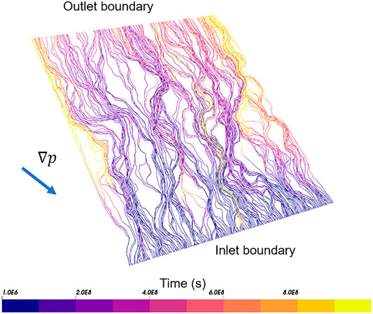
FIGURE 2. Pathlines from ConnectFlow transport simulation in plane-projected representation, colored by travel time. Direction of pressure gradient with respect to inlet and outlet boundaries is shown.

This results in distributions of τ (travel time) and β transport resistance over all particles, which are plotted in Figure 3. However, a comparison of results for the underlying DFN and plane-projected representations shows that a significant mismatch exists for both of these transport statistics in all stochastic realisations; the median value of each distribution is shifted by approximately half an order of magnitude for τ and a full order of magnitude for β, with the plane-projected results displaying shorter travel times and less transport resistance. The distributions are also narrower in the plane-projected case.

FIGURE 3

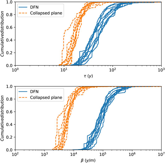
FIGURE 3. Cumulative distribution of τ and β of the trajectories of all DFN realizations.

These results indicate that the method of projection to a midplane described in section 2.3, while capturing some of the heterogeneity of the underlying DFN swarm, has not retained a full description of the transport properties of the simulated test BFZ. Particles transit through the BFZ too quickly, and thus corrections must be applied to the pathline results.

3.2. Downscaling Tests

The ability of the MARFA downscaling algorithm to reintroduce lost heterogeneity in the plane-projected BFZ representation and hence resolve the observed mismatches with τ and β in the DFN representation is investigated.

In figure 4 the cumulative distribution of the distance of all DFN realizations’ segments to the main BFZ plane can be seen. The cumulative distribution has been weighted by length, so that is independent of how the trajectories are discretized in segments. The vertical line shows the value of sigma distance σ. It can be seen that most of the length of the trajectories is found between the BFZ plane and a distance s. For that reason, the core sampling cubes are the ones used for the downscaling algorithm.

FIGURE 4

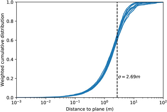
FIGURE 4. Cumulative distribution of the distance to plane of the DFN realizations' segments, weighted by length. The vertical black line shows the sigma distance.

As described in section 3.1, transport pathways are traced using ConnectFlow by means of particle tracking calculations with particles being placed uniformly over the inlet boundary. In all the calculations presented hereafter a correction is applied to account for flux-weighted particle injection. Moreover, the results of the ten realisations of the sampling cubes are merged into single sub-segment libraries. Details on the pre-processing procedures used are provided in Appendix 1: Processing Transport Pathways.

Two test cases are carried out. In the first test, denoted the Conservative case, a short pulse of a non-sorbing non-decaying radionuclide is injected at the BFZ boundary. Radionuclide transport is computed for each of the ten BFZ realizations using the related transport pathways and the rock matrix parameters listed in Table 1. The exercise is repeated first using the ten realisations of the collapsed plane without the downscaling algorithm and then by applying the downscaling algorithm on the same set of pathways. Moreover, the downscaling approach is also carried out using the single straight pathway representative of the homogeneous plane. The same procedure is used for the second test, denoted the Decay Chain case, where the 4n+2 chain of U238 is simulated. The decay chain is simplified as follows:

$\text{Cm}246\to \text{Pu}242\to \text{U}238\to \text{U}234\to \text{Th}230\to \text{Ra}226$

The radionuclide-specific parameters are listed in Table 2, whereas the parameters of the rock matrix are the same as in the Conservative case (Table 1). The source functions (Figure 5) are randomly selected from the 6,234 functions used to describe a hypothetical release at canister location in the so-called Forsmark Growing Pinhole Scenario (FGPS) (Selroos and Painter, 2012; Trinchero et al., 2020). FGPS was one of the modeling cases used in SR-Site, the safety assessment study for the planned repository for spent nuclear fuel at Forsmark, Sweden.

TABLE 1

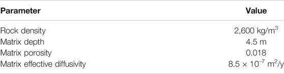
TABLE 1. Parameters of the rock matrix used in the Conservative case and the Decay Chain case.

TABLE 2

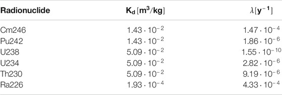
TABLE 2. Radionuclide-specific parameters for the Decay Chain case.

FIGURE 5

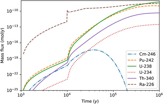
FIGURE 5. Plot of the source function of all radionuclides used in the Decay Chain case.

In both tests the downscaling simulations are carried out using the standard algorithm (SDA). In the calculations based on the homogeneous plane the projected sub-segment algorithm (PSSA) is also tested. It is worthwhile noting that in this latter set of calculations (i.e. straight pathway representative of a homogeneous BFZ), the local hydraulic gradient along the straight pathway is equal to the global gradient applied in the BFZ model (${\mathit{ϵ}}^i=3.06\cdot {10}^{-3}\text{cos}{30}^{\circ }$).

3.2.1. Conservative Case

The breakthrough curves computed for each BFZ realization (i.e. BFZ modeled as an explicit DFN) are first compared with the results obtained using transport pathways derived from the collapsed plane model and without downscaling. This comparison (Figure 6) shows that the collapsed plane model significantly under-estimates the radionuclide retention capacity of the BFZ system. This evidence is consistent with the statistical analysis (figure 3) which points out that transport pathways computed using the collapsed plane model are characterized by lower groundwater travel time and transport resistance. The low groundwater travel times affect the leading edge of the breakthrough curves and partly explain the observed higher peak values. The low values of transport resistance have an impact on mass exchange processes and thus mostly affect the late time part of the breakthrough curves, which explains the observed low level of the tail. When the downscaling option is used, the agreement with the DFN-based solutions is very good (Figure 6), which points out that the downscaling algorithm can properly reconstruct the variability lost during the DFN representation onto the plane. Moreover, this good agreement obtained using the standard downscaling algorithm (SDA) indicates that the collapsed plane heterogeneity is properly capturing the original geometrical tortuosity of the transport pathways. These conclusions, which are based on visual inspections of the breakthrough curves, are confirmed by the results of the Kolmogorov–Smirnov (K-S) test (Table 3) that gives significantly lower statistical values when the downscaling algorithm is applied.

FIGURE 6

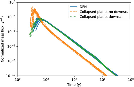
FIGURE 6. Conservative case: breakthrough curves of a non-sorbing non-decaying radionuclide computed using transport pathways obtained using the different realisations of the DFN model (blue continuous curves) compared with related calculations carried out using transport pathways derived from the collapsed plane model and without downscaling (orange dashed lines) and with related calculations where downscaling is applied (green dotted line).

TABLE 3

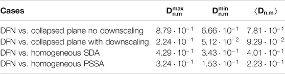
TABLE 3. Results of the Kolmogorov–Smirnov (KS) test for the different variant simulations of the Conservative case. The KS test is run for each DFN realization and related collapsed plane or homogeneous model and the results are provided in terms of maximum $\left(D_{n,m}^{max}\right)$, minimum $\left(D_{n,m}^{min}\right)$ and average $\left(\langle D_{n,m}\rangle \right)$ test statistic.

The comparison exercise is repeated using the single straight trajectory representative of the homogeneous plane. When the downscaling is performed using the SDA, the downscaled solution is characterized by an earlier breakthrough and a higher peak (Figure 7). This poor agreement is due to the tortuosity lost in the homogeneous representation. However, when the projected sub-segment algorithm (PSSA) is used, tortuosity is reconstructed by the downscaling algorithm and the agreement is significantly improved (Figure 7). The superior performance of the PSSA is also confirmed by the results of the KS test (Table 3).

FIGURE 7

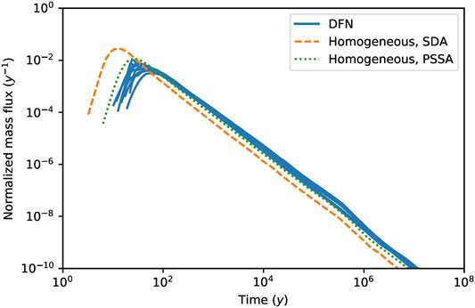
FIGURE 7. Conservative case: breakthrough curves of a non-sorbing non-decaying radionuclide computed using transport pathways obtained using the different realisations of the DFN model (blue continuous curves) compared with the calculation carried out using the single straight transport pathways derived from the homogeneous plane model and with downscaling applied using the standard algorithm (SDA) (orange dashed line) and with downscaling applied using the projected sub-segment algorithm (PSSA) (green dotted line).

3.2.2. Decay Chain Case

The results of the Decay Chain case are discussed here in terms of breakthrough curves of the daughter radionuclide Ra226. The results of the parent radionuclides are not shown for the sake of brevity.

When downscaling is not applied (Figure 8) and trajectories and related values of τ and β are taken from the collapsed planes, significantly larger mass fluxes are seen at the outlet boundary. These higher mass fluxes are related to the lower retention capacity of the BFZ system as represented with the collapsed plane model (Figure 3). Similar findings were already observed in the Conservative case.

FIGURE 8

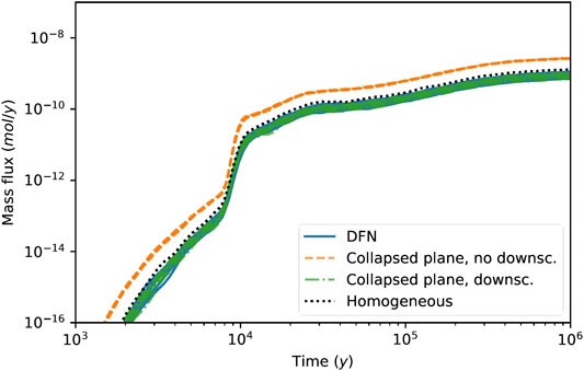
FIGURE 8. Decay Chain case: breakthrough curves of Ra226 computed using transport pathways obtained using the different realisations of the DFN model (blue continuous curves) compared with related calculations carried out using transport pathways derived from the collapsed plane model and without downscaling (orange dashed lines), with related calculations carried out using transport pathways derived from the collapsed plane model and with downscaling applied using the standard algorithm (SDA) (green dashed-dotted lines) and with calculations carried out using the single straight transport pathways derived from the homogeneous plane model and with downscaling applied using the projected sub-segment algorithm (PSSA) (orange dotted line).

When downscaling is applied, using the different sets of trajectories computed from the different realisations of the collapsed plane model and SDA, the observed Ra226 breakthrough curves agree well with the corresponding solutions computed using the explicit DFN representation of the BFZ (Figure 8). A good agreement is also observed when using the PSSA and the single straight trajectory representative of the homogeneous plane (see same figure).

Due to the presence of decay, a good indicator for the goodness of fit between the different models is the relative error in recovered mass. For a collapsed plane or single straight trajectory model n compared to a DFN model m, the relative error ${\epsilon }_{n,m}$ is defined as:

${\epsilon }_{n,m}=\frac{M_n-M_m}{M_m}(9)$

where $M_n$ and $M_m$ are the values of recovered mass for models n and m.

The results for the recovered mass test are shown in Table 4. Lower relative errors are observed in the collapsed plane model when the downscaling algorithm is applied. The good agreement between the single straight trajectory with PSSA and the DFN model is also confirmed by the test results.

TABLE 4

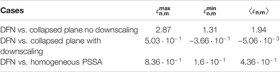
TABLE 4. Results of the mass test for the different variant simulations of the Decay Chain case. The test is run for each DFN realization and related collapsed plane or homogeneous model and the results are provided in terms of maximum $\left({\epsilon }_{n,m}^{max}\right)$, minimum $\left({\epsilon }_{n,m}^{min}\right)$ and average $\left(\langle {\epsilon }_{n,m}\rangle \right)$ test statistic.

4. Discussion

As expected, the model obtained by projecting the flow and transport properties of a 3D fracture swarm onto a plane does not fully replicate the particle transport behavior of the full DFN. By removing heterogeneity normal to the midplane and restricting pathlines to a 2D surface, retention within the system is underestimated and particle travel times and transport resistance are systematically shorter.

A correction method, based on a previously published downscaling algorithm (Painter and Cvetkovic, 2005), has been tested using two test cases focused on the transport of specific radionuclides. The algorithm operates by statistically sampling libraries of triplets $\left|{\text{Δ}}_i,{\tau }_i,{\beta }_i\right|$, which are in turn built using simplified but statistically representative DFN models (referred to as sampling cubes). Correlation in high/low velocity zones is accounted for by using a Markov chain. When the downscaling algorithm is used, the geometric information of the collapsed-plane-based transport pathways is used whereas the particles are advanced according to the sampled triplet values. An additional set of calculations has been carried out where the downscaling algorithm has been applied to a single straight trajectory representative of a homogeneous plane.

When applied to the heterogeneous collapsed plane, the downscaling approach is shown to accurately reconstruct the lost transport heterogeneity and the resulting radionuclide breakthrough curves agree well with the DFN-based solution. However, when the single straight trajectory is used, the resulting breakthrough curves show early arrivals and, in the case of the decaying radionuclide Ra-226, higher mass flux. This mismatch is caused by the lost tortuosity of the homogeneous model. Hence, an alternative implementation of the downscaling algorithm has been proposed, in which trajectory segments are projected along the principle direction. The modified algorithm is shown to provide very good results when applied to transport pathways derived from homogeneous models.

The generality of the Markov model applied here means that it is in principle applicable to a DFN based on any kind of empirical relationship and thus not only limited to the set of parameters and correlations described in Section 2.2. As the method is based on libraries which are constructed using an identical recipe to the DFN model, this consistency is ensured. The central assumption of the Markov method here is that the triplet $\left|\text{Δ},\tau ,\beta \right|$ for each pathline segment depends only on the preceding segment. This method may therefore be less appropriate for DFN models in which some longer-range persistence along a pathline is present that cannot be captured by the Markov approximation (Painter and Cvetkovic, 2005).

The simple case presented in this article consists of a single synthetic BFZ fracture swarm with a single set of DFN parameter values; only one library of pathline legs is therefore required for the MARFA downscaling method to be applied. More than one library must be generated in order to apply the method to the realistic site-scale case, in which multiple BFZ are present, with DFN parameter values varying between BFZ and in some cases between distinct layers or regions within a single BFZ. The increased computational overhead of multiple library generation can be mitigated by grouping similar BFZ into classes based on their orientation and fracture intensity, with the pathline legs within each class described by a single library. This approach is now being tested in a subsequent phase of this study.

The computational speedup provided by the use of the collapsed plane model in comparison to the full DFN model is illustrated by the runtime provided in Tables 5, 6. For the Conservative case, the time taken by ConnectFlow to solve for flow and generate pathlines is reduced by more than two orders of magnitude. Although there is an increase in the MARFA radionuclide tracking runtime due to the application of the downscaling algorithm, this is small in comparison and so a mean speedup of 20x is achieved across the 10 realisations. For the Conservative case, the ConnectFlow calculation is identical but the MARFA runtime accounts for a greater proportion of the total runtime due to the additional expense of modeling a decay chain, reducing the mean speedup to 3x. It should be noted that, for this simple synthetic model, the relative cost of constructing a library of pathline segments is high in comparison to the time taken to perform radionuclide tracking calculations in the full DFN model, with a mean ConnectFlow runtime for one realization of the sampling cube DFN model approximately 3 times greater than the runtime for the full DFN model. This is a result of the relative sizes of the models (homogeneous DFN in a 100 × 100 × 100 m domain for the sampling cube, as compared to a narrow fracture swarm in a 500 × 500 × 500 m domain for the full DFN model), and therefore not representative of the relative cost of constructing the library when scaled to the realistic case in which the full DFN model is much larger and more complex relative to the sampling cube. Further to this point, a pathline library must only be constructed once for each class of BFZ in the model (as defined in the previous paragraph), whereas real-world applications such as safety assessments of geological repositories of spent nuclear fuel typically necessitate multiple iterations of particle tracking calculations with varying boundary conditions. In such a case, the cost of library construction is thus expected to be much smaller relative to the total computation time saved by the use of the collapsed plane model.

TABLE 5

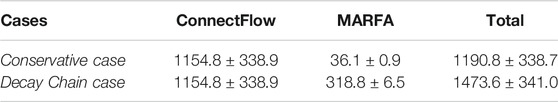
TABLE 5. DFN model runtime in seconds for the Conservative case and Decay Chain case, calculated as a mean over 10 realisations $\pm 1\sigma$ and separated into ConnectFlow and MARFA components.

TABLE 6

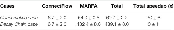
TABLE 6. Collapsed plane runtime in seconds for the Conservative case and Decay Chain case, calculated as a mean over 10 realisations $\pm 1\sigma$ and separated into ConnectFlow and MARFA components. Approximate speedup over the DFN model runtime in Table 5 is also provided.

5. Summary and Conclusion

A method for the simplification of complex DFN models of BFZ damage zones has been tested. The method consists of first upscaling the DFN to an ECPM model, using a flux-based methodology. The resulting ECPM model is then projected onto the mid-plane of the BFZ. The plane-projected model is much more computationally tractable and provides an accurate description of global groundwater flow patterns. However, during the upscaling, local heterogeneity in flow and transport properties and related local choking effects are lost and thus related transport calculations are biased toward smaller values of groundwater travel time and transport resistance.

We have shown that the lost transport heterogeneity can be reconstructed by combining the plane-projected models with libraries of the two transport controlling parameters: the groundwater travel time and the transport resistance. These libraries are pre-computed using small DFN models (sampling cubes) with fracture statistics equal to those at the core of the BFZ model. The reconstruction of the groundwater velocity field and the transport resistance is carried out by assuming that the Lagrangian velocity follows a Markov process; i.e. the velocity in a fracture segment depends only on the velocity of the preceding segment. This sampling methodology was originally developed to extrapolate velocity distributions from small-to much larger-scale DFN models. To adapt the methodology to the foreseen application, a modification has been introduced, which consists of projecting fracture segments of the sampling cubes along principal directions. This modification is needed to account for the tortuosity of transport pathways of DFN models, which is lost in homogeneous representations of the BFZ. When the BFZ is represented as a heterogeneous collapsed plane this modification is not needed and the original algorithm provides good agreement with the synthetic solution.

The proposed downscaling approach is shown to provide a very accurate description of radionuclide breakthrough curves at compliance or outlet boundaries. The promising results shown in this work are of interest for a broad number of applications related to contaminant transport in fractured rocks. These include safety assessment calculations for spent nuclear fuel repositories, studies for the remediation of polluted sites or, in the context of nuclear nonproliferation, the detection of chemical signatures following underground explosions.

Data Availability Statement

The raw data supporting the conclusions of this article will be made available by the authors, without undue reservation.

Author Contributions

ConnectFlow simulations were carried out by TW and GG, and MARFA simulations by JS and PT. All authors contributed to the design of the study, interpretation of numerical experiments, and preparation of the manuscript.

Funding

This work was funded by Svensk Kärnbränslehantering AB (SKB).

Licenses and Permissions

This manuscript has been co-authored by UT-Battelle, LLC under Contract No. DE-AC05-00OR22725 with the U.S. Department of Energy. The United States Government retains and the publisher, by accepting the article for publication, acknowledges that the United States Government retains a non-exclusive, paidup, irrevocable, world-wide license to publish, or reproduce the published form of this manuscript, or allow others to do so, for United States Government purposes. The Department of Energy will provide public access to these results of federally sponsored research in accordance with the DOE Public Access Plan (http://energy.gov/downloads/doe-public-access-plan).

Conflict of Interest

TW and GG were employed by Jacobs United Kingdom Ltd. JS and PT were employed by AMPHOS 21 Consulting S.L. J-OS was employed by Svensk Kärnbränslehantering AB (SKB).

The remaining author declares that the research was conducted in the absence of any commercial or financial relationships that could be construed as a potential conflict of interest.

Appendix

Processing Transport Pathways

The set of transport pathways, computed by ConnectFlow assuming uniform particle injection, is re-sampled to mimic a flux-weighted injection. The re-sampling algorithm is as follows (algorithm 1):

(1) Calculate water flux at the inlet of each transport pathway, $q_i$ [L³T⁻¹].

(2) Sort the set of pathways in order of increasing flux at the inlet and construct the cumulative distribution (CD) function by assigning a probability of $q_i/Q_{tot}$ to the ith pathway, where $Q_T={{{\displaystyle \sum }}^{\text{}}}_{i=1}^N{q}_i$ and N is the total number of transport pathways.

(3) Randomly sample the CD and store the selected transport pathway in memory.

(4) Repeat step 3 M times and write the new set of transport pathway in an ASCII file.

In the calculations of section 3$M=1000$ whereas N depends on the realization and varies between 820 and 1,652 while for the collapsed planes around 300 pathways are used. A sensitivity analysis to M has been carried out to ensure that statistical ergodicity is attained. It is worthwhile noting that the methodology above implies that some of the original transport pathways are sampled multiple times whereas other pathways, with low flux at the inlet, are never sampled.

The libraries used for the downscaling algorithm are obtained from ten equi-probable sampling cubes. The related set of particle trajectories (one set for each realization and each principal direction) are merged into a single library for each principal direction using the following methodology:

(1) Calculate the inlet flux for every transport pathway and for all the 10 sampling cubes.

(2) Construct a CD function for each sampling cube as in step 2 of algorithm 1.

(3) Randomly select a sampling cube assuming a uniform distribution.

(4) Select a transport pathway from the chosen sampling cube as in step 3 of algorithm 1.

(5) Repeat steps 1–3 M times until enough trajectories are sampled and write the library file.

(6) The original set of transport pathways of each sampling cube consists of 1,000 particle trajectories and the library file is built by setting $M=10000$.

References

Aaltonen, I., Kosunen, P., Mattila, J., Engström, J., Paananen, M., Paulamäki, S., et al. (2016). Tech. Rep. POSIVA Report 2016-16. Geology of Olkiluoto. Eurajoki, Finland: Posiva Oy.

CrossRef Full Text | Google Scholar

Baxter, S., Hartley, L., Hoek, J., Myers, S., Tsitsopoulos, V., and Williams, T. (2019). Tech. Rep. SKB Report R-19-01. Upscaling of brittle deformation zone flow and transport properties. Stockholm, Sweden: Svensk Kärnbränslehantering AB (SKB).

CrossRef Full Text | Google Scholar

Bear, J. (1972). Dynamics of fluids in porous media. New York, NY: American Elsevier.

CrossRef Full Text | Google Scholar

Benke, R., and Painter, S. (2003). Modeling conservative tracer transport in fracture networks with a hybrid approach based on the Boltzmann transport equation. Water Resour. Res. 39. doi:10.1029/2003WR001966

CrossRef Full Text | Google Scholar

Bolster, D., Barahona, M., Dentz, M., Fernandez-Garcia, D., Sanchez-Vila, X., Trinchero, P., et al. (2009). Probabilistic risk analysis of groundwater remediation strategies. Water Resour. Res. 45. doi:10.1029/2008WR007551

CrossRef Full Text | Google Scholar

Cacas, M. C., Ledoux, E., de Marsily, G., Tillie, B., Barbreau, A., Durand, E., et al. (1990). Modeling fracture flow with a stochastic discrete fracture network: calibration and validation: 1. the flow model. Water Resour. Res. 26, 479–489. doi:10.1029/WR026i003p00479

CrossRef Full Text | Google Scholar

Comolli, A., Hakoun, V., and Dentz, M. (2019). Mechanisms, upscaling, and prediction of anomalous dispersion in heterogeneous porous media. Water Resour. Res. 55, 8197–8222. doi:10.1029/2019WR024919

CrossRef Full Text | Google Scholar

Gelhar, L. W., and Axness, C. L. (1983). 3-dimensional stochastic-analysis of macrodispersion in aquifers. Water Resour. Res. 19, 161–180. doi:10.1029/WR019i001p00161

CrossRef Full Text | Google Scholar

Hakoun, V., Comolli, A., and Dentz, M. (2019). Upscaling and prediction of Lagrangian velocity dynamics in heterogeneous porous media. Water Resour. Res. 55, 3976–3996. doi:10.1029/2018WR023810

CrossRef Full Text | Google Scholar

Hartley, L., Appleyard, P., Baxter, S., Hoek, J., Joyce, S., Mosley, K., et al. (2018). Tech. Rep. POSIVA working Report 2017-32. Discrete fracture network modelling (Version 3) in support of Olkiluoto site description 2018. Eurajoki, Finland: Posiva Oy.

CrossRef Full Text | Google Scholar

Hyman, J. D., Dentz, M., Hagberg, A., and Kang, P. K. (2019). Emergence of stable laws for first passage times in three-dimensional random fracture networks. Phys. Rev. Lett. 123, 248501. doi:10.1103/PhysRevLett.123.248501

PubMed Abstract | CrossRef Full Text | Google Scholar

Jackson, C., Hoch, A., and Todman, S. (2000). Self-consistency of a heterogeneous continuum porous medium representation of a fractured medium. Water Resour. Res. 36, 189–202. doi:10.1029/1999WR900249

CrossRef Full Text | Google Scholar

Jacobs, (2018). Tech. Rep. Jacobs report Jacobs/ENV/CONNECTFLOW/15. ConnectFlow technical summary release 12.0.

CrossRef Full Text | Google Scholar

Joyce, S., Simpson, T., Hartley, L., Applegate, D., and Hoek, J. (2010). Tech. Rep. R-09-20. Groundwater flow modelling of periods with temperate climate conditions: Forsmark. Stockholm, Sweden: Svensk Kärnbränslehantering AB (SKB).

CrossRef Full Text | Google Scholar

Karra, S., Makedonska, N., Viswanathan, H. S., Painter, S. L., and Hyman, J. D. (2015). Effect of advective flow in fractures and matrix diffusion on natural gas production. Water Resour. Res. 51, 8646–8657. doi:10.1002/2014WR016829

CrossRef Full Text | Google Scholar

Kwicklis, E., Lu, Z., Middleton, R., Miller, T., Bourret, S., and Birdsell, K. (2019). Numerical evaluation of unsaturated-zone flow and transport pathways at Rainier Mesa, Nevada. Vadose Zone J. 18, 190005. doi:10.2136/vzj2019.01.0005

CrossRef Full Text | Google Scholar

Makedonska, N., Hyman, J. D., Karra, S., Painter, S. L., Gable, C. W., and Viswanathan, H. S. (2016). Evaluating the effect of internal aperture variability on transport in kilometer scale discrete fracture networks. Adv. Water Resour. 94, 486–497. doi:10.1016/j.advwatres.2016.06.010

CrossRef Full Text | Google Scholar

Neretnieks, I. (1980). Diffusion in the rock matrix: an important factor in radionuclide retardation. J. Geophys. Res. 85, 4379–4397. doi:10.1029/JB085iB08p04379

CrossRef Full Text | Google Scholar

Painter, S., Cvetkovic, V., Mancillas, J., and Pensado, O. (2008). Time domain particle tracking methods for simulating transport with retention and first-order transformation. Water Resour. Res. 44 (1), W01406. doi:10.1029/2007WR005944

CrossRef Full Text | Google Scholar

Painter, S., and Cvetkovic, V. (2005). Upscaling discrete fracture network simulations: an alternative to continuum transport models. Water Resour. Res. 41. doi:10.1029/2004WR003682

CrossRef Full Text | Google Scholar

Painter, S., and Mancillas, J. (2013). Tech. Rep. POSIVA working Report 2013-01. MARFA user’s manual: migration analysis of radionuclides in the far field. Eurajoki, Finland: Posiva Oy.

CrossRef Full Text | Google Scholar

Posiva, (2013). Tech. Rep. POSIVA Report 2011-02. Olkiluoto site description 2011. Eurajoki, Finland: Posiva Oy.

CrossRef Full Text | Google Scholar

Poteri, A., Nordman, H., Pulkkanen, V.-M., and Smith, P. (2014). Tech. Rep. Working Report 2017-23. Radionuclide transport in the repository near-field and far-field. Eurajoki, Finland: Posiva Oy.

CrossRef Full Text | Google Scholar

Sanchez-Vila, X., Guadagnini, A., and Carrera, J. (2006). Representative hydraulic conductivities in saturated groundwater flow. Rev. Geophys. 44, RG3002. doi:10.1029/2005RG000169

CrossRef Full Text | Google Scholar

Selroos, J.-O., and Painter, S. L. (2012). Effect of transport-pathway simplifications on projected releases of radionuclides from a nuclear waste repository (Sweden). Hydrogeol. J. 20, 1467–1481. doi:10.1007/s10040-012-0888-5

CrossRef Full Text | Google Scholar

SKB (2010). Radionuclide transport report for the safety assessment SR-Site. Tech. Rep. TR-10–50, Stockholm, Sweden: Svensk Kärnbränslehantering AB (SKB).

CrossRef Full Text | Google Scholar

Trinchero, P., Painter, S., Ebrahimi, H., Koskinen, L., Molinero, J., and Selroos, J.-O. (2016). Modelling radionuclide transport in fractured media with a dynamic update of Kd values. Comput. Geosci. 86, 55–63. doi:10.1016/j.cageo.2015.10.005

CrossRef Full Text | Google Scholar

Trinchero, P., Painter, S. L., Poteri, A., Sanglas, J., Cvetkovic, V., and Selroos, J.-O. (2020). A particle-based conditional sampling scheme for the simulation of transport in fractured rock with diffusion into stagnant water and rock matrix. Water Resour. Res. 56, e2019WR026958. doi:10.1029/2019WR026958. E2019WR026958

CrossRef Full Text | Google Scholar

Trinchero, P., Sánchez-Vila, X., and Fernàndez-Garcia, D. (2008). Point-to-point connectivity, an abstract concept or a key issue for risk assessment studies? Adv. Water Resour. 31, 1742–1753. doi:10.1016/j.advwatres.2008.09.001

CrossRef Full Text | Google Scholar