Quantifying Short-Term Erosion and Deposition in an Active Gully Using Terrestrial Laser Scanning: A Case Study From West Tennessee, USA

Introduction

Gullies are linear channels on hillslopes with steep sided and low width-depth ratio that expand through repeated flash flooding (Bocco, 1991; Morgan, 1996; Knighton, 1998). Gullies can be classified as ephemeral and permanent (Bull and Kirkby, 1997; Poesen et al., 1998; Poesen et al., 2003; Poesen et al., 2006). Ephemeral gullies are routinely infilled, leaving behind depressions that may promote the development of new gullies, while permanent gullies experience more pronounced erosion than deposition and are easily identifiable in the field (Bull and Kirkby, 1997). Some gullies may begin as micro-relief rills that are usually <0.3 m in depth and <0.3 m in width (Nearing et al., 1997; Knighton, 1998; Gao, 2013). Depressions left behind by landslides can be further incised to gullies by subsequent storms (Vittorini, 1972). Gullies can also be formed by piping or tunnel erosion (Downes, 1946), especially in areas with upper loamy and lower high clay-content layers where subsurface flow along the low-permeability, high clay-content layer may induce the collapse of the upper soil layer, initiating gully depression (Zhu, 2003). A common criterion to define gullies is based on a minimum width of 0.3-m and depths from 0.5 to 30-m with a threshold minimum cross-sectional area of 929 cm² (1 ft²), named as the “square foot criterion” (Hudson, 1981; Poeson, 1993).

Gully formation has been mainly attributed to human influences, although they can be formed naturally (Trimble, 1974; Trimble, 1985; Bocco, 1991). Changes in land use, such as the conversion of forest to farmland, disrupt the natural landscape equilibrium and alter the diversion and concentration of surface flows (Hudson, 1981). Agricultural practices are the most common drivers of human-induced gully formation, the effects of which are observed everywhere from the rainforest-turned-farmland areas in Brazil to the deserts in the southwestern United States (Trimble, 1974; Trimble, 1985; Morgan, 1996).

Despite the significance of gully erosion on hillslope stability and agriculture productivity, few studies have investigated the short-term sediment dynamics within the gully, partially due to the lack of reliable methods to quantify changes in microtopography. Early studies on gully erosion were primarily based on field measurements that are time consuming and labor intensive (Ireland et al., 1939; Leopold and Miller, 1956; Betts et al., 2003). Current advances in Light Detection and Ranging (LiDAR) technology provide an opportunity to quantify gully erosion by producing high-resolution digital elevation models (DEMs). LiDAR data has been commonly collected using airborne and terrestrial laser scanning sensors (Heritage and Hetherington, 2007). The airborne laser scanning (ALS) is suited for surveying large areas at regional spatial scales, producing DEMs with horizontal resolutions ranging from 0.5- to 3-m (Lohani and Mason, 2001; Challis, 2006; Cavalli et al., 2008). Terrestrial laser scanning (TLS) is usually used for local-scale survey, producing DEMs of much higher vertical (mm) and horizontal resolutions (mm to cm levels; Hohenthal et al., 2011). Both ALS and TLS have been used to quantify topographic changes. For example, Perroy et al. (2010) used ALS and TLS to quantify gully erosion on Santa Cruz Island, California and found that these estimates were comparable to those from the existing field survey based on total stations. ALS and TLS studies of sea-cliff changes in Del Mar, California suggested that estimates of cliff retreat volumes are highly correlated using both methods, but TLS captures small changes in topography more consistently than ALS (Young et al., 2010). In general, TLS is a more suitable technology for capturing microtopographic changes due to its high vertical and horizontal resolutions (Milan et al., 2007; Kukko et al., 2008; Corsini et al., 2013; Croke et al., 2013; Picco et al., 2013; Bangen et al., 2014; Lu et al., 2019).

Many studies have investigated the effect of DEM resolution on the measurement of topographic indices (e.g., Wolock and Price, 1994; Zhang and Montgomery, 1994; Thompson et al., 2001; Woolard and Colby, 2002; Deng et al., 2007; Yang et al., 2014; Charrier and Li, 2012; Li, 2015; Lu et al., 2017). Although the general assumption is that the measurement on higher-resolution DEMs is more precise than those on lower-resolution DEMs, the impact of DEM resolution varies for different topographic indexes. For example, Zhang and Montgomery (1994) examined the changes in slope and watershed boundaries for DEMs of 2-, 4-, 10-, 30-, and 90-m resolutions and concluded that the 10-m DEM is a compromise between precision and efficiency for the topographic analysis at landscape scales. Charrier and Li (2012) assessed the DEM resolution effect on stream network and watershed delineation and concluded that while higher resolution DEM, such as 1-m, is better for stream network delineation, such high-resolution DEM may complicate watershed boundary delineation due to the influence of minor topographic features. They suggested using a relatively low-resolution DEM, such as 5- or 10-m, to delineate the watershed boundary (Charrier and Li, 2012).

Recent studies have also investigated the effect of DEM resolution (or point spacing) on estimated erosion and deposition volumes using TLS. Lu et al. (2017) investigated the effect of grid size on hillslope erosion and deposition based on TLS-derived DEMs and found that both the areas and volumes of detectable erosion and deposition decrease as the resolution coarsens although the changes in erosion are apparently less sensitive than the changes in deposition. However, these findings were concluded from the measurement of detectable erosion and deposition on a rill dominated hillslope, while few studies have investigated the effect of DEM resolution on gully erosion and deposition (Dai et al., 2019).

The purpose of this study is to quantify sediment redistribution using TLS in an active gully within a United States state park in west Tennessee that has been affected by historical and contemporary land management. We also seek to examine how the spatial resolution of TLS-derived DEMs affect the estimates of sediment volume. The objectives of this study are to: 1) examine the pattern of erosion and deposition and estimate their areal and volumetric changes based on the difference between two high resolution DEMs of the gully that were surveyed using TLS on December 24, 2014 and February 8, 2015; and 2) explore the relationship between changing spatial resolution of the TLS-derived DEMs and the resulting estimates of erosional and depositional sediment volumes. This study will improve the understanding of sediment erosional and depositional processes within the gully and provide useful guidance for other TLS studies on gully sediment dynamics.

Study Area

Our study area is the 54.5 km² Meeman-Shelby Forest State Park that is located in the humid sub-tropical climate regime (Cfa), according to the Köppen climate classification, along the eastern bluff of the Mississippi River within Shelby County, Tennessee, southeastern United States (Figures 1A,B). The mean annual precipitation is 1,360 mm, occurring mostly in the spring and early winter (U.S. Climate Data, 2016, Figure 1A). Temperature peaks in July with a mean high of 33°C and low of 23°C, respectively, while January is the coldest month with a mean high of 9.9°C and low of 0.3°C, respectively (U.S. Climate Data, 2016, Figure 1A).

FIGURE 1

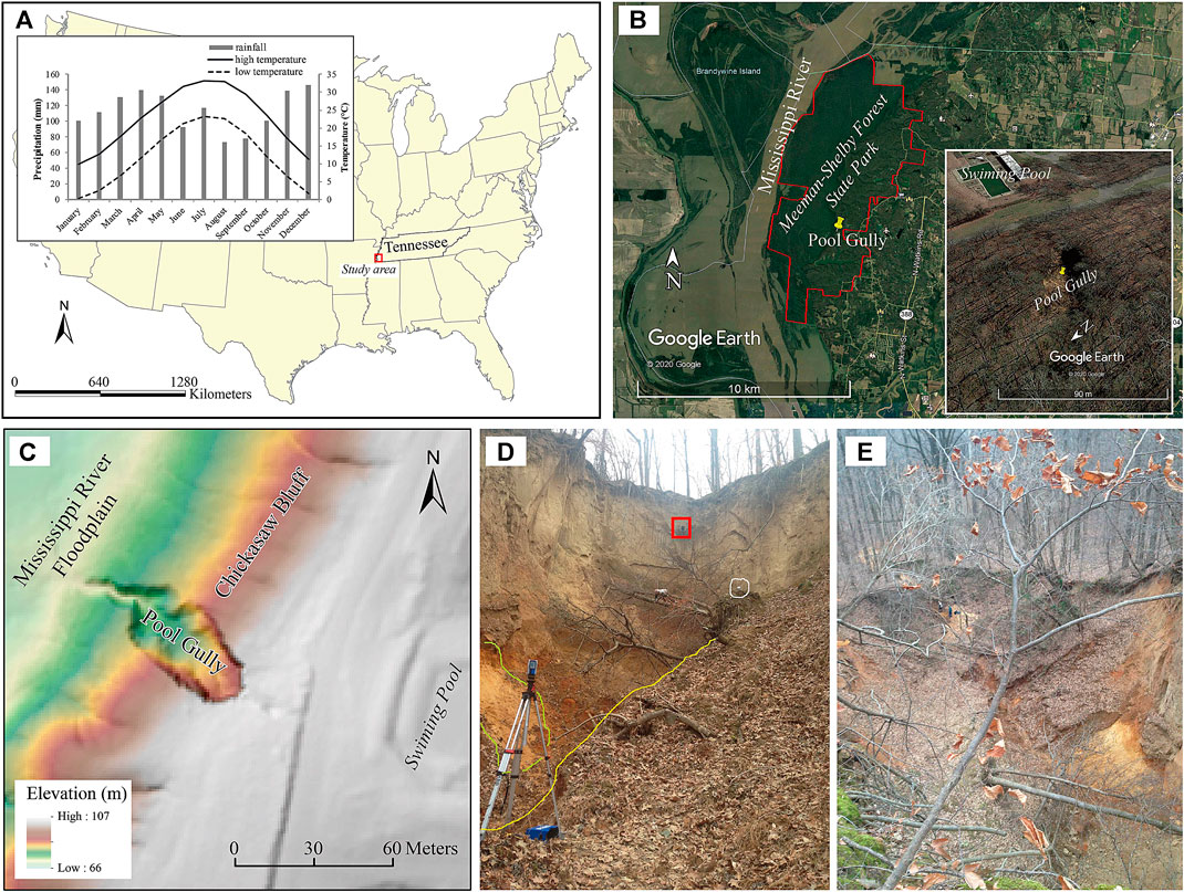
FIGURE 1. (A, B) The study site within the Meeman-Shelby Forest State Park in west Tennessee. The inset graph in (A) shows monthly average high and low temperature and precipitation (1981–2010) for Shelby County, Tennessee (U.S. Climate Data, 2016). The Google Earth screen shots in (B) are based on the high-resolution images updated in 2020. The red polygon represents the park boundary. The pool gully is close to the swimming pool and is clearly identifiable on the image. (C) Shaded-relief 1-m DEM showing the Mississippi River floodplain and the Chickasaw Bluff with the marked pool gully and the swimming pool in the park. The DEM is generated using the ALS point cloud (0.5 m spacing) surveyed by the USGS in 2012. (D) A field photo facing the gully head. The discharge pipe from the swimming pool is visible in the red box at the top of the photo. The TLS and its tripod are at the left-bottom of the photo. The white box marks a sphere target for the TLS scan. The yellow line marked the bottom of the gully and a fresh collapsed slope on the left side of the gully. (E) another field photo facing downslope of the gully. Falling trees and fresh collapsed slopes from these two field photos indicate very active erosion-deposition processes in this gully.

This area belongs to the Mississippi embayment of the Coastal Plain physiographic province. The western half of the park is on the floodplain of the Mississippi River and the eastern half on the Mississippi river terrace, known locally as the Chickasaw Bluff because it rises abruptly from the floodplain (Barnhardt, 1988a). Most sand and gravel terrace deposits on the Chickasaw Bluff are covered by a sequence of surficial loess units from the mid to late Pleistocene (Rodbell et al., 1997). The terrace deposits were developed on top of the sand, silt, clay, and lignite of the Eocene Cockfield Formation and the Plio-Pleistocene Upland Complex. The dominant soil type of this area, Memphis silt loam, is developed in the surficial loess units with a varied thickness of 5–25 cm (Sease et al., 1970).

The western floodplain part of the park is covered by hardwood forest, including bald cypress and swamp tupelo (Tennessee State Parks, 2016). The terrace part is covered by oak, beech, hickory, and sweet gum forest, providing habitat for hundreds of birds, deer, and small mammals, such as beaver and fox (Barnhardt, 1988a; Tennessee State Parks, 2016).

The surficial loess units on the bluff have been dissected by a set of gullies and valleys. In addition to the natural geomorphic processes, human activity has played an important role on soil erosion and gully formation in this area since the early Mississippian period (1000–1200 CE) (Dotterweich et al., 2014). An early sign of human-induced erosion was observed at the end of the first millennia CE and through the following several centuries, erosion in this area was likely accelerated due to Native Americans managed woodland fires and clear-cuts (Dotterweich et al., 2014). After this period, the uplands along the Chickasaw Bluff were likely abandoned during the 16th and 17th centuries due to the flooding, diseases, population movement, slave raids, and warfare that decimated the indigenous population, leading to a period of woodland regeneration, landscape revegetation, and geomorphic stability (James, 2011; Dotterweich et al., 2014).

A population boom in the middle 1800s initiated rapid deforestation to bolster a burgeoning hardwood industry in this area. The transition from forest to farmland was detrimental to landscape stability and exacerbated by unregulated farming practices (Barnhardt, 1988b; Barnhardt, 1989). At the peak of the transition, over 50% of the land within the park was actively farmed (Bennett, 1928). The federal government established a “recreational demonstration area” managed by the National Park Service in 1935. The project included major reclamation efforts. Hundreds of check dams were constructed within active gully channels and, in some cases, the channels were re-engineered entirely. Barnhardt (1989) examined the effectiveness of the extensive soil conservation program in the MSFSP and concluded that mitigation efforts were largely ineffective, as heavy rainfall events (the mean annual precipitation is 1,360 mm in this area) tended to re-invigorate gully activity, although certain areas appeared to have achieved a degree of stability.

Despite the significant impact of gully erosion on this area in recent history, previous studies focused primarily on the long-term average erosion (Barnhardt, 1988b; Barnhardt, 1989; Dotterweich et al., 2014), whereas few studies have investigated the short-term dynamics of gullies in the loess composed terraces along the Mississippi River (Barnhardt, 1988b). This study focuses on a “pool gully” at the out spout of the drainage system from a nearby swimming pool in the southern portion of the park (Figures 1B–E). The gully is actively carving into the river terrace and was formed after the pool and drainage system was installed (personal communication, Tennessee State Park Service). The United States Geological Survey (USGS) conducted an airborne LiDAR survey (ALS) of this area in January 2012 (data are available from http://nationalmap.gov/viewer.html). The gully is apparent on the shaded-relief 1-m DEM (Figure 1C) generated from this ALS’s point cloud (about 0.5 m spacing). Based on this DEM, this gully is approximately 28 m at its widest in 2012, with a headwall depth of approximately 18 m and a length of 70 m. The catchment area of the pool deck is approximately 4,070 m². The 45.7 cm diameter pipe (marked in Figure 1D) discharges drainage at flow rates ranging from 9.8 to 13.1 L per second from the pool deck including a biweekly flush of significant volumes of water for maintenance during the operational period from May to July. Park authorities and study of historical aerial photos indicate that the pool was constructed between 1969 and 1973 and has been continuously used since then.

Methods

Terrestrial Laser Scanning Data Acquisition and Registration

We conducted two TLS surveys on December 24, 2014 and February 8, 2015, respectively, to test the feasibility of using TLS to monitor short-term sediment dynamics in this gully. Since the ALS survey of this area was conducted by the USGS during the winter period (January 2012), we selected a similar period for our TLS surveys in a broader context of monitoring gully erosion using both ALS and TLS. The erosion and deposition during this period are likely driven by the precipitation and potential freeze-thaw processes because of the closure of the swimming pool during the winter months.

We used a 1,550-nm FARO Focus3D X 330 TLS (FARO, Inc.) for the surveys. This TLS has a 360° horizontal and 307° vertical scanning view, a laser spot size of 2.25-mm (0.19 mrad beam divergence). It can capture features within a radius of 330 m at a frequency of 976,000 points per second. The TLS was set with a range accuracy of ±2 cm at a range of 20-m and were operated with a consistent height of 1.65 m from the top of the scanner on a tripod to the ground. Each scan roughly takes 8 min to collect point cloud and digital photos. It captures about 24–33 million points (∼65% of points were intercepted) within the gully (Table 1).

TABLE 1

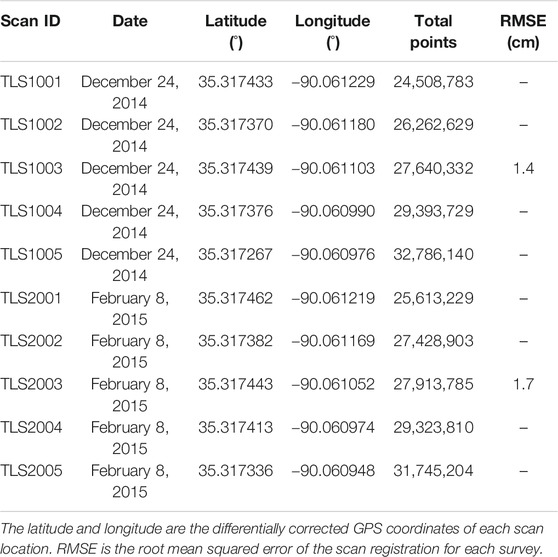
TABLE 1. The information for the five TLS scans collected in an active gully in Meeman-Shelby Forest State Park in Shebly County, Tennessee, on December 24, 2014 and February 8, 2015, respectively.

For a TLS survey of gully topography, multiple scans are needed from different locations to prevent possible occlusions of the laser points from an individual location by the rugged terrain within the gully. Carr et al. (2013) provided several recommendations to determine the TLS scan locations: 1) use a minimum of four control points within the view of each scan; 2) promote substantial overlap between different scans; and 3) conduct multiple perspective scans for the area of interest. Following these recommendations, we conducted five TLS scans within the gully for each survey. Four reference sphere targets (diameter of 139 mm) were evenly placed in the gully and used as control points to help the registration of the five scanned point clouds. A Trimble GeoXH global positioning system (GPS, Trimble, Inc.) was used to measure the locations of the four sphere targets and the location of each scan (Table 1). The GPS positions were differentially corrected using Trimble GPS Pathfinder Office (version 4.10) with an overall accuracy of ±15 cm.

Point cloud registration of the five scans at each survey was conducted using the Cloud-to-Cloud registration tool in FARO SCENE software (FARO, 2015) based on the matching of the sphere targets. The differentially corrected GPS coordinates of the sphere targets were used in the Cloud-to-Cloud registration tool to convert the coordinate system of the registered scan from a local Cartesian projection to the Universal Transverse Mercator (UTM) projection. We used the most centrally located scan (Scan #3) as the reference and the other four scans were registered to match this reference. The root mean squared error (RMSE) for the sphere targets was computed within the Cloud-to-Cloud registration tool. The RMSE of the registration was 1.4 and 1.7 cm for the surveys on December 24, 2014 and February 8, 2015, respectively (Table 1).

The point clouds of the two surveys were not aligned properly because of the relatively large uncertainties of the GPS coordinates that were used to define the coordinate system of the point clouds. We used an open source software, CloudCompare (https://danielgm.net/cc/), to improve the registration of these two point clouds. We manually picked a set of tie points from each point cloud that represent fixed objects in the area, such as utility poles, the outlet of the discharge pipe, and the intersections of major branches and trunks of stable trees. We tried out different tie points to reduce the registration error. Specifically, the tie points with registration errors of >2.5 cm were removed, and new tie points were tested to improve the registration accuracy. We reached a RMSE of 1.5 cm based on the selection of five tie points.

Digital Elevation Model Generation

For each survey, ground surface points were separated from the points that represent vegetation or other noises to generate ground surface DEMs using Quick Terrain Modeler (QTM) (Applied Imagery, 2009). Removing vegetation and noise points is an iterative process depending on the topographical complexity (Hofle et al., 2013). For this study, the near-vertical slope of the gully sidewalls and headwall hampered the removal of vegetation. To address this issue, we vertically binned the gully point cloud in 5-m sections to remove non-ground points in each section. A slope-based filter was also used to remove points with slope values of >75° that likely represent the vegetation (but may remove some steep slopes as well). These steps removed most vegetation except for the points clustered close to the ground. The cleaned sections were then reassembled to a single point cloud and the Above Ground Level Analyst within QTM was used to determine the height relative to the ground. The Above Ground Level Analyst estimates ground elevation by determining the minimum elevation within a defined grid cell. Choosing an appropriate DEM cell resolution is critical for the analysis and the highest resolution we used is 2-cm × 2-cm or 4 cm² (greater than the RMSE values of the registered point clouds).

The separated ground point cloud for each survey was then converted to a DEM using an adaptive triangulation method in QTM. Some spots within the gully do not have enough points to generate the topography due to the scanning being obscured by topography, trees, or other woody debris. These spots were treated as no data and were not involved in the calculation.

Detection of Erosion and Deposition

In this study, the topography of nearly vertical angle leads to large uncertainty in separating ground surface from vegetation and noise points close to gully headwall and sidewalls. In addition, it is difficult to represent nearly vertical or overhanging slopes in a DEM. To avoid these issues, we excluded the nearly vertical gully headwall and sidewalls and focused on the sediment dynamics within the gully channel in the following analysis (Figure 2).

FIGURE 2

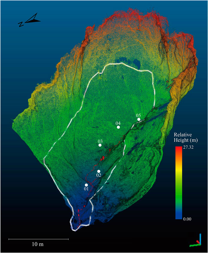
FIGURE 2. A three-dimensional perspective view of the gully point cloud on December 24, 2014, illustrating nearly vertical gully headwall and sidewalls. The white dots represent the scan locations and the dash red line represents the stream line of the gully bottom. The white polygon represents the boundary of the gully chancel, which is the focused area of the analysis.

We used the DEM of Difference (DoD) method to determine the topographic change within the gully channel from December 24, 2014 to February 8, 2015. This method calculates the elevation difference (ΔDEM) between a later DEM and an earlier DEM on a cell by cell basis (James et al., 2007; Wheaton, 2008; Wheaton et al., 2010; Croke et al., 2013; Lu et al., 2019):

$\Delta \text{DEM}={\text{DEM}}_2-{\text{DEM}}_1\pm \epsilon (1)$

where DEM₁ and DEM₂ are the DEMs produced by the first and the second times, respectively, in a time series, and ε is the propagated error of the change detection. ε is related to the errors associated with the scanner unit and the within- and between-survey registration of the DEMs in the time series.

Assuming each TLS survey obtained a set of ground points on a given cell of a DEM, the mean elevation of these points represents the elevation of the DEM cell and the standard deviation can be treated as the uncertainty (error) of the elevation measurement on this cell (just like we repeatedly measure the length of a table and then use the mean as the table length measurement and the standard deviation as the error of the measurement). For a DoD analysis of two DEMs generated by TLS scans in a time series, the error (ε) of the elevation difference at each cell can be propagated as:

$\epsilon =\sqrt{{\sigma }_1^2+{\sigma }_2^2}(2)$

where σ₁ and σ₂ are the standard deviations of the ground point elevations on a cell of the two DEMs in the time series, respectively. To determine the confidence level of the elevation difference, we calculated the Student’s t-score at each cell of the ΔDEM, following the method introduced by Wheaton (2008) and Wheaton et al. (2010):

$t=\frac{\left|z_{{\text{DEM}}_2}-z_{{\text{DEM}}_1}\right|}{\sqrt{{\sigma }_1^2+{\sigma }_2^2}}$ (3)

where $Z_{{\text{DEM}}_2}$ and $Z_{{\text{DEM}}_1}$ are the elevations of the two DEMs at a cell. The Student’s t distribution is close to a normal distribution when large number of points are used in the calculation and the confidence level of the elevation difference can be determined by the t-score at each cell (Wheaton, 2008; Wheaton et al., 2010). In this paper, we only consider the elevation change at and above the 95% confidence level (t = 1.96; p = 0.05).

The output of DEM of Difference, ΔDEM, is a raster with the value of each cell representing the elevation change: the changes within the uncertainty (95% confidence level) indicate no change, positive values larger than the uncertainty suggest deposition, and negative values smaller than the uncertainty represent erosion. The net volume change is estimated by (Lu et al., 2019):

$\text{Net}\text{Volume}={\displaystyle \sum \left(A_i\ast \Delta Z_i\right)}(4)$

where ΔZ_i is the elevation change (m) of a cell i (deposition: positive change; erosion: negative change) and A_i is the area (m²) of the cell i. The volumes of erosion and deposition can also be estimated by calculating negative and positive elevation changes separately. The DoD analysis and the volume calculation were performed using ArcGIS 10.6. To enhance the visualization, we overlaid the DEM and ΔDEM transparently (40%) with the DEM hillshading raster in ArcGIS. We also used the profile tool in ArcGIS to examine the morphological changes of a set of cross-sections and a longitudinal stream profile along the gully channel.

Analysis of the Effect of Digital Elevation Model Resolution on Area/Volume Estimates

The effect of DEM resolution on estimated changes in area and volume within the pool gully was investigated by generating a set of DEMs at cell resolutions from 0.02- to 0.66-m with an increment of 0.02-m based on the resampling of the original point clouds for these two surveys. The point clouds were divided into different cell sizes and all points within each cell were used to derive the elevation (mean) and uncertainty (standard deviation) of the DEM at each cell. We did not resample the datasets using the finest 0.02-m DEM because it may introduce errors due to the use of different resampling methods and parameters. This produced 33 DEMs of the gully channel for each survey date (a total of 66 DEMs). A raster of elevation uncertainty (error) was also derived for each DEM based on the standard deviation of the points within each cell of the DEM. Subsequently, a total of 33 ΔDEMs were produced to derive the areas/volumes of erosion and deposition at different resolutions. The relationship between DEM resolutions and derived erosion and deposition areas/volumes was then visually examined to assess the impact of the DEM resolution on the estimated areas/volumes of erosion and deposition, as well as on the interpretation of gully erosion-deposition processes. For illustration purposes, we also plotted the distribution maps and histograms of the erosion and deposition areas/volumes derived using DEM resolutions of 2-, 4-, 8-, 16-, 32- and 64-cm to show the effect of DEM resolution on estimated erosion and deposition areas/volumes.

Results

Gully Digital Elevation Models and Topographic Change

Figures 3A,B illustrate the 2-cm resolution DEMs of the TLS surveys on December 24, 2014 and February 8, 2015, respectively. The relative relief of the gully channel is about 17.9 m. Even after removing most of the vertical angle gully headwall and sidewalls, some steep areas remain on the eastern side of the gully (close to the gully head).

FIGURE 3

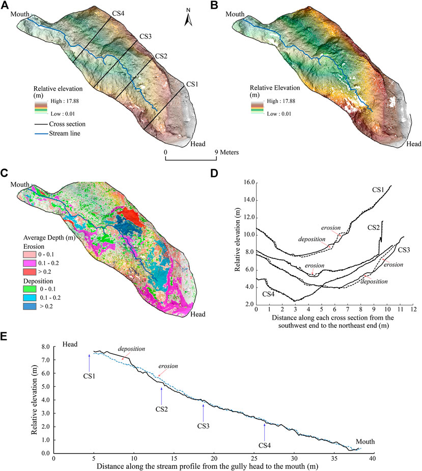
FIGURE 3. (A) The 2-cm resolution DEM of the gully channel for the TLS survey on December 24, 2014. (B) The 2-cm resolution DEM of the gully channel for the TLS survey on February 8, 2015. (C) The erosion and deposition spots within the gully channel generated by the difference of the two 2-cm DEMs on December 24, 2014 and February 8, 2015. (D) Four cross sections (locations marked in Panel A) along the gully to represent the topographic change between the survey period. (E) The longitudinal stream profile illustrating the pattern of erosion and deposition along the gully bottom. The dashed and solid lines in (D, E) represent the earlier and later DEM surfaces, respectively.

The difference of the highest resolution (2-cm) DEMs in these two survey dates yields the volume of change of 11.0 m³ of erosion and 8.2 m³ of deposition (at 95% confidence level). The net volume change is 2.8° m³ over the 46-day period, indicating a net loss of sediment from the gully channel (Table 2). Figure 3C illustrates the distribution of the erosion and deposition within the gully channel. The erosion spots are mainly distributed close to the gully headwall and sidewalls, whereas the deposition spots are mainly close to the channel and most deposition spots are just downslope the erosion spots (Figure 3C).

TABLE 2

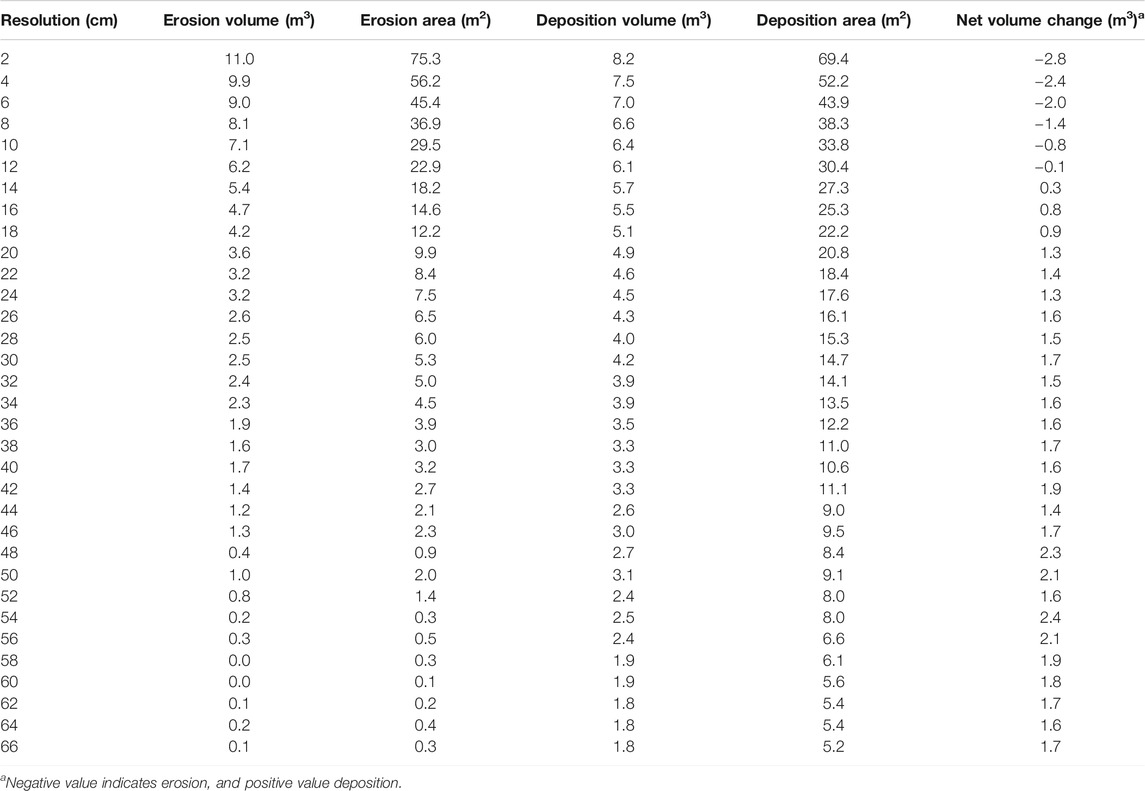
TABLE 2. The estimated erosion, deposition, and net changes of the gully channel based on the ΔDEMs at different resolutions.

Figure 3D illustrate the detailed morphological changes along the four cross-sections (CS1–CS4 marked in Figure 3A) of the gully channel. The dashed and solid lines represent the cross sections from the earlier and later DEMs, respectively. CS1 is close to the gully head and shows massive (10–20 cm in thickness) erosion of sediment on the eastern sidewall and its deposition toward the center of the gully channel, indicating a major sidewall failure occurred during this short period. The western side also shows some minor erosion and deposition. Down the gully, CS2 shows a major incision in the gully center, whereas the changes on both gully sides are minor. Further down the gully, CS3 shows a major sidewall erosion (>20 cm in thickness) on the eastern side of the gully followed with substantial deposition at the base of the erosion site. The western side of this cross section also shows some minor erosion and deposition spots. The cross section close to the outlet of the gully (CS4) is relatively stable and only has some minor changes on the western side. The longitudinal stream profile (Figure 3E) show most erosion and deposition occurred along the upper half of the gully bottom within ∼17 m from the gully head. Massive deposition occurred near the bottom of the gully head (close to CS1 and <10 m away from the gully head) and then erosion became dominated on the bottom (CS2 is in this section). The lower half of the gully bottom (>17 m from the gully head) were relatively stable with some minor erosion and deposition spots along the profile. It seems that the deposition at the base of the major sidewall erosion on the eastern side of CS3 had not reached the gully bottom. The morphological changes of these cross sections and the longitudinal stream profile provide a snapshot of sediment dynamics within the gully channel that was dominated by sidewall failure and deposition of the sediments at the base of the failure sites.

Digital Elevation Model Resolution Effect on Erosion and Deposition

A total of 33 DEM differences (ΔDEMs) were produced with resolutions from 0.02- to 0.66-m. Both estimated areas and volumes of erosion and deposition reduce with the increasing cell resolution (Table 2; Figure 4). The area and volume of erosion reduce relatively rapidly compared to those of deposition. The area of erosion is larger than that of deposition when the resolution is <8 cm, whereas the area of deposition becomes larger after the resolution is >8 cm (Figure 4A). Similarly, the net volume change is negative (erosion > deposition) when the resolution is finer than approximately 12 cm, whereas it becomes positive (deposition > erosion) after the resolution is coarser than 12 cm (Figure 4B). It seems that deposition becomes more dominant than erosion after the resolution is reduced to approximately 12 cm or coarser within the gully channel.

FIGURE 4

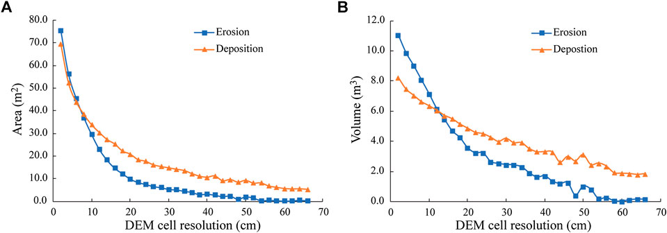
FIGURE 4. Relationships between derived areas (A) and volumes (B) of erosion and deposition and DEM resolutions with the propagation of elevation uncertainty.

Figure 5 provides the detailed distribution maps of DoD-derived erosion and deposition spots for DEM resolutions of 2-, 4-, 8-, 16-, 32-, and 64-cm. This figure also illustrates relatively rapid decrease in the erosion than the deposition spots toward coarser DEM resolutions, and it seems that the deposition becomes more apparent for coarser DEM resolutions (Figures 5D–F).

FIGURE 5

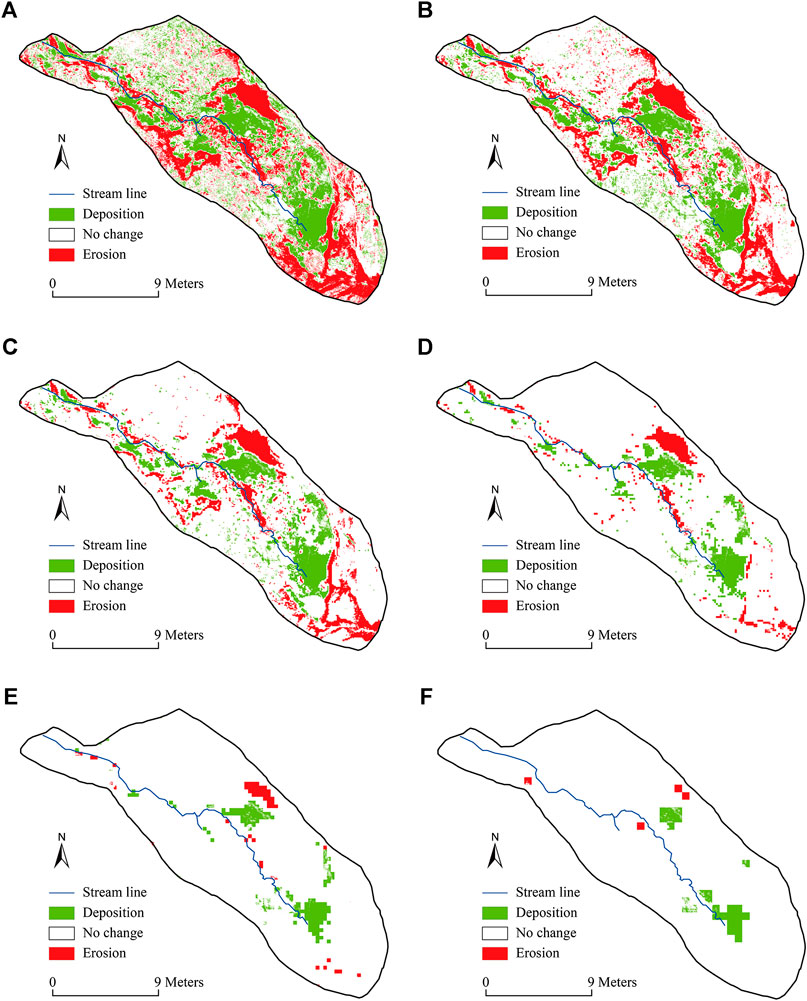
FIGURE 5. Spatial distribution of the erosion and deposition spots based on the DoD analysis for different DEM resolutions: (A) 2-cm, (B) 4-cm, (C) 8-cm, (D) 16-cm, (E) 32-cm, and (F) 64-cm.

Discussion

Topographic Change Detection

Visual interpretation of the ΔDEMs during the 46-days survey period suggests that most observed topographic changes are from mass wasting of the headwall and sidewalls. As illustrated in Figure 3C, the erosion spots generally correspond to the steep slope areas. The deposition spots are predominately located beneath the eroded areas. The cross-section analysis also demonstrated that mass wasting is the dominant process in this gully (Figure 3D). Specifically, CS1 and CS3 show the collapse of the sidewall and the deposition of the collapsed sediment at the foot of the collapse sites, representing the unstable phase of widening and infilling (Bocco, 1991; Morgan, 1996). In contrast, the steep eastern side of CS2 is relatively stable during this 46-day period and the erosion mainly occurs along the gully center. CS4 is relatively stable along the whole cross section with only some minor erosion and deposition on the western side. These cross sections likely represent snapshots of unstable gully development: the currently collapsed sidewalls in CS1 and CS3 may be stable for a while, whereas the relatively stable sidewalls in CS2 and CS4 may be collapsed in the next period. In addition, CS1 and CS3 show unevenly distributed topographic changes: major mass failures and sediment depositions on the eastern side, while the western side only has minor changes. The uneven topographic changes between the two sides may lead to the migration of the gully (Bocco, 1991), as it widens disproportionately in one direction over the other (Imeson and Kwaad, 1980; Bocco, 1991). This observation is consistent with previous studies, indicating that mass wasting is a random and repeating process within gullies where collapse of the head- and sidewalls leads to temporary local stabilization and an excess of sediment that is gradually expelled from the channel (Bennett, 1928; Ireland et al., 1939; Morgan, 1996). Note that sediment dynamics are also affected by the locations and current stages of the cross sections. The morphological change along the longitudinal stream profile (Figure 3E) suggests that erosion and deposition are more active in the upper gully. CS1 is located in the active part of the upper gully, and it could have more collapses in the next period. In contrast, CS4 is close to the mouth of the gully with more exposure of the terrace deposits under the surficial loess units. It may be relatively stable in the next period.

Digital Elevation Model Resolution Effect on Erosion and Deposition

The area and volume of erosion and deposition derived using DoD are affected by the DEM resolution. Our results show that both the estimated areas and volumes of erosion and deposition reduce with the coarsening cell resolution, but the area and volume of erosion reduce relatively rapidly than those of deposition (Figures 4, 5).

We hypothesize that the decreasing trends in erosion and deposition areas/volumes toward coarser resolutions are related to the method that we used to determine the propagated error in the DoD analysis (Eq. 3), and the relatively rapid smoothing of erosion is due to the different distributions of the erosion and deposition spots on slopes. To test these hypotheses, we plotted the histograms of erosion and deposition with and without the consideration of propagated error in the DoD analysis for different DEM resolutions of 2-, 4-, 8-, 16-, 32-, and 64-cm (Figure 6).

FIGURE 6

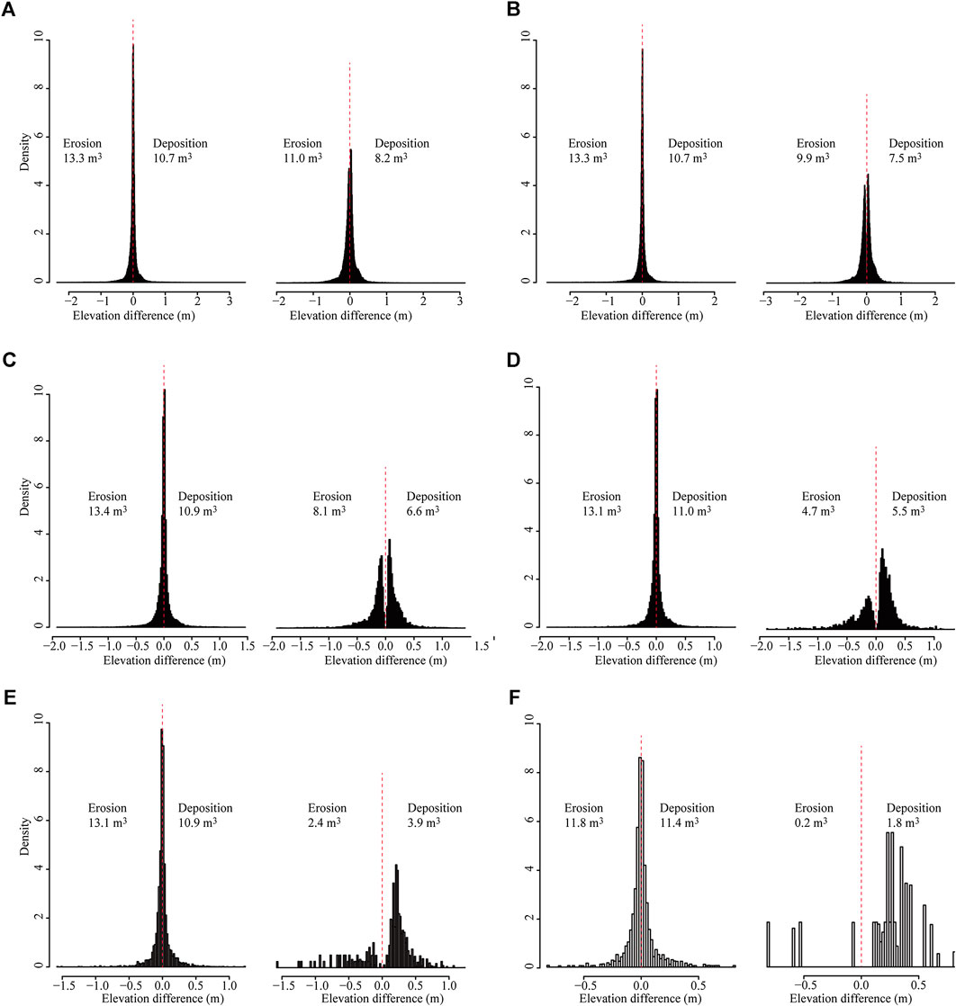
FIGURE 6. Histograms of the elevation difference representing erosion (negative elevation difference) and deposition (positive elevation difference) for different DEM resolutions: (A) 2-cm, (B) 4-cm, (C) 8-cm, (D) 16-cm, (E) 32-cm, and (F) 64-cm. The left histogram in each panel is for the direct DEM differencing without the consideration of errors. The right histogram in each panel is for the DoD analysis with the consideration of the propagated error based on Eq. 3.

The left histogram in each panel of Figure 6 is the result from DEM difference without considering the error. All resulted histograms are close to a normal distribution with more values close to zero (very small elevation change), indicating that both erosion and deposition areas/volumes derived using this approach include a significant contribution of very small elevation changes between the two DEMs that are probably caused by errors. Therefore, the erosion and deposition areas/volumes are overestimated using DEM difference without the consideration of the error. It is interesting though that the overestimated volumes of the erosion and deposition using this approach are relatively stable across different DEM resolutions.

The right histogram in each panel of Figure 6 is the result for the DoD analysis with the consideration of the propagated error based on Eq. 3. These histograms are mostly bimodal distributed, and the values close to zero (very small elevation change) are removed from the erosion and deposition calculation. The derived erosion and deposition areas/volumes are likely more realistic using this approach because most removed values with very small elevation changes in ΔDEM are likely caused by the measurement error. However, the ignored cells with small elevation changes that are less than the propagated error tend to increase toward coarser resolutions, resulting in the apparent decreases in the estimated erosion and deposition areas/volumes. This is because the error was estimated using the standard deviation of the elevation points within a DEM cell (Eqs 2 and 3) and a larger cell size in the rugged DEM like our studied gully tends to have a higher standard deviation in the TLS-collected elevation points, enhancing the smoothing effect for the estimated erosion and deposition toward coarser DEM resolutions.

Similar to Figure 4 and 5, Figure 6 also illustrates that the smoothing effect for the erosion part is more significant than the deposition toward coarser resolutions. Further investigation indicates that erosion occurs mainly on steep slopes, whereas deposition occurs on gentle slopes (Figure 7A). The propagated error (standard deviation in elevation points) used in the DoD analysis is positively related to the slope, leading to relatively higher propagated errors applied on steep slopes (Figure 7B). It is likely that this treatment filters more erosion than deposition spots, so that the erosion spots were smoothed rapidly toward coarser resolutions.

FIGURE 7

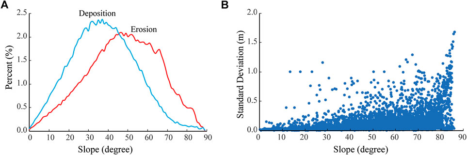
FIGURE 7. (A) The frequency distributions of erosion and deposition spots on different slopes. (B) The relationship between the uncertainty (standard derivation) of the DEM elevation and the slope.

In summary, the different smoothing behaviors of erosion and deposition we observed in this study are likely resulted from the biased propagated error incorporated in the DoD analysis because erosion and deposition are dominated on different slopes. This bias may make the deposition apparently more dominated toward coarser DEM resolutions (approximately 12 cm or coarser for volume estimate in this study), potentially misleading the interpretation of the erosion-deposition dynamics within the gully.

Conclusions

We investigated the pattern of short term erosion and deposition within an active gully in the Meeman-Shelby Forest State Park, west Tennessee, based on two TLS scans over a 46-day period in 2014–2015. The estimated volumes of erosion and deposition were 11.0 and 8.2 m³, respectively, with a net loss of 2.8 m³ of sediment (at the 95% confidence level) based on the 2-cm DEMs generated from the TLS surveys. This gully was mainly dominated by mass wasting of the headwall and sidewalls in this short period.

Both the estimated areas and volumes of erosion and deposition reduce with the increasing cell resolution. The estimated area and volume of erosion reduce relatively rapidly than those of deposition, likely caused by the fact that erosion spots occur on steep slopes with relatively high elevation standard deviations that are incorporated as propagated errors in the DoD analysis, so that they can be smoothed rapidly toward coarser resolution. In contrast, deposition spots are distributed on relatively gentle slopes with relatively low elevation standard deviations. These spots can be preserved relatively well toward coarser resolutions. The difference in the smoothing behaviors makes the deposition apparently more dominated after the resolution is reduced to a certain value, may causing an erroneous interpretation of gully erosion and deposition dynamics. Caution should be used, and higher resolution of the elevation data is recommended to quantify the erosion-deposition processes within the gully system.

Data Availability Statement

The datasets presented in this study can be found in online repositories. The names of the repository/repositories and accession number(s) can be found below: https://doi.org/10.6084/m9.figshare.12915347.v1

Author Contributions

YL and JM designed the research. YL, JM, and RW wrote the manuscript. JM and YL performed the research. YL, JM, and RW analyzed the data. All authors read and approved the final manuscript.

Funding

This work is supported by the US Environmental Protection Agency Small Urban Water Grant (Grant No. UW-00D45316) and the Stewart K. McCroskey Memorial Fund of the Department of Geography, University of Tennessee.

Conflict of Interest

The authors declare that the research was conducted in the absence of any commercial or financial relationships that could be construed as a potential conflict of interest.

Acknowledgments

We thank Rebecca Potter, Yanan Li, Xiaoyu Lu, and Makhan Virdi for feedback and technical support and John Schwartz for help on the early version of this manuscript. We would like to thank the Associate Editor, David K. Wright, and two reviewers for their constructive comments and suggestions to improve this paper.

References

Applied Imagery (2009). Quick terrain modeler. Chevy Chase, MD:Applied Imagery.

Google Scholar

Bangen, S. G., Wheaton, J. M., Bouwes, N., Bouwes, B., and Jordan, C. (2014). A methodological intercomparison of topographic survey techniques for characterizing wadeable streams and rivers. Geomorphology 206, 343–361. doi:10.1016/j.geomorph.2013.10.010

CrossRef Full Text | Google Scholar

Barnhardt, M. (1988a). Recent gully activity in Meeman-Shelby State Park Southwest Tennessee, USA. J. Tenn. Acad. Sci. 63, 61–64.

Google Scholar

Barnhardt, M. (1988b). Historical sedimentation in west Tennessee gullies. Southeast. Geogr. 281, 18–31. doi:10.1353/sgo.1988.0019

Google Scholar

Barnhardt, M. (1989). A 50-year-old gully reclamation project revisited. J. Soil Water Conserv. 44, 562–565.

Google Scholar

Bennett, H. H. (1928). The geographical relation of soil erosion to land productivity. Geogr. Rev. 18, 579–605. doi:10.2307/207949

CrossRef Full Text | Google Scholar

Betts, H. D., Trustrum, N. A., and Rose, R. C. D. (2003). Geomorphic changes in a complex gully system measured from sequential digital elevation models, and implications for management. Earth Surf. Process. Landf. 28, 1043–1058. doi:10.1002/esp.500

CrossRef Full Text | Google Scholar

Bocco, G. (1991). Gully erosion: processes and models. Prog. Phys. Geogr. Earth Environ. 15, 392–406. doi:10.1177/030913339101500403

CrossRef Full Text | Google Scholar

Bull, L. J., and Kirkby, M. J. (1997). Gully processes and modelling. Prog. Phys. Geogr. Earth Environ. 21, 354–374. doi:10.1177/030913339702100302

CrossRef Full Text | Google Scholar

Carr, S., Douglas, B., and Crosby, C. (2013). Terrestrial laser scanning (TLS) field camp manual. Boulder, CO: UNAVCO, 5–7.

Google Scholar

Cavalli, M., Tarolli, P., Marchi, L., and Dalla Fontana, G. D. (2008). The effectiveness of airborne LIDAR data in the recognition of channel-bed morphology. Catena 73, 249–260. doi:10.1016/j.catena.2007.11.001

CrossRef Full Text | Google Scholar

Challis, K. (2006). Airborne laser altimetry in alluviated landscapes. Archaeol. Prospect. 13, 103–127. doi:10.1002/arp.272

CrossRef Full Text | Google Scholar

Charrier, R., and Li, Y. (2012). Assessing resolution and source effects of digital elevation models on automated floodplain delineation: a case study from the Camp Creek Watershed, Missouri. Appl. Geogr. 34, 38–46. doi:10.1016/j.apgeog.2011.10.012

CrossRef Full Text | Google Scholar

Corsini, A., Castagnetti, C., Bertacchini, E., Rivola, R., Ronchetti, F., and Capra, A. (2013). Integrating airborne and multi-temporal long-range terrestrial laser scanning with total station measurements for mapping and monitoring a compound slow moving rock slide. Earth Surf. Process. Landf. 38, 1330–1338. doi:10.1002/esp.3445

CrossRef Full Text | Google Scholar

Croke, J., Todd, P., Thompson, C., Watson, F., Denham, R., and Khanal, G. (2013). The use of multi temporal LiDAR to assess basin-scale erosion and deposition following the catastrophic January 2011 Lockyer flood, SE Queensland, Australia. Geomorphology 184, 111–126. doi:10.1016/j.geomorph.2012.11.023

CrossRef Full Text | Google Scholar

Dai, W., Yang, X., Na, J., Li, J., Brus, D., Xiong, L., et al. (2019). Effects of DEM resolution on the accuracy of gully maps in loess hilly areas. Catena 177, 114–125. doi:10.1016/j.catena.2019.02.010

CrossRef Full Text | Google Scholar

Deng, Y., Wilson, J. P., and Bauer, B. O. (2007). DEM resolution dependencies of terrain attributes across a landscape. Int. J. Geogr. Inf. Sci. 21, 187–213. doi:10.1080/13658810600894364

CrossRef Full Text | Google Scholar

Dotterweich, M., Ivester, A. H., Hanson, P. R., Larsen, D. L., and Dye, D. H. (2014). Natural and human-induced prehistoric and historical soil erosion and landscape development in Southwestern Tennessee, USA. Anthropocene 8, 6–24. doi:10.1016/j.ancene.2015.05.003

CrossRef Full Text | Google Scholar

Downes, R. G. (1946). Tunnelling erosion in north-eastern Victoria. J. Council Sci. Ind. Res. 19, 283–292.

Google Scholar

FARO (2015). Faro scene (version 5.5). Lake Mary, FL: FARO.

Google Scholar

Gao, P. (2013). “Rill and gully development processes,” in Treatise on geomorphology. Editor J.F. Shroder (San Diego, CA: Academic Press). 122–131.

Google Scholar

Heede, B. H. (1976). Gully development and control: the status of our knowledge. Fort Collins, CO: Department of Agriculture, Forest Service, Rocky Mountain Forest and Range Experiment Station.

Google Scholar

Heritage, G., and Hetherington, D. (2007). Towards a protocol for laser scanning in fluvial geomorphology. Earth Surf. Process. Landf. 32, 66–74. doi:10.1002/esp.1375

CrossRef Full Text | Google Scholar

Höfle, B., Griesbaum, L., and Forbriger, M. (2013). GIS-based detection of gullies in terrestrial LiDAR data of the Cerro Llamoca peatland (Peru). Remote Sens. 5, 5851–5870. doi:10.3390/rs5115851

CrossRef Full Text | Google Scholar

Hohenthal, J., Alho, P., Hyyppä, J., and Hyyppä, H. (2011). Laser scanning applications in fluvial studies. Prog. Phys. Geogr. Earth Environ. 35, 782–809. doi:10.1177/0309133311414605

CrossRef Full Text | Google Scholar

Hudson, N. (1981). Soil conservation. 2nd Edn. New York, NY:Cornell University Press, 24–56.

Google Scholar

Imeson, A. C., and Kwaad, F. J. P. M. (1980). Gully types and gully prediction. Geogr. Tijdschr. 14, 430–441.

Google Scholar

Ireland, H. A., Sharpe, C. F. S., and Eargle, D. (1939). Principles of gully erosion in the Piedmont of South Carolina. Washington DC: U.S. Department of Agriculture.

Google Scholar

James, L. A. (2011). Contrasting geomorphic impacts of pre- and post-Columbian land-use changes in Anglo America. Phys. Geogr. 32 (5), 399–422. doi:10.2747/0272-3646.32.5.399

CrossRef Full Text | Google Scholar

James, L. A., Watson, D. G., and Hansen, W. F. (2007). Using LIDAR data to map gullies and headwater streams under forest canopy: South Carolina, USA. Catena 71, 132–144. doi:10.1016/j.catena.2006.10.010

CrossRef Full Text | Google Scholar

Knighton, D. (1998). Fluvial forms and processes: a new perspective. London: Arnold, 135.

Google Scholar

Kukko, A., Kaasalainen, S., and Litkey, P. (2008). Effect of incidence angle on laser scanner intensity and surface data. Appl. Opt. 47, 986–992. doi:10.1364/ao.47.000986

CrossRef Full Text | Google Scholar

Leopold, L. B., and Miller, J. P. (1956). Ephemeral streams: hydraulic factors and their relation to the drainage net. Washington, DC: U.S. Govt. Print.

Google Scholar

Li, Y. K. (2015). Effects of analytical window and resolution on topographic relief derived using digital elevation models. GISci. Remote Sens. 52, 462–477. doi:10.1080/15481603.2015.1049577

CrossRef Full Text | Google Scholar

Lohani, B., and Mason, D. C. (2001). Application of airborne scanning laser altimetry to the study of tidal channel geomorphology. ISPRS J. Photogramm. Remote Sens. 56, 100–120. doi:10.1016/s0924-2716(01)00041-7

CrossRef Full Text | Google Scholar

Lu, X., Li, Y., Washington-Allen, R. A., Li, Y., Li, H., and Hu, Q. (2017). The effect of grid size on the quantification of erosion, deposition, and rill network. Int. Soil Water Conserv. Res. 5, 241–251. doi:10.1016/j.iswcr.2017.06.002

CrossRef Full Text | Google Scholar

Lu, X., Li, Y., Washington-Allen, R. A., and Li, Y. (2019). Structural and sedimentological connectivity on a rilled hillslope. Sci. Total Environ. 655, 1479–1494. doi:10.1016/j.scitotenv.2018.11.137

CrossRef Full Text | Google Scholar

Milan, D. J., Heritage, G. L., and Hetherington, D. (2007). Application of a 3D laser scanner in the assessment of erosion and deposition volumes and channel change in a proglacial river. Earth Surf. Process. Landf. 32, 1657–1674. doi:10.1002/esp.1592

CrossRef Full Text | Google Scholar

Morgan, R. P. C. (1996). Soil erosion and conservation. 2nd edn. Harlow:Longman, 213.

Google Scholar

Nearing, M. A., Norton, L. D., Bulgakov, D. A., Larionov, G. A., West, L. T., and Dontsova, K. M. (1997). Hydraulics and erosion in eroding rills. Water Resour. Res. 33, 865–876. doi:10.1029/97wr00013

CrossRef Full Text | Google Scholar

Perroy, R. L., Bookhagen, B., Asner, G. P., and Chadwick, O. A. (2010). Comparison of gully erosion estimates using airborne and ground-based LiDAR on Santa Cruz Island, California. Geomorphology 118, 288–300. doi:10.1016/j.geomorph.2010.01.009

Google Scholar

Picco, L., Mao, L., Cavalli, M., Buzzi, E., Rainato, R., and Lenzi, M. A. (2013). Evaluating short-term morphological changes in a gravel-bed braided river using terrestrial laser scanner. Geomorphology 201, 323–334. doi:10.1016/j.geomorph.2013.07.007

Google Scholar

Poesen, J. (1993). “Gully topology and gully control measures in the European loess belt,” in Farm land erosion in temperate plains environment and hills. Editors S. Wicherek (Amsterdam: Elsevier), 221–239.

Google Scholar

Poesen, J., Nachtergaele, J., Verstraeten, G., and Valentin, C. (2003). Gully erosion and environmental change: importance and research needs. Catena 50, 91–133. doi:10.1016/s0341-8162(02)00143-1

CrossRef Full Text | Google Scholar

Poesen, J., Vandaele, K., and Van Wesemael, B. (1998). “Gully erosion: importance and model implications,” in Modeling soil erosion by water. Editors J. Boardman and D.T. Favis-Mortlock (Berlin: Springer), 285–311.

Google Scholar

Poesen, J., Vanwalleghem, T., de Vente, J., Knapen, A., Verstraete, G., and Martinex-Casasnovas, J. A. (2006). “Gully erosion in Europe,” in Soil erosion in Europe. Editors J. Boardman and J. Poesen (Chichester: Wiley), 515–536.

Google Scholar

Rodbell, D. T., Forman, S. L., Pierson, J., and Lynn, W. C. (1997). Stratigraphy and chronology of Mississippi Valley loess in western Tennessee. Geol. Soc. Am. Bull. 109, 1134–1148. doi:10.1130/0016-7606(1997)109<1134:sacomv>2.3.co;2

CrossRef Full Text | Google Scholar

Sease, E. C., Flowers, R. L., Mangrum, W. C., and Moore, R. K. (1970). Soil survey—Shelby County Tennessee. Washington, DC: United States Department of Agriculture, Soil Conservation Service.

Google Scholar

Tennessee State Parks (2016). Tennessee Department of Environment and Conservation. Available at: http://tnstateparks.com/parks/about/meeman-shelby (Accessed March 9, 2016).

Google Scholar

Thompson, J. A., Bell, J. C., and Butler, C. A. (2001). Digital elevation model resolution: effects on terrain attribute calculation and quantitative soil-landscape modeling. Geoderma 100, 67–89. doi:10.1016/s0016-7061(00)00081-1

CrossRef Full Text | Google Scholar

Trimble, S. W. (1974). Man-induced soil erosion on the Southern Piedmont: 1700–1970. Ankeny, IA: Soil Conservation Society of America.

Google Scholar

Trimble, S. W. (1985). Perspectives on the history of soil erosion control in the Eastern United States. Agric. Hist. 59, 162–180.

Google Scholar

US Climate Data (2016). U.S. Weather Service. Available at: http://www.usclimatedata.com (Accessed March 9, 2016).

Google Scholar

Vittorini, S. (1972). The effect of soil erosion in an experimental station in the Pliocene clay of the Val d’Era (Tuscany) and its influence on the evolution of the slopes. Acta Geogr. Debrecina. 10, 71–81.

Google Scholar

Wheaton, J. M. (2008). Uncertainty in morphological sediment budgeting of rivers. Southampton, United Kingdom: PhD University of Southampton.

Google Scholar

Wheaton, J. M., Brasington, J., Darby, S. E., and Sear, D. A. (2010). Accounting for uncertainty in DEMs from repeat topographic surveys: improved sediment budgets. Earth Surf. Process. Landforms. 35, 136–156

Google Scholar

Wolock, D. M., and Price, C. V. (1994). Effects of digital elevation model map scale and data resolution on a topography-based watershed model. Water Resour. Res. 30, 3041–3052. doi:10.1029/94wr01971

CrossRef Full Text | Google Scholar

Woolard, J. W., and Colby, J. D. (2002). Spatial characterization, resolution, and volumetric change of coastal dunes using airborne LiDAR: Cape Hatteras, North Carolina. Geomorphology 48, 269–287. doi:10.1016/s0169-555x(02)00185-x

CrossRef Full Text | Google Scholar

Yang, P., Ames, D. P., Fonseca, A., Anderson, D., Shrestha, R., Glenn, N. F., et al. (2014). What is the effect of lidar-derived DEM resolution on large-scale watershed model results? Environ. Model. Softw. 58, 48–57 doi:10.1016/j.envsoft.2016.04.026

CrossRef Full Text | Google Scholar

Young, A. P., Olsen, M. J., Driscoll, N., Flick, R. E., Gutierrez, R., Guza, R. T., et al. (2010). Comparison of airborne and terrestrial LiDAR estimates of seacliff erosion in southern California. Photogramm Eng. Remote Sens. 76, 421–427. doi:10.14358/pers.76.4.421

CrossRef Full Text | Google Scholar

Zhang, W., and Montgomery, D. R. (1994). Digital elevation model grid size, landscape representation, and hydrologic simulations. Water Resour. Res. 30, 1019–1028. doi:10.1029/93wr03553

CrossRef Full Text | Google Scholar

Zhu, T. X. (2003). Tunnel development over a 12 year period in a semi-arid catchment of the Loess Plateau, China. Earth Surf. Process. Landf. 28, 507–525. doi:10.1002/esp.455

CrossRef Full Text | Google Scholar