 Elke Schneebeli-Hermann
- Paleontological Institute and Museum, University of Zurich, Zurich, Switzerland
The Early Triassic was one of the most remarkable time intervals in Earth History. To begin with, life on Earth had to face one of the largest subaerial volcanic degassing, the Siberian Traps, followed by a plethora of accompanying environmental hazards with pronounced and repeated climatic changes. These changes not only led to repeated and, for several marine nektonic clades, intense extinction events but also to significant changes in terrestrial ecosystems. The Early Triassic terrestrial ecosystems of the southern subtropical region (Pakistan) are not necessarily marked by abrupt extinction events but by extreme shifts in composition. Modern ecological theories describe such shifts as catastrophic regime shifts. Here, the applicability of modern ecological theories to these past events is tested. Abrupt shifts in ecosystems can occur when protracted changing abiotic drivers (e.g. climate) reach critical points (thresholds or tipping points) sometimes accentuated by stochastic events. Early Triassic terrestrial plant ecosystem changes stand out from the longer term paleobotanical records because changes of similar magnitude have not been observed for many millions of years before and after the Early Triassic. To date, these changes have been attributed to repeated severe environmental perturbations, but here an alternative explanation is tested: the initial environmental perturbations around the Permian–Triassic boundary interval are regarded here as a main cause for a massive loss in terrestrial ecosystem resilience with the effect that comparatively small-scale perturbations in the following ∼5 Ma lead to abrupt regime shifts in terrestrial ecosystems.
Introduction
Sediments – the Earth history archive – reveal their mysteries only bit by bit. Thus, the narrative of momentous and complex events in the remote past of system Earth significantly changes as knowledge accumulates. The research history of the biotic and abiotic events around the Permian–Triassic boundary and the subsequent Early Triassic exemplifies how complex the story can get.
About 52% of marine invertebrate and vertebrate families and ∼81% species went extinct across the Permian–Triassic boundary (Raup and Sepskoski, 1982; Stanley, 2016). The search for the culprit for this massive extinction of marine communities has included a long list of suspects, such as sea level regression (Holser et al., 1989), massive volcanic activity (Renne and Basu, 1991; Renne et al., 1995), ocean acidification caused by volcanic degassing (Heydari et al., 2008), global warming caused by CO2 (Wignall, 2001; Kidder and Worsley, 2004; Kiehl and Shields, 2005), oceanic anoxia (Wignall and Hallam, 1992; Wignall and Hallam, 1993; Wignall and Twitchett, 1996; Wignall and Twitchett, 2002; Grice et al., 2005; Kump et al., 2005), hypercapnia (Knoll et al., 1996) and an extra-terrestrial impact (Becker et al., 2004). In recent years, the plethora of possible triggers for the mass extinction has been narrowed down to the eruption of the Siberian Traps, associated with a succession of consequential environmental changes, some of them previously thought to be the sole responsible party (Sobolev et al., 2011; Wignall, 2011).
The precision of radiometric and biochronological dating of biotic and abiotic events across the Permian-Triassic boundary interval in various locations has increased enormously (Shen et al., 2011; Burgess et al., 2014; Brosse et al., 2016). While research on extinction severity and timing of events has increased, the research on biotic recovery has highlighted the complexity of biotic-abiotic interrelations especially in times of fragile ecosystems. For various marine groups, the mode and pattern of Early Triassic recovery has been elucidated. Benthic organisms show a rather prolonged gradual recovery with regional rapid recovery phases (Twitchett et al., 2004; Fraiser and Bottjer, 2005; Hautmann et al., 2011; Hofmann et al., 2014; Hautmann et al., 2015). In contrast, nektonic organisms suffered from repeated extinction and recovery events, which coincided with changes in carbon cycling (Brayard et al., 2006; Orchard, 2007; Brayard et al., 2009; Algeo et al., 2019). Changes in terrestrial tetrapod faunas across the Permian–Triassic transition were also documented from various regions (e.g. Benton et al., 2004; Ward et al., 2005). However, the coincidence of marine and continental faunal collapse is still controversial (Benton et al., 2004; Lucas, 2009; Gastaldo et al., 2015; Gastaldo et al., 2020). Thus, the animal Permian–Triassic story changed from an easy to digest novel that could be entitled “sudden severe biodiversity loss followed by prolonged recovery” to a grave voluminous trilogy if not an entire series full of previously unexpected bends.
Like the animal extinction-tale, the Permian–Triassic boundary tale for plants has become rather complex over the last decades. Previously, it has been supposed that a similar extinction severity and recovery pattern as for benthic organisms applies for land plants (Retallack, 1995; Visscher et al., 1996; Looy et al., 2001; McElwain and Punyasena, 2007; Benton and Newell, 2014; Cascales-Miñana et al., 2016). However, depending on the type of fossil that is studied (macro-vs microfossils), geographic position of study location, time resolution of fossil findings and type of analysis indicate either a severe loss of standing biomass (Fielding et al., 2019) or inexistence of abrupt diversity decline of land plants (Schneebeli-Hermann et al., 2017). Currently, two different connotations of the term mass extinction appear to cause seemingly opposing views on the Permian–Triassic events. On the one hand, mass extinction is associated with the loss of biomass as documented for example in the Sydney Basin (Mays et al., 2020; Vajda et al., 2020) and on the other hand, with the loss in plant diversity, i.e. the taxonomic approach to mass extinction. The latter follows the original approach to mass extinction (Jablonski, 1986; Sepkoski, 1986) whereas the first one underlines the enormous impact of huge ecosystem restructuring on an array of biosphere-lithosphere-atmosphere cycles. A global compilation of macro- and microfossil data demonstrating no biodiversity loss across the Permian–Triassic transition (Nowak et al., 2019) contrasts with significant ecosystem changes reflected in the dominance structure of vegetation close to the Permian–Triassic boundary and thereafter (Hochuli et al., 2010a; Hermann et al., 2011a; Hochuli et al., 2016). The changes observed are repeated shifts from gymnosperm-dominated to pteridophyte (mainly lycophyte)-dominated plant communities. These occur in the first half of the Early Triassic (spanning ∼2.5 Myrs) commencing with the Permian–Triassic extinction event. However, these changes in dominance structure had precursory events, such as the collapse of the Glossopteris biome in the Sydney Basin of Australia (Mays et al., 2020) or the onset of Gigantopteris forest decline of Cathaysia (Chu et al., 2020). Although deep-time paleontological sampling cannot achieve the high data-density of modern ecological databases with automated monthly, daily or even hourly collected data, these shifts occur to be abrupt. Large abrupt shifts in modern ecosystems including terrestrial ecosystems have been ascribed to changes between alternative stable states (Scheffer et al., 2001; Scheffer and Carpenter, 2003; see short summary of this below). The loss of ecosystem resilience facilitates such critical regime shifts, driving mechanisms can be gradual environmental changes reaching a critical threshold, or stochastic events (Scheffer et al., 2001; Scheffer, 2009). For the Early Triassic, environmental changes are reflected in multiple carbon cycle perturbations (e.g. Payne et al., 2004) which are closely linked to the previously mentioned shifts in plant-community dominance structure (Hermann et al., 2011a).
Could the Early Triassic changes in vegetation pattern, as seen in the Lower Triassic palynological records of Pakistan, be described as catastrophic shifts between alternative regimes as documented for several modern ecosystems? Or, in other words, it will be tested, whether the alternative stable state theory is applicable to the Early Triassic palynology and isotope dataset despite of the shortcomings of a deep-time record. The palynological record from Pakistan will be examined for the presence of regime shifts using different data-driven methods (principle component analysis, sequential t-test, cluster analysis, etc.), thus avoiding a priori assumptions about presence and timing of possible regime shifts. The importance of paleoecological datasets for present-day efforts in conservation of biodiversity is frequently stressed (e.g. Willis et al., 2010). It is too far-fetched and not intended to regard the Early Triassic, a time interval ∼252 Myrs back in Earth history, influential for present-day conservation efforts. But, examining the Early Triassic vegetation patterns from a different angle might offer a different view on the events during this critical time in Earth history. Can biotic and abiotic processes be described which reduced or increased Early Triassic ecosystem resilience and the consequences thereof? Could changes in diversity potentially be a measure for assessing changes in resilience of a deep-time ecosystems?
Thus, the purpose of this essay is to offer a hypothetical explanation for Early Triassic terrestrial vegetation dynamics based on modern ecosystem regime shifts. It offers an alternative, non-catastrophic view on (terrestrial) ecosystem dynamics in a unique time interval in Earth history. This discussion begins with a brief overview of alternative stable states theory.
Materials and Methods
Regime Shifts in Ecosystems
Based on the understanding that observed ecosystem behavior could be characterized using theoretical models (Lewontin, 1969; Holling, 1973), May (1977) described the range of states an ecosystem could potentially occupy as dynamical landscapes with stable valleys and dividing (unstable) ridges (“hills and watersheds”). The “geographic” coordinates of this landscape are 1) species composition and their interactions and 2) environmental conditions (Figure 1). Thus, depending on the geography of the dynamical landscape there might be more than one possible stable configuration or regime for an ecosystem.
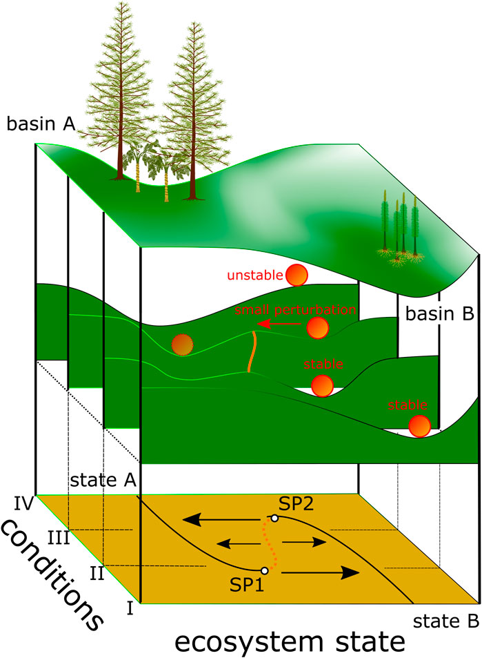
FIGURE 1. Dynamical landscape modified after Scheffer et al., 2001. Valleys or basins are areas of stable equilibria. Here, basin A represents gymnosperm-dominated vegetation, and basin B lycophyte-dominated vegetation. Changing conditions (steps I–IV) change the altitudinal differentiation or the geography and thus the resilience. Smaller additional perturbations can then drive plant communities over the remaining saddle (geographically) or toward the switch points (SP1 and SP2) from where the system drops to the contrasting state. Plant reconstructions: Tall tree in basin A represents a Triassic conifer Telemachus after Bomfleur et al. (2013), the smaller tree in basin A represents a medullosan seed fern after Stewart and Delevoryas (1956), and Pleuromeia after Fuchs et al. (1991) is illustrated in basin B.
The stability of an ecosystem in this landscape is continuously tested by gradual environmental changes. Responses of ecosystems to these incremental changes can differ from gradual or linear change to abrupt changes when certain thresholds are reached (Figure 1 e.g. geography for condition I) to a response with hysteresis (Figure 1 geography of condition III). In the latter, changing environmental conditions drive the system towards conditions II and thus close to switch point 1 (SP1), which represents a threshold (Figure 1) from where the system drops abruptly from one regime (stable state or valley) into the other. A return to the previous state requires restoration of conditions beyond switch point 1 (Figure 1).
Ecosystems have the capacity to absorb a certain amount of disturbance or repeated small perturbations without dramatic subsequent changes. This resilience in the dynamical landscape is the differential altitude between basins or valleys and the bordering hills. The higher the differential altitude, the more resilient an ecosystem is to perturbations. However, even if small scale perturbations might not trigger big immediate changes in an ecosystem, cumulatively they could change the position of the ecosystem in the dynamical landscape. i.e. the ecosystem might be positioned where reduced differential altitude between different valleys, i.e. reduced resilience of the ecosystem prevails (Scheffer et al., 2001).
Abrupt regime shifts in absence of a single large-scale perturbation have been documented to occur in various modern ecosystems (e.g. lakes, Scheffer, 1993; savannahs, Ludwig et al., 1997; coral reefs, McCook, 1999). The underlying changes in conditions in these modern examples have been identified to be changes in nutrient flux to lakes or orbitally forced solar radiation variations (Scheffer and Carpenter, 2003). Despite the growth of research in this field, it is still a challenge to prove the existence of multiple stable regimes (valleys) in ecosystems. However, the importance of paleoecological datasets is emphasized, in order to better understand combinations of biotic and abiotic processes supporting resilience (Willis et al., 2010). A first step in identifying regime shifts can be the visual inspection of time-series data. Abrupt shifts thus revealed might not necessarily indicate the presence of two or more regimes, as they might be the result of simple threshold response to a main driver of the ecosystem (Scheffer and Carpenter, 2003; Andersen et al., 2009). Therefore, abrupt changes in time-series data need to be tested further by statistical analysis such as principal component analysis and age-constrained cluster analysis (Andersen et al., 2009).
Basic Glossary
Ecological threshold: A point at which small changes in critical environmental drivers induce a regime shift.
Hysteresis: a system that has two stable states and that remains in a stable state configuration under changing conditions until a critical threshold is reached. There, the system switches abruptly to the second state. Conditions need to be restored beyond the first threshold in order to provoke a shift back to the first state.
Regime shift: abrupt change in ecosystem configuration when a certain threshold is passed. (Alternative terms: shifts between alternative stable states, alternative equilibria, or alternative attractors). The regimes or stable states are represented as valleys or basins in the dynamical landscape.
Resilience: The amount of environmental perturbation an ecosystem can absorb without shifting to a different regime.
The Vegetation Record
The deep time data set tested for the presence of regime shifts is a compilation of palynological data from three gorges in the Salt and Surghar Ranges in Pakistan (Amb, Nammal, and Chitta-Landu) (Figure 2). The sedimentary succession ranges from the upper Changhsingian into the Middle Triassic (Hermann et al., 2011a; Hermann et al., 2011b; Schneebeli-Hermann et al., 2015). Compared to localities where the Early Triassic palynofloral record is extremely poor, such as Central Europe, these localities offer unexpected perspectives on the vegetation dynamics during the Early Triassic due to their excellent organic matter preservation. The successions in Pakistan are characterized by a mixture of siliciclastic and carbonate lithologies deposited on the Tethyan margin of the Indian continental shelf. Changes in the palynological associations are unrelated to sea-level changes (Hermann et al., 2012) and stable sediment transport direction indicates no drastic change of the source area for sediment and sporomorph supply (Pakistani–Japanese Research Group 1985; Hermann et al., 2012).
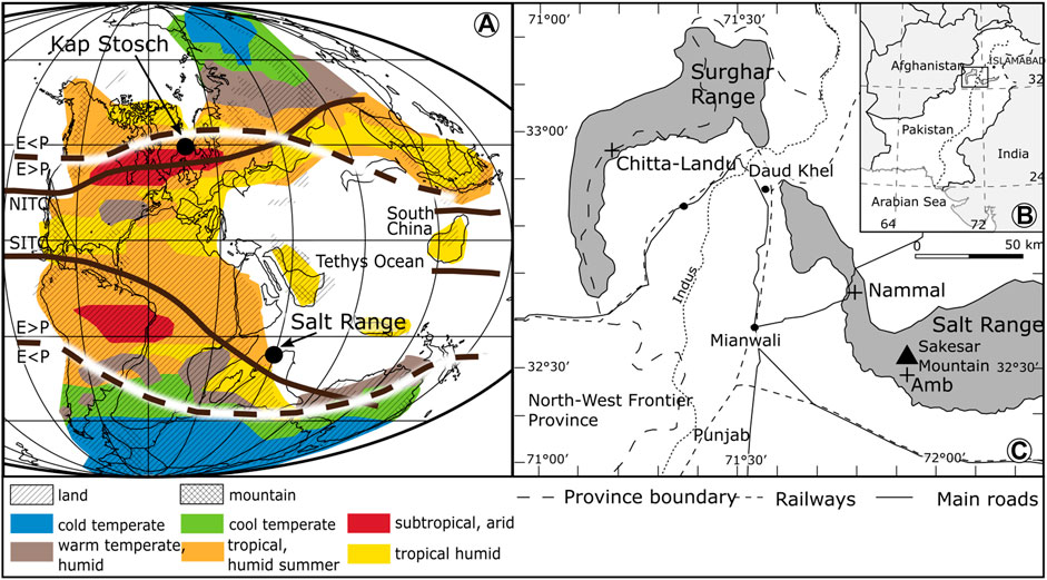
FIGURE 2. (A) Permian–Triassic Pangea paleogeography, modified after Smith et al. (1994). Precipitation/evaporation ratio (p < E, p > E) after Ziegler et al. (2003). Late Permian biomes and northern and southern intertropical convergence zones (NITC, SITC) modified after Kutzbach and Ziegler (1993). (B) Geographic position of the Salt Range in Pakistan, and (C) location of Nammal, Chitta-Landu, and Amb sections.
The palynological data of 106 samples from all three gorges was first adjusted to generic level and then grouped according to their botanical affinities (Balme, 1995; Lindström et al., 1997; Taylor et al., 2006; Traverse, 2007). The approach in reducing the data set to generic level is justified by the fact that using the species level for plant group assignment does not offer better resolution because the botanical affinity of species is seldom certainly known or known only in few cases. The relative abundances of plant groups are plotted against a composite log of the three succession (Figure 3). Remarkable are the prominent shifts between lycophyte-dominated vegetation in the Dienerian, middle Smithian, and a smaller interval within the Spathian and gymnosperm-dominated vegetation during the Permian, late Smithian, and the Anisian. The Griesbachian, early Smithian and most of the Spathian assemblages are marked by a mixed character yielding both plant types almost equally. A drawback of the Pakistan successions is that the Griesbachian (only three samples) is largely underrepresented.
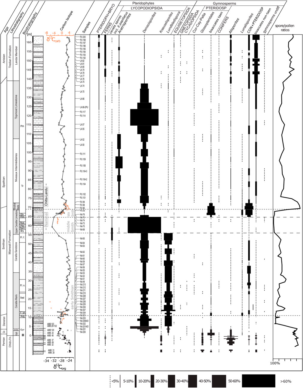
FIGURE 3. Plant associations based on relative abundances of fossil spore and pollen data from Nammal and Chitta Landu (Hermann et al., 2011a) and Amb (Schneebeli-Hermann et al., 2015). Biostratigraphy: ammonoids (Brühwiler, 2010; Ware 2015): Prh, Prohungarites beds; Tr, Tirolites beds; Gly, Glyptophiceras sinatum beds; Was, Wasatchites distractum beds; Nya, Nyalamites angustecostatus beds; Psc, Pseudoceltites multiplicatus beds; Nam, Nammalites pilatoides beds; Bry, Brayardites compressus beds; Fl. f., Flemingites flemingianus beds; Fl. n., Flemingites nanus beds; Xed, Xenodiscoides perplicatus beds; F. bh., Flemingites bhargavai beds; Prlb., Prionolobusrotundatus beds; Gyr, Gyronites beds; conodonts: asterisk depicts position of H.t.—Hindeous typicalis; H. pp.—Hindeous praeparvus; H. p.?—ambiguous specimen of Hindeodus parvus. Bulk organic carbon isotope data for Nammal and Chitta-Landu from Hermann et al. (2011b), for Amb: Light gray triangles: δ13C wood particles, gray squares: δ13C cuticles, black filled dots: bulk organic carbon δ13C. Schneebeli-Hermann et al. (2013). PTERIDOPH + BRYO, undifferentiated Pteridophytes and Bryophytes; Cor, Corystospermales; Cay, Caytoniales; Pelta, Peltaspermales; PTERIDOSP, pteridosperms; bisaccates taen, undifferentiated taeniate bisaccate pollen grains; CON + PTERIDOSP, undifferentiated conifers and pteridosperms.
Age Determination
The successions in Pakistan include the uppermost part of the Upper Permian Chiddru Formation, the Lower Triassic Mianwali Formation with Kathwai, Mittiwali, and Narmia Members, and the Middle Triassic Tredian Formation. Besides the Tredian Formation, these are biostratigraphically dated based on conodonts and ammonoids (Brühwiler, 2010; Goudemand, 2011; Ware, 2015). Ash beds for radiometric dating are not available. Thus, four radiometric ages from China (all measured with EARTHTIME tracer solution) were selected and correlated with the Pakistan composite log(Table 1) based on the assumption of constant depositional rates between two dates and that biostratigraphic and chemostratigraphic markers between Pakistan and China are not diachronous. Interpolation between two radiometric ages allowed assignment of a numerical age to each sample. A major drawback of this approach, is, that so far, no radiometric age for the Griesbachian–Dienerian boundary is available. Thus, the position of the Griesbachian–Dienerian boundary as shown in Figure 4 indicates that the first assumption of constant sedimentation rates can lead to false estimates with respect to the duration of stages. In Figure 4, the Griesbachian appears to be geochronologically very short (ca. 200 kyrs) because the boundary is drawn in the correct biostratigraphic position. However, sediment flux analysis from Kap Stosch, Greenland, demonstrates that the duration of Griesbachian (∼400 kyrs) and Dienerian (∼500 kyrs) are close to equal (Sanson-Barrera, 2016).

TABLE 1. Radiometric dates and their correlation with the Pakistan composite record.
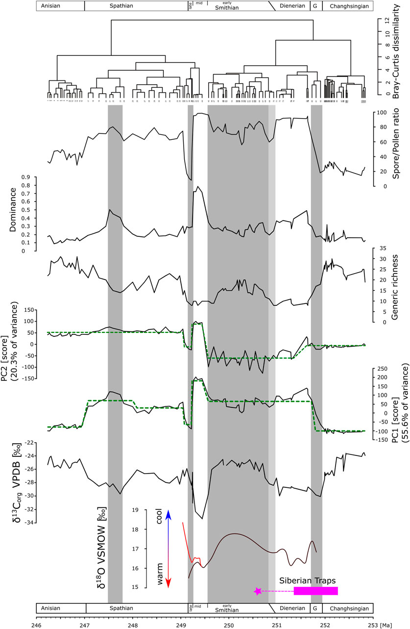
FIGURE 4. Time-series of carbon isotopes data, diversity and dominance analyses, principal component analysis, and cluster analysis. Green dashed lines in the PC1 and PC2 time-series represent shifts in the mean of the respective PC, derived by sequential t-test after Rodionov (2004). Conodont apatite oxygen isotope data modified after Romano et al. (2013) (black curve) and Goudemand et al. (2019) (red curve). Geochronology of Siberian Traps volcanic activity, main phase <1Myrs after Burgess and Bowring, 2015, star: youngest dated monzodiorite related to Siberian Traps emplacement (Augland et al., 2019). Gray bars as visual support for the intervals: Griesbachian, early and late Smithian, and an intermittent interval in the Spathian. Light gray bar: interval of uncertainty of the Dienerian-Smithian boundary.
Climatic Boundary Conditions
Pakistan was positioned ∼30° South of the equator on the northern margin of Gondwana facing the tropical Tethys to the North (Ziegler et al., 1983). The Early Triassic geographic configuration induced a peculiar atmospheric circulation pattern. The changes in vegetation composition took place in a climate dominated by a strong monsoon system marked by pronounced seasonality in temperature and rainfall (e.g. Kutzbach and Gallimore, 1989; Parrish, 1993; Gibbs et al., 2002). Pakistan’s position with respect to these climate models shows that it was affected by a shift of the southern intertropical convergence zone (Figure 2). Thus, the region was exposed to seasonal rainfall with a maximum during summer. Despite the strong monsoon system, the climate was far from stable over the long-term. Climatic oscillations have been documented based on various lines of evidence (Brayard et al., 2005; Brayard et al., 2006; Hochuli et al., 2010b; Preto et al., 2010). Early Triassic sea temperatures based on conodont apatite highlight the fluctuations of temperature within the Early Triassic (Figure 4).
Methods
In order to test the Pakistan spore-pollen database for the presence of possible regime shifts, time series of original data and exploratory analysis methods have been acquired and compiled (Figure 4). The underlying palynological datasets are from a number of published sources (Hermann et al., 2011a; Hermann et al., 2012; Schneebeli-Hermann and Bucher, 2015; Schneebeli-Hermann et al., 2015). Bulk δ13Corg data was compiled from Hermann et al. (2011b) and Schneebeli-Hermann et al. (2013). Sampling strategy and sample preparation were the same for all successions, for details see original publications. The compilation of the data is available in the Dryad digital repository (Schneebeli-Hermann, 2020). All abundances discussed in the text are based on relative abundances.
For the detection of regime shifts in ecosystems two general approaches are alternatively suggested (Andersen et al., 2009): the formal hypothesis-testing, and the informal exploratory data analysis. Hypothesis testing centers around identification of change-points using statistical methods such as sequential F- or t-tests. In time-series data, change-points could be step changes in the mean of the recorded values. However, change-points occurring at the extremes of a time-series might remain undetected, because only those in the middle of the time-series impart enough power to be detected. Additionally, ecological data are regarded much noisier compared to climatic or economic data, thus the detection of change-points using statistical testing might be hampered (Andersen et al., 2009). Contrastingly, exploratory data analyses allow for visual inspection of time-series and have proven reliable in detecting threshold response (Andersen et al., 2009). Because only few abrupt changes are expected to occur in the Pakistan dataset and at least one might be close to the time-series boundary, this approach was followed as a priority. The deep-time dataset is probed with the following exploratory analyses:
Principle component analysis (PCA) as well as analysis of diversity indices (generic richness), including dominance (=1−Simpson index), were applied using PAST4.03 (Hammer et al., 2001). PCA allows reducing a large dataset of correlated time-series to a small number of principle components that ideally contain most of the original variance (Rodionov, 2005; Andersen et al., 2009). Assumptions on the regime shift presence are not required. Threshold responses in ecosystems become visible in abrupt shifts of the principle components and relevant intervals can be tested further, for example with age-constrained clustering which can support the results of PCA (Andersen et al., 2009). To aid the visual inspection, the first two principle components have been tested for statistically significant shifts in the mean using the sequential t-test method (STARS) by Rodionov (2004). Originally, this method was developed to detect regime shifts in climate records, but has also been successfully applied to ecological data (Rodionov and Overland, 2005). The sequential t-test was run with a significance level of 0.1, a cut-off length of 5, and a Huber’s weight parameter of 1 in order to search for abrupt shifts in the mean.
An age-constrained cluster analysis based on Bray-Curtis dissimilarity index was plotted using RStudio (packages vegan and rioja) (Juggins, 2017; R CoreTeam, 2018; Oksanen et al., 2019). The hierarchical grouping based on a dissimilarity index may result in distinct clusters with significant dissimilarity, in case of threshold response; the clusters would be separated at positions where the principle components show abrupt shifts (Andersen et al., 2009).
To test for the presence of cyclicity in the bulk organic carbon isotope record, the Lomb periodogram algorithm has been applied. This algorithm is implemented in PAST and suitable for unevenly sampled data (Press et al., 1992; Hammer et al., 2001). Two significance levels (0.01 and 0.05) are implemented.
Results
The first two principal components explain 76% of the variance of the palynological dataset. Scores on PC1 show a marked but not necessarily abrupt shift from high scores on the negative axis in the Permian to high scores on the positive axis in the Dienerian (Figure 4). Within the lower Smithian, scores range around mean values to change abruptly to high positive scores toward the middle Smithian followed by an immediately drop to the negative extreme for the upper Smithian. PC1 scores are close to the mean value in the lower half of the Spathian to increase slightly in the upper Spathian. A marked drop to high scores on the negative axis is documented at the Spathian–Anisian boundary. Statistically significant shifts in the mean of PC1 are documented using the sequential t-test (Rodionov, 2004). They confirm shifts within the Dienerian, from the lower to middle Smithian, from the middle to upper Smithian, and across the Spathian-Anisian boundary (Figure 4). For the interval from the upper Permian up to and including the lower Smithian, PC2 values are around zero or show negative scores. The middle and upper Smithian stick out again with high fluctuations, high positive scores in the middle Smithian and negative scores in the late Smithian. Scores on the positive axis characterize the Spathian–Anisian time interval. The sequential t-test again supports shifts in the mean at the lower–middle Smithian, and at the middle–upper Smithian boundaries (Figure 4).
Permian spore/pollen ratios are around 20%. Relative spore abundance starts rising within the Griesbachian and reach ∼90% in the Dienerian accompanied by a marked low in diversity (Figure 4). The lower Smithian spore/pollen ratios range between 60 and 80% with a slightly recovered diversity. Spore abundance increases again to over 90% toward the middle Smithian and rapidly drop to around 10% in the upper Smithian. The diversity decreases already in the upper lower Smithian and remains low during the middle and upper Smithian. However, increases in the lowermost Spathian where spore abundance is around 60%. In thumper Spathian section, spore abundances decreases further while diversity increase toward the Middle Triassic.
The dominance structure within the palynological dataset shows that associations in the Dienerian, middle Smithian and in an intermittent interval in the upper Spathian are dominated by few taxa (Figure 4).
Cluster analysis based on the Bray-Curtis dissimilarity indices displays two big clusters that correspond roughly with the PC2 distribution of values: a Permian to middle Smithian cluster, and a middle Smithian to Anisian cluster. Within these two “superclusters” smaller clusters with high dissimilarity to the neighboring clusters stand out: the Dienerian, the middle Smithian, and the upper Smithian (Figure 4).
The Permian vegetation was gymnosperm-dominated. Unfortunately, the Griesbachian is underrepresented in these successions and the few available samples indicate a gradual increase in the lycophyte abundances toward the Dienerian (close-ups of this time interval are discussed later) commencing with the bulk organic carbon isotope negative shift characterizing the Permian–Triassic boundary. Oxygen isotopes based on conodont apatite indicate that sea temperatures increased from the Griesbachian toward the Dienerian. The Dienerian vegetation is low diversity and lycophyte dominated. A slight recovery of diversity is documented in the early Smithian, carbon isotopes shift to positive values and sea temperatures are cooler again (Figure 4). From the early Smithian to the middle and late Smithian, generic diversity droped significantly and dominance increased dramatically. Despite both the middle and upper Smithian having low diversity and high dominance in common they differ significantly in plant composition and environmental conditions. The middle Smithian plant assemblages are lycophyte-dominated during a phase of high sea temperatures negative carbon isotope values, whereas during the late Smithian, gymnosperms were thriving under cooler conditions. The Spathian, with a mixed lycophyte-gymnosperm vegetation, shows slightly recovered diversity under fluctuating but generally cooler conditions (Romano et al., 2013). An intermittent interval in the later Spathian is marked again by slightly reduced diversity and gymnosperm abundance coinciding with a minor negative shift in bulk organic carbon isotope values. The Middle Triassic vegetation was again gymnosperm-dominated and values of all time-series are comparable with the Permian. The simple periodogram for the bulk organic carbon isotope record shows one prominent frequency peak at 0.4925 (Fig. 5) which would correspond to a period of ∼2.03 Myr.
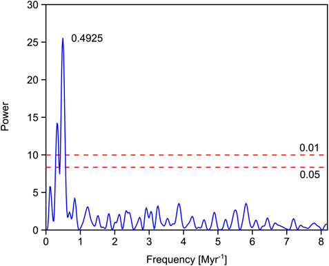
FIGURE 5. Simple periodogram for the bulk organic carbon isotope record from Pakistan. The peak with highest power depicting a ∼2 Myr cyclicity. The two red dashed lines represent the 0.01 and 0.05 significance levels.
Discussion
Regime Shifts
Despite the known shortcomings of paleontological records with respect to time resolution and data accuracy (taphonomic processes and taxonomic resolution) (DiMichele et al., 2009), deep-time records are valuable in order to unravel the interplay of biotic and abiotic factors creating or destroying resilience and thus the potential to absorb perturbations (Willis et al., 2010). One of the most stunning analyses of deep-time records with respect to possible existence of regime shifts concerns vegetation-climate interactions during the Middle-Late Pennsylvanian and the Pennsylvanian–Permian transitions (DiMichele et al., 2009). The possibility of the existence of alternative regimes in tropical wetland vegetation during the middle–late Pennsylvanian has been conclusively demonstrated, whereas the vegetation response to climate change at the Pennsylvanian–Permian boundary shows a non-hysteretic threshold response (DiMichele et al., 2009).
For the Early Triassic palynofloral record from Pakistan, the results of the exploratory analysis reveal some abrupt shifts e.g. in first principle component, whereas isotope trends seem to be more gradual (Figure 4). Changes in carbon isotope records reflect changes in carbon cycling, and are regarded to reflect environmental changes (Payne et al., 2004; Weissert, 2019). Oxygen isotope data from conodont apatite can be used to reconstruct sea temperatures (e.g. Romano et al., 2013; Trotter et al., 2015; Goudemand et al., 2019). Thus, there are two proxy records for Early Triassic environmental changes: bulk organic carbon isotopes and conodont apatite oxygen isotopes. The most remarkable interval spans the late early Smithian to the early Spathian and is discussed first for the possible presence of thresholds with or without hysteresis.
During the late early Smithian, bulk organic carbon isotope values start to decrease, whereas sea temperatures start to rise (Hermann et al., 2011b; Romano et al., 2013), these changes are not accompanied by gradual changes in vegetation composition. In contrast, the vegetation reacted only late to these trends, but then abruptly (PC1, PC2, dominance, spore/pollen ratios). Such ecosystem behavior reflects a threshold response to gradual/incremental environmental changes (e.g. Anderson et al., 2009). The vegetation is tipping from a mixed early Smithian lycophyte-gymnosperm vegetation to a lycophyte dominated vegetation in the middle Smithian. Diversity seems to dwindle synchronously with the changing environmental proxies, whereas dominance and both principle components show threshold responses. The shift in dominance from low values in the early Smithian to high values in the middle Smithian indicates that the middle Smithian vegetation was dominated by only a few plant taxa, whereas during the early Smithian taxa were rather equally present.
Both abiotic proxies (δ18O and δ13C) start to rise again during the middle Smithian. A sharp shift to gymnosperm-dominated vegetation (documented also in both principle components and a drop in dominance) occurs at the middle–late Smithian boundary co-occurring with δ18O and δ13C values both higher than those at the early–middle Smithian transition. The shift to gymnosperm-dominated vegetation seems to occur at a switch point (switch point 2 in Figure 1) with different environmental conditions compared to switchpoint 1. Thus, a threshold response with hysteresis is likely (Scheffer et al., 2001; Anderson et al., 2009).
The Griesbachian to Dienerian transition is difficult to interpret as the Griesbachian is surely underrepresented in the Pakistani records. The Griesbachian appears to be a transition phase between gymnosperm-dominated Permian plant communities and lycophyte-dominated Dienerian communities. Thus, indicating generally no abrupt change at the Permian-Triassic or Griesbachian-Dienerian boundary in the successions of Pakistan. Nevertheless, the contrast in plant composition, diversity, dominance, principle components between the Permian and the Dienerian is striking. Therefore, information from other regions are discussed here, in order to unravel changes in vegetation between the Permian and the Dienerian in greater detail, which are blurred by low resolution in Pakistan. Nearby successions (Australia, Madagascar) would be ideal for a comparison, however, they have partly a similar resolution (Balme, 1963) or have shortcomings with respect to independent age control (Goubin, 1965; Dolby and Balme 1976). Thus, the Kap Stosch successions in Greenland with high sampling resolution offers the opportunity to zoom into the upper part of the blurred interval in Pakistan, the Griesbachian–Dienerian transition interval. There, palynological records reveal that the Permian and the Griesbachian vegetation was dominated by gymnosperms. The main vegetation shift from gymnosperm-dominated to lycophyte-dominated vegetation occurred close to the Griesbachian–Dienerian boundary (Hochuli et al., 2016). However, while this succession was situated on a comparable latitude in the Northern Hemisphere, it might have been exposed to different environmental/climatic conditions (e.g. Kutzbach and Ziegler, 1993). A direct comparison is therefore implausible and not intended. However, looking beyond the southern subtropics illustrates that other ecosystems were affected by environmental changes and show abrupt reactions during the Griesbachian–Dienerian transition, although these might not be comparably obvious in the Pakistan records due to low resolution in the Griesbachian. Oxygen isotopes from Pakistan indicate that sea temperature started to increase at the Griesbachian–Dienerian boundary (Romano et al., 2013), whereas the Kap Stosch bulk organic carbon isotope record is marked by a negative shift across this boundary (Sanson-Barrera et al., 2015). The changes in vegetation composition occurs during the negative shift, thus, the changes in Greenland might well be a threshold response to environmental changes.
After highlighting environmental and vegetation changes in the upper boundary of the Griesbachian, which is not well resolved in the Pakistani records, we turn now to its older part, the Permian–Triassic boundary. As for the Griesbachian–Dienerian boundary, Northern Hemisphere sedimentary archives offer an exquisite view on the microfloral changes around the Permian–Triassic boundary. These reveal another shift from gymnosperm-dominated to lycophyte-dominated vegetation in Jameson Land (Greenland) and Finnmark (Norway) data sets (Looy et al., 2001; Hochuli et al., 2010a). These coincide with the negative carbon isotope shift that marks the Permian–Triassic boundary in this succession and worldwide (Korte and Kozur, 2010). Gymnosperms recovered relatively quickly and dominate Griesbachian assemblages (Hochuli et al., 2010a). The resolution of environmental proxies is limited but the position of the vegetation shift within the negative carbon isotope excursion might indicate threshold response. In the Pakistan records, this specific shift close to the Permian–Triassic boundary is not resolved. At Narmia,∼10 km East of Chitta-Landu, two samples from below the Kathwai Member are marked by high lycophyte spore abundances, however, these occurrences are too few and are stratigraphically isolated and cannot be correlated with the so-called spore peak from the Northern Hemisphere succession. However, palynological and bulk organic carbon isotope data are available from the Denison NS 20 borehole from the Australian Bowen Basin. There, the Protohaploxypinus microcorpus Zone is marked by high lycophyte spore abundances of up to 80% (Foster, 1982), thus, reaching similar spore abundances as during the spore peak in the Finnmark record (Hochuli et al., 2010a). This zone of high lycophyte spore abundance in the Australian Denison NS 20 borehole occurs within the negative carbon isotope shift (Morante, 1996), like the one in the Northern Hemisphere. Thus, the shift from gymnosperm-dominated vegetation to lycophyte-dominated vegetation is therefore not only recorded from the Northern Hemisphere, but also from the Southern Hemisphere. A shift back to gymnosperms as in the Northern Hemisphere is not recorded. However, Southern Hemisphere records show distinct regional patterns, e.g. in Antarctica palynofloras are marked by an increase in diversity throughout the supposed boundary interval (Lindström and McLoughlin, 2007). Whereas in east Australia, even records from the same basin (Sydney Basin) show different palynofloral development prior to the Permian–Triassic transition. The interval containing the youngest Permian coal deposits has attracted high attention. In the northeastern part of the Sydney Basin, a marked shift from gymnosperm dominance to higher spore abundances with many taxa “surviving” the deposition of the youngest coal is documented (Grebe, 1970) whereas continued spore dominance throughout the same stratigraphic interval is known from the central part of the Sydney Basin (Mays et al., 2020), There, specific fern spores (Thymospora) dominate palynological assemblages soon after the deposition of the uppermost Permian coal, indicating significant changes in vegetation composition prior to the above mentioned shift from gymnosperm-dominance to lycophyte-dominance associated with the carbon isotope negative shift. Therefore, local climatic effects and differences in depositional environments can influence palaeobotanical records dramatically and aggravate their comparability. In summary, the time interval from the Permian–Triassic boundary up to the Smithian–Spathian boundary is a time with several major regime shifts, but they are not recorded everywhere.
Focusing on the time interval after the middle–late Smithian events, the Spathian interval is generally marked by a mixed gymnosperm-lycophyte vegetation. An interval approximately in the middle of the Spathian shows increased dominance and reduced diversity together with a higher contribution of lycophytes in the palynological assemblages. These changes are reflected only to a limited extend in PC 1, and are not obvious in PC 2, but coincide with a minor negative carbon isotope excursion. Stabilization of the environmental and ecological situations during the Spathian has been also reported from the boreal realm (Galfetti et al., 2007b; Hochuli and Vigran, 2010; Lindström et al., 2019), South China (Saito et al., 2013). In the marine realm, ecosystems also seem to stabilize (e.g. Brayard et al., 2006) or start to increase continuously in diversity during the Spathian (e.g. Hofmann et al., 2014).
For the Early Triassic subtropical paleoecological archive of Pakistan, two prominent regimes stand out, one gymnosperm-dominated regime seemingly coinciding with cooler conditions and the lycophyte-dominated regime thriving predominantly under warmer conditions. Thus, plant communities seem to bounce between two regimes. However, the picture is complicated by transient vegetation types during the early Smithian and Spathian, which will be discussed later. First, possible positive feedbacks for each regime are addressed. Positive feedbacks are regarded essential for the facilitation and stabilization of alternative regimes. However, their existence alone cannot be regarded as ultimate proof for the presence of alternative regimes but positive feedback can strongly support the argumentation for alternative regimes in combination with other approaches (Scheffer et al., 2001; Scheffer and Carpenter, 2003).
Stabilizing Factors of Each Regime
Prominent representatives of Early Triassic lycophytes include Isoetes and Pleuromeia (Retallack, 1997). Pleuromeia can even be regarded as the iconic plant of the Early Triassic that occurred almost worldwide (Krassilov and Karasev, 2009). Pleuromeiales are represented in the Pakistani records by the dispersed spore genera Aratrisporites., Lundbladispora, and Densoisporites (Balme, 1995). Roots of these lycophytes were composed of rhizospheres or corms with rootlets extending from it. With their rather simple rooting systems, they were adapted to unstabilized soil, and able to grow in waterlogged disturbed ecosystems (Retallack, 1975; Retallack, 1997; Feng et al., 2020) such as in riparian ecosystems (Kustatscher et al., 2014). Plant associations are sensitive to climatic changes not only under the modern global change (e.g. Bjorkman et al., 2018) but also past plant associations were influenced by climatic conditions (e.g. Birks et al., 2016).
Pakistan was situated geographically in the southern subtropics exposed to the climatic conditions of the monsoon system with the intertropical convergence zone responsible for a high seasonality in precipitation and temperature (Kutzbach and Gallimore, 1989; Kutzbach and Ziegler, 1993; Parrish, 1993; Rees et al., 1999; Gibbs et al., 2002; Roscher et al., 2011). Changes in insolation seasonality have been modeled to influence monsoon strength (Kutzbach, 1994). Increased insolation seasonality induces increased strength of the monsoon circulation, i.e. an increase in precipitation seasonality and this increase leads to higher seasonal runoff (Kutzbach, 1994). Changes in the hydrological cycle influence weathering and sedimentation style and may lead to increased areas with unconsolidated soil in lowland areas. For the northern part of the Bowen Basin, a change from meandering rivers to a braided river system with unconstrained channels is documented to occur from the Permian Rangal Coal Measures to the Triassic Sagittarius Sandstone (Michaelsen, 2002). The rooting systems of lycophytes are incapable of stabilizing these soils creating a positive feedback of habitat instability and lycophyte cover.
The alternative regime is dominated by gymnosperms (mainly conifers and seed ferns) represented primarily in the palynological assemblages of Pakistan by bisaccate pollen. Compared to lycophytes, these plants have diverse and partly complex rooting systems providing anchorage for long-term support of the plants, under less disturbed conditions. Moreover, complex rooting systems can contribute to stabilize unconsolidated soil (e.g. Micovski et al., 2009). The canopy of a gymnosperm-dominated vegetation was rather closed, therefore, reducing the splash of rainfall and soil erosion compared to the more open canopy of a vegetation dominated by unbranched lycophytes (DiMichele et al., 2009; Taylor et al., 2009). Additionally, the positive feedback of vegetation on precipitation is enhanced in forests compared to open vegetation. Thus, a higher transpiration in forests compared to lycophyte stands dominated by Pleuromeiales fosters the local recycling of moisture and thus can plausibly provoke rainfall during dry seasons, analogous to the alternative regimes (forest vs savannah) in the modern Amazon region (Scheffer, 2009). However, research on functional trait changes through time is a developing field, the contrast in conductive capacity between Pleuromeiales and gymnosperms might be less significant for the vegetation-climate feedback (Wilson et al., 2017).
Thus, changes in the climate system that cause variations in insolation, temperature contrast and thus monsoon intensity together with feedback mechanisms, could determine which regime is dominant at any particular time between the Permian–Triassic and the middle–late Smithian boundaries.
Why During the Early Triassic? What Caused the Resilience to Diminish?
The Permian–Triassic transition is remarkable, not only because the biggest mass extinction in Earth history is associated with this time interval, it also marks a milestone in global phytogeographic development. The four distinct and isolated Late Permian floral kingdoms (Cathaysia, Angara, Gondwana, Euramerica) declined and a new northern Laurussian and a southern Gondwana kingdom formed. The Early Triassic is regarded a key interval in this transitions, in which Pleuromeiales show temporary cosmopolitan distribution (Dobruskina, 1987; Karasev and Krassilov, 2009). Thereafter, phytogeographic kingdom boundaries were roughly latitudinally aligned. Since then, the main phytogeographical zonation has not changed much (Dobruskina 1987, 1995). The Early Triassic vegetation changes in the southern subtropics of Pakistan occurred within the context of this major global phytogeographic reorganization.
While searching for a possible trigger for the ecological events starting at the Permian–Triassic transition and continuing up to the middle–late Smithian, the focus is drawn to the timing of these events. The first large scale abrupt regime shifts associated with a carbon isotope negative shift are documented from Permian–Triassic boundary successions in Australia, gymnosperm-dominated Permian vegetation is replaced by a lycophyte-dominated one (Foster, 1982) in the Bowen Basin. However, the timing of the vegetation response to environmental changes around the Permian–Triassic transition might be even more complex (Fielding et al., 2019). In Norway and Greenland, gymnosperm dominated vegetation is restored quickly, thus the preceding interval is referred to as a spore peak (Looy et al., 2001; Hochuli et al., 2010b). For the Sydney Basin, a fern spore peak soon after the decline of Glossopterids is present, as well as a late shift to pleuromeians in the Smithian (Mays et al., 2020). Similar events occur ∼2.4 Myrs later, during middle–late Spathian times as documented in the Pakistan successions, again in association with a negative carbon isotope shift. Thus, the two events are separated by a time interval of ∼2.4 Myrs. To talk of periodicities with only two events documented in a row is admittedly boldfaced. Especially, if the older event is most probably associated with the environmental perturbations causing the Permian–Triassic mass extinction. However, in the search for a possible cause of the subsequent Early Triassic vegetation pattern, one option could be orbital climate forcing. Periodicities of this length are known to occur in Earth’s orbit eccentricity as long-term cycles (Laskar et al., 2011).
The influence of long-term eccentricity periods on carbon cycling have been documented for the Thracian Oceanic Anoxic Event and Cenozoic successions (Pälike et al., 2006; Boulila et al., 2012; Boulila et al., 2014). However, these are marked by shorter cyclicity (1.6 Myr) supporting the instability of the length of this period indicated by astronomical modeling (∼2 Myr for the Thracian and ∼2.4 Myr for the Boulila et al., 2014). The simple periodogram for the bulk organic carbon isotope record from Pakistan (Figure 5), reveals a periodicity of ∼2.03 Myr, which lies within the range of astronomically predicted periodicities for this term. However, it is shorter than the stratigraphically deduced period length of ∼2.4 Myr. A close correspondence between carbon isotope excursions and climatic upheavals and the long-term eccentricity periodicity has been also documented for the Paleocene–Eocene boundary event (Lourens et al., 2005). Thus, these periodicities are documented in sedimentary archives and are known to cause climatic shifts (Kump et al., 2005; Scheffer, 2009). The Pakistani records are marked by uneven sampling density and the lack of appropriate samples for radiometric dating, therefore, uncertainties with respect to periodicities are inevitable. Pakistan during the Early Triassic was exposed to the peculiar circulation pattern of a large monsoon system, driven by large landmasses in the mid-to low latitudes and the tropical Tethys ocean. One key factor that could trigger changes in monsoon intensity is orbital forcing. Precession and eccentricity determine the duration and geographic position of insulation maxima and thus the intensity of the monsoon (Mohtadi et al., 2016). For Pangea, an increase in monsoon intensity and thus increase in summer rainfall and runoff have been simulated to occur in the hemisphere with summer solstice occurring at perihelion (Kutzbach, 1994). Thus, changes in insolation by orbital forcing causes higher seasonality in precipitation and could work in concert with positive feedback mechanisms to trigger ecosystem regime shifts. A similar combined mechanism has been proposed for sharp shifts in the Pleistocene climate system (Scheffer, 2009). For the Early an increase in Southern Hemisphere seasonality in precipitation and temperature contrasts in the Northern Hemisphere with decreased seasonality (Kutzbach, 1994). Thus, climatic conditions are changing as well but less pronounced. However, the discussion on orbital climate forcing potential during the Early Triassic would profit from climate reconstructions based on more comprehensive models as recently used for the Permian (Kiehl and Shields, 2005; Montenegro et al., 2011). The Smithian–Spathian boundary interval has been documented from northern Greenland and the Barents Sea areas (Galfetti et al., 2007b; Lindström et al., 2019). Both localities show dominance of spores in the Smithian and pollen dominated assemblages in the Spathian. The shift occurs near the Wasatchites tardus ammonoid zone, which corresponds to the basal ammonoid zone of the late Smithian in Pakistan. Exact correlation of the events in Pakistan with the Northern Hemisphere is hampered because of a supposed sedimentary gap in the northern successions encompassing most of the late Smithian (Hammer et al., 2019). However, both critical time intervals, the Permian–Triassic as well as the Smithian–Spathian boundary intervals are associated with changes in the palynofloral records in both hemispheres.
If the timing of vegetation changes around the middle–late Smithian fit into the orbitally paced scheme, then what about the Dienerian? Relative abundance of lycophyte spores, generic diversity and to certain amount PC1 are comparable to the middle Smithian values. In the high resolution succession from Greenland, the drastic shift is even more discrete from the Griesbachian to the Dienerian. According to the depth-age model, the Griesbachian accounts for 400 ka (note that in Figure 4, the boundary is biostratigraphically adjusted, and radiometric dating is not available) which roughly corresponds to the 405 years term in eccentricity (Laskar et al., 2011). Keep in mind that the Greenland vegetation was exposed to different climatic conditions compared to Pakistan. While Pakistan was facing the Tethyan coast and thus prone to receive summer rainfall, Greenland had an averted position with respect to the tropical Tethys (Kutzbach and Gallimore, 1989). The regional ecosystem might have had its own peculiarities/vulnerabilities concerning orbital climate forcing.
However, orbital forcing was operating before and after the Early Triassic, seemingly with little impact on plant associations then. Contrastingly, Early Triassic terrestrial ecosystems seem to have been particularly susceptible to these orbitally forced climate changes. Turning to the dynamical landscape of alternative regimes, resilience has been described as the altitudinal difference between valleys and separating heights. If a system is manipulated in a way that the resilience is reduced, minor additional perturbations or stochastic events can cause regime shifts (Scheffer et al., 2001).
In present-day ecosystems a loss in resilience is induced by biodiversity loss, introduction of pollutants, climate change, and/or regional destruction of standing biomass (Peterson et al., 1998; Folke et al., 2004; Zemp et al., 2017). Environmental changes such as introduction of pollutants or climate change are regarded as fundamental effects influencing ecosystems by reducing (functional) biodiversity. A loss in functional-group diversity has a great impact on the performance of an ecosystem, e.g. the loss of functional groups might destroy trophic networks or open up niches for invasive species (Folke et al., 2004) The same suite of disturbances have been revealed and documented for the Permian–Triassic boundary.
A large igneous province, the Siberian Traps, not only CO2 into the atmosphere causing climatic upheavals, but also halocarbons (Svensen et al., 2009; Black et al., 2012), mercury (Sanei et al., 2012), and other aerosols (Grasby et al., 2011). The main volcanic phase occurred within less than one million years straddling the Permian–Triassic boundary (Burgess & Bowring, 2015), however, magmatic activity continued into the Early Triassic (Augland et al., 2019) (Figure 4). The environmental changes were profound and caused the loss of oceanic faunal diversity (e.g., Raup and Sepkoski, 1982). How severe the continental fauna was affected is still discussed (Benton et al., 2004; Lucas, 2009). Thus, the Earth system was hit hard and was no longer able to absorb additional small scale perturbations. Or, to stay in the metaphorical picture of a landscape, the altitudinal differences of the dynamical landscape were reduced, mountains were eroded, valleys and basins filled, resilience was a victim of this erosion. Therefore, after the initial strike of the Permian–Triassic events, southern subtropical ecosystems were vulnerable toward small scale perturbations such as orbitally forced climate changes that could push ecosystems in almost any direction.
Because of the low relief of the dynamical landscape, the expressed lycophyte or gymnosperm regime (state, valley or basin) might not always be the most probable state the ecosystem is compelled to. The early Smithian palynomorph assemblages show transient characters; this behavior could be described as transient ecosystem behavior (e.g. Hastings et al., 2018). Moving on the dynamical landscape toward one of the valleys, but being retarded or detoured by a so-called ghost attractor (e.g. a basin has been filled and therefore offers no longer a stable state, the ecosystem lingers around instead of moving immediately to the next stable state) or exhibits a crawl-by behavior (the ecosystem is attracted by a stable basin, however a saddle blocks the direct way causing a detour along the saddle) (Hastings et al., 2018). Transient behaviors in ecosystems can persist for a long time leading to abrupt shifts in ecosystems without significant environmental changes (Hastings et al., 2018).
After the middle–late Smithian regime shifts, a mixed lycophyte-gymnosperm vegetation prevailed. Additionally, some palynofloral components changed in relative abundances compared to the lower part of the Lower Triassic (Aratrisporites vs. Lundbladispora; non-taeniate bisaccate pollen vs. taeniate bisaccate pollen). Environmental perturbations, as indicated by the negative carbon isotope negative shift in the intermittent interval within the Spathian, had only limited influence and did not cause a dramatic shift. The Spathian vegetation was seemingly better buffered, and on track in restoring resilience. The importance of maintaining resilience can be for the persistence of an ecosystem has been documented for littoral forests in Madagascar. In the face of late Holocene environmental changes, the onlypatches of forests that recovered were those able to restore their taxonomic richness due to a higher resilience, other areas transformed into permanent heathland (Virah-Sawmy et al., 2009). Biodiversity is regarded as a fundamental factor for ecosystem resilience (Folke et al., 2004). The generic richness of the studied succession shows reduced diversity during the Dienerian and during the middle and late Smithian in Pakistan, corresponding to those intervals in which the results of the exploratory analysis suggest the occurrence of regime shifts (Figure 4). Recovery trends of diversity are observed in the early Smithian, early Spathian and late Spathian–Anisian. Thus, changes in biodiversity might be a signal for resilience of local ecosystems in deep-time records. However, taphonomic biases must be considered, and the sudden disappearance of fossils and thus diversity might be of local significance only.
Southern subtropical Early Triassic terrestrial ecosystems were fragile due to the Permian–Triassic events; therefore, the drastic regime shifts reflect the sensibility of the system to forcing mechanisms. Before and thereafter, resilience was high and ecosystems buffered the effects of orbital forcing.
Conclusion
The Early Triassic vegetation patterns are complex and their underlying determinants far from being understood. Instead of focusing on repeated volcanically induced deteriorations, here the palynological records from Pakistan (together with Northern Hemisphere records) are discussed under the premise of the alternative stable state theory. The Permian–Triassic, the Griesbachian–Dienerian, and the middle–late Smithian boundary stand out with abrupt shifts between lycophyte-dominated vegetation and gymnosperm-dominated vegetation. However, proving the existence of alternative stable regimes in deep-time records is difficult. Exploratory data analysis indicates that threshold response is likely in all cases, and hysteresis is plausible for the abrupt shifts occurring during the middle and late Smithian. Ecosystems with low resilience are prone to regime shifts that can be triggered by small perturbations. The Pakistani palynoforal record indicates that vegetation in the first half of the Early Triassic was sensitive to environmental disturbance. The timing of the major events (middle–late Smithian∼2.4 Myrs, Dienerian ∼400 kyrs after the Permian–Triassic biotic and abiotic events), possibly indicates orbital-forcing responsible for these changes. However, orbitally forced regime shifts in vegetation have not be recorded directly before and after the Early Triassic. Working together, phytochoria reorganization and the profound environmental and biotic changes of the Permian–Triassic events reduced resilience and increased susceptibility to minor environmental/climatic changes.
The alternative considerations presented will hopefully encourage further research into whether the loss of resilience, aside from taphonomic and paleogeographic controls, could be a cause for the differing regional s of vegetation response to the Permian–Triassic boundary events documented in the fossil record. The discussion whether there had been a global plant mass extinction or not is continuing. Plants probably did not become extinct on a large scale, but their distribution in space and time was fluctuating enormously due to environmental changes, but also probably because of lowered resilience, and therefore extreme shifts in composition, creating the impression of virtual absence. There might be more than one possible explanation for temporal variations in complex ecosystems.
Data Availability Statement
Data for this study are available in the Dryad Digital Repository: https://doi.org/10.5061/dryad.r4xgxd29v
Author Contributions
ES-H designed the study, analyzed the data, and wrote the manuscript.
Funding
Basic palynological, biostratigraphical, and carbon isotope data were based on Swiss National Science Foundation projects PBZHP2-135955 (to ES-H) and 200020-127716/1 (to H. Bucher).
Conflict of Interest
The author declares that the research was conducted in the absence of any commercial or financial relationships that could be constructed as a potential conflict of interest.
The handling editor declared a past co-authorship with the author (ES-H).
Acknowledgments
For years of discussion, support and company during field campaigns I am indebted to Peter A. Hochuli†, Hugo Bucher, Thomas Brühwiler, David Ware, Nicolas Goudemand, Michael Hautmann, Ghazala Roohi and the entire team of the National History Museum of Pakistan in Islamabad. I thank Barry Lomax and Chris Mays for their constructive comments on this manuscript. Figures were created using Inkscape 0.92.4.
References
Algeo, T. J., Brayard, A., and Richoz, S. (2019). The Smithian-Spathian boundary: a critical juncture in the Early Triassic recovery of marine ecosystems. Earth Sci. Rev. 195, 1–6. doi:10.1016/j.earscirev.2019.102877.
Andersen, T., Carstensen, J., Hernández-García, E., and Duarte, C. M. (2009). Ecological thresholds and regime shifts: approaches to identification. Trends Ecol. Evol. 24 (1), 49–57. doi:10.1016/j.tree.2008.07.014.
Augland, L. E., Ryabov, V. V., Vernikovsky, V. A., Planke, S., Polozov, A. G., Callegaro, S., et al. (2019). The main pulse of the Siberian Traps expanded in size and composition. Sci. Rep. 9 (1), 1–12. doi:10.1038/s41598-019-54023-2.
Balme, B. E. (1995). Fossil in situ spores and pollen grains: an annotated catalogue. Rev. Palaeobot. Palynol. 87, 81–323. doi:10.1016/0034-6667(95)93235-x.
Balme, B. E. (1963). Plant microfossils from the lower triassic of western Australia. Palaeontology 6 (1), 12–40.
Becker, L., Poreda, R. J., Basu, A. R., Pope, K. O., Harrison, T. M., Nicolson, C., and Iasky, R. (2004). Bedout: a possible end-permian impact crater offshore of northwestern Australia. Science 304, 1469–1476. doi:10.1126/science.1093925.
Benton, M. J.,, and Newell, A. J. (2014). Impacts of global warming on Permo-Triassic terrestrial ecosystems. Gondwana Res. 25, 1308–1337. doi:10.1016/j.gr.2012.12.010.
Benton, M. J., Tverdokhlebov, V. P., and Surkov, M. V. (2004). Ecosystem remodelling among vertebrates at the Permian-Triassic boundary in Russia. Nature 432, 97–100. doi:10.1038/nature02950.
Birks, H. J. B., Birks, H. H., and Ammann, B. (2016). The fourth dimension of vegetation. Science 354, 412–413. doi:10.1126/science.aai8737.
Bjorkman, A. D., Myers-Smith, I. H., Elmendorf, S. C., Normand, S., Rüger, N., Beck, P. S. A., et al. (2018). Plant functional trait change across a warming tundra biome. Nature 562 (7725), 57–62. doi:10.1038/s41586-018-0563-7.
Black, B. A., Elkins-Tanton, L. T., Rowe, M. C., and Peate, I. U. (2012). Magnitude and consequences of volatile release from the Siberian Traps. Earth Planet Sci. Lett. 317-318 (318), 363–373. doi:10.1016/j.epsl.2011.12.001.
Bomfleur, B., Decombeix, A. L., Escapa, I. H., Schwendemann, A. B., and Axsmith, B. (2013). Whole-plant concept and environment reconstruction of a Telemachus conifer (voltziales) from the triassic of Antarctica. Int. J. of Plant Sci., 174 (3), 425–444. doi:10.1086/668686.
Boulila, S., Galbrun, B., Huret, E., Hinnov, L. A., Rouget, I., Gardin, S., and Bartolini, A. (2014). Astronomical calibration of the Thracian Stage: implications for sequence stratigraphy and duration of the early Thracian OAE. Earth Planet Sci. Lett. 386, 98–111. doi:10.1016/j.epsl.2013.10.047.
Boulila, S., Galbrun, B., Laskar, J., and Pälike, H. (2012). A ∼9myr cycle in Cenozoic δ13C record and long-term orbital eccentricity modulation: is there a link?. Earth Planet Sci. Lett. 317-318 (318), 273–281. doi:10.1016/j.epsl.2011.11.017.
Brayard, A., Bucher, H., Escarguel, G., Fluteau, F., Bourquin, S., and Galfetti, T. (2006). The Early Triassic ammonoid recovery: paleoclimatic significance of diversity gradients. Palaeogeogr. Palaeoclimatol. Palaeoecol. 239, 374–395. doi:10.1016/j.palaeo.2006.02.003.
Brayard, A., Escarguel, G., and Bucher, H. (2005). Latitudinal gradient of taxonomic richness: combined outcome of temperature and geographic mid-domains effects?. J Zoological System. 43 (3), 178–188. doi:10.1111/j.1439-0469.2005.00311.x.
Brayard, A., Escarguel, G., Bucher, H., Monnet, C., Brühwiler, T., Goudemand, N., et al. (2009). Good genes and good luck: ammonoid diversity and the end-permian mass extinction. Science 325, 1118–1121. doi:10.1126/science.1174638.
Brosse, M., Bucher, H., and Goudemand, N. (2016). Quantitative biochronology of the Permian-Triassic boundary in South China based on conodont unitary associations. Earth Sci. Rev. 155, 153–171. doi:10.1016/j.earscirev.2016.02.003.
Brühwiler, T. (2010). Smithian (Early Triassic) ammonoid faunas of the Tethys: taxonomy, biochronology, diversity dynamics and palaeoenvironments. Mathematisch-naturwissenschaftliche Fakultät, Universität Zürich, Zürich, 673.
Burgess, S. D.,, and Bowring, S. A. (2015). High-precision geochronology confirms voluminous magmatism before, during, and after Earth’s most severe extinction. Sci. Adv. 1 (7), e1500470. doi:10.1126/sciadv.1500470.
Burgess, S. D., Bowring, S., and Shen, S.-z. (2014). High-precision timeline for Earth's most severe extinction. Proc. Natl. Acad. Sci. USA. 111, 3316–3321. doi:10.1073/pnas.1317692111.
Cascales-Miñana, B., Diez, J. B., Gerrienne, P., and Cleal, C. J. (2016). A palaeobotanical perspective on the great end-Permian biotic crisis. Hist. Biol. 28 (8), 1066–1074. doi:10.1080/08912963.2015.1103237.
Chu, D., Grasby, S. E., Song, H., Corso, J. D., Wang, Y., Mather, T. A., et al. (2020). Ecological disturbance in tropical playlands prior to marine Permian-Triassic mass extinction. Geology 48, 288–292. doi:10.1130/G46631.1
DiMichele, W. A., Montañez, I. P., Poulsen, C. J., and Tabor, N. J. (2009). Climate and vegetational regime shifts in the late Paleozoic ice age earth. Geobiology 7, 200–226. doi:10.1111/j.1472-4669.2009.00192.x.
Dobruskina, I. A. (1987). Phytogeography of Eurasia during the early triassic. Palaeogeogr. Palaeoclimatol. Palaeoecol. 58 (1–2), 75–86. doi:10.1016/0031-0182(87)90007-1.
Dolby, J. H.,, and Balme, B. E. (1976). Triassic palynology of the carnarvon basin, western Australia. Rev. Palaeobot. Palynol. 22, 105–168. doi:10.1016/0034-6667(76)90053-1.
Feng, Z., Wei, H. B., Guo, Y., He, X. Y., Sui, Q., Zhou, Y., et al. (2020). From rainforest to herbland: new insights into land plant responses to the end-Permian mass extinction. Earth Sci. Rev. 204, 103153. doi:10.1016/j.earscirev.2020.103153.
Fielding, C. R., Frank, T. D., Mcloughlin, S., Vajda, V., Mays, C., Tevyaw, A. P., et al. (2019). Age and pattern of the southern high-latitude continental end-Permian extinction constrained by multiproxy analysis. Nat. Commun., 10, 385–412. doi:10.1038/s41467-018-07934-z.
Folke, C., Carpenter, S., Walker, B., Scheffer, M., Elmqvist, T., Gunderson, L., et al. (2004). Regime shifts, resilience, and biodiversity in ecosystem management. Annu. Rev. Ecol. Evol. Syst. 35, 557–581. doi:10.1146/annurev.ecolsys.35.021103.105711.
Foster, C. B. (1982). Spore-pollen assemblages of the Bowen Basin, queensland (Australia): their relationship to the permian/triassic boundary. Rev. Palaeobot. Palynol. 36, 165–183. doi:10.1016/0034-6667(82)90016-1.
Fraiser, M. L., and Bottjer, D. J. (2005). Restructuring in benthic level-bottom shallow marine communities due to prolonged environmental stress following the end-Permian mass extinction. Comptes Rendus Palevol. 4, 583–591. doi:10.1016/j.crpv.2005.02.002.
Fuchs, G., Grauvogel-Stamm, L., and Mader, D. (1991). Une remarquable flore à Pleuromeia et Anomopteris in situ du Bundsandstein moyen (Trias inférieur) de L’Eifel (R.F. Allemagne) morphologie, Paléoécologie et aPaléogéographie. Palaeontographica Abteilung B, 222, 89–120.
Galfetti, T., Bucher, H., Ovtcharova, M., Schaltegger, U., Brayard, A., Brühwiler, T., et al. (2007a). Timing of the Early Triassic carbon cycle perturbations inferred from new U-Pb ages and ammonoid biochronozones. Earth Planet Sci. Lett. 258, 593–604. doi:10.1016/j.epsl.2007.04.023.
Galfetti, T., Hochuli, P. A., Brayard, A., Bucher, H., Weissert, H., and Vigran, J. O. (2007b). Smithian-Spathian boundary event: evidence for global climatic change in the wake of the end-Permian biotic crisis. Geol. 35 (4), 291–294. doi:10.1130/g23117a.1.
Gastaldo, R. A., Kamo, S. L., Neveling, J., Geissman, J. W., Bamford, M., and Looy, C. V. (2015). Is the vertebrate-defined Permian-Triassic boundary in the Karoo Basin, South Africa, the terrestrial expression of the end-Permian marine event?. Geology 43, 939–942. doi:10.1130/g37040.1.
Gastaldo, R. A., Kamo, S. L., Neveling, J., Geissman, J. W., Looy, C. V., and Martini, A. M. (2020). The base of the Lystrosaurus Assemblage Zone, Karoo Basin, predates the end-Permian marine extinction. Nat. Commun. 11 (1), 1–8. doi:10.1038/s41467-020-15243-7.
Gibbs, M. T., Rees, P. M., Kutzbach, J. E., Ziegler, A. M., Behling, P. J., and Rowley, D. B. (2002). Simulations of permian climate and comparisons with climate‐sensitive sediments. J. Geol. 110, 33–55. doi:10.1086/324204.
Goubin, N. (1965). Description et Répartition des principaux pollenites Permiens, Triassiques et Jurassiques des sondages du bassin de Morondava (Madagascar). Revue de l’institute Francais Du Pétrole et Annales Des Combustibles Liquides. 20 (10), 1415–1461.
Goudemand, N., Romano, C., Leu, M., Bucher, H., Trotter, J. A., and Williams, I. S. (2019). Dynamic interplay between climate and marine biodiversity upheavals during the early Triassic Smithian -Spathian biotic crisis. Earth Sci. Rev. 195, 169–178. doi:10.1016/j.earscirev.2019.01.013
Goudemand, N. (2011). Taxonomy and biochronology of early triassic conodonts. Zürich, Switzerland: Mathematisch-naturwissenschaftliche FakultätUniversität Zürich, 193.
Grasby, S. E., Sanei, H., and Beauchamp, B. (2011). Catastrophic dispersion of coal fly ash into oceans during the latest Permian extinction. Nat. Geosci. 4, 104–107. doi:10.1038/ngeo1069.
Grebe, H. (1970). Permian plant microfossils from newcastle coal measures/narrabeen group boundary, lake munmoroah, new south wales. Record Geol. Surv. N. S. W. 12, 125–136.
Grice, K., Twitchett, R. J., Alexander, R., Foster, C. B., and Looy, C. (2005). A potential biomarker for the Permian-Triassic ecological crisis. Earth Planet Sci. Lett. 236, 315–321. doi:10.1016/j.epsl.2005.05.008.
Hammer, Ø., Harper, D. A. T., and Ryan, P. D. (2001). PAST: palaeontological statistics software package for education and data analysis. Palaeontol. Electron. 4 (4), 9pp.
Hammer, Ø., Jones, M. T., Schneebeli-Hermann, E., Hansen, B. B., and Bucher, H. (2019). Are Early Triassic extinction events associated with mercury anomalies? A reassessment of the Smithian/Spathian boundary extinction. Earth Sci. Rev. 195 (March), 179–190. doi:10.1016/j.earscirev.2019.04.016.
Hastings, A., Abbott, K. C., Cuddington, K., Francis, T., Gellner, G., Lai, Y. C., et al. (2018). Transient phenomena in ecology. Science 361 (6406), eaat6412. doi:10.1126/science.aat6412.
Hautmann, M., Bagherpour, B., Brosse, M., Frisk, Å., Hofmann, R., Baud, A., et al. (2015). Competition in slow motion: the unusual case of benthic marine communities in the wake of the end-Permian mass extinction. Palaeontology 58 (5), 871–901. doi:10.1111/pala.12186.
Hautmann, M., Bucher, H., Brühwiler, T., Goudemand, N., Kaim, A., and Nützel, A. (2011). An unusually diverse mollusc fauna from the earliest Triassic of South China and its implications for benthic recovery after the end-Permian biotic crisis. Geobios 44, 71–85. doi:10.1016/j.geobios.2010.07.004.
Hermann, E., Hochuli, P. A., Bucher, H., Brühwiler, T., Hautmann, M., Ware, D., and Roohi, G. (2011a). Terrestrial ecosystems on North Gondwana following the end-Permian mass extinction. Gondwana Res. 20, 630–637. doi:10.1016/j.gr.2011.01.008.
Hermann, E., Hochuli, P. A., Bucher, H., and Roohi, G. (2012). Uppermost permian to middle triassic palynology of the Salt range and surghar range, Pakistan. Rev. Palaeobot. Palynol. 169, 61–95. doi:10.1016/j.revpalbo.2011.10.004.
Hermann, E., Hochuli, P. A., Méhay, S., Bucher, H., Brühwiler, T., Ware, D., et al. (2011b). Organic matter and palaeoenvironmental signals during the early triassic biotic recovery: the Salt range and surghar range records. Sediment. Geol. 234 (1–4), 19–41. doi:10.1016/j.sedgeo.2010.11.003.
Heydari, E., Arzani, N., and Hassanzadeh, J. (2008). Mantle plume: the invisible serial killer - application to the Permian-Triassic boundary mass extinction. Palaeogeogr. Palaeoclimatol. Palaeoecol. 264, 147–162. doi:10.1016/j.palaeo.2008.04.013.
Hochuli, P. A., Hermann, E., Vigran, J. O., Bucher, H., and Weissert, H. (2010a). Rapid demise and recovery of plant ecosystems across the end-Permian extinction event. Global Planet. Change. 74 (3–4), 144–155. doi:10.1016/j.gloplacha.2010.10.004.
Hochuli, P. A., Sanson-Barrera, A., Schneebeli-Hermann, E., and Bucher, H. (2016). Severest crisis overlooked-Worst disruption of terrestrial environments postdates the Permian-Triassic mass extinction. Sci. Rep. 6, 28372. doi:10.1038/srep28372.
Hochuli, P. A.,, and Vigran, J. O. (2010). Climate variations in the boreal triassic - inferred from palynological records from the Barents Sea. Palaeogeogr. Palaeoclimatol. Palaeoecol. 290, 20–42. doi:10.1016/j.palaeo.2009.08.013.
Hochuli, P. A., Vigran, J. O., Hermann, E., and Bucher, H. (2010b). Multiple climatic changes around the Permian-Triassic boundary event revealed by an expanded palynological record from mid-Norway. Geol. Soc. Am. Bull. 122 (5–6), 884–896. doi:10.1130/b26551.1.
Hofmann, R., Hautmann, M., Brayard, A., Nützel, A., Bylund, K. G., Jenks, J. F., et al. (2014). Recovery of benthic marine communities from the end-Permian mass extinction at the low latitudes of eastern Panthalassa. Palaeontology 57, 547–589. doi:10.1111/pala.12076.
Holling, C. S. (1973). Resilience and stability of ecological systems. Annu. Rev. Ecol. Systemat. 4 (1), 1–23. doi:10.1146/annurev.es.04.110173.000245.
Holser, W. T., Schönlaub, H.-P., Attrep, M., Boeckelmann, K., Klein, P., Magaritz, M., et al. (1989). A unique geochemical record at the Permian/Triassic boundary. Nature 337, 39–44. doi:10.1038/337039a0.
Jablonski, D. (1986). Background and mass extinctions: the alternation of macroevolutionary regimes. Science 231 (4734), 129–133. doi:10.1126/science.231.4734.129.
Juggins, S. (2017). Rioja: analysis of quaternary science data, R package version. Available at: http://cran.r-project.org/package=rioja.0.9-21
Kidder, D. L.,, and Worsley, T. R. (2004). Causes and consequences of extreme Permo-Triassic warming to globally equable climate and relation to the Permo-Triassic extinction and recovery. Palaeogeogr. Palaeoclimatol. Palaeoecol. 203, 207–237. doi:10.1016/s0031-0182(03)00667-9.
Kiehl, J. T.,, and Shields, C. A. (2005). Climate simulation of the latest Permian: implications for mass extinction. Geol. 33 (9), 757. doi:10.1130/g21654.1.
Pakistani–Japanese Research Group (1985). “Permian and triassic systems in the Salt range and surghar range, Pakistan,” in The Tethys: her paleogeography and paleobiogeography from paleozoic to mesozoic. Editors K. Nakazawa, and J. M. Dickins (Tokyo, Japan: Tokai University Press), 221–312.
Knoll, A. H., Bambach, R. K., Canfield, D. E., and Grotzinger, J. P. (1996). Comparative earth history and late permian mass extinction. Science 273, 452–457. doi:10.1126/science.273.5274.452.
Korte, C.,, and Kozur, H. W. (2010). Carbon-isotope stratigraphy across the Permian-Triassic boundary: a review. J. Asian Earth Sci. 39, 215–235. doi:10.1016/j.jseaes.2010.01.005.
Krassilov, V.,, and Karasev, E. (2009). Paleofloristic evidence of climate change near and beyond the Permian-Triassic boundary. Palaeogeogr. Palaeoclimatol. Palaeoecol. 284, 326–336. doi:10.1016/j.palaeo.2009.10.012.
Kump, L. R., Pavlov, A., and Arthur, M. A. (2005). Massive release of hydrogen sulfide to the surface ocean and atmosphere during intervals of oceanic anoxia. Geol. 33 (5), 397–400. doi:10.1130/g21295.1.
Kustatscher, E., Franz, M., Heunisch, C., Reich, M., and Wappler, T. (2014). Floodplain habitats of braided river systems: depositional environment, flora and fauna of the Solling Formation (Buntsandstein, Lower Triassic) from Bremke and Fürstenberg (Germany). Palaeobiodivers. Palaeoenviron. 94 (2), 237–270. doi:10.1007/s12549-014-0161-0.
Kutzbach, J. E.,, and Gallimore, R. G. (1989). Pangaea climates: megamonsoons of the megacontinent. J. Geophys. Res. 94, 3341–3357. doi:10.1029/jd094id03p03341.
Kutzbach, J. E. (1994). “Idealized Pangea climates: sensitivity to orbital change.” in Geological Society of America Special Paper. Vol. 288, 41–56. doi:10.1130/spe288-p41.
Kutzbach, J. E.,, and Ziegler, A. M. (1993). Simulation of Late Permian climate and biomes with an atmosphere-ocean model: comparisons with observations. Philos. Trans. R. Soc. London, Ser. A B 341, 327–340.
Laskar, J., Fienga, A., Gastineau, M., and Manche, H. (2011). La2010: a new orbital solution for the long-term motion of the Earth. Astron. Astrophys. 532. doi:10.1051/0004-6361/201116836.
Lindström, S., Bjerager, M., Alsen, P., Sanei, H., and Bojesen-Koefoed, J. (2019). The Smithian–Spathian boundary in North Greenland: implications for extreme global climate changes. Geol. Mag. 157, 1547–1567. doi:10.1017/S0016756819000669
Lindström, S., McLoughlin, S., and Drinnan, A. N. (1997). Intraspecific variation of taeniate bisaccate pollen within permian glossopterid sporangia, from the prince charles mountains, Antarctica. Int. J. Plant Sci. 158 (5), 673–684. doi:10.1086/297479.
Lindström, S., and McLoughlin, S. (2007). Synchronous palynofloristic extinction and recovery after the end-Permian event in the Prince Charles Mountains, Antarctica: implications for palynofloristic turnover across Gondwana. Rev. Palaeobot. Palynol. 145, 89–122. doi:10.1016/j.revpalbo.2006.09.002.
Looy, C. V., Twitchett, R. J., Dilcher, D. L., van Konijnenburg-van Cittert, J. H. A., and Visscher, H. (2001). Life in the end-Permian dead zone. Proc. Natl. Acad. Sci. USA. 98 (14), 7879–7883. doi:10.1073/pnas.131218098.
Lourens, L. J., Sluijs, A., Kroon, D., Zachos, J. C., Thomas, E., Röhl, U., Bowles, J., and Raffi, I. (2005). Astronomical pacing of late Palaeocene to early Eocene global warming events. Nature 435, 1083–1087. doi:10.1038/nature03814.
Lucas, S. G. (2009). Timing and magnitude of tetrapod extinctions across the Permo-Triassic boundary. J. Asian Earth Sci. 36, 491–502. doi:10.1016/j.jseaes.2008.11.016.
Ludwig, D., Walker, B., and Holling, C. S. (1997). Sustainability, Stability, and Resilience. 1 (1), 1–19. doi:10.5751/es-00012-010107.
May, R. M. (1977). Thresholds and breakpoints in ecosystems with a multiplicity of stable states. Nature 269, 471–477. doi:10.1038/269471a0.
Mays, C., Vajda, V., Frank, T. D., Fielding, C. R., Nicoll, R. S., Tevyaw, A. P., and McLoughlin, S. (2020). Refined Permian-Triassic floristic timeline reveals early collapse and delayed recovery of south polar terrestrial ecosystems. Bull. Geol. Soc. Am. 132 (7–8), 1489–1513. doi:10.1130/b35355.1.
McCook, L. J. (1999). Macroalgae, nutrients and phase shifts on coral reefs: scientific issues and management consequences for the Great Barrier Reef. Coral Reefs. 18 (4), 357–367. doi:10.1007/s003380050213.
McElwain, J. C.,, and Punyasena, S. W. (2007). Mass extinction events and the plant fossil record. Trends Ecol. Evol. 22 (10), 548–557. doi:10.1016/j.tree.2007.09.003.
Michaelsen, P. (2002). Mass extinction of peat-forming plants and the effect on fluvial styles across the Permian-Triassic boundary, northern Bowen Basin, Australia. Palaeogeogr. Palaeoclimatol. Palaeoecol. 179, 173–188. doi:10.1016/s0031-0182(01)00413-8.
Mickovski, S. B., Hallett, P. D., Bransby, M. F., Davies, M. C. R., Sonnenberg, R., and Bengough, A. G. (2009). Mechanical reinforcement of soil by willow roots: impacts of root properties and root failure mechanism. Soil Sci. Soc. Am. J. 73 (4), 1276–1285. doi:10.2136/sssaj2008.0172.
Mohtadi, M., Prange, M., and Steinke, S. (2016). Palaeoclimatic insights into forcing and response of monsoon rainfall. Nature 533 (7602), 191–199. doi:10.1038/nature17450.
Montenegro, A., Spence, P., Meissner, K. J., Eby, M., Melchin, M. J., and Johnston, S. T. (2011). Climate simulations of the Permian-Triassic boundary: ocean acidification and the extinction event. Paleoceanography 26, PA3207. doi:10.1029/2010PA002058.
Morante, R. (1996). Permian and early Triassic isotopic records of carbon and strontium in Australia and a scenario of events about the Permian‐Triassic boundary. Hist. Biol. 11, 289–310. doi:10.1080/10292389609380546.
Nowak, H., Schneebeli-Hermann, E., and Kustatscher, E. (2019). No mass extinction for land plants at the Permian–Triassic transition. Nat. Commun. 10 (1), 384. doi:10.1038/s41467-018-07945-w.
Oksanen, J., Guillaume Blanchet, F., Friendly, M., Kindt, R., Legendre, P., McGlinn, D., Minchin, P. R., et al. (2019). Eduard szoecs and helene wagner. Available at:https://CRAN.R-project.org/package=vegan.vegan: Community Ecology Package. R package version 2.5-6
Orchard, M. J. (2007). Conodont diversity and evolution through the latest Permian and Early Triassic upheavals. Palaeogeogr. Palaeoclimatol. Palaeoecol. 252, 93–117. doi:10.1016/j.palaeo.2006.11.037.
Ovtcharova, M., Goudemand, N., Hammer, Ø., Guodun, K., Cordey, F., Galfetti, T., et al. (2015). Developing a strategy for accurate definition of a geological boundary through radio-isotopic and biochronological dating: the Early-Middle Triassic boundary (South China). Earth Sci. Rev. 146, 65–76. doi:10.1016/j.earscirev.2015.03.006.
Pälike, H., Frazier, J., and Zachos, J. C. (2006). Extended orbitally forced palaeoclimatic records from the equatorial Atlantic Ceara Rise Heiko Pa. Quat. Sci. Rev. 25, 3138–3149. doi:10.1016/j.quascirev.2006.02.011.
Parrish, J. T. (1993). Climate of the supercontinent pangea. J. Geol. 101, 215–233. doi:10.1086/648217.
Payne, J. L., Lehrmann, D. J., Wei, J., Orchard, M. J., Schrag, D. P., and Knoll, A. H. (2004). Large perturbations of the carbon cycle during recovery from the end-Permian extinction. Science 305, 506–509. doi:10.1126/science.1097023.
Peterson, G., Allen, C. R., and Holling, C. S. (1998). Ecological resilience, biodiversity, and scale. Ecosystems 1 (1), 6–18. doi:10.1007/s100219900002.
Press, W. H., Teukolsky, S. A., Vetterling, W. T., and Flannery, B. P. (1992). Numerical recipes in C. Cambridge, UK: Cambridge University Press.
Preto, N., Kustatscher, E., and Wignall, P. B. (2010). Triassic climate - state of the art and perspectives. Palaeogeogr. Palaeoclimatol. Palaeoecol. 290, 1–10. doi:10.1016/j.palaeo.2010.03.015.
R Core Team (2018). R: a language and environment for statistical computing. Vienna, Austria: R Foundation for Statistical Computing Available at: https://www.R-project.org/.
Raup, D. M.,, and Sepkoski, J. J. (1982). Mass extinctions in the marine fossil record. Science 215, 1501–1503. doi:10.1126/science.215.4539.1501.
Rees, P. M., Gibbs, M. T., Ziegler, A. M., Kutzbach, J. E., and Behling, P. J. (1999). Permian climates: evaluating model predictions using global paleobotanical data. Geology 27 (10), 891–894. doi:10.1130/0091-7613(1999)027<0891:pcempu>2.3.co;2.
Renne, P. R.,, and Basu, A. R. (1991). Rapid eruption of the siberian Traps flood basalts at the permo-triassic boundary. Science 253, 176–179. doi:10.1126/science.253.5016.176.
Renne, P. R., Zhang, Zichao., Richards, M. A., Black, M. T., and Basu, A. R. (1995). Synchrony and causal relations between Permian-Triassic boundary crises and Siberian flood volcanism. Science 269, 1413–1416. doi:10.1126/science.269.5229.1413.
Retallack, G. J. (1997). Earliest Triassic origin of Isoetes and quillwort evolutionary radiation. J. Paleontol. 71 (3), 500–521. doi:10.1017/s0022336000039524.
Retallack, G. J. (1995). Permian-Triassic life crisis on land. Science 267, 77–80. doi:10.1126/science.267.5194.77.
Retallack, G. J. (1975). The life and times of a Triassic lycopod. Alcheringa 1, 3–29. doi:10.1080/03115517508619477.
Rodionov, S. (2005). A brief overview of the regime shift detection methods. In Large-scale disturbances (regime shifts) and recovery in aquatic systems: challenges for management toward sustainability, 17–24.
Rodionov, S. N. (2004). A sequential algorithm for testing climate regime shifts. Geophys. Res. Lett. 31 (9), 2–5. doi:10.1029/2004gl019448.
Rodionov, S., and Overland, J. E. (2005). Application of a sequential regime shift detection method to the Bering Sea ecosystem. ICES (Int. Counc. Explor. Sea) J. Mar. Sci. 62 (3), 328–332. doi:10.1016/j.icesjms.2005.01.013.
Romano, C., Goudemand, N., Vennemann, T. W., Ware, D., Schneebeli-Hermann, E., Hochuli, P. A., et al. (2013). Climatic and biotic upheavals following the end-Permian mass extinction. Nat. Geosci. 6 (1), 57–60. doi:10.1038/ngeo1667.
Roscher, M., Stordal, F., and Svensen, H. (2011). The effect of global warming and global cooling on the distribution of the latest Permian climate zones. Palaeogeogr. Palaeoclimatol. Palaeoecol. 309, 186–200. doi:10.1016/j.palaeo.2011.05.042.
Saito, R., Kaiho, K., Oba, M., Takahashi, S., Chen, Z. Q., and Tong, J. (2013). A terrestrial vegetation turnover in the middle of the Early Triassic. Global Planet. Change. 105, 152–159. doi:10.1016/j.gloplacha.2012.07.008.
Sanei, H., Grasby, S. E., and Beauchamp, B. (2012). Latest Permian mercury anomalies. Geology 40 (1), 63–66. doi:10.1130/g32596.1.
Sanson-Barrera, A. (2016). Earliest Triassic climatic, environmental and floral evolution of East Greenland. Zürich, Switzerland: Universität Zürich: Mathematisch-naturwissenschaftliche Fakultät.
Sanson-Barrera, A., Hochuli, P. A., Bucher, H., Schneebeli-Hermann, E., Weissert, H., Adatte, T., and Bernasconi, S. M. (2015). Late Permian-earliest Triassic high-resolution organic carbon isotope and palynofacies records from Kap Stosch (East Greenland). Global Planet. Change. 133, 149–166. doi:10.1016/j.gloplacha.2015.08.006.
Scheffer, M., Carpenter, S., Foley, J. A., Folke, C., and Walker, B. (2001). Catastrophic shifts in ecosystems. Nature 413, 591–596. doi:10.1038/35098000.
Scheffer, M., and Carpenter, S. R. (2003). Catastrophic regime shifts in ecosystems: linking theory to observation. Trends Ecol. Evol. 18 (12), 648–656. doi:10.1016/j.tree.2003.09.002.
Scheffer, M. (2009). Critical transtions in nature and society. Princeton, NJ: Princeton University Press.
Scheffer, M., Hosper, S. H., Meijer, M. L., Moss, B., and Jeppesen, E. (1993). Alternative equilibria in shallow lakes. Trends Ecol. Evol. 8 (8), 275–279. doi:10.1016/0169-5347(93)90254-m.
Schneebeli-Hermann, E., and Bucher, H. (2015). Palynostratigraphy at the permian-triassic boundary of the Amb section, Salt range, Pakistan. Palynology 39 (1), 1–18. doi:10.1080/01916122.2014.921648.
Schneebeli-Hermann, E. (2020). Data from: regime shifts in an early triassic subtropical ecosystem: Dryad, dataset. Available at: https://doi.org/10.5061/dryad.r4xgxd29v.
Schneebeli-Hermann, E., Hochuli, P. A., and Bucher, H. (2017). Palynofloral associations before and after the permian–triassic mass extinction, Kap Stosch, east Greenland. Global Planet. Change. 155, 178–195. doi:10.1016/j.gloplacha.2017.06.009.
Schneebeli-Hermann, E., Kürschner, W. M., Hochuli, P. A., Ware, D., Weissert, H., Bernasconi, S. M., et al. (2013). Evidence for atmospheric carbon injection during the end-Permian extinction. Geology 41, 579–582. doi:10.1130/g34047.1.
Schneebeli-Hermann, E., Kürschner, W. M., Kerp, H., Bomfleur, B., Hochuli, P. A., Bucher, H., et al. (2015). Vegetation history across the permian-triassic boundary in Pakistan (Amb section, Salt range). Gondwana Res. 27 (3), 911–924. doi:10.1016/j.gr.2013.11.007.
Sepkoski, J. J. (1986). “Phanerozoic overview of mass extinction,” in Patterns and processes in the history of life. Dahlem workshop reports (life sciences research reports). Editors D. M. Raup, and D. Jablonski (Berlin, Heidelberg: Springer), Vol. 36.
Shen, S. Z., Crowley, J. L., Wang, Y., Bowring, S. A., Erwin, D. H., Sadler, P. M., et al. (2011). Calibrating the end-Permian mass extinction. Science 334, 1367–1372. doi:10.1126/science.1213454.
Smith, A. G., Smith, D. G., and Funnell, B. M. (1994). Atlas of mesozoic and cenozoic coastlines. New York, NY: Cambridge University Press.
Sobolev, S. V., Sobolev, A. V., Kuzmin, D. V., Krivolutskaya, N. A., Petrunin, A. G., Arndt, N. T., et al. (2011). Linking mantle plumes, large igneous provinces and environmental catastrophes. Nature 477, 312–315. doi:10.1038/nature10385.
Stanley, S. M. (2016). Estimates of the magnitudes of major marine mass extinctions in earth history. Proc. Natl. Acad. Sci. U.S.A. 113 (42), E6325–E6334. doi:10.1073/pnas.1613094113.
Svensen, H., Planke, S., Polozov, A. G., Schmidbauer, N., Corfu, F., Podladchikov, Y. Y., and Jamtveit, B. (2009). Siberian gas venting and the end-Permian environmental crisis. Earth Planet Sci. Lett. 277, 490–500. doi:10.1016/j.epsl.2008.11.015.
Taylor, E. L., Taylor, T. N., Kerp, H., and Hermsen, E. J. (2006). Mesozoic seed ferns: old paradigms, new discoveries. J. Torrey Bot. Soc. 133 (1), 62–82.
Taylor, T. N., Taylor, E. L., and Krings, M. (2009). Paleobotany: the biology and evolution of fossil plants. Amsterdam: Elsevier.
Traverse, A. (2007). Topics in geobiology, 28. Dordrecht, Netherlands: Springer, 913.Paleopalynology
Trotter, J. A., Williams, I. S., Nicora, A., Mazza, M., and Rigo, M. (2015). Long-term cycles of Triassic climate change: a new δ18O record from conodont apatite. Earth Planet Sci. Lett. 415, 165–174. doi:10.1016/j.epsl.2015.01.038.
Twitchett, R. J., Krystyn, L., Baud, A., Wheeley, J. R., and Richoz, S. (2004). Rapid marine recovery after the end-Permian mass-extinction event in the absence of marine anoxia. Geol. 32 (9), 805–808. doi:10.1130/g20585.1.
Vajda, V., McLoughlin, S., Mays, C., Frank, T. D., Fielding, C. R., Tevyaw, A., et al. (2020). End-Permian (252 Mya) deforestation, wildfires and flooding-An ancient biotic crisis with lessons for the present. Earth Planet Sci. Lett. 529, 115875. doi:10.1016/j.epsl.2019.115875.
Virah-Sawmy, M., Willis, K. J., and Gillson, L. (2009). Threshold response of Madagascar's littoral forest to sea-level rise. Global Ecol. Biogeogr. 18 (1), 98–110. doi:10.1111/j.1466-8238.2008.00429.x.
Visscher, H., Brinkhuis, H., Dilcher, D. L., Elsik, W. C., Eshet, Y., Looy, C. V., et al. (1996). The terminal Paleozoic fungal event: evidence of terrestrial ecosystem destabilization and collapse. Proc. Natl. Acad. Sci. USA. 93, 2155–2158. doi:10.1073/pnas.93.5.2155.
Ward, P. D., Botha, J., Buick, R., De Kock, M. O., Erwin, D. H., Garrison, G. H., et al. (2005). Abrupt and gradual extinction among Late Permian land vertebrates in the Karoo Basin, South Africa. Science 307, 709–714. doi:10.1126/science.1107068.
Ware, D. (2015). Dienerian (Early Triassic) ammonoids: taxonomy, biochronology and diversity dynamics. Zürich, Switzerland: thematisch-naturwissenschaftliche FakultätUniversität Zürich, 299.
Weissert, H. (2019). Mesozoic c-cycle perturbations and climate: evidence for increased resilience of the Cretaceous biosphere to greenhouse pulses. Can. J. Earth Sci. 56 (12), 1366–1374. doi:10.1139/cjes-2018-0227.
Widmann, P., Bucher, H., Leu, M., Vennemann, T., Bagherpour, B., Schneebeli-hermann, E., Goudemand, N., Clare, M. A., and Burgess, S. (2020). Dynamics of the largest carbon isotope excursion during the early triassic biotic recovery. Front. Earth Sci. 8 (June), 1–16. doi:10.3389/feart.2020.00196.
Wignall, P. B., and Hallam, A. (1992). Anoxia as a cause of the Permian/Triassic mass extinction: facies evidence from northern Italy and the western United States. Palaeogeogr. Palaeoclimatol. Palaeoecol. 93 (1), 21–46. doi:10.1016/0031-0182(92)90182-5.
Wignall, P. B., and Hallam, A. (1993). Griesbachian (Earliest Triassic) palaeoenvironmental changes in the Salt Range, Pakistan and southeast China and their bearing on the Permo-Triassic mass extinction. Palaeogeogr. Palaeoclimatol. Palaeoecol. 102, 215–237. doi:10.1016/0031-0182(93)90068-t.
Wignall, P. B. (2001). Large igneous provinces and mass extinctions. Earth Sci. Rev. 53, 1–33. doi:10.1016/s0012-8252(00)00037-4.
Wignall, P. B.,, and Twitchett, R. J. (2002). “Extent, duration, and nature of the Permian-Triassic superanoxic event,” in Geological Society of America Special Paper, Vol. 356. 395–413.
Wignall, P. B., and Twitchett, R. J. (1996). Oceanic anoxia and the end Permian mass extinction. Science 272, 1155–1158. doi:10.1126/science.272.5265.1155.
Willis, K. J., Bailey, R. M., Bhagwat, S. A., and Birks, H. J. B. (2010). Biodiversity baselines, thresholds and resilience: testing predictions and assumptions using palaeoecological data. Trends Ecol. Evol. 25 (10), 583–591. doi:10.1016/j.tree.2010.07.006.
Wilson, J. P., Montañez, I. P., White, J. D., DiMichele, W. A., McElwain, J. C., Poulsen, C. J., et al. (2017). Dynamic Carboniferous tropical forests: new views of plant function and potential for physiological forcing of climate. New Phytol. 215 (4), 1333–1353. doi:10.1111/nph.14700.
Zemp, D. C., Schleussner, C.-F., Barbosa, H. M. J., and Rammig, A. (2017). Deforestation effects on Amazon forest resilience. Geophys. Res. Lett. 44 (12), 6182–6190. doi:10.1002/2017gl072955.
Ziegler, A., Eshel, G., Rees, P. M., Rothfus, T., Rowley, D., and Sunderlin, D. (2003). Tracing the tropics across land and sea: permian to present. Lethaia 36, 227–254. doi:10.1080/00241160310004657.
Keywords: alternative stable states, resilience, orbital forcing, threshold response, time-series
Citation: Schneebeli-Hermann E (2020) Regime Shifts in an Early Triassic Subtropical Ecosystem. Front. Earth Sci. 8:588696. doi: 10.3389/feart.2020.588696
Received: 29 July 2020; Accepted: 12 November 2020;
Published: 03 December 2020.
Edited by:
Evelyn Kustatscher, Museum of Nature South Tyrol, ItalyReviewed by:
Barry Harvey Lomax, University of Nottingham, United KingdomChris Mays, Swedish Museum of Natural History, Sweden
Copyright © 2020 Schneebeli-Hermann. This is an open-access article distributed under the terms of the Creative Commons Attribution License (CC BY). The use, distribution or reproduction in other forums is permitted, provided the original author(s) and the copyright owner(s) are credited and that the original publication in this journal is cited, in accordance with accepted academic practice. No use, distribution or reproduction is permitted which does not comply with these terms.
*Correspondence: Elke Schneebeli-Hermann, ZWxrZS5zY2huZWViZWxpQHBpbS51emguY2g=