Multi-Hazard Portfolio Loss Estimation for Time-Dependent Shaking and Tsunami Hazards

Introduction

Quantitative multi-hazard loss estimation against major earthquakes and tsunamis is essential to make effective risk management decisions in seismic regions where risk potential due to megathrust subduction earthquakes is significant. Buildings and infrastructures located in coastal areas are exposed to a sequence of shaking-tsunami hazards (Maeda et al., 2013; Selva et al., 2016). As a result, catastrophic damage and loss may be caused (Kajitani et al., 2013; Daniell et al., 2017). Shaking damage occurs widely in space, while tsunami damage is localized in coastal areas (Goda and De Risi, 2018; Park et al., 2019). For quantifying financial risks, it is important to consider the multi-hazard loss generation process because the damage patterns for shaking and tsunami are different.

Earthquake occurrence is one of the most influential components in probabilistic seismic hazard analysis (PSHA) and probabilistic tsunami hazard analysis (PTHA) (Parsons and Geist, 2008; Field and Jordan, 2015; Grezio et al., 2017). It is common to shaking and tsunami hazards and thus impacts both assessments simultaneously. A standard model for earthquake occurrence is a homogeneous Poisson process, which is typically combined with a Gutenberg-Richter (G-R) magnitude recurrence relationship in PSHA and PTHA. In recent years, applying non-Poissonian and quasi-periodic earthquake occurrence models to well-defined fault systems and subduction earthquakes has become more popular (Ogata, 1999; Ceferino et al., 2020). In particular, a renewal process is capable of characterizing the evolution of occurrence probability with time in terms of inter-arrival time distribution of earthquakes and is suitable to conduct time-dependent hazard and risk assessments (Goda and Hong, 2006). Popular inter-arrival time distributions include the lognormal distribution, Brownian Passage Time (BPT) distribution (Matthews et al., 2002), and Weibull distribution (Abaimov et al., 2008), whereas a homogeneous Poisson process corresponds to the exponential distribution with a constant occurrence rate. Typically, the inter-arrival time distribution is characterized by three parameters: mean recurrence time, coefficient of variation (CoV) of occurrence time (also referred to as aperiodicity), and elapsed time since the previous event. These models can be used to calculate the occurrence probabilities of major earthquakes over a period of interest.

Moreover, earthquake source characterization has major influence on both shaking and tsunami hazard assessments. In the context of empirical ground motion modeling, variable geometry and location of an earthquake rupture plane affect the calculation of source-to-site distances significantly when the earthquake size is large (Goda and Atkinson, 2014). On the other hand, realistic modeling of heterogeneous earthquake slips (asperities) has significant impact on ground motion simulations (Pitarka et al., 2017; Frankel et al., 2018) and tsunami hazard assessments (Mueller et al., 2015; Li et al., 2016; Melgar et al., 2019). Stochastic source modeling methods (Goda et al., 2014), combined with probabilistic earthquake source scaling relationships (Goda et al., 2016), have major advantages over uniform slip methods with fixed fault geometry by capturing the effects of earthquake source uncertainties.

With regard to the earthquake occurrence and source modeling approaches, Goda (2019) combined the renewal model with the stochastic source modeling method to conduct a time-dependent PTHA for a single location in the Tohoku region of Japan. On the other hand, Goda and De Risi (2018) extended probabilistic seismic-tsunami hazard analysis to multi-hazard seismic-tsunami loss estimation for a building portfolio, but their modeling was based on a time-independent Poisson process. To enable quantitative multi-hazard risk assessments of coastal communities that face time-dependent seismic-tsunami hazards, time-dependent earthquake occurrence, variable earthquake source, and multi-hazard loss to properties in coastal areas need to be integrated into a consistent numerical modeling framework.

This study addresses the above-mentioned research gap by developing a novel multi-hazard earthquake-tsunami catastrophe model of residential houses in a coastal community subject to time-dependent occurrence of megathrust subduction earthquakes. The main objective of this study is to investigate the effects of considering different renewal and magnitude models, in comparison with the conventional time-dependent models. For this purpose, an earthquake occurrence model, consisting of temporal renewal and magnitude recurrence models, is considered, whereas stochastic source models with variable geometry and heterogeneous slip distribution are incorporated to quantify the uncertainty associated with earthquake rupture characteristics. Multiple earthquake occurrence models are considered by implementing them using a logic tree (Fukutani et al., 2015; Marzocchi et al., 2015), enabling more comprehensive characterization of epistemic uncertainties for shaking and tsunami hazards. Subsequently, ground motion intensities and tsunami inundations in coastal areas are evaluated via Monte Carlo simulations by propagating uncertain earthquake occurrence and source effects into multi-hazard damage assessment and loss estimation. The final outputs from the developed tool include single-hazard as well as multi-hazard loss exceedance probability curves and related risk metrics (e.g., annual expected loss and value at risk). To demonstrate the effects of different earthquake occurrence and slip models on multi-hazard loss curves, a case study for residential wooden houses in Miyagi Prefecture, Japan is set up. This case study is relevant because the M9.0 Tohoku earthquake and tsunami occurred in 2011. One may consider that the accumulated earthquake stress/strain over the past years prior to 2011 were released and thus renewal-type earthquake occurrence models may be more applicable to the current situation than Poisson-type models.

The paper is organized as follows. Multi-Hazard Portfolio Loss Model for Time-dependent Shaking and Tsunami Hazards presents a computational methodology to carry out time-dependent earthquake-tsunami loss estimation using stochastic rupture sources. An overall computational framework is introduced in Computational Framework, followed by more detailed descriptions of the earthquake occurrence model and the conditional loss distribution in Earthquake Occurrence Model and Conditional Multi-Hazard Loss Distribution, respectively. Subsequently, numerical cases are set up in Numerical Calculation Set-Up. Results for time-independent loss estimation are discussed in Time-independent Multi-Hazard Loss Estimation. Sensitivity of multi-hazard loss estimation results to the occurrence model components and earthquake slip characterization is investigated in Sensitivity Analysis of Time-Dependent Multi-Hazard Loss Estimation, whereas in Logic-Tree Analysis of Time-Dependent Multi-Hazard Loss Estimation, multiple occurrence models are implemented in a logic tree to quantify some of major epistemic uncertainties associated with the loss estimation.

Multi-Hazard Portfolio Loss Model for Time-dependent Shaking and Tsunami Hazards

Computational Framework

To develop a multi-hazard portfolio loss model for time-dependent shaking and tsunami hazards due to megathrust subduction earthquakes, the computational framework for multi-hazard loss estimation developed by Goda and De Risi (2018), which was formulated based on a conventional Poisson process, is extended by incorporating the earthquake occurrence component that is based on a renewal process (Goda, 2019). An overview of the computational procedure is illustrated in Figure 1, whereas the model components that are implemented for the Tohoku region of Japan are summarized in Table 1. The numerical evaluation is based on Monte Carlo simulations. Since formulations and descriptions of the multi-hazard loss model and the renewal-process-based tsunami hazard model are available in Goda and De Risi (2018) and Goda (2019), respectively, detailed explanations are not repeated. Instead, the following subsections provide a concise summary of the key model components and focus upon how different models are integrated to enable the time-dependent multi-hazard loss estimation. The limitations of the implemented model will also be mentioned to encompass the future extensions/improvements of the developed loss model.

FIGURE 1

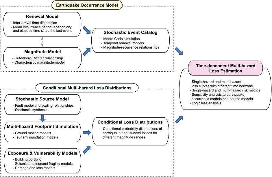
FIGURE 1. Multi-hazard portfolio loss model framework.

TABLE 1

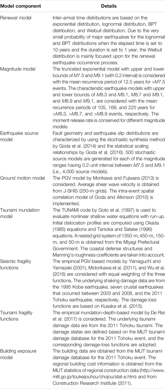
TABLE 1. Components of the time-dependent multi-hazard portfolio loss model for the Tohoku region of Japan.

The first major building block of the portfolio loss model is the generation of stochastic event sets for a specified duration of interest from a set of earthquake occurrence models. The occurrence of major tsunamigenic seismic events is modeled by a renewal process, which captures quasi-periodic characteristics of major tsunamigenic earthquakes (e.g., evens having M7.5 or above) via non-exponential inter-arrival time distributions and the last occurrence of such an event. The magnitude of these major events is characterized by a set of magnitude recurrence models. Popular magnitude models include the truncated exponential model (i.e., G-R relationship) and the characteristic model. The outputs from this model component are numerous stochastic event catalogs of major earthquakes that occur within the specified temporal window (e.g., 1 million catalogs over a 1-year period). In the current model set-up, a physical relationship between the earthquake occurrence and the magnitude is not explicitly captured. In other words, the future earthquake size does not depend on the waiting time (or accumulated stress/strain) since the last event (note: these events still have large magnitudes). More descriptions for the earthquake occurrence model are given in Earthquake Occurrence Model.

The second major building block of the portfolio loss model is the conditional multi-hazard loss distribution. In developing such conditional loss distributions, a magnitude range of interest for the major tsunamigenic events that is considered in the earthquake occurrence model above is discretized into several bins. Subsequently, a stochastic method for earthquake source modeling is used to generate a number of stochastic earthquake rupture models with variable geometry and location and with heterogeneous earthquake slip distribution. To evaluate the hazard footprint of the synthesized stochastic events in terms of shaking intensity and tsunami inundation at building locations of interest, Monte Carlo ground motion and tsunami inundation simulations are implemented for different magnitude ranges. After applying seismic as well as tsunami fragility functions to the building portfolio of interest and relevant damage-loss functions, shaking and tsunami damage severities can be evaluated for both individual buildings and aggregated building portfolio. Eventually, the probability distribution functions of single-hazard and multi-hazard loss metrics can be obtained for different magnitude ranges. More descriptions of the conditional multi-hazard loss distribution are given in Conditional Multi-Hazard Loss Distribution.

To combine the outputs from the first and second major components, for each event in the stochastic event catalogs, the single-hazard and multi-hazard loss values are sampled from the conditional loss distribution that corresponds to the event’s magnitude. For instance, for a seismic event with representative magnitude of 8.6, loss values are sampled from the empirical loss distribution of the 500 stochastic source events that have earthquake magnitudes between M8.5 and M8.7. In this sampling, the dependency of the loss event is maintained, and thus information on the earthquake event characteristics, such as rupture geometry and slip distribution, becomes accessible (Goda and De Risi, 2018). By repeating this loss sampling, the stochastic event catalog can be expanded to include information on the single-hazard and multi-hazard building portfolio loss (i.e., event loss table). Subsequently, statistical analysis can be performed on the event loss table to derive the loss exceedance curves as well as related risk metrics for the building portfolio (Mitchell-Wallace et al., 2017). It is important to emphasize that the time dependency of the shaking and tsunami hazards is retained in the stochastic event sets and thus in the event loss table.

The computational efficiency of the multi-hazard portfolio loss estimation method that is outlined above can be attributed to the decoupling of the earthquake occurrence model and the conditional loss distribution. Simulations of the former component are fast. In contrast, the latter requires significant computations based on a large number of stochastic source models for megathrust subduction events. When the earthquake occurrence model is altered (e.g., different renewal and magnitude models are considered) or extended (e.g., multiple combinations of renewal and magnitude models are considered in a logic tree), the conditional loss distributions do not need to be changed. Moreover, it is noteworthy that instead of resampling the loss quantities from the finite number of stochastic source models, an analytical loss distribution (e.g., Pareto distribution) can be fitted to the simulated conditional loss data. When such analytical models are considered, the direct connection between the loss value and the event characteristics (e.g., earthquake slip distribution) will be lost. Therefore, suitable approaches should be employed depending on the purposes of the developed multi-hazard loss model.

Earthquake Occurrence Model

A stochastic renewal process is adopted for characterizing earthquake occurrence, where the inter-arrival time between successive earthquakes is modeled by some suitable probabilistic model (Ogata, 1999). In this study, four distribution types are considered: i) the exponential distribution is most popular and corresponds to a memory-less Poisson process; ii) the lognormal distribution is often adopted for practical reasons; iii) the BPT distribution can be related to physical phenomena of loading and unloading processes of stress along fault rupture planes (Matthews et al., 2002); and iv) the Weibull distribution is often used for modeling failure times of engineering products and is suitable for representing a process having the increasing hazard function since the last failure (Abaimov et al., 2008). The details of the mathematical formula for these distributions can be found in standard statistical textbooks (see also Goda, 2019).

Three model parameters define the inter-arrival time distribution: the mean recurrence time μ, the aperiodicity ν, and the elapsed time since the last event T_E. The mean recurrence time is typically estimated based on historical earthquake records and geological records (e.g., Ogata, 1999; Ceferino et al., 2020). The ν parameter determines the periodicity of earthquake occurrence. Suitable ν values for large subduction events can be in the range of 0.5 ± 0.2 (Sykes and Menke, 2006). When ν is small (e.g., less than 0.2) the process becomes more periodic, whereas when ν is large the process becomes more random and clustering of the events tends to occur more frequently. The probability distribution of inter-arrival time needs to be modified when T_E is not equal to zero to account for the fact that no major events have occurred to date.

Evaluation of the renewal process can be facilitated through Monte Carlo simulations. In the simulation-based approach, random numbers from a specified inter-arrival time distribution are generated using an inverse transformation method or a rejection method. For the renewal process, a special attention is necessary to distinguish the first event and subsequent events (i.e., T_E ≠ 0 vs. T_E = 0). This is illustrated in Figure 2A. For simulating the occurrence time of the first event, the modified inter-arrival time distribution should be used by taking into account T_E. When the simulated time t_IAT is less than the duration for the hazard assessment T_D, the simulated event should be registered as t₁ = t_IAT in a stochastic event catalog and proceed to the second event; otherwise the simulation process is stopped for this catalog realization. For the second event, the elapsed time is reset to 0 and an inter-arrival time t_IAT is sampled from the original distribution and the occurrence time is updated as t₂ = t₁ + t_IAT. If t₂ is less than T_D, the second event is registered in the stochastic event catalog; otherwise the simulation ends for this catalog realization. This process should be continued until the updated time of the most recent event exceeds T_D. By repeating the simulations of event occurrence S times, a set of S stochastic event catalogs, each with the duration T_D, can be obtained.

FIGURE 2

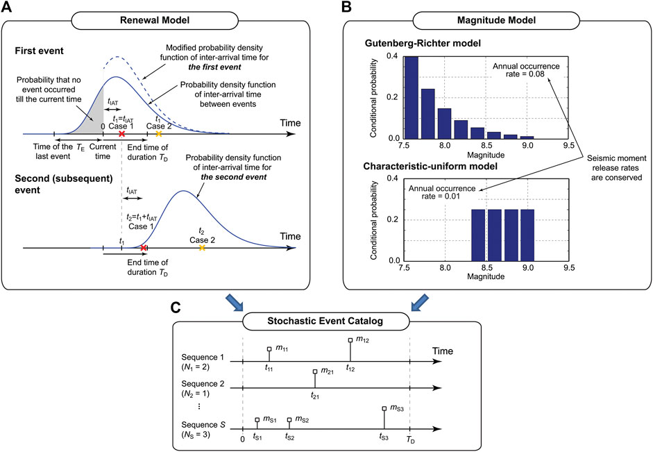
FIGURE 2. Evaluation of earthquake occurrence processes. (A) Renewal model, (B) Magnitude model, (C) Stochastic event catalog.

The magnitude recurrence distribution characterizes the uncertainty of earthquake magnitude when a major event occurs. A popular model is of G-R type, where the overall occurrence rate for major events and the relative distribution of earthquake magnitude (i.e., b-value) are determined from statistical analysis of regional seismicity. Other types of the magnitude model include the characteristic magnitude models with uniform or truncated normal distributions. Figure 2B shows two examples of the magnitude models, namely a G-R model that is defined over a magnitude range between M7.5 and M9.1, whereas a characteristic-uniform model that is defined over a magnitude range between M8.3 and M9.1. It is important to emphasize that the magnitude models should be consistent with regional seismotectonic conditions. As such, the occurrence frequency of major events (i.e., mean recurrence time of the renewal model) needs to be adjusted based on regional seismic moment release constraints, which can be determined from the regional G-R analysis and/or the regional plate movements. For the case of the Tohoku region, the regional G-R analysis indicates the annual occurrence frequency of 0.08 for M7.5 and above events (with b = 0.9; Goda and De Risi, 2018). When the characteristic-uniform model shown in Figure 2B is considered, the annual occurrence frequency is decreased to 0.01.

By simulating the stochastic occurrence process of large subduction events, numerous stochastic event catalogs are obtained. This is illustrated in Figure 2C. Each catalog contains N_i events, i = 1,…,S, and is characterized by the paired information of occurrence time t_ij and magnitude m_ij, j = 1,…,N_i. These simulated earthquake sequences are used in the multi-hazard portfolio loss model. It is noted that when multiple combinations of the renewal and magnitude models are implemented in a logic tree, sampling of the renewal and magnitude model parameters is performed first and then based on the realized parameters, the stochastic event information t and m over a T_D-year period is generated. For a different catalog, the renewal and magnitude model parameters need to be resampled prior to the stochastic event generation.

Conditional Multi-Hazard Loss Distribution

The multi-hazard shaking-tsunami loss for a magnitude range is estimated by integrating five modules: a) stochastic source model, b) shaking-tsunami footprint simulations, c) building exposure model, d) seismic-tsunami vulnerability model, and e) conditional multi-hazard loss estimation. A computational procedure of the conditional multi-hazard loss distributions is illustrated in Figure 3. Brief descriptions of the modules are given below.

FIGURE 3

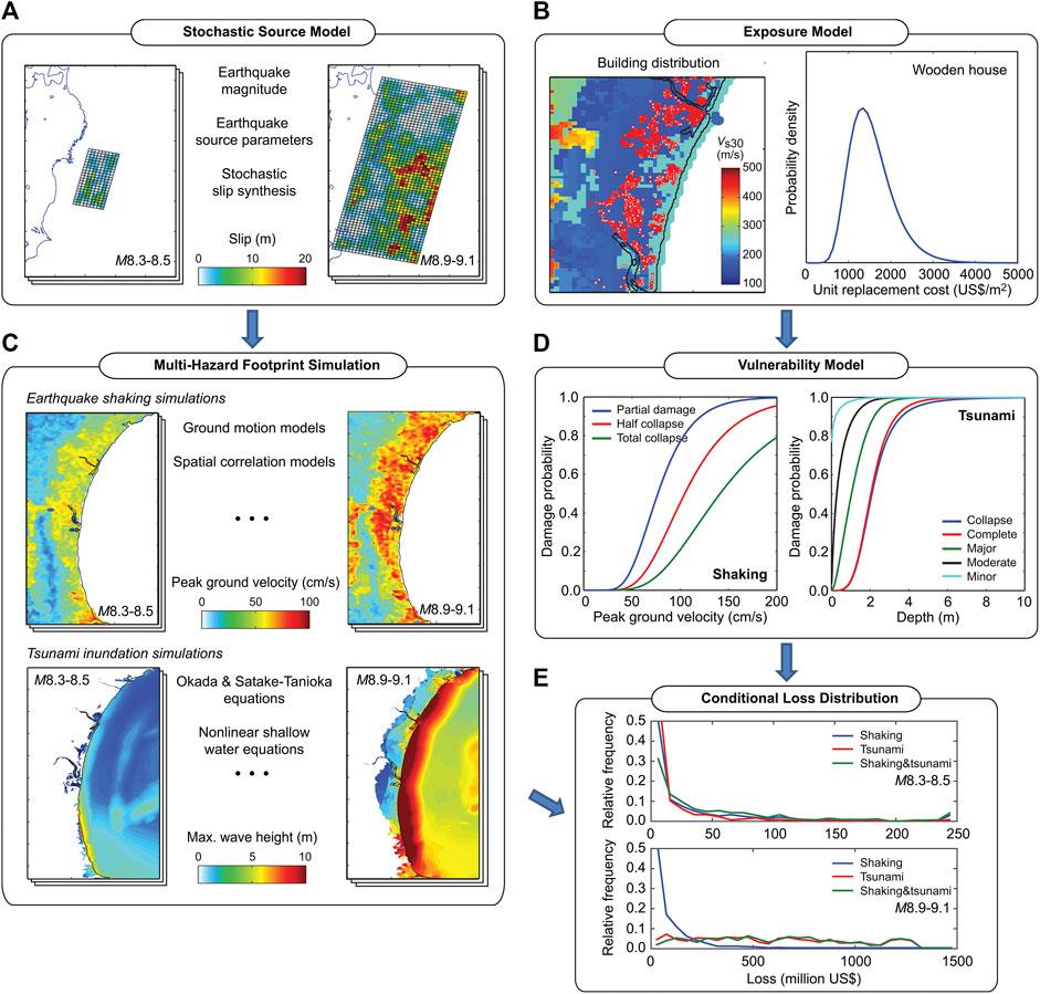
FIGURE 3. Evaluation of conditional shaking-tsunami loss distributions. (A) Stochastic source model, (B) Exposure model, (C) Multi-hazard footprint simulation, (D) Vulnerability model, (E) Conditional loss distribution.

Stochastic Source Model

The stochastic source model captures the spatial uncertainty of earthquake rupture for a given earthquake magnitude (Figure 3A). The model for the Tohoku region of Japan covers an offshore area of 650 by 250 km. The source uncertainty is characterized by probabilistic models of earthquake source parameters and stochastic synthesis of earthquake slip (Goda and De Risi, 2018). For a magnitude value, eight source parameters, i.e., fault width, fault length, mean slip, maximum slip, Box-Cox power parameter, correlation length along dip, correlation length along strike, and Hurst number, are generated using empirical prediction equations based on 226 finite-fault models of the past earthquakes. Once the geometry and position of a stochastic source model are determined, a random heterogeneous slip distribution is generated using a Fourier integral method, where amplitude spectrum is represented by von Kármán spectra and random phase (Mai and Beroza, 2002). To generate a slip distribution with realistic right-heavy tail features, the synthesized slip distribution is converted via Box-Cox power transformation. The transformed slip distribution is then adjusted to achieve the suitable slip characteristics, such as mean slip and maximum slip. In this study, 500 stochastic source models are generated for eight magnitude ranges with 0.2 bin width spanning from M7.5 and M9.1 (i.e., 4,000 models in total). The synthesized earthquake source models reflect possible variability of tsunamigenic earthquakes in terms of geometry, fault location, and slip distribution.

Multi-Hazard Footprint Simulations

For a given earthquake source model, shaking and tsunami hazard intensities at building locations are evaluated by using a ground motion model and by solving non-linear shallow water equations for initial boundary conditions of sea surface caused by an earthquake rupture, respectively (Figure 3B). In this study, the peak ground velocity (PGV) is selected for shaking and the maximum inundation depth is adopted for tsunami. The choice of PGV as seismic hazard measure is due to its compatibility with empirical seismic fragility functions in Japan (see Table 2). The local site conditions are based on the J-SHIS average shear-wave velocity database (http://www.j-shis.bosai.go.jp/en/; 250-m grids). The PGV ground motion model by Morikawa and Fujiwara (2013) together with the intra-event spatial correlation model of Goda and Atkinson (2010) is used to generate spatially correlated ground motion fields for all 4,000 stochastic sources. On the other hand, tsunami inundation and run-up simulations are performed using a well-tested TUNAMI computer code by Goto et al. (1997). The computational domains are nested with 1,350, 450, 150, and 50-m resolution grids. The maximum inundation depths at the building locations are determined by subtracting land elevations from the maximum inundation heights. It is noted that inundation depth does not capture the tsunami flow effects on buildings directly; for such purposes, flow velocity-based tsunami fragility functions can be adopted (De Risi et al., 2017). Tsunami simulations are conducted for all 4,000 stochastic sources by considering duration of 2 h.

TABLE 2

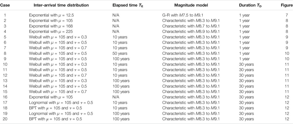
TABLE 2. Numerical calculation cases.

Building Exposure Model

Using a building dataset that was compiled by the Japanese Ministry of Land Infrastructure and Transportation (MLIT) for the post-2011-Tohoku tsunami damage assessment, an exposure model is developed for Iwanuma City and Onagawa Town (Figure 3C). Building types that are considered in this study are low-rise wooden structures (up to 4-story buildings; the majority of the buildings are 1 story or 2 stories), for which well-calibrated seismic and tsunami fragility models are available. The numbers of wooden structures in Iwanuma and Onagawa are 6,152 and 1,706, respectively. To obtain estimates of the building costs for the wooden buildings in Iwanuma and Onagawa, two sources of information are utilized. Using the Japanese building cost information handbook published by the Construction Research Institute (2011) and MLIT building stock database, the mean and CoV of the unit replacement cost for wooden buildings are obtained as 1,600 US$/m2 and 0.33, respectively (assuming 1 US$ = 100 yen), whereas the mean and CoV of typical floor areas of wooden houses are determined as 130 m² and 0.33, respectively. Both unit cost and floor area are modeled by the lognormal distribution. Based on the above building cost information, the expected total costs of the 6,152 buildings in Iwanuma and the 1,706 buildings in Onagawa are 1,280 million US$ and 355 million US$, respectively.

Vulnerability Model

Damage ratios for shaking and tsunami are estimated by applying seismic and tsunami fragility functions (Figure 3D). The seismic fragility models are based on three empirical functions for low-rise wooden buildings in Japan (Yamaguchi and Yamazaki, 2001; Midorikawa et al., 2011; Wu et al., 2016), whereas the tsunami fragility model is based on the tsunami damage data from the 2011 Tohoku earthquake and tsunami (De Risi et al., 2017). The damage states for shaking are defined as: partial damage, half collapse, and complete collapse, and the corresponding damage ratios are assigned as 0.03–0.2, 0.2–0.5, and 0.5–1.0, respectively (Kusaka et al., 2015). For tsunami damage, the following five damage states are considered: minor, moderate, extensive, complete, and collapse, together with the damage ratios of 0.03–0.1, 0.1–0.3, 0.3–0.5, 0.5–1.0, and 1.0, respectively (MLIT, http://www.mlit.go.jp/toshi/toshi-hukkou-arkaibu.html). Subsequently, for each building, a greater of the estimated shaking and tsunami damage ratios is adopted as the final damage ratio of the building. A multi-hazard loss value is calculated by sampling a value of the building replacement cost from the lognormal distribution and then by multiplying it by the final damage ratio. The above-mentioned method of calculating the combined shaking-tsunami damage ratio does not account for interaction between shaking and tsunami damage explicitly. For the current model of the Tohoku region, this limitation is alleviated because the tsunami fragility model by De Risi et al. (2017) is based on tsunami damage data from the 2011 Tohoku event that include the effects due to shaking damage.

Conditional Multi-Hazard Loss Estimation

A numerical procedure of integrating the hazard and risk model components is implemented using Monte Carlo simulations (Goda and De Risi, 2018; Figure 3E). At the end of the simulation, loss samples for all buildings are obtained for the 4,000 stochastic source models. These loss samples can be used to construct the conditional distribution functions of the total portfolio loss for different magnitude ranges.

One of the notable features of the developed multi-hazard shaking-tsunami loss estimation is the consideration of variable fault geometry and heterogeneous earthquake slip distribution. The latter is particularly influential on tsunami hazard predictions (Goda et al., 2016). To illustrate this effect on tsunami loss, cumulative probability distributions of tsunami loss for Iwanuma and Onagawa are shown in Figure 4 by considering heterogeneous slip distributions and uniform slip distributions. The cumulative probability distributions are developed for the eight magnitude ranges to better distinguish the loss results in terms of earthquake magnitude (i.e., conditional tsunami loss distribution). The heterogeneous slip distributions take into account variability in both fault geometry and spatial slip distribution, whereas the uniform slip distributions reflect variability of fault geometry only but with average slip across the fault plane (note: for a given earthquake source model, the earthquake magnitude is identical for the heterogeneous and uniform slip cases). Figure 4 clearly shows the effects of spatial slip distribution and the consideration of realistic heterogeneous slip distributions results in significantly greater and more variable conditional tsunami loss distributions than uniform slip distributions. This is in agreement with the previous studies (Mueller et al., 2015; Li et al., 2016; Melgar et al., 2019). For instance, for the building portfolio in Iwanuma (Figures 4A,B), probability that the tsunami loss exceeds 600 million US$ is circa 0.5 for the heterogeneous slip case, whereas that probability for the uniform slip case is approximately 0.1.

FIGURE 4

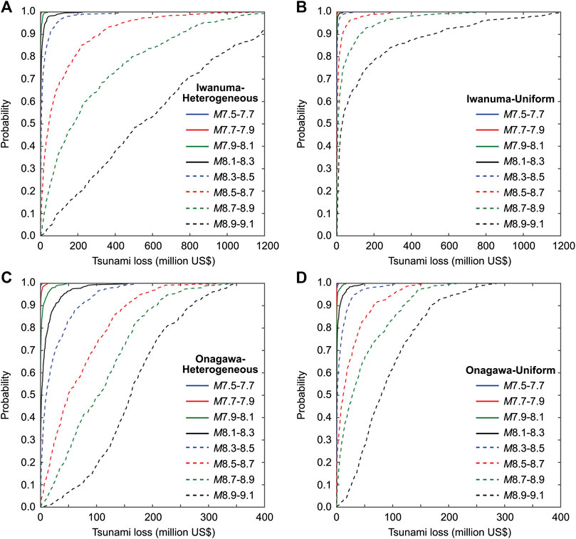
FIGURE 4. Cumulative probability distributions of tsunami loss for the building portfolios in Iwanuma (A,B) and Onagawa (C,D) by considering heterogeneous distributions (A,C) and uniform distributions (B,D) of earthquake slip.

As mentioned in Computational Framework, the computational efficiency of the proposed multi-hazard loss estimation procedure depends on the stability of the conditional loss distributions for the magnitude ranges. In other words, the sample size of stochastic source models per magnitude bin should be sufficiently large. To examine whether such stable loss distributions are achieved for the case studies that are discussed in Results, the five percentiles (2.5th, 16th, 50th, 84th, and 97.5th) of shaking loss, tsunami loss (with heterogeneous or uniform slip distributions), and combined loss (with heterogeneous or uniform slip distributions) for Iwanuma and Onagawa are displayed as a function of the number of stochastic source models. For illustration, the magnitude range between M8.3 and M8.5 is considered in Figure 5. It can be observed that with 300 or more source models, the conditional loss distributions become stable for this magnitude bin. Similar stabilizing trends are observed for different magnitude bins (not reported in the paper). It is important to note that the stability of the conditional loss distributions depends on the target metric that is adopted for the investigation. When a portfolio-aggregated loss is concerned (as in this study), the sum of losses of individual buildings fluctuate less, compared to a loss of a particular building. Therefore, for the latter case, it may require more stochastic source models to achieve such stability.

FIGURE 5

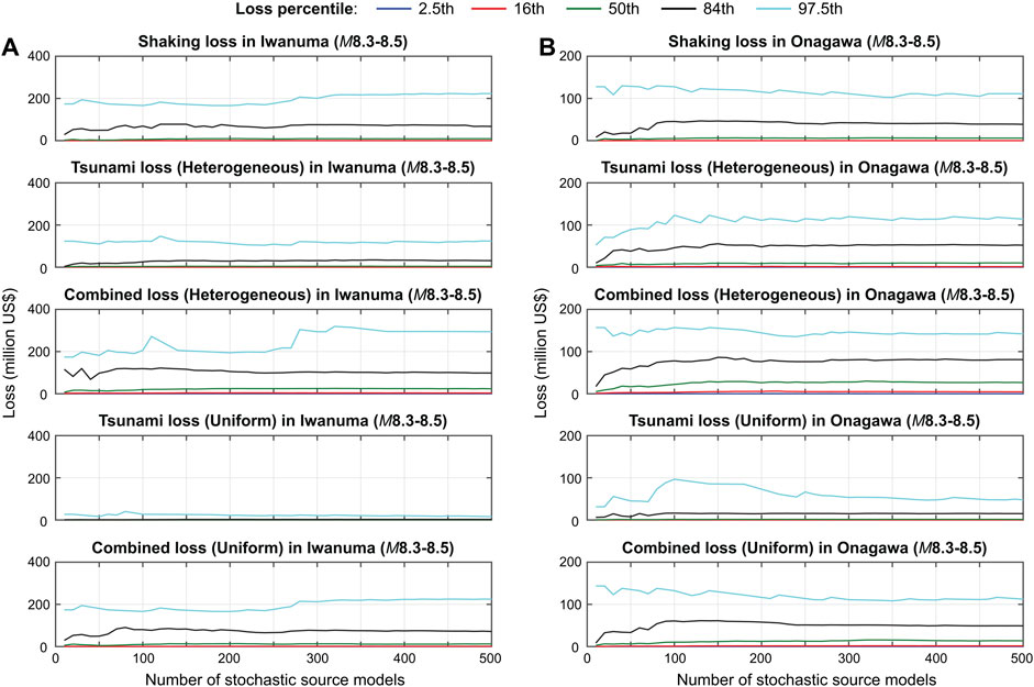
FIGURE 5. Stability of conditional loss distributions for the building portfolios in Iwanuma (A) and Onagawa (B) due to stochastic source models with magnitudes between M8.3 and M8.5.

Model Limitations

The multi-hazard portfolio loss estimation framework for time-dependent shaking and tsunami hazards presented in this section has limitations and is specific to the case study region in Japan. The region-specific modules include applicable earthquake occurrence models, earthquake source characteristics (overall fault geometry and source parameters), ground motion models for seismic intensity parameters, regional and local factors that affect tsunami inundation (e.g., bathymetry and elevation), seismic and tsunami fragility functions, and exposure databases (e.g., building cost and design information). Some of the model choices are constrained by other modules (for example, the use of PGV in ground motion modeling is prescribed by seismic hazard measures used in seismic fragility functions, whereas unavailability of seismic fragility functions for non-wooden building typologies leads to exclusion of non-wooden buildings in the exposure model).

Some of the limitations of the developed multi-hazard loss model are listed in the following. These are not the complete list of the limitations and each of these is worthy of future investigations.

• In modeling interaction between spatiotemporal earthquake occurrence and magnitude, a simple renewal process is adopted in this work. Time-predictable and slip-predictable models by Shimazaki and Nakata (1980) and Kiremidjian and Anagnos (1984), respectively, can capture causal relationships between the inter-arrival time and magnitude. When the subduction zone is divided into several distinct segments, the space- and time-interaction model by Ceferino et al. (2020) can be implemented.

• The framework only considers a single source region (i.e., offshore Tohoku region), while other sources that could cause major destruction to the building portfolio can be incorporated. Such additional sources include crustal and inslab seismic sources for shaking damage and far-field tsunami sources for tsunami damage (e.g., Cascadia and Chile subduction zones for the Tohoku region).

• Although the tsunami footprint simulation is performed by solving the nonlinear shallow water equations, ground motion simulation is based on empirical statistical model of ground motion intensity. When a high-resolution 3D crustal velocity model is available and more computational resources are dispensable, hybrid ground motion simulations (Pitarka et al., 2017; Frankel et al., 2018) can be implemented to incorporate more physical features in the evaluation of ground shaking intensity.

• In assessing the damage extent of a building subjected to a sequence of shaking and tsunami hazards, the damage accumulation of the cascading hazards becomes an important factor. Such a damage accumulation model can be developed based on reliable numerical models of structures by subjecting these models to a sequence of shaking-tsunami loads (Park et al., 2012).

Results

Numerical Calculation Set-Up

Two case study locations are considered for the exposure model. Iwanuma is located on the Sendai plain, whereas Onagawa is located along the Sanriku ria coast. Both locations were devastated during the 2011 Tohoku earthquake and tsunami (Fraser et al., 2013). Figures 6A,B show the spatial distributions of buildings in Iwanuma and Onagawa, respectively. The markers shown in the figure are color-coded with actual building damage states assigned by the MLIT after the 2011 Tohoku event. In addition, histograms of the damage for Iwanuma and Onagawa are shown in Figures 6C,D, respectively. Different spatial patterns of building damage, which essentially reflect the tsunami inundation extents at these two locations, can be observed. With the increase of distance from the coastal line, the damage states in Iwanuma become less severe as the inundation depths become smaller. In contrast, the collapse damage states in Onagawa are prevalent across nearly all buildings that are located in the valley because of the very high inundation heights exceeding 18 m (Fraser et al., 2013). By applying the same damage-loss functions introduced in Conditional Multi-Hazard Loss Distribution, the total damage costs for the buildings in Iwanuma and Onagawa are calculated as 743 million US$ and 337 million US$, respectively, which are equal to the average loss ratio of 58 and 95% for the 2011 Tohoku event. These empirical results indicate that the occurrence of catastrophic loss is for real for these two locations.

FIGURE 6

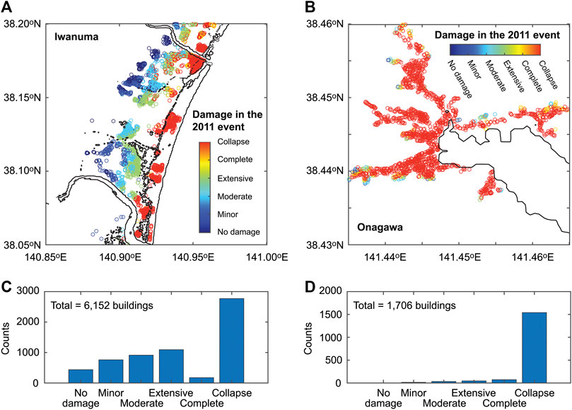
FIGURE 6. Building portfolios in Iwanuma (A) and Onagawa (B). The colors represent the MLIT damage survey results after the 2011 Tohoku earthquake and tsunami. Histograms of damage states of the considered buildings after the 2011 Tohoku earthquake and tsunami for Iwanuma and Onagawa are shown in (C) and (D), respectively.

The main aim of this paper is to investigate the effects of considering different renewal and magnitude models, in comparison with the conventional time-dependent counterpart. To facilitate such comparisons of the results, the baseline result is set to the case of the time-independent multi-hazard loss estimation (Goda and De Risi, 2018; Time-Independent Multi-Hazard Loss Estimation), which adopts the Poisson process and the G-R magnitude model (Case 1). Several variations for the magnitude models are considered by keeping the time-independent occurrence model (Cases 2 to 4). Subsequently, results for the time-dependent cases are discussed to conduct sensitivity analyses for time-dependent multi-hazard loss estimation (Sensitivity Analysis of Time-Dependent Multi-Hazard Loss Estimation). Cases 5 to 7 consider Weibull-based renewal models with different ν values. Cases 8 and 9 adopt different elapsed times since the last major event (T_E = 10, 50, and 100 years; note that T_E = 10 years corresponds to the current situation since the 2011 event). For Cases 1 to 9, the duration of the multi-hazard loss estimation is set to T_D = 1 year. In contrast, a longer time horizon of T_D = 30 years is considered for Cases 10 to 15 by varying both values of T_E and ν. Moreover, Cases 16 to 20 are set up to investigate the effects of using different inter-arrival time distributions (Weibull, lognormal, and BPT) for T_D = 30 years. These calculation cases are summarized in Table 2. For each case, 10 million T_D-year stochastic event catalogs are generated, and the maximum combined loss event in each T_D-year catalog is adopted as a loss metric in developing the single-hazard and multi-hazard loss curves.

Time-independent Multi-Hazard Loss Estimation

Figure 7 shows single-hazard and multi-hazard loss curves for Iwanuma and Onagawa based on the time-independent earthquake occurrence model (Case 1). The consideration of different earthquake slip representations (i.e., heterogeneous vs. uniform) results in significantly different tsunami loss curves as well as combined loss curves (see also Figure 4). The shaking loss is not affected by the differences of the earthquake slip representation because in the context of ground motion modeling, the fault geometry only affects the predicted ground motion intensities. At higher annual exceedance probability levels (shorter return periods), shaking loss contributes more to the combined loss, whereas at lower annual exceedance probability levels (longer return periods), tsunami loss dominates the combined loss. The changeover of the loss-origin dominance depends significantly on the earthquake slip representation. This difference can be explained by different hazard characteristics for ground shaking and tsunami. Ground motion intensity at a specific location tends to be saturated in terms of earthquake magnitude (Morikawa and Fujiwara, 2013), although areas that experience intense shaking increase rapidly due to the expanding rupture size). On the other hand, tsunami inundation height and spatial extent increase rapidly with earthquake magnitude; devastating inundations of coastal plain areas like Iwanuma happen very rarely (as seen during the 2011 Tohoku event; Fraser et al., 2013). In short, the coastal topography (plain vs. ria) is one of the crucial factors that determine how frequent and how severe the tsunami damage and loss will turn out to be.

FIGURE 7

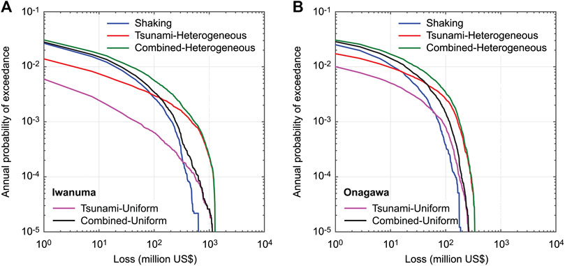
FIGURE 7. Single-hazard and multi-hazard loss curves for Iwanuma (A) and Onagawa (B) based on the time-independent earthquake occurrence model (Case 1).

For very large earthquakes, different magnitude models may be more applicable. To investigate the effects of different magnitude models on the single-hazard and multi-hazard loss curves, three characteristic magnitude models with uniform distribution are considered by varying the lower-bound magnitudes from M8.3 to M8.9. Accordingly, the mean recurrence period of major earthquakes is changed from 105 to 225 years by conserving the seismic moment release from the specified source region based on the regional G-R model (see Table 2).

Figure 8 shows single-hazard and multi-hazard loss curves for Iwanuma and Onagawa by considering different magnitude models (Cases 1 to 4); to facilitate the inspection of the results, shaking, tsunami, and combined loss curves are presented in separate figure panels. With the consideration of more characteristic behavior of the magnitude distribution, shorter return-period portions of the shaking loss curves are shifted down from the annual probability of exceedance of 0.02 to 0.004 due to longer mean recurrence periods of major events (Figures 8A,B). Longer return-period portions of the shaking loss curves are not affected by the different magnitude models because of the fixed upper magnitude limit at M9.1 and the magnitude saturation in the ground motion model.

FIGURE 8

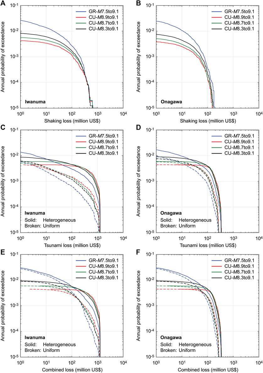
FIGURE 8. Single-hazard and multi-hazard loss curves for Iwanuma (A,C,E) and Onagawa (B,D,F) by considering different characteristic-uniform (CU) magnitude models (Cases 1 to 4).

The tsunami loss curves (Figures 8C,D) show the influence of the magnitude model at both ends of the loss curves. The shorter return-period portions of the tsunami loss curves are affected by the mean recurrence periods of major events (the same reason for the shaking loss curves). On the other hand, severe tsunami loss curves are resulted from the consideration of more characteristic behavior of the magnitude model. The effects of the earthquake slip distribution are noticeable for different magnitude models, especially remarkable for Iwanuma.

The multi-hazard loss curves (Figures 8E,F) exhibit combined effects from the shaking loss curves and tsunami loss curves, as discussed above. The consideration of the characteristic magnitude model results in more severe combined loss curves at annual exceedance probability levels lower than 0.01. These increased levels of the multi-hazard loss for the building stock in Iwanuma and Onagawa indicate the importance of considering a range of magnitude models for disaster risk management purposes. In Sensitivity Analysis of Time-dependent Multi-Hazard Loss Estimation, the characteristic magnitude model with uniform distribution between M8.3 and M9.1 is adopted to further investigate the effects of adopting different earthquake occurrence models on the multi-hazard loss estimation.

Sensitivity Analysis of Time-dependent Multi-Hazard Loss Estimation

Effects of different earthquake occurrence models are investigated in this section. More specifically, the effects of aperiodicity parameter are examined in Sensitivity to Aperiodicity Parameter by adopting the Weibull inter-arrival time distribution for T_E = 10 years (current situation) and T_D = 1 year. Note that for T_E = 10 years and T_D = 1 year, when the lognormal and BPT distributions are considered, the loss estimation results are nearly zero due to very small probabilities of earthquake occurrence within the specified time window; for this reason, the Weibull distribution is mainly focused upon. Subsequently, the effects of the elapsed time since the last major event are evaluated in Sensitivity to Elapsed Time Since the Last Major Event by considering hypothetical future situations of T_E = 50 and 100 years (T_D = 1 year). In Sensitivity to Time Window Length, the impact of considering a longer time window for the loss estimation is investigated by considering T_D = 30 years. The time window length of 30 years is often considered in Japan for long-term earthquake disaster risk mitigation purposes (e.g., national seismic hazard maps). Lastly, the effects of different inter-arrival time distributions are examined in Sensitivity to Inter-Arrival Time Distribution by considering the time horizon of T_D = 30 years.

Sensitivity to Aperiodicity Parameter

Figure 9 compares single-hazard and multi-hazard loss curves for Iwanuma and Onagawa by considering Weibull-based renewal models with different aperiodicity values of ν = 0.3, 0.5, and 0.7 (Cases 5 to 7), which fall within the empirical estimates of this parameter for global subduction zones (Sykes and Menke, 2006). The inter-arrival time distribution is based on the Weibull model with mean recurrence period of 105 years (for M8.3 to M9.1 events) and T_E is set to 10 years. For the baseline comparison, the loss curves for Case 1 are included. The effects of the time-dependent hazards are paramount, changing the positions of the loss curves by a factor of 100 times in terms of annual probability of exceedance (from ν = 0.3 to ν = 0.7).

FIGURE 9

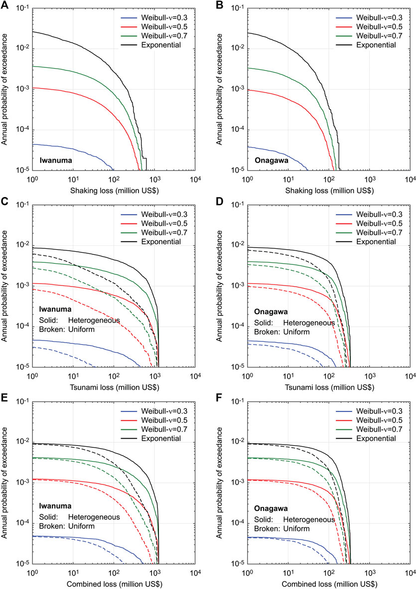
FIGURE 9. Single-hazard and multi-hazard loss curves for Iwanuma (A,C,E) and Onagawa (B,D,F) by considering Weibull-based renewal models with different ν values (Cases 2, 5, 6, and 7).

Results for the shaking loss curves (Figures 9A,B) show that the loss curves for the time-dependent occurrence models are less risky than those for the time-independent occurrence model and with the increase in ν, the loss curves for the time-dependent occurrence models approach that of the time-independent occurrence model. This can be explained by the fact that the current time instance (T_E = 10 years) is shorter than the mean recurrence period (μ = 105 years) and is still in the early phase of stress accumulation process of major subduction events. Therefore, the less periodic earthquake occurrence behavior (i.e., larger ν values) results in greater occurrence probability of major events within a time window of 1 year.

The same observations are applicable to the tsunami loss curves and combined loss curves shown in Figures 9C–F). Essentially, respective loss curves are shifted down according to the occurrence probabilities of major events. Overall, the effects of aperiodicity parameter (i.e., steepness of the inter-arrival time distribution around mean) are significant, especially for the early phase of the renewal process. Since the effects of the time-dependent occurrence model are qualitatively identical to shaking, tsunami, and combined loss curves (for the same magnitude model), the multi-hazard loss curves are mainly discussed in the following.

Sensitivity to Elapsed Time Since the Last Major Event

Different temporal phases within a renewal process lead to different risk estimates of the time-dependent hazards. To investigate this aspect, hypothetical values of T_E = 50 and 100 years (Cases 8 and 9) are considered and their combined loss curves for Iwanuma and Onagawa are compared in Figure 10 with the time-independent occurrence case (Case 2) and the time-dependent occurrence case for the current situation (Case 5). The time window length is 1 year and the ν value for the time-dependent cases is set to 0.5. Considering a longer elapsed time since the last major event results in significant increase of the multi-hazard loss by changing the positions of the loss curves by a factor of 10 times or more in terms of annual probability of exceedance.

FIGURE 10

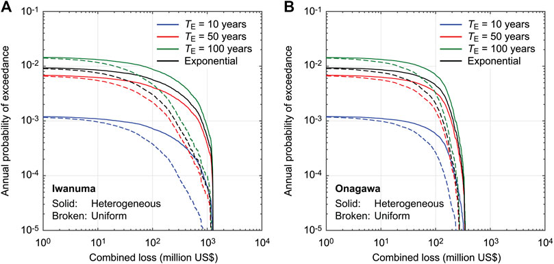
FIGURE 10. Multi-hazard loss curves for Iwanuma (A) and Onagawa (B) by considering Weibull-based renewal models with different T_E values (Cases 2, 5, 8, and 9).

The results shown in Figure 10 indicate that when the intermediate temporal phase is reached (T_E = 50 years), the combined loss curves for the time-dependent (red) and time-independent (black) cases become similar. When major events are overdue (T_E = 100 years), the time-dependent loss curves exceed the time-independent counterparts. It is important to note that the observations made for Figure 10 are specific to the numerical set-up of the models considered. In other words, they should not be generalized since the results depend other parameters, such as mean recurrence period (i.e., magnitude model) and aperiodicity parameter.

Sensitivity to Time Window Length

The time horizon of the multi-hazard loss estimation depends on the purposes of such quantitative risk assessments as well as the types of disaster risk mitigation planning and actions. As such, a longer time window of T_D = 30 years is chosen. To examine the effects of aperiodicity parameter in tandem with different elapsed times since the last major event, multi-hazard loss curves for Iwanuma and Onagawa are compared in Figure 11 by considering Weibull-based renewal models with ν = 0.3, 0.5, and 0.7 (Cases 10 to 15). Figures 11A,B are based on T_E = 10 years (current), whereas Figures 11C,D are based on T_E = 100 years (hypothetical). Note that the vertical axis of the loss curves in Figure 11 corresponds to 30-year probability of exceedance, and thus the direct comparisons with other previous figures are not possible.

FIGURE 11

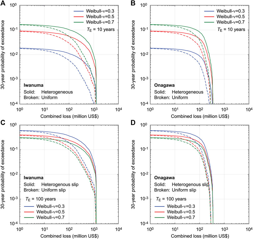
FIGURE 11. Multi-hazard loss curves for Iwanuma (A,C) and Onagawa (B,D) by considering Weibull-based renewal models with different T_E and ν values (Cases 10 to 15). The duration of the stochastic event catalogs is set to T_D = 30 years.

When T_E is set to 10 years (Figures 11A,B), qualitatively, the observations made for Figure 9 are applicable. Because the longer time window is considered, the differences of occurrence probability of major events are less dramatic (approximately increase by a factor of 10 in terms of annual probability of exceedance from ν = 0.3 to ν = 0.7), thereby the loss curves are more similar. The order of the loss curves in terms of ν is the same as that shown in Figure 9, i.e., loss curves become greater with the increase in ν.

When the cases with T_E = 100 years are inspected (Figures 11C,D), the loss curves are increased with respect to those for T_E = 10 years and the differences of the loss curves due to different ν values become relatively less noticeable (by a factor of 2), in comparison with the cases with T_E = 10 years. It is also important to note that the order of the loss curves in terms of ν is now reversed with respect to that for T_E = 10 years. This happens because with the smaller ν value (i.e., more periodic behavior) and the overdue situation of the renewal process (T_E ≈ μ), the probability of major events within the considered time window becomes greater.

Sensitivity to Inter-arrival Time Distribution

The last crucial model component of a renewal process is the inter-arrival time distribution. This component is varied by considering T_D = 30 years. Four inter-arrival time distributions are considered: exponential (i.e., time-independent, case 16), Weibull (this model is used as a reference inter-arrival time distribution in the previous cases, Cases 12 and 14), lognormal (Cases 17 and 19), and BPT (Cases 18 and 20). The ν value is set to 0.5 for all time-dependent occurrence models but T_E is changed to either 10 years (current) or 100 years (hypothetical). The results of these cases are compared in Figure 12.

FIGURE 12

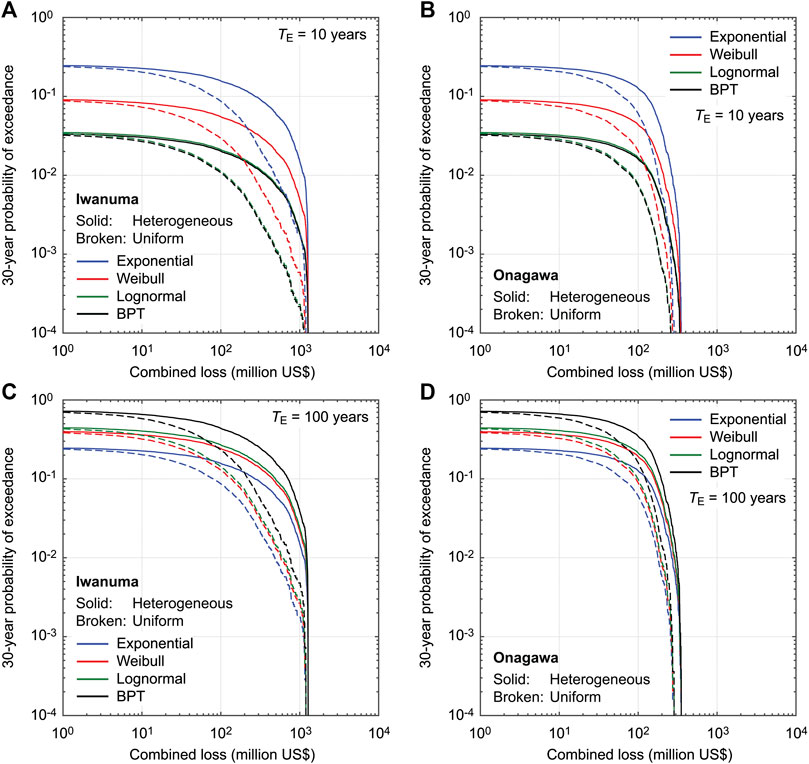
FIGURE 12. Multi-hazard loss curves for Iwanuma (A,C) and Onagawa (B,D) by considering different inter-arrival time distributions with T_E = 10 and 100 years and ν = 0.5 (Cases 12, 14, and 16 to 20). The duration of the stochastic event catalogs is set to T_D = 30 years.

The results for the cases with T_E = 10 years (Figures 12A,B) show that the time-dependent loss estimation for the current situation leads to overestimation of the multi-hazard loss (by a factor of nearly 10). The same situation is demonstrated in Figure 10 for T_D = 1 year. It can be observed that the loss curves based on the lognormal and BPT models lead to smaller loss curves compared to those based on the Weibull model (being consistent with the remarks made above for T_D = 1 year). When a hypothetical future situation of T_E = 100 years is considered, the loss curves for the time-dependent cases exceed that for the time-independent case, which is also observed in Figure 10 for T_D = 1 year. Importantly, the order of the loss curves is changed from BPT ≈ lognormal < Weibull < exponential for the case of T_E = 10 years to exponential < Weibull ≈ lognormal < BPT for the case of T_E = 100 years. The differences of the loss curves for different inter-arrival time distributions are noticeable.

Logic-Tree Analysis of Time-dependent Multi-Hazard Loss Estimation

Overall, the results and observations discussed previously in relation to Figures 8–12 clearly indicate that all individual model components (i.e., mean recurrence period, aperiodicity, elapsed time since the last major event, time horizon window, and inter-arrival time distribution) can have major influence on the occurrence probability of major events. In addition, interaction between different components also plays an important role in calculating such probabilities. Given that some of these model parameters are difficult to constrain based on regional seismicity data alone, it is essential to capture a range of plausible earthquake occurrence models when time-dependent multi-hazard loss estimation is conducted, in light of available data and state of the art knowledge.

To explore the extent of epistemic uncertainty associated with the time-dependent earthquake occurrence model, three characteristic magnitude models considered in Cases 2 to 4, three ν values considered in Cases 5 to 7, and two earthquake slip representations of heterogeneous and uniform slips are implemented in a logic tree (i.e., 18 cases). The inter-arrival time distribution is set to the Weibull model and the time window length is fixed at T_D = 1 year, whereas the elapsed time since the last major event is varied: T_E = 10, 50, and 100 years (as considered in Cases 8 and 9). The weights assigned to the characteristic magnitude models with the lower limits of M8.3, M8.7, and M8.9 are 0.4, 0.3, and 0.3, respectively. The weights for the ν values of 0.3, 0.5, and 0.7 are assigned as 0.3, 0.4, and 0.3, respectively. Equal weighting of the heterogenous and uniform slip distributions is considered. It is noted that the selection of models and parameter sets is limited and the assigned logic-tree weights are chosen arbitrarily for demonstration only. In actual shaking-tsunami hazard and risk assessments, a wider range of logic-tree branches should be considered and their weights need to be scrutinized. This is beyond the scope of this study.

Figure 13 shows multi-hazard loss curves for Iwanuma and Onagawa by considering the above-mentioned logic tree with different T_E values of 10, 50, and 100 years. The individual loss curves are shown with gray color, while the mean, median, and 16th/84th percentile loss curves are shown with solid-red, solid-blue, and broken-blue lines, respectively. For benchmarking purpose, the corresponding loss curves for the heterogenous and uniform slip distributions are also included in the figures (solid/broken-magenta lines). It is noted that for the case of T_E = 10 years (Figures 13A,B), the 16th percentile curves lie outside of the graph area and thus are not shown.

FIGURE 13

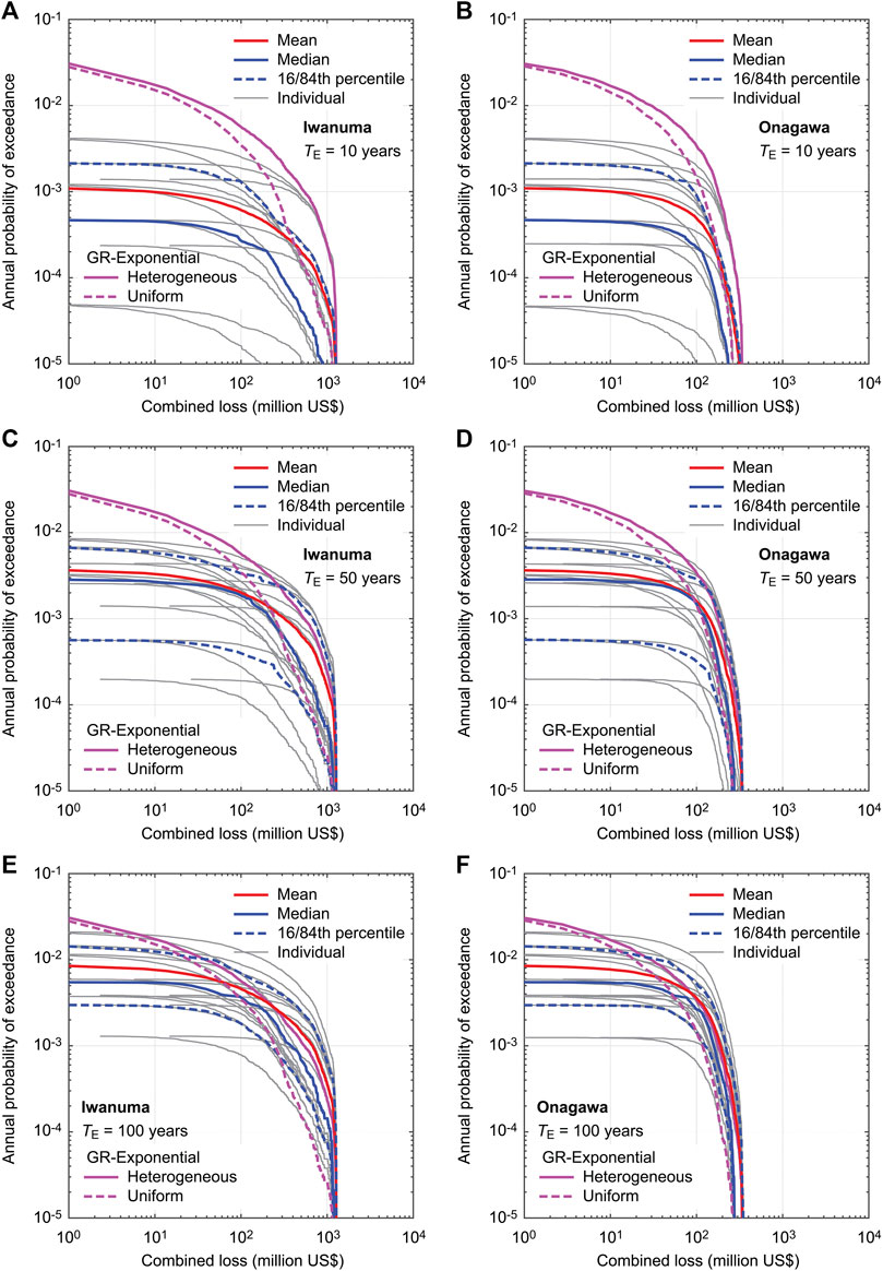
FIGURE 13. Multi-hazard loss curves for Iwanuma (A,C,E) and Onagawa (B,D,F) by considering a logic tree with different T_E values of 10, 50, and 100 years.

The results for T_E = 10 years (Figures 13A,B) show a wide variation of individual curves, all of which are below the time-independent loss curves. The minimum and maximum of the individual curves differ by a factor of 100 or more in terms of annual probability of exceedance (depending on the loss levels). The significant range of the results reflects the sensitivity of the time-dependent multi-hazard loss curves to the characteristics of the renewal processes considered (e.g., mean recurrence period and aperiodicity), especially in the early phase of the renewal process. With the longer elapsed time of T_E = 50 years (Figures 13C,D), the individual loss curves are all shifted upwards and their mean and median curves become more consistent with the time-independent loss curves in a broad sense. Notably, the variation of the individual loss curves is significantly reduced (a factor of circa 20 in terms of annual probability of exceedance), compared with the case of T_E = 10 years. The above-mentioned tendency of the decreased variation of the individual loss curves becomes more obvious for the case of T_E = 100 years (Figures 13E,F), although many of individual cases tend to exceed the corresponding time-independent loss curves, except for annual exceedance probability levels higher than 0.01. An important observation from Figure 13 is that the extent of epistemic uncertainty associated with time-dependent earthquake occurrence model depends on the elapsed time since the last major event, which is more fundamentally related to the corresponding phase of the temporal occurrence process.

Conclusions

Shaking and tsunami hazards caused by megathrust subduction earthquakes are time-dependent. Thereby, a suitable modeling framework is needed when multi-hazard risks to coastal communities are concerned. This study developed a novel catastrophe model for time-dependent seismic and tsunami hazards by adopting a renewal process for the earthquake occurrence model. The developed multi-hazard loss model was applied to the two case study locations in Miyagi Prefecture, Japan, having different topographical features. A series of sensitivity analyses was performed by altering the key elements of the renewal process, including mean recurrence period (via different magnitude models), aperiodicity parameter, elapsed time since the last major event, time window, and inter-arrival time distribution. The sensitivity analysis results highlight not only the significant influences of individual model components but also the impact of their interaction. The results indicate that the time-dependent earthquake occurrence model should be specified carefully and should account for a range of parameter combinations in a logic tree. Another important observation from the numerical results was that the degree of epistemic uncertainty associated with temporal earthquake occurrence changes with time. Noteworthily, the developed multi-hazard modeling approach for time-dependent shaking and tsunami hazards will enable new applications for evaluating financial risks due to subduction earthquakes and tsunamis at community and regional scales and can be further improved by overcoming the current limitations of the methods.

Data Availability Statement

The raw data supporting the conclusions of this article will be made available by the authors, without undue reservation.

Author Contributions

The author confirms being the sole contributor of this work and has approved it for publication.

Funding

The work was supported by the Canada Research Chair program (950-232015) and the NSERC Discovery Grant (RGPIN-2019-05898).

Conflict of Interest

The authors declare that the research was conducted in the absence of any commercial or financial relationships that could be construed as a potential conflict of interest.

References

Abaimov, S. G., Turcotte, D. L., Shcherbakov, R., Rundle, J. B., Yakovlev, G., Goltz, C., et al. (2008). Earthquakes: recurrence and interoccurrence times. Pure Appl. Geophys. 165, 777–795. doi:10.1007/s00024-008-0331-y. CrossRef Full Text

Google Scholar

Ceferino, L., Kiremidjian, A., and Deierlein, G. (2020). Probabilistic space- and time-interaction modeling of mainshock earthquake rupture occurrence. Bull. Seismol. Soc. Am. 110, 2498–2518. doi:10.1785/0120180220. CrossRef Full Text

Google Scholar

Construction Research Institute (2011). Japan Building Cost Information 2011. Tokyo, Japan, 547.

Google Scholar

Daniell, J. E., Schaefer, A. M., and Wenzel, F. (2017). Losses associated with secondary effects in earthquakes. Front. Built Environ. 3, 30. doi:10.3389/fbuil.2017.00030. CrossRef Full Text

Google Scholar

De Risi, R., Goda, K., Yasuda, T., and Mori, N. (2017). Is flow velocity important in tsunami empirical fragility modeling? Earth Sci. Rev. 166, 64–82. doi:10.1016/j.earscirev.2016.12.015. CrossRef Full Text

Google Scholar

Field, E. H., and Jordan, T. H. (2015). Time‐dependent renewal‐model probabilities when date of last earthquake is unknown. Bull. Seismol. Soc. Am. 105, 459–463. doi:10.1785/0120140096. CrossRef Full Text

Google Scholar

Frankel, A., Wirth, E., Marafi, N., Vidale, J., and Stephenson, W. (2018). Broadband synthetic seismograms for magnitude 9 earthquakes on the Cascadia megathrust based on 3D simulations and stochastic synthetics, Part 1: methodology and overall results. Bull. Seismol. Soc. Am. 108, 2347–2369. doi:10.1785/0120180034. CrossRef Full Text

Google Scholar

Fraser, S., Raby, A., Pomonis, A., Goda, K., Chian, S. C., Macabuag, J., et al. (2013). Tsunami damage to coastal defences and buildings in the March 11th 2011 Mw 9.0 Great East Japan earthquake and tsunami. Bull. Earthq. Eng. 11, 205–239. doi:10.1007/s10518-012-9348-9. CrossRef Full Text

Google Scholar

Fukutani, Y., Suppasri, A., and Imamura, F. (2015). Stochastic analysis and uncertainty assessment of tsunami wave height using a random source parameter model that targets a Tohoku-type earthquake fault. Stoch. Environ. Res. Risk Assess. 29, 1763–1779. doi:10.1007/s00477-014-0966-4. CrossRef Full Text

Google Scholar

Goda, K., and Atkinson, G. M. (2010). Intraevent spatial correlation of ground-motion parameters using SK-net data. Bull. Seismol. Soc. Am. 100, 3055–3067. doi:10.1785/0120100031. CrossRef Full Text

Google Scholar

Goda, K., and Atkinson, G. M. (2014). Variation of source-to-site distance for megathrust subduction earthquakes: effects on ground motion prediction equations. Earthq. Spectra. 30, 845–866. doi:10.1193/080512eqs254m. CrossRef Full Text

Google Scholar

Goda, K., and De Risi, R. (2018). Multi-hazard loss estimation for shaking and tsunami using stochastic rupture sources. Int. J. Disaster Risk Reduct. 28, 539–554. doi:10.1016/j.ijdrr.2018.01.002. CrossRef Full Text

Google Scholar

Goda, K., and Hong, H. P. (2006). Optimal seismic design for limited planning time horizon with detailed seismic hazard information. Struct. Saf. 28, 247–260. doi:10.1016/j.strusafe.2005.08.001. CrossRef Full Text

Google Scholar

Goda, K., Mai, P. M., Yasuda, T., and Mori, N. (2014). Sensitivity of tsunami wave profiles and inundation simulations to earthquake slip and fault geometry for the 2011 Tohoku earthquake. Earth Planets Space. 66, 105. doi:10.1186/1880-5981-66-105. CrossRef Full Text

Google Scholar

Goda, K. (2019). Time-dependent probabilistic tsunami hazard analysis using stochastic rupture sources. Stoch. Environ. Res. Risk Assess. 33, 341–358. doi:10.1007/s00477-018-1634-x. CrossRef Full Text

Google Scholar

Goda, K., Yasuda, T., Mori, N., and Maruyama, T. (2016). New scaling relationships of earthquake source parameters for stochastic tsunami simulation. Coast Eng. J. 58, 1650010. doi:10.1142/s0578563416500108 CrossRef Full Text

Google Scholar

Goto, C., Ogawa, Y., Shuto, N., and Imamura, F. (1997). Numerical method of tsunami simulation with the leap-frog scheme. IOC Manual, Paris, France: UNESCO, Technical No. 35.

Google Scholar

Grezio, A., Babeyko, A., Baptista, M. A., Behrens, J., Costa, A., Davies, G., et al. (2017). Probabilistic tsunami hazard analysis: multiple sources and global applications. Rev. Geophys. 55, 1158, doi:10.1002/2017RG000579. CrossRef Full Text

Google Scholar

Kajitani, Y., Chang, S. E., and Tatano, H. (2013). Economic impacts of the 2011 Tohoku-Oki earthquake and tsunami. Earthq. Spectra. 29, S457–S478. doi:10.1193/1.4000108. CrossRef Full Text

Google Scholar

Kiremidjian, A. S., and Anagnos, T. (1984). Stochastic slip-predictable model for earthquake occurrences. Bull. Seismol. Soc. Am. 74, 739–755.

Google Scholar

Kusaka, A., Ishida, H., Torisawa, K., Doi, H., and Yamada, K. (2015). Vulnerability functions in terms of ground motion characteristics for wooden houses evaluated by use of earthquake insurance experience. AIJ J. Technol. Des. 21, 527–532. doi:10.3130/aijt.21.527. CrossRef Full Text

Google Scholar

Li, L., Switzer, A. D., Chan, C.-H., Wang, Y., Weiss, R., and Qiu, Q. (2016). How heterogeneous coseismic slip affects regional probabilistic tsunami hazard assessment: a case study in the South China Sea. J. Geophys. Res. Solid Earth. 121, 6250–6272. doi:10.1002/2016jb013111. CrossRef Full Text

Google Scholar

Maeda, T., Furumura, T., Noguchi, S., Takemura, S., Sakai, S., Shinohara, M., et al. (2013). Seismic- and tsunami-wave propagation of the 2011 off the Pacific coast of Tohoku earthquake as inferred from the tsunami-coupled finite-difference simulation. Bull. Seismol. Soc. Am. 103, 1411–1428. doi:10.1785/0120120118. CrossRef Full Text

Google Scholar

Mai, P. M., and Beroza, G. C. (2002). A spatial random field model to characterize complexity in earthquake slip. J. Geophys. Res.: Solid Earth. 107, 2308. doi:10.1029/2001jb000588. CrossRef Full Text

Google Scholar

Marzocchi, W., Taroni, M., and Selva, J. (2015). Accounting for epistemic uncertainty in PSHA: logic tree and ensemble modeling. Bull. Seismol. Soc. Am. 105, 2151–2159. doi:10.1785/0120140131. CrossRef Full Text

Google Scholar

Matthews, M. V., Ellsworth, W. L., and Reasenberg, P. A. (2002). A Brownian model for recurrent earthquakes. Bull. Seismol. Soc. Am. 92, 2233–2250. doi:10.1785/0120010267. CrossRef Full Text

Google Scholar

Melgar, D., Williamson, A. L., and Salazar-Monroy, E. F. (2019). Differences between heterogeneous and homogenous slip in regional tsunami hazards modelling. Geophys. J. Int. 219, 553–562.

CrossRef Full Text | Google Scholar

Midorikawa, S., Ito, Y., and Miura, H. (2011). Vulnerability functions of buildings based on damage survey data of earthquakes after the 1995 Kobe earthquake. J. Japan Assoc. Earthq. Eng., 11, 34–37. doi:10.5610/jaee.11.4_34

CrossRef Full Text | Google Scholar

Mitchell-Wallace, K., Jones, M., Hillier, J., and Foote, M. (2017). Natural catastrophe risk management and modelling: a practitioner’s guide. Wiley-Blackwell, 536.

Google Scholar

Morikawa, N., and Fujiwara, H. (2013). A new ground motion prediction equation for Japan applicable up to M9 mega-earthquake. J. Disaster Res. 8, 878–888. doi:10.20965/jdr.2013.p0878. CrossRef Full Text

Google Scholar

Mueller, C., Power, W., Fraser, S., and Wang, X. (2015). Effects of rupture complexity on local tsunami inundation: implications for probabilistic tsunami hazard assessment by example. J. Geophys. Res. Solid Earth. 120, 488–502. doi:10.1002/2014jb011301. CrossRef Full Text

Google Scholar

Ogata, Y. (1999). Estimating the hazard of rupture using uncertain occurrence times of paleoearthquakes. J. Geophys. Res. 104, 17995–18014. doi:10.1029/1999jb900115. CrossRef Full Text

Google Scholar

Okada, Y. (1985). Surface deformation due to shear and tensile faults in a half-space. Bull. Seismol. Soc. Am. 75, 1135–1154.

Google Scholar

Park, H., Alam, M. S., Cox, D. T., Barbosa, A. R., and van de Lindt, J. W. (2019). Probabilistic seismic and tsunami damage analysis (PSTDA) of the Cascadia Subduction Zone applied to Seaside, Oregon. Int. J. Disaster Risk Reduct. 35, 101076. doi:10.1016/j.ijdrr.2019.101076. CrossRef Full Text

Google Scholar

Park, S., van de Lindt, J. W., Cox, D., Gupta, R., and Aguiniga, F. (2012). Successive earthquake-tsunami analysis to develop collapse fragilities. J. Earthq. Eng. 16, 851–863. doi:10.1080/13632469.2012.685209. CrossRef Full Text

Google Scholar

Parsons, T., and Geist, E. L. (2008). Tsunami probability in the Caribbean region. Pure Appl. Geophys. 168, 2089–2116. doi:10.1007/s00024-008-0416-7. CrossRef Full Text

Google Scholar

Pitarka, A., Graves, R., Irikura, K., Miyake, H., and Rodgers, A. (2017). Performance of Irikura recipe rupture model generator in earthquake ground motion simulations with Graves and Pitarka hybrid approach. Pure Appl. Geophys. 174, 3537–3555. doi:10.1007/s00024-017-1504-3. CrossRef Full Text

Google Scholar

Selva, J., Tonini, R., Molinari, I., Tiberti, M. M., Romano, F., Grezio, A., et al. (2016). Quantification of source uncertainties in seismic probabilistic tsunami hazard analysis (SPTHA). Geophys. J. Int. 205, 1780–1803. doi:10.1093/gji/ggw107. CrossRef Full Text

Google Scholar

Shimazaki, K., and Nakata, T. (1980). Time-predictable recurrence model for large earthquakes. Geophys. Res. Lett. 7, 279–282. doi:10.1029/gl007i004p00279. CrossRef Full Text

Google Scholar

Sykes, L. R., and Menke, W. (2006). Repeat times of large earthquakes: implications for earthquake mechanics and long-term prediction. Bull. Seismol. Soc. Am. 96, 1569–1596. doi:10.1785/0120050083. CrossRef Full Text

Google Scholar

Tanioka, Y., and Satake, K. (1996). Tsunami generation by horizontal displacement of ocean bottom. Geophys. Res. Lett. 23, 861–864. doi:10.1029/96gl00736. CrossRef Full Text

Google Scholar

Wu, H., Masaki, K., Irikura, K., and Kurahashi, S. 2016). Empirical fragility curves of buildings in northern Miyagi Prefecture during the 2011 off the Pacific coast of Tohoku earthquake. J. Disaster Res. 11, 1253–1270. doi:10.20965/jdr.2016.p1253. CrossRef Full Text

Google Scholar

Yamaguchi, N., and Yamazaki, F. (2001). Estimation of strong motion distribution in the 1995 Kobe earthquake based on building damage data. Earthq. Eng. Struct. Dynam. 30, 787–801. doi:10.1002/eqe.33. CrossRef Full Text

Google Scholar