Global Dissipation Models for Simulating Tsunamis at Far-Field Coasts up to 60 hours Post-Earthquake: Multi-Site Tests in Australia

At far-field coasts the largest tsunami waves may occur many hours post-arrival, and hazardous waves may persist for more than 1 day. Such tsunamis are often simulated by nesting high-resolution nonlinear shallow water models (covering sites of interest) within low-resolution reduced-physics global-scale models (to efficiently simulate propagation). These global models often ignore friction and are mathematically energy conservative, so in theory the modeled tsunami will persist indefinitely. In contrast, real tsunamis exhibit slow dissipation at the global-scale with an energy e-folding time of approximately 1 day. How strongly do these global-scale approximations affect nearshore tsunamis simulated at far-field coasts? To investigate this we compare modeled and observed tsunamis at sixteen nearshore tide-gauges in Australia, generated by the following earthquakes: $M_{w}9.5$ Chile 1960; $M_{w}9.2$ Sumatra 2004; $M_{w}8.8$ Chile 2010; $M_{w}9.1$ Tohoku 2011; and $M_{w}8.3$ Chile 2015. Each tsunami is represented using multiple published source models, to prevent bias in any single source from dominating the results. Each tsunami is simulated for 60 h with a nested global-to-local model. On nearshore grids we solve the nonlinear shallow water equations with Manning-friction, while on the global grid we test three reduced-physics propagation models which combine the linear shallow water equations with alternative treatments of friction: 1) frictionless; 2) nonlinear Manning-friction; and 3) constant linear-friction. Compared with data, the frictionless global model well simulates nearshore tsunami maxima for $\simeq$8 h after tsunami arrival, and Manning-friction gives similar predictions in this period. Constant linear-friction underestimates the size of early arriving waves. As the simulation duration is increased from 36 to 60 h, the frictionless model increasingly overestimates observed wave heights, whereas models with global-scale friction work relatively well. The constant linear-friction model can be improved using delayed-linear-friction, where propagation is simulated with an initial frictionless period (12 h herein). This prevents systematic underestimation of early wave heights. While nonlinear Manning-friction offers comparably good performance, a practical advantage of the linear-friction models herein is that solutions can be computed, to high accuracy, via a simple transformation of frictionless solutions. This offers a pragmatic approach to improving unit-source based global tsunami simulations at late times.

1.Introduction

Large earthquake-tsunamis can be hazardous even at far-field coasts. For example the 1946 Aleutian earthquake-tsunami caused 159 deaths in Hawaii; the 1960 Chile earthquake-tsunami caused 142 deaths in Japan; the 2004 Sumatra earthquake-tsunami led to 300 deaths in Somalia (Fritz and Borrero, 2006; Okal, 2011). Smaller yet more-common tsunamis are also of interest for risk management because they can generate hazardous currents and minor inundation, with potential to harm people, damage assets, and disrupt economic activity at ports (e.g., Beccari, 2009; Borrero et al., 2015b). To mitigate the risk, early warning systems and hazard assessments are employed to guide emergency management and planning (Kânoğlu et al., 2015; Grezio et al., 2017; Davies and Griffin, 2018). They are underpinned by numerical models of tsunami propagation and inundation which exploit various approximations for computational tractability (e.g., Gica et al., 2008; Greenslade et al., 2011; Lorito et al., 2015; Setiyono et al., 2017; Volpe et al., 2019; Davies and Griffin, 2020). It is important to understand how well such models simulate key quantities of interest for applications (e.g., maximum wave heights and current speeds, their timing, and the duration of dangerous waves). Herein we focus on the tsunami wave size at far-field coasts in the period from 0-to-60 h post-earthquake. This is motivated by the fact that hazardous waves can persist for several days (Tang et al., 2012). Some historical tsunami observations in Australia and New Zealand exhibited wave maxima arriving 1-to-2 days post earthquake, long after the initial tsunami arrival (Pattiaratchi and Wijeratne, 2009; Borrero et al., 2015a).

For tsunami modeling applications at far-field sites, it is often advantageous to simulate global-scale propagation with linear models, noting nonlinearity should be small because ocean depths are generally much larger than tsunami amplitudes (Shuto, 1991). Linear models are typically faster to solve numerically (e.g., Liu et al., 2008; Baba et al., 2014), and if many scenarios are required then even greater speedups follow by constructing solutions $S\left(\mathbf{x},t\right)$ as linear combinations “unit-source” solutions $U_i\left(\mathbf{x},t\right)$.

$S\left(\mathbf{x},t\right)={\displaystyle \sum }_{i\in \text{set of unit}-\text{sources in database}}{s}_i{U}_i\left(\mathbf{x},t\right)(1)$

Here $\mathbf{x},t$ denote space and time, while the $s_i$ are constant coefficients defining the solution S (e.g., Gica et al., 2008; Miranda et al., 2014). For linear models S will be an exact solution, because the definition of linearity implies linear combinations of solutions are also solutions, and the calculation is very fast once a unit-source database is constructed (containing solutions $U_i$). For this reason the unit-source approach is very popular for large-scale probabilistic hazard assessment (e.g., Burbidge et al., 2008; Li et al., 2016; Molinari et al., 2016; Davies et al., 2017; Davies and Griffin, 2020; Zhang and Niu, 2020). Unit-sources also greatly simplify tsunami source-inversion algorithms, including for early-warning applications, because techniques from linear-regression can be combined with tsunami observations to solve for $s_i$ (e.g., Tang et al., 2012; Fujii and Satake, 2013; Percival et al., 2014; Romano et al., 2016). Unit-source solutions $U_i$ are sometimes computed with nonlinear hydrodynamic models (e.g., Yue et al., 2015; Molinari et al., 2016; Zhang and Niu, 2020) in which case Eq. 1 does not produce an exact solution of the original model, but irrespective solutions derived from linear combinations of unit-sources are linear (by construction). In practice this approach works well if nonlinearity is small, which can be tested on a case-by-case basis (e.g., Yue et al., 2015; Molinari et al., 2016; Zhang and Niu, 2020). Linear models cannot simulate inundation and become unreliable if the wave amplitude is a significant fraction of the water depth, but are widely used to force nonlinear coastal inundation models using one-way or two-way nesting (e.g., Tang et al., 2009; Baba et al., 2014; Borrero et al., 2015a).

Tsunami propagation models at ocean-basin scales also often neglect friction, which has little effect on deep ocean tsunami simulations for a few hours post-arrival (Tang et al., 2012; Fujii and Satake, 2013; Allgeyer and Cummins, 2014; Baba et al., 2017; Heidarzadeh et al., 2018; Davies, 2019). However the frictionless shallow water equations are energy conservative, assuming smooth solutions, which mathematically implies the tsunami persists forever (Arakawa and Hsu, 1990; Fjordholm et al., 2011; Tang et al., 2012). In contrast real global-scale tsunamis eventually dissipate. Observations at coastal and deep-ocean gauges in the Pacific and Indian Oceans suggest an exponential time-decay of available potential energy, with an e-folding timescale about $1\pm 0.5$ days following the initial diffusion of the tsunami energy throughout the ocean (Miller et al., 1962; Munk, 1963; van Dorn, 1984, van Dorn, 1987; Mofjeld et al., 2000; Rabinovich et al., 2011; Nyland and Huang, 2013; Rabinovich et al., 2013). The wave-amplitude e-folding timescale is twice as long, because available potential energy is proportional to the squared wave-amplitude. Empirically, the e-folding timescale depends on the tsunami spectral properties as well as the site and its distance from the source (Rabinovich et al., 2011; Rabinovich et al., 2013). Comparatively short energy e-folding timescales have been reported in small coastal seas ($\simeq 3-13$ hours; van Dorn, 1987; Oh and Rabinovich, 1994) which can be explained if tsunami dissipation mainly occurs in shallow shelf regions (van Dorn, 1987). Munk (1963) suggested that tsunami dissipation might additionally be affected by energy transfer to internal ocean waves. This was subsequently confirmed to be important for simulating tidal dissipation (Munk, 1997; Egbert and Ray, 2000; Llewellyn Smith and Young, 2002) and is typically represented in tidal models using spatially varying linear friction, in addition to standard quadratic bottom-friction (Buijsman et al., 2015; Kleermaeker et al., 2019), although the significance of this process for tsunami dissipation remains unclear.

Quadratic bottom friction (e.g., Manning or Chezy) is most common in tsunami models, but the solutions cannot be represented with unit-sources (Eq. 1) over timescales for which the nonlinear dissipation is important. To represent global-scale tsunami dissipation within a linear hydrodynamic model, Fine et al. (2013) and Kulikov et al. (2014) combined the linear shallow water equations (LSWE) with a constant linear-friction term. Although not justified from hydrodynamic theory, this model implies an exponential time-decay of the tsunami’s energy which is consistent with observational studies. The linear-friction coefficient may thus be estimated using observed tsunami decay timescales (Fine et al., 2013; Kulikov et al., 2014). The model was implemented using numerical methods that have good energy conservation to prevent numerical dissipation from dominating the results at late times, which was reportedly easier to achieve by modifying a linear model (Fine et al., 2013; Kulikov et al., 2014). Numerical dissipation is often significant for models solving the nonlinear shallow water equations (NSWE) and can even exceed the physical dissipation of global scale tsunamis at computationally practical resolutions (Popinet, 2011; Tang et al., 2012; Tolkova, 2014). This has been used to explain persistent under-estimation of late time tsunami wave heights in some nested nearshore models, even without any friction in the global propagation model (Tang et al., 2012; Tolkova, 2014). However, in the absence of significant numerical dissipation, friction is necessary to represent the late-time energy decay observed in global-scale tsunamis.

Modeled coastal tsunami wave heights are likely to be qualitatively affected at sufficiently late times by the treatment of global-scale dissipation. This has the potential to affect tsunami hazard assessments (e.g., runup maxima) and warnings (e.g., warning cancellation). Our study seeks to better understand the practical significance of this issue, focusing on the empirical performance of alternative models rather than the physics of tsunami dissipation. To this end we test several global-to-local scale nested-grid tsunami models by comparison with tsunami observations at tide-gauges in Australia, for the period 0–60 h post-earthquake. The alternative models differ only in their treatment of friction on the global-scale grid (where propagation is simulated with some variant of the LSWE); in all cases the tsunami at nearshore sites of interest is simulated on nested grids which solve the NSWE with Manning-friction. The tsunami initial conditions are derived from published earthquake-source inversions. We focus on relatively simple tsunami models which are computationally cheap and very practical in applications, while acknowledging that tsunami propagation may be simulated more accurately using computationally intensive approaches that include higher order physics such as dispersion, loading, seawater density stratification, and self-gravitation (Allgeyer and Cummins, 2014; Baba et al., 2017). Model improvements may also be sought through use of higher quality elevation data outside the primary area of interest, combined with higher model resolution, to better represent remote reflections (Kowalik et al., 2008; Geist, 2009). The practical benefit of very high-accuracy propagation modeling may be limited for hazard assessments, because plausible source variations can have an even greater effect on the simulated tsunami (Davies, 2019), although further study of this issue is warranted.

The paper is structured as follows. Section 2.1 presents the earthquake-tsunami sources (initial water-surface perturbations) used to model each historic event. Section 2.2 presents the tide-gauge data used to test each model. Section 2.3 reviews the tsunami model setup. Section 2.4 details the alternative reduced-physics hydrodynamic models that are tested. Section 3.1 illustrates each model’s performance using examples from three historic tsunamis. Sections 3.2 and 3.3 compare the modeled and observed tsunami maxima for all sites and events. Section 3.4 considers how the model errors are affected by the tsunami source.

2.

2.Materials and Methods

2.1.

2.1.Earthquake Source Models for Historical Tsunamis

Five historic tsunamigenic earthquake events were analyzed in this study: $M_w$ 9.5 Chile 1960, $M_{w}9.2$ Sumatra 2004, $M_{w}8.8$ Chile 2010, $M_{w}9.1$ Tohoku 2011, and $M_{w}8.3$ Chile 2015 (Figure 1). These events were chosen because they generated relatively large tsunamis and resulted in good quality tide-gauge observations in Australia. The earthquake sources were represented using twelve published finite-fault inversions (Figure 2) which represent an ad-hoc sample from the literature. The set of finite-fault inversions was not modified on the basis of our tsunami model performance because that could inadvertently compensate for any model biases which are of primary interest herein. Instead multiple inversions were used for each historic tsunami to prevent bias in a single source model from dominating the results.

FIGURE 1

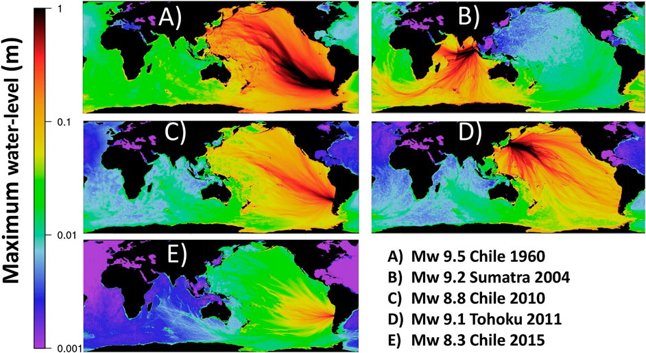
FIGURE 1. Tsunami events considered in this study. The images are model outputs derived using the solver from Section 2.4.3 on the global grid and a subset of the source models in Figure 2 [(A): H19, (B): F07, (C): L11, (D): Y18, (H): W17].

FIGURE 2

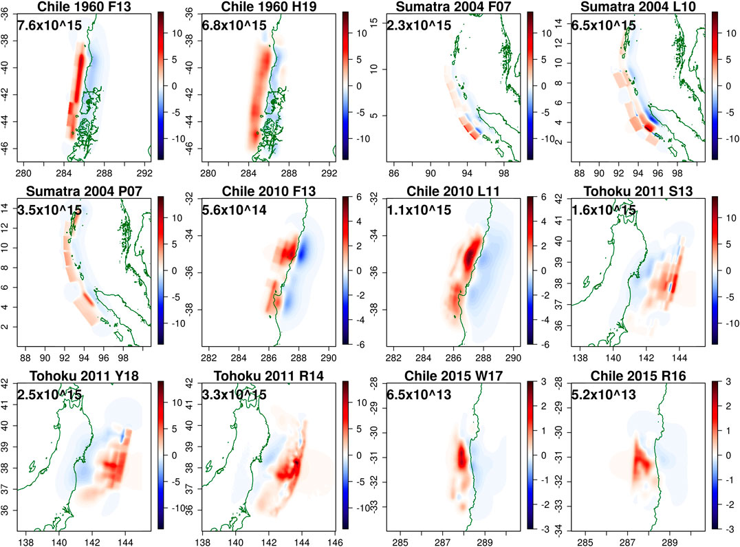
FIGURE 2. The vertical co-seismic displacement for all source models. Text beneath the title gives the initial available potential energy of the ocean surface displacement (kg m²/s², derived by integrating Eq. 5 in space; there is no contribution from deformation on land). The sources are based on finite-fault inversions in the following publications: F13 (Fujii and Satake, 2013); H19 (Ho et al., 2019); F07 (Fujii and Satake, 2007); L10 (Lorito et al., 2010); P07 (Piatanesi and Lorito, 2007); L11 (Lorito et al., 2011); S13 (Satake et al., 2013); Y18 (Yamazaki et al., 2018); R14 (Romano et al., 2014); W17 (Williamson et al., 2017); R16 (Romano et al., 2016).

Most tsunami initial conditions in Figure 2 were derived by computing the vertical co-seismic deformation from the published fault-geometries and slip vectors, assuming instantaneous rupture in a homogeneous elastic half-space (Okada, 1985; Meade, 2007). The effect of horizontal deformation over a sloping seabed (Tanioka and Satake, 1996) was not included as this tends to add shorter waves to the source which may not be well simulated with our long-wave hydrodynamic model (Saito et al., 2014). However source R14 was taken directly from the finite-element model of Romano et al. (2014); this includes horizontal components so is rougher than our other sources (Figure 2). Source H19 was derived from water-surface unit-sources following Ho et al. (2019). A Kajiura filter (Kajiura, 1963; Glimsdal et al., 2013) was applied to all models except the water-surface inversion H19.

The studies on which our source models are based generally inverted the source using deep sea and/or coastal tsunami data, sometimes combined with geodetic data (GPS, InSAR, leveling) and occasionally teleseismic data. None made use of the Australian tide-gauge data studied herein. All inverted the source with linear combinations of earthquake and/or tsunami Green’s functions, in some cases including regularization constraints (L11, Y14, R16, W17, Y18). Most simulated the co-seismic displacement assuming a homogeneous elastic half-space, although R14 used a 3D finite-element model to account for material heterogeneity. Tsunami Green’s functions were mostly modeled with shallow water schemes, although R14, R16 and Y18 employed a non-hydrostatic model. Some papers reported both a best-fitting source model and an average source model; in such cases we always used the former. Full details are available in the repository (see Data Availability Statement).

2.2.Test Sites and Data

The model is compared with data at 16 sites in Australia that have good bathymetry and relatively good quality tsunami observations at tide-gauges (Figure 3). Most gauges only record one of the modeled tsunami events, although Fort Denison in Sydney Harbor records all five (Figure 3). By using multiple sites with good quality data for each historic tsunami, we reduce the risk that site-specific factors limiting the model performance are mistakenly attributed to source/propagation model biases (e.g., undiagnosed errors in the bathymetry or tide-gauge records). No gauge observations were rejected on the basis of disagreement with our tsunami model, to avoid biasing the results.

FIGURE 3

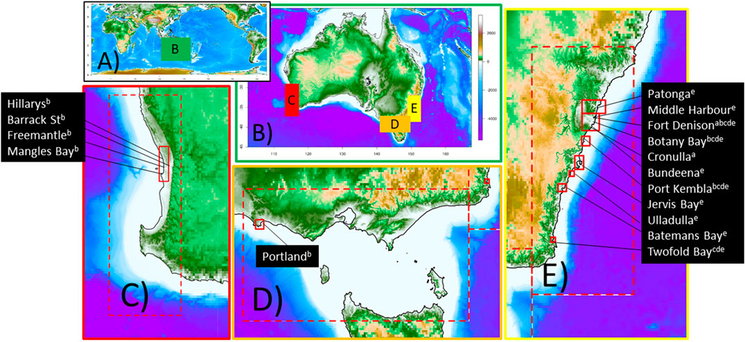
FIGURE 3. The model extent and tide-gauge locations. Superscripts on tide-gauges (a,b,c,d,e) indicate the tsunamis for which we have data, corresponding to the 1960, 2004, 2010, 2011, 2015 events, respectively. (A) The global grid has a spatial resolution of 1-arc-minute and is modeled with reduced-physics approaches; (B) zoom near Australia which shows the three regions where refined grids are used and the NSWE are solved; (C–E) the refined grids around western and south-eastern Australia. Dashed boxes denote regions with 1/7-arc-minute spatial resolution ($\simeq$260 m), and solid boxes denote regions with 1/49-arc-minute resolution ($\simeq$ 37 m) which contain the tide-gauges.

Tide-gauge data was obtained from a range of sources (see Acknowledgments). To detide the observations we first subtracted tidal predictions, which were either provided with the tide-gauge data, or obtained from TPXO7.2 (Egbert and Erofeeva, 2002). Next a high pass filter was used to remove the residual long-period sea-level variations by applying a discrete Fourier transform and zeroing the amplitude of waves with period exceeding a threshold. At most sites the tides are semi-diurnal and the high pass filter threshold was 3 h. At our Western Australia sites the tides are diurnal and a longer threshold was used (6 h); the 3 h threshold led to non-stationary oscillations in the non-tsunami sea-level component at the time of the Sumatra 2004 tsunami, suggesting a longer threshold is appropriate. Irrespective this has little impact on the tsunami signal. In all cases the detided tsunami record might still be affected by other physical processes (e.g., seiching due to transient atmospheric forcings) or measurement errors (e.g., excess mechanical smoothing in the gauge, Satake et al., 1988); however it represents our best estimate of the tsunami signal.

Most gauges used herein have a sampling frequency of 1-min. For the Sumatra 2004 event, three of the four gauges used in Western Australia have 5-min sampling frequency (excepting Hillarys which has a 1-min frequency). For the 1960 Chile event only two gauges are available (Fort Denison and Cronulla), both of which were digitized at approximately 2-min sampling frequency from scans of the analogue tide-gauge records (the former by Wilson et al., 2018). Although in recent decades additional 15-min tide-gauge data is available at several sites, this was not used because it under-samples the tsunami making interpretation more difficult (Rabinovich et al., 2011). At Port Kembla the outer-harbour gauge is used; the inner-harbour gauge was not used based on advice from the data custodians (NSW Port Authority, personal communication 2020) and the issues noted in Allen and Greenslade (2016).

2.3.Tsunami Model

The tsunami is simulated from source to the tide-gauges using the open-source hydrodynamic model SWALS, which solves several variants of the shallow water equations in spherical or Cartesian coordinates and was used for the 2018 Australian Probabilistic Tsunami Hazard Assessment (Davies and Griffin, 2018). The source code includes a validation test-suite of more than 20 analytical, laboratory and field problems, including well-known tests such as those in NTHMP (2012) (excluding landslides) and two recent field-scale NTHMP problems (Macías et al., 2020). It uses structured grids with two-way nesting, and flux-correction to enforce conservation at nested grid boundaries. Different grids can employ different solvers simultaneously; this is used in the current study to test a range of reduced-physics solvers on the global grid (only) while solving the NSWE on refined grids.

The global scale tsunami propagation is simulated on a 1 arc-minute grid (Figure 3A) using bathymetry derived from GEBCO 2014 (Weatherall et al., 2015) and GA250 (Whiteway, 2009) (details in Davies and Griffin, 2018). East-West periodic boundary conditions are used. The southern boundary (79° S) is covered by land. At the northern boundary (68° N) a reflective wall is imposed; while artificial this closes the model and facilitates energy conservation calculations (as SWALS does not track energy fluxes through boundaries). Physically this is reasonable given little tsunami energy will radiate through either Bering strait (which is small) or north Atlantic (which is very far from our tsunami sources). The reduced-physics solvers used on this grid are described in Sections 2.4.2–2.4.4.

Nearshore regions containing good-quality tide-gauge observations are simulated on refined grids (1/7 and 1/49 arc-minutes, (Figures 3C–E), which are linked with the global grid and each other via two-way nesting. Good quality nearshore elevation data is used on the highest-resolution grids, mostly derived from LIDAR and gap-filled using available single-beam bathymetric surveys and gridded elevation from prior studies (see Acknowledgments; Allen and Greenslade, 2016; Wilson and Power, 2018). Breakwalls close to our tide-gauges were burned into the model’s elevation to ensure they are represented irrespective of the grid resolution. On these nearshore grids the tsunami is simulated using the NSWE with Manning-friction (Section 2.4.1).

To check the numerical convergence of the model at the default resolution (1, 1/7 and 1/49 arc-minute nested grids), higher resolution simulations (1/2, 1/14, 1/98 arc-minute) were run for two of our sources (F07, Y18), using the reduced physics solver of Section 2.4.3 on the coarsest grid. Results were compared with the default model at twelve sites with corresponding good-quality observations, as this is where the model results will be used. Waveforms were similar although not completely convergent, with tsunami maxima showing changes ranging from −12% to +21% with a median of 2% (typical examples in Figure 4). In general greater differences are anticipated between the models and data, so the default resolution was considered adequate for the current study.

FIGURE 4

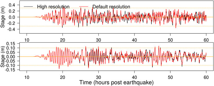
FIGURE 4. Comparison of nearshore gauge results in two models; one with default resolution (1, 1/7, 1/49 arc-minute nested grids) and one with higher-resolution (1/2, 1/14, 1/98 arc-minute nested grids). Locations correspond to tide-gauges at Port Kembla (top) and Botany Bay (bottom); results elsewhere were qualitatively similar. The simulation corresponds to the Tohoku 2011 Y18 source, using Manning-friction in the global model.

2.4.Hydrodynamic Simplifications for Global Scale Tsunami Propagation

Several reduced-physics solvers are tested on the global grid, all based on the linear shallow water equations (LSWE) with alternative dissipation models:

(1) Frictionless (Section 2.4.2)

(2) Nonlinear Manning-friction (Section 2.4.3)

(3) Constant linear-friction (Section 2.4.4)

These represent computationally efficient alternatives to solving the full NSWE for global tsunami propagation.

The frictionless LSWE were tested because they are often used to simulate large-scale tsunami propagation (e.g., Choi et al., 2003; Burbidge et al., 2008; Thio, 2015; Li et al., 2016; Davies and Griffin, 2020) and arguably represent the simplest model of this kind. The Manning-friction approach was tested because it is closer to the full NSWE; however over timescales where dissipation is important, the nonlinearity will prevent a unit-source implementation. The constant linear-friction approach (Fine et al., 2013; Kulikov et al., 2014) was tested because it enables dissipation to be included in a linear framework, with all the associated efficiency benefits. Furthermore, although unit-sources are not employed in this study, below it is shown that solutions of the constant linear-friction model can be well approximated with a simple transformation of solutions of the frictionless LSWE, which is convenient because the latter are available in several existing tsunami propagation databases (e.g., Thio, 2015; Li et al., 2016; Davies and Griffin, 2018).

2.4.1.Nonlinear Shallow Water Equations

The 2D NSWE with friction are (e.g., Baba et al., 2015; Behrens and Dias, 2015):

$\begin{array}{l}\frac{\partial \eta }{\partial t}+\nabla \cdot \mathbf{q}=0\\ \frac{\partial \mathbf{q}}{\partial t}+\nabla \cdot \left(\mathbf{u}\otimes \mathbf{q}\right)+gh\nabla \eta +gh{\mathbf{S}}_{\mathbf{f}}+\mathbf{\Omega }=0\end{array}(2)$

Here $\eta =h+z$ is the free surface elevation (m), h is the depth (m), z is the bed elevation (m), $\mathbf{q}=h\mathbf{u}$ is the 2D flux vector (m²/s), $\mathbf{u}=\left(u,v\right)$ is the 2D velocity vector (m/s), g is gravity (m/s²), ${\mathbf{S}}_{\mathbf{f}}=n^2\mathbf{u}\left|\mathbf{u}\right|h^{-4/3}$ is the friction slope vector with Manning-friction coefficient n, and $\mathbf{\Omega }=\omega \left(-vh,uh\right)$ is the Coriolis force with latitude dependent Coriolis parameter ω.

If friction is neglected (${\mathbf{S}}_{\mathbf{f}}=0$) then for smooth flows Eq. 2 is energy conservative (Arakawa and Hsu, 1990):

${\displaystyle {\int }_D\left(e_k+e_p\right)dA=E_0}(3)$

Here the depth-integrated energy density $\left(e_k+e_p\right)$ is integrated over a two-dimensional domain D with no inflow or outflow through boundaries, $dA$ is an area element, $E_0$ is the constant total energy in D, $e_k$ is the depth-integrated kinetic energy density:

$e_k=\frac{\rho h}{2}\left(u^2+v^2\right)(4)$

with water density ρ (kg/m³), and $e_p$ is the “depth-integrated available potential energy density”:

$e_p=\frac{\rho g}{2}\left({\eta }^2-z^2\right)+C_2(5)$

By definition the integral of $e_p$ in D is zero if the fluid mass is redistributed in D to make the free-surface constant (Lorenz, 1955); herein $C_2$ is a constant that satisfies this definition. If the vertical datum is the model’s mean sea level, and there is no wetting and drying, then Eq. 5 simplifies to $e_p=\frac{\rho g}{2}{\eta }^2$ in wet regions and zero in dry regions. The latter form is common in the tsunami literature (Tang et al., 2012; Saito et al., 2014; Tolkova, 2014) but does not generalize to flows with wetting and drying or other vertical datums.

On refined grids the model herein solves Eq. 2 in flux-conservative form with a constant Manning-friction $n=0.03$. The refined-grid n value might be improved with site-specific tuning, but that was not attempted herein. A second-order accurate finite-volume scheme is used based on the hydrostatic-reconstruction approach of Audusse et al. (2004). The details are similar to the ANUGA software’s DE1 flow algorithm (Davies and Roberts, 2015), although the latter uses a triangular mesh while the solver herein uses structured grids with two-way nesting.

2.4.2.Linear Shallow Water Equations Without Friction

In the deep ocean even large earthquake tsunamis are of small amplitude relative to ocean depths and velocities are slight compared to the gravity wave speed. Under these conditions Eq. 2 is well approximated with the frictionless LSWE:

$\begin{array}{l}\frac{\partial \eta }{\partial t}+\nabla \cdot \mathbf{q}=0\\ \frac{\partial \mathbf{q}}{\partial t}+g{h}_0\nabla \eta +g{h}_0{\mathbf{S}}_{0\mathbf{f}}+\mathbf{\Omega }=0\end{array}(6)$

Here $h_0$ is the time-invariant depth below mean-sea-level, and the friction slope is zero

${\mathbf{S}}_{0\mathbf{f}}=0(7)$

but is included in Eq. 6 to facilitate extensions below. These equations are also energy conservative.

Herein the LSWE are solved numerically with the classical leap-frog scheme (Goto and Ogawa, 1997). Importantly this scheme has good numerical energy conservation; in our twelve simulations that used the frictionless LSWE on the global grid the numerically integrated energy (Eq. 3) varied within [−2.7%, 0.25%] over 60 h. Minor dissipation is expected in the full model because refined grids solve the NSWE with friction and employ a more dissipative finite-volume numerical scheme; minor energy increase can occur because the leap-frog scheme is not perfectly energy conservative. In comparison the literature suggests global tsunami propagation simulations often have much greater numerical dissipation; Tang et al. (2012) and Tolkova (2014) used several variants of the MOST and CLIFFS solvers to simulate the Tohoku tsunami globally without friction and found $\simeq$ 80–90% of the total energy was numerically dissipated in 24 h. Popinet (2011) reported substantial numerical dissipation when modeling the Sumatra 2004 tsunami from source with the Gerris finite-volume solver. Although the frictionless LSWE are energy conservative, physically some dissipation is expected. Considering the observed energy e-folding timescale of global tsunamis at late-times ($\simeq 1$ day) these frictionless LSWE simulations should under-estimate the physical dissipation, but the numerical scheme offers a good basis for testing dissipation models because it adds negligible numerical dissipation.

2.4.3.Linear Shallow Water Equations With Manning-Friction

To add dissipation to the global model it is natural to consider a Manning-friction closure in Eq. 6. For computational efficiency our approach exploits the approximation $h\simeq h_0$ inherited from the LSWE:

${\mathbf{S}}_{0\mathbf{f}}=\mathbf{q}\left|\mathbf{q}\right|\left(n^2{h}_0^{-10/3}\right)(8)$

where n is the Manning-friction coefficient, which was set to 0.035 on the global grid (slightly larger than our nearshore Manning coefficient of 0.03). Real tsunamis likely dissipate due to a mixture of nonlinear bottom friction in shallow regions, and other deep-ocean dissipation mechanisms which are important for simulating tides (Egbert and Ray, 2000; Buijsman et al., 2015; Kleermaeker et al., 2019). Our global model poorly resolves most shallow nearshore areas, neglects nonlinear tidal interactions, and ignores other dissipation mechanisms, so the Manning model is likely a strong simplification of reality. In preliminary simulations we also tried a smaller global Manning coefficient ($n=0.02$) which did not perform as well; however further optimization of the global n may be possible.

Equation 8 is nonlinear so solutions cannot be constructed from unit-sources (at least not over timescales long enough for nonlinear dissipation to be important). However the term in large parenthesis is time-invariant which reduces the computational expense of our implementation. A semi-implicit discretization is used to include Eq. 8 in the leap-frog scheme, with $\left|\mathbf{q}\right|$ evaluated explicitly and $\mathbf{q}$ evaluated implicitly. The total energy dissipation over 60 h varied between 63 and 96% in our twelve simulations using this model on the global grid, with the lowest percentage dissipation corresponding to the smallest tsunami (2015 Chile) as expected with quadratic friction.

For global tsunami propagation this model is relatively close to the NSWE with Manning-friction (Eq. 2). Figure 5 compares solutions at some nearshore tide-gauges when using the above reduced-physics model on the global grid, vs. the full NSWE (the latter were solved with a leap-frog numerical scheme combined with an upwind treatment of nonlinear advection, for similarity with our reduced-physics solver, Goto and Ogawa, 1997; Liu et al., 1995). At our nearshore gauges of interest, which are inside the refined grids and thus simulated with the NSWE finite-volume scheme (Section 2.4.1), the difference between the two models is smaller than differences caused by grid refinement (compare Figures 4 and 5). However the full simulation ran three times faster when using the simpler model on the global grid (about 2 vs. 6 h for the 60 h simulation with all nested grids, using 8 CPU nodes of the Gadi supercomputer NCI, 2020), due purely to a factor-of-6.6 speedup in the global grid calculation.

FIGURE 5

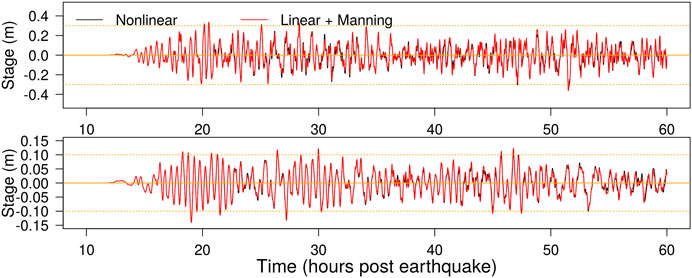
FIGURE 5. Comparison of nearshore gauge results in two models which use different solvers on the global grid; one solves the full NSWE, the other solves the LSWE with a nonlinear Manning-friction term. In both cases the NSWE are solved on refined grids. The site locations and scenario details are the same as in Figure 4.

2.4.4.Linear Shallow Water Equations With Constant Linear-Friction, and Approximation via Frictionless Solutions

To represent global-scale tsunami dissipation with a linear model, Fine et al. (2013) and Kulikov et al. (2014) appended constant linear-friction to the LSWE (Eq. 6) by replacing $\frac{\partial }{\partial t}\to \left(\frac{\partial }{\partial t}+f\right)$ in the momentum equations only, implying:

${\mathbf{S}}_{0\mathbf{f}}=f\mathbf{q}/\left(g{h}_0\right)(9)$

where f is a constant linear drag coefficient. Fine et al. (2013) and Kulikov et al. (2014) show Eqs 6 and 9 cause the globally integrated energy to decay exponentially in time with e-folding timescale of $1/f$, thus mimicking classical observations of tsunami energy time-decay at late times (Miller et al., 1962; Munk, 1963; van Dorn, 1984; van Dorn, 1987; Rabinovich et al., 2011; Rabinovich et al., 2013). On this basis they used $f=1\times {10}^{-5}$ which corresponds to an energy e-folding time of 27.7 h. Herein an implicit discretization is used to include Eq. 9 in the leap-frog scheme for Eq. 6. The total energy dissipation over 60 h was close to 88.5% for all twelve simulations using this model on the global grid, as expected theoretically.

Linear-friction is attractive, if it works well enough in practice, because the model retains all the practical benefits of linearity for simulating global propagation (e.g., unit-source solutions are exact). The use of a constant f is not essential to preserve linearity; often linear friction is implemented by linearizing a quadratic drag model about a reference depth and velocity (e.g., Tolkova, 2015). However the use of a constant f has a practical advantage, above those noted in Fine et al. (2013) and Kulikov et al. (2014): it is possible to approximate solutions of the model with negligible error by using transformed solutions of the frictionless LSWE (Eqs 6 and 7). To illustrate this point, Figure 6 compares a numerically derived solution to the constant linear-friction model Eqs 6 and 9 with an “approximate linear-friction” solution defined as:

$[{\eta }^a,u{h}^a,v{h}^a]=\text{exp}\left(-\frac{f}{2}t\right)[{\eta }^0,u{h}^0,v{h}^0](10)$

Here the superscript a denotes the approximate linear-friction solution, and the superscript 0 denotes the frictionless LSWE solution which is prescribed the same initial conditions as the solution of interest.

FIGURE 6

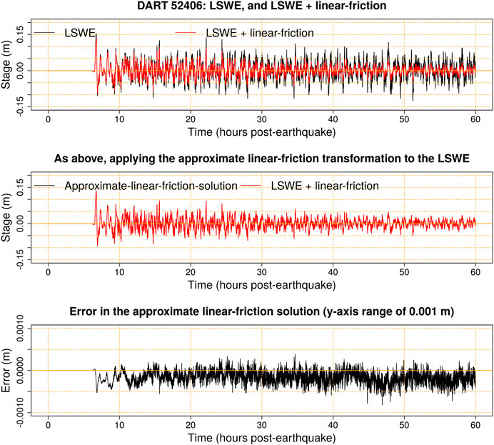
FIGURE 6. Illustration of the approximate linear-friction solution at a deep ocean site (DART 52406), using the Y18 source. Top: Comparison of numerical solutions using the frictionless LSWE (Section 2.4.2) and the LSWE with constant linear-friction (Section 2.4.4). Middle panel: Comparison of the approximate linear-friction solution (derived with the LSWE solution via Eq. 10) and the LSWE with constant linear-friction. They are visually indistinguishable. Bottom: Difference between the two solutions in the middle panel, using a vertical scale of $\pm 0.001$ m.

Although Eq. 10 does not produce an exact solution of the constant linear-friction model, the error is negligible in practice (Figure 6) for global-scale tsunamis and other waves having a period much smaller than the decay timescale $1/f$. This is justified mathematically below. Thus unit-source databases based on the frictionless LSWE can be used, without modification, as a convenient means to derive solutions with linear-friction using Eq. 10. This makes the model very easy to use in practice, via existing frictionless tsunami scenario databases, and motivates us to test it herein.

2.4.4.1Justification of the Approximate Linear-Friction Solution (Eq. 10)

It is standard to convert the frictionless LSWE to a single wave equation for the free surface by applying $\frac{\partial }{\partial t}$ to the mass equation and $\nabla \cdot$ to the momentum equation in Eq. 6, and eliminating mixed derivatives of $\mathbf{q}$. Using the superscript 0 to denote solutions of the frictionless LSWE, this leads to:

$\frac{{\partial }^2{\eta }^0}{\partial t^2}-\nabla \cdot \left(g{h}_0\nabla {\eta }^0\right)-\nabla \cdot {\mathbf{\Omega }}^0=0(11)$

where ${\mathbf{\Omega }}^0=\omega [-v{h}^0,u{h}^0]$. For solutions of the constant linear-friction model (denoted with superscript l) the same calculation yields an additional source-term on the RHS:

$\frac{{\partial }^2{\eta }^l}{\partial t^2}-\nabla \cdot \left(g{h}_0\nabla {\eta }^l\right)-\nabla \cdot {\mathbf{\Omega }}^l=-f\frac{\partial {\eta }^l}{\partial t}(12)$

For the approximate linear-friction solution (Eq. 10), the analogous equation follows by substituting $[{\eta }^0,u{h}^0,v{h}^0]=\text{exp}\left(\frac{f}{2}t\right)[{\eta }^a,u{h}^a,v{h}^a]$ into Eq. 11:

$\frac{{\partial }^2{\eta }^a}{\partial t^2}-\nabla \cdot \left(g{h}_0\nabla {\eta }^a\right)-\nabla \cdot {\mathbf{\Omega }}^a=-f\frac{\partial {\eta }^a}{\partial t}-{\eta }^a\frac{f^2}{4}(13)$

Equation 13 is the same as Eq. 12 except for the second RHS source term, which has magnitude $\simeq \alpha f^2/4$ where α is the wave amplitude. If the wave has period T then the average absolute value of $\frac{\partial {\eta }^a}{\partial t}$ is $4\alpha /T$. Thus the first RHS source-term has magnitude $\simeq f\left(4\alpha /T\right)$, so is $\simeq 1000$ times larger than the second source term for a typical earthquake-generated tsunami in the deep ocean (period 30 min, $f\simeq {10}^{-5}$). In this circumstance Eq. 13 is a minor perturbation of Eq. 12 and their solutions will be arbitrarily close if $fT/16$ is sufficiently small, which explains the excellent agreement in practice (Figure 6).

3.Results

Section 3.1 provides examples to illustrate how the global dissipation models affect nearshore tsunami simulations in comparison with data. This gives context for a subsequent statistical analysis but necessarily represents a small sample of the results; figures comparing models and data at all sites are available via the repository (see Data Availability Statement). Section 3.2 uses statistical techniques to evaluate each model by comparing all simulations and observations simultaneously, focusing on biases in the modeled tsunami maxima and their relation to the simulation duration. These results motivate tests of several modified linear-friction models on the global grid (Section 3.3). Section 3.4 considers how the model performance varies among the source-inversions.

3.1.Effect of Global Dissipation at Nearshore Gauges: Examples

3.1.1.Fort Denison, Chile 1960, H19 Source Model

The 1960 Chile tsunami was observed widely on Australia’s east-coast where it induced widespread marine hazards and minor inundation (Beccari, 2009). Based on our simulations, the tsunami reached the eastern Australian mainland $\simeq$ 14 h after the earthquake via waves which propagated south of New Zealand. Further waves arrived via the ocean north of New Zealand, including due to prominent scattering of the leading wave around bathymetry near French Polynesia ($\simeq$ 11 h post-earthquake, reaching eastern Australia $\simeq 22$ h post-earthquake). This led to a steady growth in the nearshore tsunami energy on Australia’s east coast (Figure 7). At Fort Denison the largest waves occurred around 25–29 h post-earthquake, while they were slightly earlier ($\simeq 22-25$ h) at the Cronulla gauge which is 25 km south and closer to the open coast.

FIGURE 7

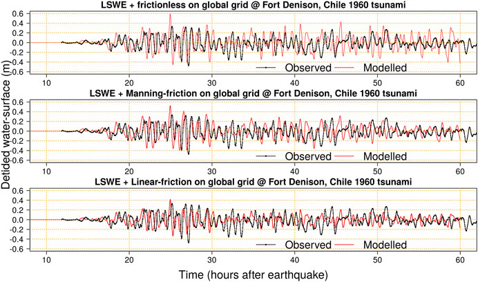
FIGURE 7. Simulations and observations of the Chile 1960 tsunami at Fort Denison near Sydney. All simulations use the Chile 1960 H19 source model. Top: Using the frictionless LSWE on the global grid. Middle: Using LSWE with Manning-friction on the global grid. Bottom: Using LSWE with linear-friction on the global grid.

At Fort Denison the models with frictionless and Manning-friction global grid solvers give similar results prior to the observed maxima, with predicted waves slightly larger than observed (Figure 7). Linear-friction on the global grid produces slightly smaller initial waves. Constant linear-friction induces greater dissipation in the deep-ocean compared to Manning-friction which dissipates most energy in nearshore areas; at later times the cumulative effect of nearshore propagation leads to significant global energy dissipation with Manning-friction, but this has little influence on the early arrivals. All models well approximate the timing of the maximum wave but differ in its size (Figure 7). In this case linear-friction best represents the observed tsunami maxima, but at later times consistently under-predicts the tsunami size. Manning-friction better simulates the size of late arriving waves, while the frictionless global model leads to nearshore waves that are too large at late times.

The data has a phase-lag relative to all models (Figure 7). This is expected given our use of the LSWE on the global grid. The phase-lag should be better simulated by including additional terms in the global model related to loading, seawater density stratification, and self-gravitation (Watada et al., 2014; An and Liu, 2016), although this would be computationally expensive (Allgeyer and Cummins, 2014; Baba et al., 2017).

3.1.2.Hillarys, Sumatra 2004, F07 Source Model

The Sumatra 2004 tsunami induced significant marine hazards in Western Australia, including 35 ocean rescues, damages to boats and marinas, and minor inundation at a number of coastal towns (Anderson, 2015). It took about 6 h to reach Hillarys in Western Australia (Figure 8), which is the shortest travel time among the tsunamis considered herein. The fourth wave was the largest at Hillarys and occurred a few hours after the tsunami arrival, although waves around 21 h post-earthquake were only slightly smaller (Figure 8). Pattiaratchi and Wijeratne (2009) noted these later waves were the largest observed at several other sites in Western Australian, and attributed them to tsunami energy reaching Australia via reflections off distant Indian Ocean topography.

FIGURE 8

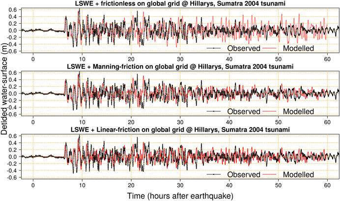
FIGURE 8. Simulations and observations of the Sumatra 2004 tsunami at Hillarys in Western Australia. All simulations use the Sumatra 2004 F07 source model. Top: Using the frictionless LSWE on the global grid. Middle: Using LSWE with Manning-friction on the global grid. Bottom: Using LSWE with linear-friction on the global grid.

At Hillarys the simulated leading waves are not strongly affected by the choice of global dissipation model (Figure 8). About 30 h post-earthquake the frictionless global model results in larger nearshore waves than simulations with friction, although initially it is not obvious that any model better agrees with data. However from about 36 h post-earthquake the frictionless global model consistently predicts larger nearshore waves than were observed, as seen in the previous Chile 1960 example, indicating a lack of global dissipation. At late times the models with global friction predict smaller waves and agree much better with data in the nearshore (Figure 8).

The data evidences some phase-lag relative to the model, as noted in the previous Chile 1960 example. For instance the modeled long-period wave around 20–23 h arrives slightly earlier than the observed wave (Figure 8), and a similar result is obtained with the P07 and L10 source models (see online repository). These phase-lags may be better modeled by accounting for loading, seawater density stratification, and self-gravitation (Baba et al., 2017). The neglect of wave dispersion is also likely to be significant for the Sumatra 2004 example, which shows much more short-period wave energy than the Chile 1960 example (e.g., compare Figures 7 and 8). Non-dispersive shallow-water wave theory will over-estimate the celerity of shorter period waves, as previously noted in the context of the 2004 Sumatra tsunami (Kulikov, 2006).

3.1.3.Twofold Bay, Tohoku 2011, S13 Source Model

The 2011 Tohoku tsunami was widely observed in eastern Australia (Hinwood and Mclean, 2013). The initial waves reached Australia’s east-coast via straits around eastern Papua New Guinea, the Solomon Islands and Vanuatu, while at later times much of the wave energy arrived via the ocean north of New Zealand (Hinwood and Mclean, 2013). Our models suggest the leading wave reached South America around 20–22 h post-earthquake where it was prominently reflected into the Pacific Ocean, adding significantly to the late-time wave energy in the southwest Pacific Ocean. In eastern Australia the tide-gauges at Fort Denison and Twofold Bay exhibited late-time maxima (46–50 h post-earthquake, Figure 9) while gauges at Botany Bay and Port Kembla exhibited earlier maxima (18–20 h post-earthquake) but nonetheless showed relatively large late-time waves that we attribute to reflections from the eastern Pacific. This is similar to reports from New Zealand where Borrero et al. (2015a) found some sites (but not all) experienced late-time tsunami maxima up to 2 days post-earthquake.

FIGURE 9

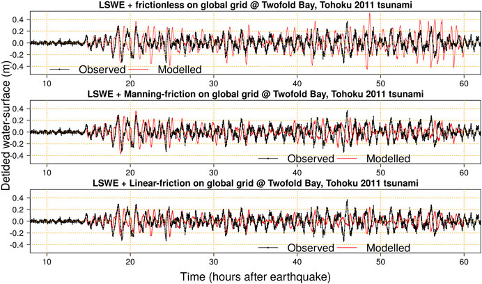
FIGURE 9. Simulations and observations of the Tohoku 2011 tsunami at Twofold Bay. Note the observed late-time maxima 46 h post-earthquake. All simulations use the Tohoku 2011 S13 source model. Top: Using the frictionless LSWE on the global grid. Middle: Using LSWE with Manning-friction on the global grid. Bottom: Using LSWE with linear-friction on the global grid.

At Twofold Bay the first few waves (up to 20 h post-earthquake) are similar in the models with frictionless and Manning-friction global grid solvers, and agree quite well with data (Figure 9). Linear-friction produces smaller initial waves than the Manning model, as noted for above for the Chile 1960 tsunami, which is attributed to its greater dissipation in the deep ocean. At late times the frictionless global model produces overly large waves in the nearshore compared to data (as in the previous examples). In this case the Manning and linear-friction models predict late-time waves smaller than were observed. These results again highlight the sensitivity of later waves to the global dissipation model.

3.2.Effect of Global Dissipation at Nearshore Gauges: Tsunami Maxima Statistics

To compare the models and observations at all gauges simultaneously the tsunami maxima (i.e. detided water-level maxima) is used following Allen and Greenslade (2016) and Adams and LeVeque (2017). The results above suggest that model biases may be related to the simulation duration, and to assess this both simulations and data are truncated to various time-intervals (Figure 10):

(1) 0–8 h after the tsunami arrival. The arrival time is defined, for each model and gauge separately, as the time that the modeled stage absolute value exceeds $5\times {10}^{-4}$ of its maximum, and is typically 12 h post-earthquake herein (range of 5.8–16.0 h).

(2) 0–36 h post-earthquake.

(3) 0–60 h post-earthquake.

(4) The last day of the 60 h simulation (i.e., 36–60 h post-earthquake).

FIGURE 10

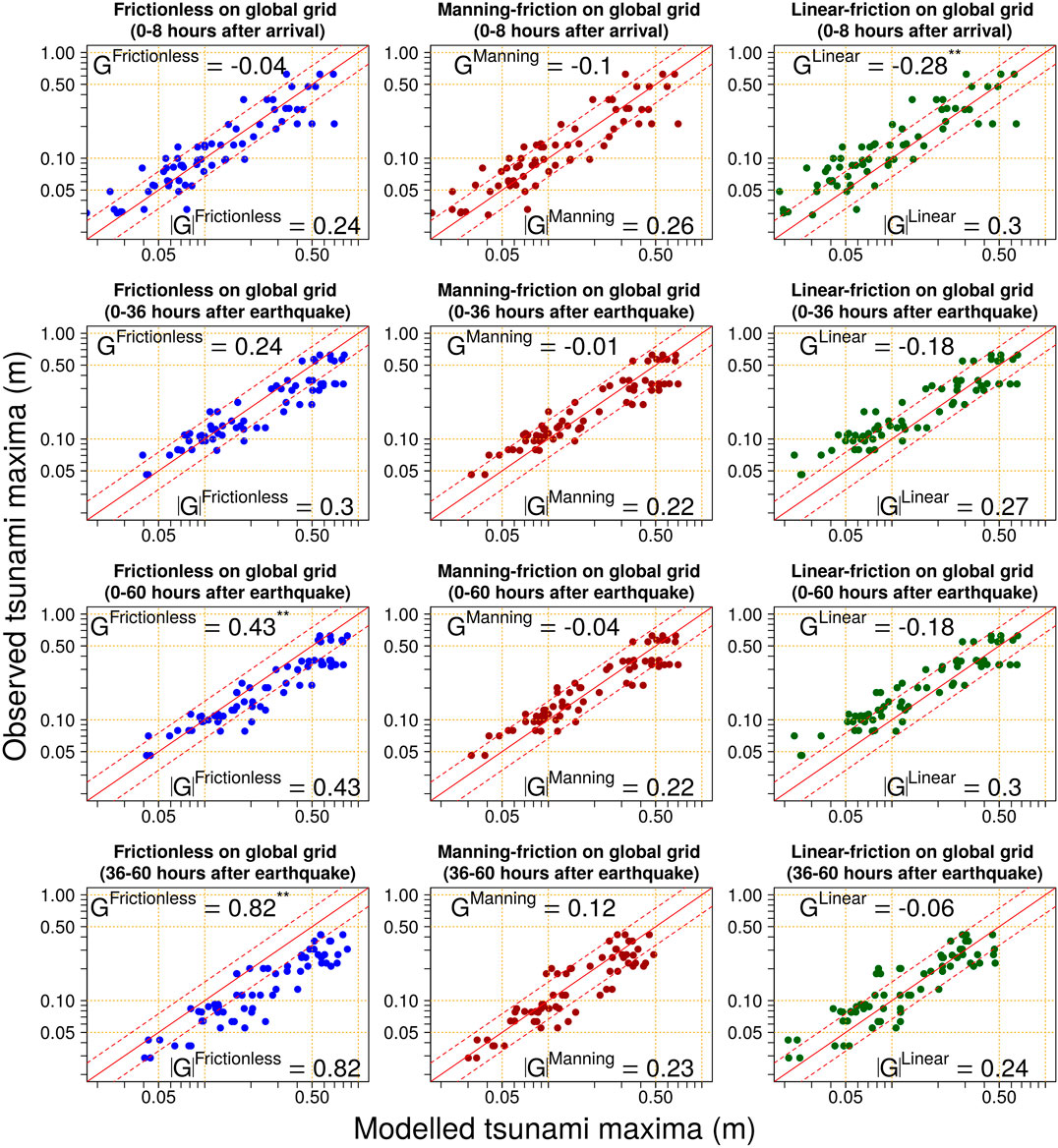
FIGURE 10. Modelled-vs-observed tsunami maxima for different global model types (frictionless, Manning-friction, linear-friction), and different temporal subsets of the simulation (0–8 h after tsunami arrival; 0–36 h after earthquake; 0–60 h after earthquake, 36–60 h after earthquake). Diagonal solid line is $y=x$; diagonal dashed lines are $y=1.5x$ and $y=x/1.5$. Where the $G_m$ values are followed by $\text{**}$, there were 10 or more source-inversions having $G_i^m$ values of the same sign.

All but one observed time-series extends for the full 60 h simulation; the 1960 Cronulla tide-gauge record is truncated at 29 h post-earthquake and dropped from comparison with longer simulations.

Statistics describing the model bias ($G^m$) and accuracy ($|G{|}^m$) are reported for each variation of the global model $m\in \left(\text{Frictionless},\text{ Manning},\text{ Linear}\right)$ (Figure 10). These emphasize the error as a fraction of the observation and deliberately weight each source inversion equally, even though they have different numbers of corresponding gauge observations, because biases in any one source-inversion will lead to correlated errors among its gauges (Section 3.4).

The bias statistic $G^m$ summarizes the relative model bias (e.g., $G^m=-0.1$ suggests 10% under-estimation is typical). It is calculated as:

$\begin{array}{l}{G}^m=\underset{i\in \text{source inversions}}{\text{Median}}\left(G_i^m\right)\\ G_i^m=\underset{j\in \text{available gauge observations for source inversion }i}{\text{Median}}\left(\left(p_{i,j}^m-d_j\right)/d_j\right)\end{array}(14)$

Here $G_i^m$ gives the median relative error for model m and source-inversion i ($i=1\dots 12$) over all available tide-gauges j. The tide-gauges have observed tsunami maxima $d_j$ and modeled tsunami maxima $p_{i,j}^m$.

The superscript“**” is appended to $G^m$ values that show strong evidence of being significantly different from zero. It is applied when 10 or more of the 12 $G_i^m$ values have the same sign. This criterion is heuristic but is motivated by the following argument: if the model m and source-inversions i have little bias on average then any $G_i^m$ has an equal chance of being positive or negative. If all $G_i^m$ are independent then the signs of the $G_i^m$ behave like a binomial random variable, and with 12 source models the resulting binomial distribution (parameters $p=0.5,\text{size}=12$) implies a 96% chance that fewer than 10 have the same sign.

The accuracy statistic $|G{|}^m$ is similar to $G^m$, except the absolute value of the relative model error is used:

$\begin{array}{l}|G{|}^m=\underset{i\in \text{source inversions}}{\text{Median}}\left(|G{|}_i^m\right)\\ |G{|}_i^m=\underset{j\in \text{available gauge observations for source inversion }i}{\text{Median}}\left(|\left(p_{i,j}^m-d_j\right)/d_j|\right)\end{array}(15)$

Thus $|G{|}^m$ estimates the typical magnitude of the model error as a fraction of the data, irrespective of its sign.

Figure 10 highlights the interaction of the simulation duration and the model bias, most prominently for the frictionless global model. If simulations are restricted to 0–8 h following tsunami arrival, this model exhibits small bias and a typical accuracy around 24% (top-left panel of Figure 10). For a 36 h simulation there is increasing positive bias ($\simeq 24\text{\%}$), which becomes pronounced in the 60 h simulation ($\simeq 43$%). The frictionless model bias on the last day of 60 h simulation is very strong ($\simeq 82$%), emphasizing that it consistently overestimates the size of late-arriving waves (Section 3.1).

Manning-friction in the global model leads to much better agreement with observed tsunami-maxima for long simulations (Figure 10). For short simulations (0–8 h post-arrival) it performs similarly to the frictionless model, suggesting friction has limited influence on early arriving waves. But over long simulations the cumulative effect of nearshore dissipation at the global scale reduces the nearshore wave heights, in a manner broadly consistent with observations (Figure 10).

Linear-friction in the global model induces a moderate negative bias in the early (0–8 h post-arrival) nearshore tsunami maxima ($\simeq -28\%**$, Figure 10). The constant linear-friction formulation induces greater deep-ocean dissipation than Manning-friction, and the results here suggest this dissipation is too large. However the bias weakens for longer simulations, and for the final 36–60 h post-earthquake the model performs as well as Manning-friction (Figure 10). Compared with the frictionless model, which shares the advantages of linearity, the constant linear-friction model is clearly superior at late times but inferior at short times (Figure 10).

To gauge the model accuracy it is useful to cross-reference the $G^m$ and $|G{|}^m$ statistics in Figure 10 with previous studies which compared modeled and observed tsunami maxima for multiple source-inversions. Allen and Greenslade (2016) modeled 9 historic tsunamis at Port Kembla outer-harbour with the MOST model, using source inversions based on the T2 database (Greenslade et al., 2011). From data in table 3 of Allen and Greenslade (2016) we computed $G^m=-0.1$ and $|G{|}^m=0.36$. Their results at another inner-harbour site were less accurate but are not reported herein because the tide-gauge accuracy is doubtful (NSW Port Authority, personal communication 2020). Adams and LeVeque (2017) studied five source-inversions with 4–6 gauges each using two models (GEOCLAW and MOST). Using results tabulated in Figure 3 of Adams and LeVeque (2017) we compute $G^m=-0.11,-0.01$ and $|G{|}^m=0.375,0.213$, respectively. Given the small number of source-inversions and gauges used in all studies, and their different methodologies, differences between these statistics are probably not meaningful. But they suggest model errors comparable to those obtained with our methodology using global-scale Manning-friction (at all times); using the global-scale frictionless model (at early times); and using global-scale linear-friction (at late times).

3.3.Alternative Linear-Friction Models With Reduced Bias for Earlier Waves

Because linear models have significant practical benefits (e.g., unit sources), herein two variations of the linear-friction model are tested. Both aim to reduce downward bias in nearshore waves 0–8 h after arrival, as compared with the constant linear-friction model, while retaining the benefits of friction for longer simulations. In addition, both models retain the convenient property that their solutions can be approximated from solutions of the frictionless model:

(1) Reduced-linear-friction. This model uses $f=1/\left(36\times 3600\right)\simeq 7.71\times {10}^{-6}$, corresponding to an artificially long tsunami energy e-folding timescale of 36 h (vs. 27.7 h in the original model). The 36 h decay-timescale will reduce energy loss but is a-priori expected to be too long, noting Rabinovich et al. (2013) empirically estimated energy-decay timescales less than 36 h (more typically 24 h) at all DART buoys which recorded the 2009 Samoa, 2010 Chile, and 2011 Tohoku tsunamis.

(2) Delayed-linear-friction. This model is frictionless for the first 12 h, and subsequently uses $f=1\times {10}^{-5}$ as for the original linear-friction model. The heuristic motivation for an initial frictionless period is that early waves reach Australia predominantly via the deep-ocean, with few nearshore interactions, so the cumulative effect of bottom friction should initially be small. The 12 h time-period matches the median tsunami arrival time for the events studied herein (Section 4 will consider alternative estimates of this time-period). In contrast to reduced-linear friction, this model’s late-time energy-decay timescale remains broadly consistent with observations (Rabinovich et al., 2013). Solutions of this model can still be well approximated by frictionless solutions via straightforward modification of Eq. 10:

$[{\eta }^a,u{h}^a,v{h}^a]=\text{exp}\left(-\frac{f}{2}\text{Max}\left(0,t-t_{12}\right)\right)[{\eta }^0,u{h}^0,v{h}^0](16)$

where $t_{12}$ gives the number of seconds in 12 h. Figure 11 compares the performance of these models and the original linear-friction model with data.

FIGURE 11

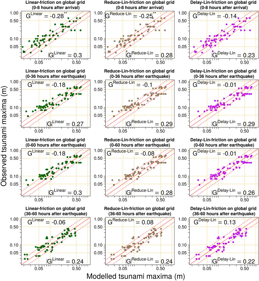
FIGURE 11. Modelled-vs-observed tsunami maxima for different global model types (linear-friction, linear-friction with a lower friction factor, linear-friction with delayed onset of 12 h), and different temporal subsets of the simulation (0–8 h after tsunami arrival; 0–36 h after earthquake; 0–60 h after earthquake, 36–60 h after earthquake). Diagonal solid line is $y=x$; diagonal dashed lines are $y=1.5x$ and $y=x/1.5$. The LHS column is the same as in Figure 10.

The reduced-linear-friction model continues to show downward bias for waves 0–8 h after arrival, even though its friction coefficient is a-priori too small (Figure 11). If constant linear-friction were a good approximation of dissipation for early-arriving waves, then the a-priori small friction coefficient should lead to overestimation of tsunami maxima, but this does not occur. That indicates weaknesses in the constant linear-friction parameterization of tsunami dissipation; friction is still too large in the deep ocean. However the model performs reasonably well for longer simulations (Figure 11).

In contrast, the delayed-linear-friction model performs better in the 0–8 h post-arrival period than any other linear model with friction (Figure 11). Furthermore, over longer simulations it continues to exhibit relatively low-bias in the tsunami maxima, with results comparable to the Manning-friction model (Figure 10). Among the linear models tested herein, this appears the most promising overall for simulating global-scale tsunami propagation.

3.4.Source-Inversion Effects on Modeled Tsunami Maxima

The previous section highlights that error in the modeled tsunami maxima varies from gauge-to-gauge and also depends on the simulation duration. However there is also a significant component related to the source-inversion itself (Figure 12). For simplicity Figure 12 only depicts results using the Manning-friction and delayed-linear-friction global models, which exhibited the least overall bias above, although comparable variations between source-inversions exist for the other models.

FIGURE 12

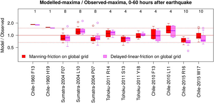
FIGURE 12. Per-inversions boxplots of ratio between modeled and observed tsunami maxima at all gauges, for simulations of 60 h, and two model types. The integers above the boxes count the tide-gauge observations. Dotted horizontal lines are $y=1.5$ and $y=1/1.5$. Definition of the boxplots: The box defines the inter-quartile range with the central line defining the median. The “whiskers” extend from the box for at most 1.5 inter-quartile ranges, or up to the range of the data. Points not covered by whiskers are plotted directly. The Chile 1960 sources only have one gauge record that covers the 0–60 h simulation (Figure 7), so the boxplot reduces to a horizontal line.

For a given historical tsunami, inversions with a larger model/observed ratio in Figure 12 tend to have greater available potential energy in their ocean-displacement (reported in Figure 2). For example consider the Chile 2010 tsunami; the L11 inversion produces higher model/obs ratios than the F13 inversion, while the former also exhibits greater available potential energy (Figures 2, 12). For the Chile 2015 tsunami the W17 inversion exhibits greater model/obs than the R16 inversion, and has greater initial available potential energy (Figures 2, 12). Other cases behave similarly with one exception; for Sumatra 2004 the P07 inversion has slightly smaller model/observed than the F07 inversion (Figure 12), despite having a slightly larger available potential energy (Figure 2). This may reflect that compared to F07, the P07 inversion has greater co-seismic displacement toward the north of the rupture area (Figure 2), which may have less effect on Australia than deformation in the southeast due to tsunami dynamics in the Bay of Bengal. In any case this result is consistent with the suggestion of Titov et al. (2016) that far-field tsunamis are sensitive to the location and energy of the initial ocean-surface displacement, with other source details having a secondary role.

4.Discussion

Linear models provide a very convenient basis for global-scale tsunami scenario databases, and these are often implemented without friction (Burbidge et al., 2008; Li et al., 2016; Davies and Griffin, 2020). Our results suggest this approach is adequate for simulating tsunami maxima up to 8 h following tsunami arrival, when combined with nearshore models based on the NSWE with Manning-friction. Herein 8 h post-arrival corresponds to a median of 20 h post-earthquake; for hazard applications this duration would typically include the most significant waves for the most hazardous scenarios, where sites of interest are well exposed to the tsunami’s leading wave. However, tsunamis may remain dangerous for a considerably longer duration. Over longer simulations the lack of global model dissipation leads to slow divergence of the frictionless model wave heights, as compared to both data and models with friction. It is difficult to estimate a “threshold” duration after which the frictionless model biases become important. In comparison to observed tsunami maxima, our results for 36 h simulations suggest bias $\simeq 24\text{\%}$ in the frictionless model, but considering variations among the source-inversions this is not strong enough to be conclusive. However the biases are very clear in frictionless simulations of 60 h duration, especially if the model-data comparison is restricted to final 36–60 h post-earthquake.

The late-time model biases are largely removed using nonlinear Manning-friction in the global propagation model with $n=0.035$. For simulations of 24 h duration the resulting tsunami maxima are often $\simeq$ 10% smaller than with the frictionless model, but the difference grows for longer simulations (top row of Figure 13). Because Manning-friction is nonlinear this approach cannot be applied using unit-sources (at least not over timescales long enough for nonlinear-dissipation to be important), but it is a good option if one can simulate the tsunami from source. From a physical perspective this model remains over-simplified; it neglects tides which will interact nonlinearly with the tsunami, and furthermore, the tidal literature suggests about one-third of tidal-dissipation occurs in the deep ocean due to mechanisms that are not represented with shallow-water bottom friction (Egbert and Ray, 2000; Buijsman et al., 2015). However we focus on pragmatic methodologies for applications, and by this standard Manning-friction is a good choice for late-time global-propagation simulation, assuming it is viable to model tsunami propagation from source.

FIGURE 13

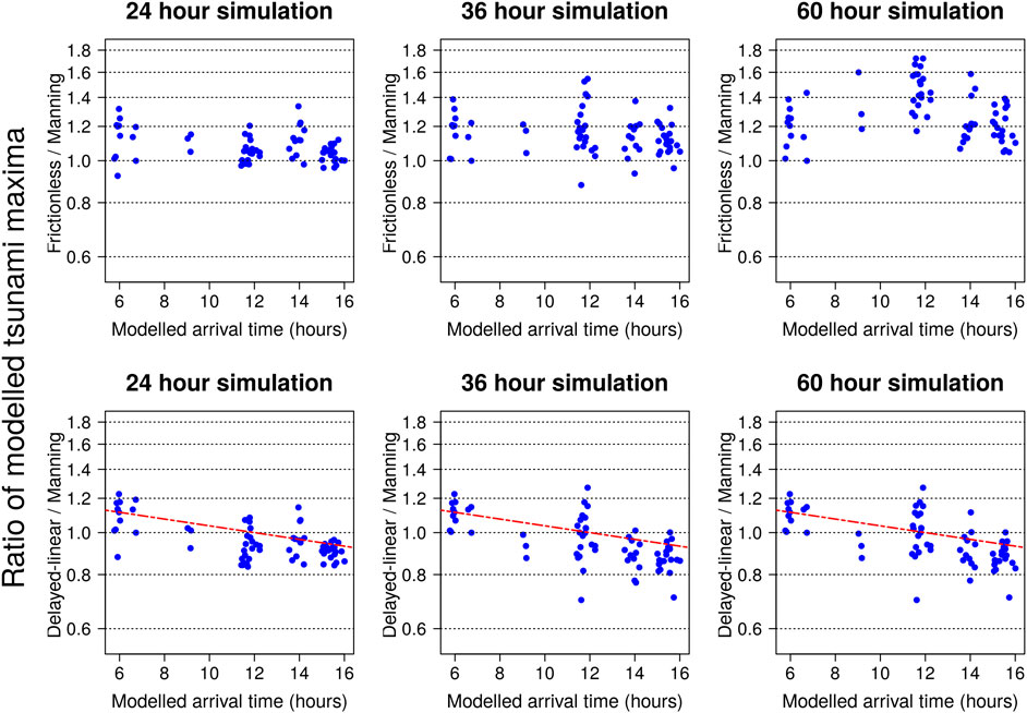
FIGURE 13. Ratios of modeled tsunami maxima, at nearshore sites with tide-gauge data, using different offshore friction treatments: Top row frictionless/Manning; Bottom row Delayed-linear-friction/Manning-friction. In the bottom row the dashed line is $y=1/\text{exp}\left(-f\left(t_{12}-t_a\right)/2\right)$ where $t_a$ is the modeled gauge-specific tsunami arrival time and $t_{12}$ is the number of seconds in 12 h; this is a linear approximation of the proportionate reduction in the delayed-linear-friction tsunami maxima if the initial frictionless period was $t_a$ instead of $t_{12}$ (under various assumptions appropriate for our sites, as discussed in the text).

In some instances unit-source based treatments of global tsunami propagation are essential; for example if many tsunami scenarios must be simulated for a small nearshore area, global propagation modeling may be computationally prohibitive. In such circumstances the delayed-linear friction model is worth considering, particularly for long simulation durations where biases in the frictionless model are anticipated. While not motivated from hydrodynamic theory, this model addresses the early-time bias of constant linear-friction, which was found to underestimate observed tsunami maxima 0–8 h post-arrival. A key result of this study is that the model can be implemented, to high-accuracy, via a trivial transformation of frictionless solutions (Eq. 16). Thus the model is very easy to implement with existing unit-source databases based on the frictionless LSWE (e.g., Thio, 2015; Davies and Griffin, 2020).

Herein delayed-linear-friction was applied with a 12 h frictionless period $\left(t_{12}\right)$, and it is natural to ask if this duration is optimal. Figure 13 (bottom row) shows that while delayed-linear-friction generally predicts tsunami maxima similar to the Manning-friction model, there is a negative correlation between the modeled tsunami arrival time and the ratio of the two models (Figure 13). This result is expected if the Manning-friction model is better approximated using the gauge-specific arrival time $t_a$ to define the frictionless period in Eq. 16 rather than $t_{12}$, i.e.:

$[{\eta }^a,u{h}^a,v{h}^a]=\text{exp}\left(-\frac{f}{2}\text{Max}\left(0,t-t_a\right)\right)[{\eta }^0,u{h}^0,v{h}^0](17)$

One may estimate the relative change r in the tsunami maxima that would result from this approach, vs. the use of $t_{12}$ herein, by assuming the modeled maxima responds linearly to the incoming wave. In this case r is equal to the ratio of Eqs 16 and 17:

$\begin{array}{c}r=\frac{\text{exp}\left(-\frac{f}{2}\text{Max}\left(0,t_M-t_a\right)\right)}{\text{exp}\left(-\frac{f}{2}\text{Max}\left(0,t_M-t_{12}\right)\right)}\\ =\text{exp}\left(-\frac{f}{2}\left(t_{12}-t_a\right)\right)\text{ if }{t}_M>t_{12}\text{ and }{t}_M>t_a\end{array}(18)$

where $t_M$ indicates the timing of the offshore waves controlling the tsunami maxima. The inequality constraints in Eq. 18 should hold for almost all of our delayed-linear-friction modeled gauge-records; only 2/68 modeled time-series in Figure 13 have tsunami maxima arriving before 14 h post-earthquake, or less than 3 h post-tsunami-arrival; only one observed gauge maxima occurs before 18 h post-earthquake (Hillarys for Sumatra 2004; Figure 8). The fact that $1/r$ reasonably approximates the tsunami maxima ratio in Figure 13 suggests that, for site-specific studies, the Manning-friction results may be better approximated with delayed-linear-friction using a “local” initial frictionless period defined by $t_a$. This “local” approach was not implemented herein because a wide range of sites were modeled simultaneously, each having their own $t_a$ (Figure 3). However it would be straightforward to apply in site-specific studies, and merits further testing.

Finally we emphasize limitations of this study and directions for further work. All results are based on global-scale propagation models with little numerical dissipation. Clearly these techniques should not be applied to models where numerical dissipation is already comparable to or greater than the required physical dissipation, as this could exaggerate any under-estimation of late arriving waves. Our models neglect various physical processes which can affect tsunami propagation (dispersion, loading, self-gravitation, density stratification), and we make no attempt to resolve coastal inundation outside our areas of interest in Australia although this may affect remote wave reflections; future work should consider the influence of these approximations on modeled waves at the coast. Following previous work (Allen and Greenslade, 2016; Adams and LeVeque, 2017) we used the tsunami-maxima statistic to quantify model biases, and while this is useful, there is much more information available in the full time-series that may be extracted using other statistics and provide new insights into the model performance. The tests herein consider only five historic tsunamis using sources derived from 12 finite-fault inversions, with a total of 28 tide-gauge records. The testing should be extended to consider more historic events and sites, and other types of data (e.g., inundation footprints and depths; tsunami currents). Of particular interest is the global-record of historical tsunami energy-decay timescales (e.g., van Dorn, 1987; Rabinovich et al., 2011, 2013); further insights into dissipation models would likely be obtained by simulating these observations with alternative models. The tests should also be extended to consider tsunami scenarios derived for hazard assessment (Davies, 2019), including characterization of the nearshore performance of random hazard scenarios.

5.Conclusion

When modeling far-field tsunamis in the nearshore it is often convenient to nest high-resolution nonlinear shallow water models (which cover coastal regions of interest) within reduced-physics global-scale models (which efficiently simulate tsunami propagation). In this context we evaluated the performance of several reduced-physics global propagation models which combine the LSWE with alternative treatments of friction. Nearshore tsunamis were simulated with a nested nonlinear model and compared with coastal tide-gauge observations in Australia. Tsunami initial conditions were derived from published source-models. Our results suggest the commonly used frictionless global-scale model is adequate for simulating far-field coastal tsunamis for 0–8 h following arrival. However for sufficiently long simulations the frictionless model overestimates coastal wave heights because it is mathematically energy conservative (which is well approximated with our numerical methods) and thus does not represent global-scale tsunami dissipation. In our simulations this bias was clear from comparison with data 36–60 h post-earthquake; it is difficult to define a precise time at which the bias becomes significant. Better estimates of late-time wave heights can be obtained by appending Manning-friction to the global model, although this renders the model nonlinear. For unit-source based implementations it is preferable work with linear models, and so variants of linear-friction were tested; these are not derived from hydrodynamic theory yet can mimic observed tsunami energy decay rates. Among these, delayed-linear-friction most accurately simulated tsunami maxima at nearshore gauges. Solutions of this model can be conveniently derived by transforming frictionless LSWE solutions with Eq. 16, making it easy to implement via existing unit-source databases that are derived with the frictionless LSWE (e.g., Davies and Griffin, 2020). These results may facilitate improved simulation of late-time tsunami wave heights for hazard and early warning applications in the far-field.

Data Availability Statement

The datasets presented in this study can be found in online repositories. The names of the repository/repositories and accession number(s) can be found below: https://github.com/GeoscienceAustralia/ptha/tree/master/misc/nearshore_testing_2020.

Author Contributions

GD led the study design and implementation and wrote the first draft manuscript, with guidance from FR and SL. FR provided code and data to construct the sources R14 and R16. All authors contributed to the final manuscript.

Acknowledgments

This paper was published with the permission of the CEO, Geoscience Australia, and was undertaken with the assistance of resources and services from the National Computational Infrastructure (NCI), which is supported by the Australian Government. Discussions with Jon Hinwood and reviews by Kaya Wilson, Phil Cummins, Alexander Rabinovich and Efim Pelinovsky improved the work. Tide-gauge data was provided by the NSW Department of Planning, Industry and Environment, Manly Hydraulics Laboratory, the NSW Port Authority, the WA Department of Transport, and the Australian Bureau of Meteorology. The elevation data was based on a range of elevation products available from ELVIS http://elevation.fsdf.org.au/, The Australian Oceans Data Network https://portal.aodn.org.au/, Ausseabed http://www.ausseabed.gov.au/data, and the WA Department of Transport https://catalogue.data.wa.gov.au/dataset/composite-surfaces-multibeam-lidar-laser.

Conflict of Interest

The authors declare that the research was conducted in the absence of any commercial or financial relationships that could be construed as a potential conflict of interest.

References

Adams, L. M., and LeVeque, R. J. (2017). Technical Report. GeoClaw model tsunamis Compared to tide gauge results, final report. University of Washington (Accessed November 3, 2017).

Google Scholar

Allen, S. C. R., and Greenslade, D. J. M. (2016). A pilot tsunami inundation forecast system for Australia. Pure Appl. Geophys. 173, 3955–3971. doi:10.1007/s00024-016-1392-y

CrossRef Full Text | Google Scholar

Allgeyer, S., and Cummins, P. (2014). Numerical tsunami simulation including elastic loading and seawater density stratification. Geophys. Res. Lett. 41, 2368–2375. doi:10.1002/2014GL059348

CrossRef Full Text | Google Scholar

An, C., and Liu, P. L.-F. (2016). Analytical solutions for estimating tsunami propagation speeds. Coastal Engg. 117, 44–56. doi:10.1016/j.coastaleng.2016.07.006

CrossRef Full Text | Google Scholar

Anderson, S. (2015). Tsunami: the ultimate guide. Aust. J. Emerg. Manag. 30, 24–41.

Google Scholar

Arakawa, A., and Hsu, Y. G. (1990). Energy conserving and potential-enstrophy dissipating schemes for the shallow water equations. Mon. Weather Rev. 118, 1960–1969. doi:10.1175/1520-0493(1990)118<1960:ECAPED>2.0.CO;2

CrossRef Full Text | Google Scholar

Audusse, E., Bouchut, F., Bristeau, M.-O., Klein, R., and Perthame, B. (2004). A fast and stable well-balanced scheme with hydrostatic reconstruction for shallow water flows. SIAM J. Sci. Comput. 25, 2050–2065. doi:10.1137/s1064827503431090

CrossRef Full Text | Google Scholar

Baba, T., Allgeyer, S., Hossen, J., Cummins, P. R., Tsushima, H., Imai, K., et al. (2017). Accurate numerical simulation of the far-field tsunami caused by the 2011 Tohoku earthquake, including the effects of Boussinesq dispersion, seawater density stratification, elastic loading, and gravitational potential change. Ocean Model. 111, 46–54. doi:10.1016/j.ocemod.2017.01.002

CrossRef Full Text | Google Scholar

Baba, T., Takahashi, N., Kaneda, Y., Ando, K., Matsuoka, D., and Kato, T. (2015). Parallel implementation of dispersive tsunami wave modeling with a nesting algorithm for the 2011 tohoku tsunami. Pure Appl. Geophys. 172, 3455–3472. doi:10.1007/s00024-015-1049-2

CrossRef Full Text | Google Scholar

Baba, T., Takahashi, N., Kaneda, Y., Inazawa, Y., and Kikkojin, M. (2014). “Tsunami inundation modeling of the 2011 tohoku earthquake using three-dimensional building data for Sendai, Miyagi prefecture, Japan,” in Tsunami events and lessons learned. Editors Kontar, Y. A., Takahashi, T., and Santiago-Fandino, V. (Amsterdam: Springer).

Google Scholar

Beccari, B. (2009). Technical Report. Measurements and impacts of the Chilean tsunami of may 1960 in new south wales, Australia. NSW State Emergency Service.

Google Scholar

Behrens, J., and Dias, F. (2015). New computational methods in tsunami science. Philos. Trans. R. Soc. London A 373, 20140382. doi:10.1098/rsta.2014.0382

CrossRef Full Text | Google Scholar

Borrero, J. C., Goring, D. G., Greer, S. D., and Power, W. L. (2015a). Far-field tsunami hazard in New Zealand ports. Pure Appl. Geophys. 172, 731–756. doi:10.1007/s00024-014-0987-4

CrossRef Full Text | Google Scholar

Borrero, J. C., Lynett, P. J., and Kalligeris, N. (2015b). Tsunami currents in ports. Phil. Trans. Math. Phys. Eng. Sci. 373, 20140372. doi:10.1098/rsta.2014.0372

CrossRef Full Text | Google Scholar

Buijsman, M., Arbic, B., Green, J., Helber, R., Richman, J., Shriver, J., et al. (2015). Optimizing internal wave drag in a forward barotropic model with semidiurnal tides. Ocean Model. 85, 42–55. doi:10.1016/j.ocemod.2014.11.003

CrossRef Full Text | Google Scholar

Burbidge, D., Cummins, P., Mleczko, R., and Thio, H. (2008). A probabilistic tsunami hazard assessment for western Australia. Pure Appl. Geophys. 165, 2059–2088. doi:10.1007/s00024-008-0421-x

CrossRef Full Text | Google Scholar

Choi, B. H., Pelinovsky, E., Kim, K. O., and Lee, J. S. (2003). Simulation of the trans-oceanic tsunami propagation due to the 1883 krakatau volcanic eruption. Nat. Hazards Earth Syst. Sci. 3, 321–332. doi:10.5194/nhess-3-321-2003

CrossRef Full Text | Google Scholar

Davies, G., Griffin, J., Løvholt, F., Glimsdal, S., Harbitz, C., Thio, H. K., et al. (2017). A global probabilistic tsunami hazard assessment from earthquake sources. Geol. Soc. London Spec. Publ. 456, 219–244. doi:10.1144/sp456.5

CrossRef Full Text | Google Scholar

Davies, G., and Griffin, J. (2018). Technical Report, Geoscience Australia Record 2018/41. The 2018 Australian probabilistic tsunami hazard assessment: hazards from earthquake generated tsunamis. doi:10.11636/Record.2018.041

CrossRef Full Text | Google Scholar

Davies, G., and Griffin, J. (2020). Sensitivity of probabilistic tsunami hazard assessment to far-field earthquake slip complexity and rigidity depth-dependence: case study of Australia. Pure Appl. Geophys. 177, 1521–1548. doi:10.1007/s00024-019-02299-w

CrossRef Full Text | Google Scholar

Davies, G., and Roberts, S. (2015). Open source flood simulation with a 2D discontinuous-elevation hydrodynamic model. Proc. of MODSIM 2015, GoldCoast. doi:10.36334/modsim.2015.l5.davies.

CrossRef Full Text | Google Scholar

Davies, G. (2019). Tsunami variability from uncalibrated stochastic earthquake models: tests against deep ocean observations 2006-2016. Geophys. J. Int. 218, 1939–1960. doi:10.1093/gji/ggz260

CrossRef Full Text | Google Scholar

Egbert, G. D., and Erofeeva, S. Y. (2002). Efficient inverse modeling of barotropic ocean tides. J. Atmos. Ocean. Technol. 19, 183–204. doi:10.1175/1520-0426(2002)019〈0183:EIMOBO〉2.0.CO;2

CrossRef Full Text | Google Scholar

Egbert, G. D., and Ray, R. D. (2000). Significant dissipation of tidal energy in the deep ocean inferred from satellite altimeter data. Nature 405, 775–778. doi:10.1038/35015531

CrossRef Full Text | Google Scholar

Fine, I. V., Kulikov, E. A., and Cherniawsky, J. Y. (2013). Japans 2011 tsunami: characteristics of wave propagation from observations and numerical modelling. Pure Appl. Geophys. 170, 1295–1307. doi:10.1007/s00024-012-0555-8

CrossRef Full Text | Google Scholar

Fjordholm, U. S., Mishra, S., and Tadmor, E. (2011). Well-balanced and energy stable schemes for the shallow water equations with discontinuous topography. J. Comput. Phys. 230, 5587–5609. doi:10.1016/j.jcp.2011.03.042

CrossRef Full Text | Google Scholar

Fritz, H. M., and Borrero, J. C. (2006). Somalia field survey after the december 2004 Indian ocean tsunami. Earthq. Spectra. 22, 219–233. doi:10.1193/1.2201972

CrossRef Full Text | Google Scholar

Fujii, Y., and Satake, K. (2007). Tsunami source of the 2004 sumatra-andaman earthquake inferred from tide gauge and satellite data. Bull. Seismol. Soc. Am. 97, S192. doi:10.1785/0120050613

CrossRef Full Text | Google Scholar

Fujii, Y., and Satake, K. (2013). Slip distribution and seismic moment of the 2010 and 1960 Chilean earthquakes inferred from tsunami waveforms and coastal geodetic data. Pure Appl. Geophys. 170, 1493–1509. doi:10.1007/s00024-012-0524-2

CrossRef Full Text | Google Scholar

Geist, E. (2009). Phenomenology of tsunamis: statistical properties from generation to runup. Adv. Geophys. 51, 107–169. doi:10.1016/S0065-2687(09)05108-5

CrossRef Full Text | Google Scholar

Gica, E., Spillane, M. C., Titov, V. V., Chamberlin, C. D., and Newman, J. C. (2008). Technical Report No. 139. Development of the forecast propagation database for NOAA’s short-term inundation forecast for tsunamis (SIFT). NOAA Technical Memorandum OAR PMEL, Seattle, WA.

Google Scholar

Glimsdal, S., Pedersen, G., Harbitz, C., and Løvholt, F. (2013). Dispersion of tsunamis: does it really matter? Nat. Hazards Earth Syst. Sci. 13, 1507–1526. doi:10.5194/nhess-13-1507-2013

CrossRef Full Text | Google Scholar

Goto, C., and Ogawa, Y. (1997). Technical Report No. 35. Numerical method of tsunami simulation with the leap-frog scheme. IUGG/IOC Time Project.

Google Scholar

Greenslade, D. J. M., Allen, S. C. R., and Simanjuntak, M. A. (2011). An evaluation of tsunami forecasts from the T2 scenario database. Pure Appl. Geophys. 168, 1137–1151. doi:10.1007/s00024-010-0229-3

CrossRef Full Text | Google Scholar

Grezio, A., Babeyko, A., Baptista, M. A., Behrens, J., Costa, A., Davies, G., et al. (2017). Probabilistic tsunami hazard analysis: multiple sources and global applications. Rev. Geophys. 55, 1158–1198. doi:10.1002/2017RG000579. 2017RG000579

CrossRef Full Text | Google Scholar

Heidarzadeh, M., Satake, K., Takagawa, T., Rabinovich, A., and Kusumoto, S. (2018). A comparative study of far-field tsunami amplitudes and ocean-wide propagation properties: insight from major trans-Pacific tsunamis of 2010-2015. Geophys. J. Int. 215, 22–36. doi:10.1093/gji/ggy265

CrossRef Full Text | Google Scholar

Hinwood, J. B., and Mclean, E. J. (2013). Effects of the march 2011 Japanese tsunami in bays and estuaries of SE Australia. Pure Appl. Geophys. 170, 1207–1227. doi:10.1007/s00024-012-0561-x

CrossRef Full Text | Google Scholar

Ho, T.-C., Satake, K., Watada, S., and Fujii, Y. (2019). Source estimate for the 1960 Chile earthquake from joint inversion of geodetic and transoceanic tsunami data. J. Geophys. Res. Solid Earth. 124, 2812–2828. doi:10.1029/2018JB016996

CrossRef Full Text | Google Scholar

Kânoğlu, U., Titov, V., Bernard, E., and Synolakis, C. (2015). Tsunamis: bridging science, engineering and society. Philos. Trans. R. Soc. London. 373, 20140369. doi:10.1098/rsta.2014.0369

CrossRef Full Text | Google Scholar

Kajiura, K. (1963). The leading wave of a tsunami. Bull. Earthq. Res. Inst. 41, 535–571.

Google Scholar

Kleermaeker, S. D., Apecechea, M. I., Verlaan, M., Mortlock, T., and Rego, J. L. (2019). “Global-to-local scale storm surge modelling: operational forecasting and model sensitivities,” in Australasian coasts & ports 2019 conference, Hobart, September 10–13, 2019.

Google Scholar

Kowalik, Z., Horrillo, J., Knight, W., and Logan, T. (2008). Kuril Islands tsunami of november 2006: 1. Impact at crescent city by distant scattering. J. Geophys. Res. 113, C01020. doi:10.1029/2007JC004402

CrossRef Full Text | Google Scholar

Kulikov, E. A., Fine, I. V., and Yakovenko, O. I. (2014). Numerical modeling of the long surface waves scattering for the 2011 Japan tsunami: case study. Izvestiya Atmos. Ocean. Phys. 50, 498–507. doi:10.1134/S0001433814050053

CrossRef Full Text | Google Scholar

Kulikov, E. (2006). Dispersion of the Sumatra Tsunami waves in the Indian Ocean detected by satellite altimetry. Russ. J. Earth Sci. 8, 1–5. doi:10.2205/2006es000214

CrossRef Full Text | Google Scholar

Li, L., Switzer, A. D., Chan, C.-H., Wang, Y., Weiss, R., and Qiu, Q. (2016). How heterogeneous coseismic slip affects regional probabilistic tsunami hazard assessment: a case study in the South China Sea. J. Geophys. Res. Solid Earth. 121, 6250–6272. doi:10.1002/2016JB013111. 2016JB013111

CrossRef Full Text | Google Scholar

Liu, P. L. F., Cho, Y.-S., Briggs, M. J., Kanoglu, U., and Synolakis, C. E. (1995). Runup of solitary waves on a circular island. J. Fluid Mech. 302, 259–285. doi:10.1017/S0022112095004095

CrossRef Full Text | Google Scholar

Liu, Y., Shi, Y., Yuen, D. A., Sevre, E. O. D., Yuan, X., and Xing, H. L. (2008). Comparison of linear and nonlinear shallow wave water equations applied to tsunami waves over the China sea. Acta Geotechnica. 4, 129–137. doi:10.1007/s11440-008-0073-0

CrossRef Full Text | Google Scholar

Llewellyn Smith, S. G., and Young, W. R. (2002). Conversion of the barotropic tide. J. Phys. Oceanogr. 32, 1554–1566. doi:10.1175/1520-0485(2002)032〈1554:COTBT〉2.0.CO;2

CrossRef Full Text | Google Scholar

Lorenz, E. N. (1955). Available potential energy and the maintenance of the general circulation. Tellus 7, 157–167. doi:10.1111/j.2153-3490.1955.tb01148.x

CrossRef Full Text | Google Scholar

Lorito, S., Piatanesi, A., Cannelli, V., Romano, F., and Melini, D. (2010). Kinematics and source zone properties of the 2004 Sumatra-Andaman earthquake and tsunami: nonlinear joint inversion of tide gauge, satellite altimetry, and GPS data. J. Geophys. Res. 115, B02304. doi:10.1029/2008jb005974

CrossRef Full Text | Google Scholar

Lorito, S., Romano, F., Atzori, S., Tong, X., Avallone, A., McCloskey, J., et al. (2011). Limited overlap between the seismic gap and coseismic slip of the great 2010 Chile earthquake. Nat. Geosci. 4, 173–177. doi:10.1038/ngeo1073

CrossRef Full Text | Google Scholar

Lorito, S., Selva, J., Basili, R., Romano, F., Tiberti, M., and Piatanesi, A. (2015). Probabilistic hazard for seismically induced tsunamis: accuracy and feasibility of inundation maps. Geophys. J. Int. 200, 574–588. doi:10.1093/gji/ggu408

CrossRef Full Text | Google Scholar

Macías, J., Castro, M. J., Ortega, S., and González-Vida, J. M. (2020). Performance assessment of Tsunami-HySEA model for NTHMP tsunami currents benchmarking. Field cases. Ocean Model. 152, 101645. doi:10.1016/j.ocemod.2020.101645

CrossRef Full Text | Google Scholar

Meade, B. J. (2007). Algorithms for the calculation of exact displacements, strains, and stresses for triangular dislocation elements in a uniform elastic half space. Comput. Geosci. 33, 1064–1075. doi:10.1016/j.cageo.2006.12.003

CrossRef Full Text | Google Scholar

Miller, G. R., Munk, W. H., and Snodgrass, F. E. (1962). Long-period waves over California’s continental borderland part ii. tsunamis. J. Mar. Res. 20, 31–41.

Google Scholar

Miranda, J. M., Baptista, M. A., and Omira, R. (2014). On the use of Green’s summation for tsunami waveform estimation: a case study. Geophys. J. Int. 199, 459–464. doi:10.1093/gji/ggu266

CrossRef Full Text | Google Scholar

Mofjeld, H. O., González, F. I., Bernard, E. N., and Newman, J. C. (2000). Forecasting the heights of later waves in pacific-wide tsunamis. Nat. Hazards. 22, 71–89. doi:10.1023/A:1008198901542

CrossRef Full Text | Google Scholar

Molinari, I., Tonini, R., Lorito, S., Piatanesi, A., Romano, F., Melini, D., et al. (2016). Fast evaluation of tsunami scenarios: uncertainty assessment for a Mediterranean Sea database. Nat. Hazards Earth Syst. Sci. 16, 2593–2602. doi:10.5194/nhess-16-2593-2016

CrossRef Full Text | Google Scholar

Munk, W. (1963). “Some comments regarding diffusion and absorption of tsunamis,” in Proceedings Tsunami Meetings, Tenth Pacific Science Congress, Honolulu (IUGG Monograph), Vol. 24, 53–72.

Google Scholar

Munk, W. (1997). Once again: once again―tidal friction. Prog. Oceanogr. 40, 7–35. doi:10.1016/S0079-6611(97)00021-9

CrossRef Full Text | Google Scholar

NCI (2020). [Dataset] National computational infrastructure hpc systems. Available at:https://nci.org.au/our-systems/hpc-systems.

Google Scholar

NTHMP(2012). Technical Report. Proceedings and results of the 2011 NTHMP model benchmarking workshop. National Tsunami Hazard Mitigation Program, NOAA Special Report.

Google Scholar

Nyland, D., and Huang, P. (2013). Forecasting wave amplitudes after the arrival of a tsunami. Pure Appl. Geophys. 171, 3501–3513. doi:10.1007/s00024-013-0703-9

CrossRef Full Text | Google Scholar

Oh, I., and Rabinovich, A. (1994). Manifestation of hokkaido southwest (okushiri) tsunami 12 July, 1993, at the coast of korea. Sci. Tsunami Hazards. 12, 93–116.

Google Scholar

Okada, Y. (1985). Surface deformation due to shear and tensile faults in a half-space. Bull. Seismol. Soc. Am. 75, 1135–1154.

Google Scholar

Okal, E. A. (2011). Tsunamigenic earthquakes: past and present milestones. Pure Appl. Geophys. 168, 969–995. doi:10.1007/s00024-010-0215-9

CrossRef Full Text | Google Scholar

Pattiaratchi, C., and Wijeratne, E. M. S. (2009). Tide gauge observations of 2004-2007 Indian Ocean tsunamis from Sri Lanka and Western Australia. Pure Appl. Geophys. 166, 233–258. doi:10.1007/s00024-008-0434-5

CrossRef Full Text | Google Scholar

Percival, D. M., Percival, D. B., Denbo, D. W., Gica, E., Huang, P. Y., Mofjeld, H. O., et al. (2014). Automated tsunami source modeling using the sweeping window positive elastic net. J. Am. Stat. Assoc. 109, 491–499. doi:10.1080/01621459.2013.879062

CrossRef Full Text | Google Scholar

Piatanesi, A., and Lorito, S. (2007). Rupture process of the 2004 sumatra–andaman earthquake from tsunami waveform inversion. Bull. Seismol. Soc. Am. 97, S223–S231. doi:10.1785/0120050627

CrossRef Full Text | Google Scholar

Popinet, S. (2011). Quadtree-adaptive tsunami modelling. Ocean Dynam. 61, 1261–1285. doi:10.1007/s10236-011-0438-z

CrossRef Full Text | Google Scholar

Rabinovich, A. B., Candella, R. N., and Thomson, R. E. (2011). Energy decay of the 2004 Sumatra tsunami in the world ocean. Pure Appl. Geophys. 168, 1919–1950. doi:10.1007/s00024-011-0279-1

CrossRef Full Text | Google Scholar

Rabinovich, A. B., Candella, R. N., and Thomson, R. E. (2013). The open ocean energy decay of three recent trans-pacific tsunamis. Geophys. Res. Lett. 40, 3157–3162. doi:10.1002/grl.50625

CrossRef Full Text | Google Scholar

Romano, F., Piatanesi, A., Lorito, S., Tolomei, C., Atzori, S., and Murphy, S. (2016). Optimal time alignment of tide-gauge tsunami waveforms in nonlinear inversions: application to the 2015 Illapel (Chile) earthquake. Geophys. Res. Lett. 43, 11226–11235. doi:10.1002/2016GL071310. 2016GL071310

CrossRef Full Text | Google Scholar

Romano, F., Trasatti, E., Lorito, S., Piromallo, C., Piatanesi, A., Ito, Y., et al. (2014). Structural control on the Tohoku earthquake rupture process investigated by 3D FEM, tsunami and geodetic data. Sci. Rep. 4, 5631. doi:10.1038/srep05631

CrossRef Full Text | Google Scholar

Saito, T., Inazu, D., Miyoshi, T., and Hino, R. (2014). Dispersion and nonlinear effects in the 2011 Tohoku-oki earthquake tsunami. J. Geophys. Res. Oceans. 119, 5160–5180. doi:10.1002/2014jc009971

CrossRef Full Text | Google Scholar

Satake, K., Fujii, Y., Harada, T., and Namegaya, Y. (2013). Time and space distribution of coseismic slip of the 2011 tohoku earthquake as inferred from tsunami waveform data. Bull. Seismol. Soc. Am. 103, 1473–1492. doi:10.1785/0120120122

CrossRef Full Text | Google Scholar

Satake, K., Okada, M., and Abe, K. (1988). Tide gauge response to tsunamis: measurements at 40 tide gauge stations in Japan. J. Mar. Res. 46, 557–571. doi:10.1357/002224088785113504

CrossRef Full Text | Google Scholar

Setiyono, U., Gusman, A. R., Satake, K., and Fujii, Y. (2017). Pre-computed tsunami inundation database and forecast simulation in Pelabuhan Ratu, Indonesia. Pure Appl. Geophys. 174, 3219–3235. doi:10.1007/s00024-017-1633-8

CrossRef Full Text | Google Scholar

Shuto, N. (1991). Numerical simulation of tsunamis—its present and near future. Nat. Hazards. 4, 171–191. doi:10.1007/BF00162786

CrossRef Full Text | Google Scholar

Tang, L., Titov, V. V., Bernard, E. N., Wei, Y., Chamberlin, C. D., Newman, J. C., et al. (2012). Direct energy estimation of the 2011 Japan tsunami using deep-ocean pressure measurements. J. Geophys. Res.: Oceans. 117, C08008. doi:10.1029/2011JC007635

CrossRef Full Text | Google Scholar

Tang, L., Titov, V. V., and Chamberlin, C. D. (2009). Development, testing, and applications of site-specific tsunami inundation models for real-time forecasting. J. Geophys. Res. 114, C12025. doi:10.1029/2009JC005476

CrossRef Full Text | Google Scholar

Tanioka, Y., and Satake, K. (1996). Tsunami generation by horizontal displacement of ocean bottom. Geophys. Res. Lett. 23, 861–864. doi:10.1029/96GL00736

CrossRef Full Text | Google Scholar

Thio, H. (2015). “Tsunami hazards of the pacific rim,” in Proceedings of the 10th pacific conference on earthquake engineering, Sydney, November 6–8, 2015

Google Scholar

Titov, V., Song, Y. T., Tang, L., Bernard, E. N., Bar-Sever, Y., and Wei, Y. (2016). Consistent estimates of tsunami energy show promise for improved early warning. Pure Appl. Geophys. 173, 3863–3880. doi:10.1007/s00024-016-1312-1

CrossRef Full Text | Google Scholar

Tolkova, E. (2014). Land-water boundary treatment for a tsunami model with dimensional splitting. Pure Appl. Geophys. 171, 2289–2314. doi:10.1007/s00024-014-0825-8

CrossRef Full Text | Google Scholar

Tolkova, E. (2015). Tsunami penetration in tidal rivers, with observations of the Chile 2015 tsunami in rivers in Japan. Pure Appl. Geophys. 173, 389–409. doi:10.1007/s00024-015-1229-0

CrossRef Full Text | Google Scholar

van Dorn, W. G. (1984). Some tsunami characteristics deducible from tide records. J. Phys. Oceanogr. 14, 353–363. doi:10.1175/1520-0485(1984)014〈0353:STCDFT〉2.0.CO;2

CrossRef Full Text | Google Scholar

van Dorn, W. G. (1987). Tide gauge response to tsunamis. part 2: other oceans and smaller seas. J. Phys. Oceanogr. 17, 1507–1516. doi:10.1175/1520-0485(1987)017<1507:TGRTTP>2.0.CO;2

CrossRef Full Text | Google Scholar

Volpe, M., Lorito, S., Selva, J., Tonini, R., Romano, F., and Brizuela, B. (2019). From regional to local SPTHA: efficient computation of probabilistic tsunami inundation maps addressing near-field sources. Nat. Hazards Earth Syst. Sci. 19, 455–469. doi:10.5194/nhess-19-455-2019

CrossRef Full Text | Google Scholar

Watada, S., Kusumoto, S., and Satake, K. (2014). Traveltime delay and initial phase reversal of distant tsunamis coupled with the self-gravitating elastic earth. J. Geophys. Res. Solid Earth. 119, 4287–4310. doi:10.1002/2013jb010841

CrossRef Full Text | Google Scholar

Weatherall, P., Marks, K. M., Jakobsson, M., Schmitt, T., Tani, S., Arndt, J. E., et al. (2015). A new digital bathymetric model of the world’s oceans. Earth Space Sci. 2, 331–345. doi:10.1002/2015EA000107

CrossRef Full Text | Google Scholar

Whiteway, T. (2009). Technical Report, Geoscience Australia Record 2009/21. Australian bathymetry and topography grid, June 2009.

Google Scholar

Williamson, A., Newman, A., and Cummins, P. (2017). Reconstruction of coseismic slip from the 2015 Illapel earthquake using combined geodetic and tsunami waveform data. J. Geophys. Res. 122, 2119–2130. doi:10.1002/2016JB013883

CrossRef Full Text | Google Scholar

Wilson, K. M., Allen, S. C. R., and Power, H. E. (2018). The tsunami threat to Sydney Harbour, Australia: modelling potential and historic events. Sci. Rep. 8, 15045. doi:10.1038/s41598-018-33156-w

CrossRef Full Text | Google Scholar

Wilson, K. M., and Power, H. E. (2018). Seamless bathymetry and topography datasets for new south wales, Australia. Scientific Data. 5, 180115. doi:10.1038/sdata.2018.115

CrossRef Full Text | Google Scholar

Yamazaki, Y., Cheung, K. F., and Lay, T. (2018). A self-consistent fault slip model for the 2011 tohoku earthquake and tsunami. J. Geophys. Res. Solid Earth. 123, 1435–1458. doi:10.1002/2017JB014749

CrossRef Full Text | Google Scholar

Yue, H., Lay, T., Li, L., Yamazaki, Y., Cheung, K. F., Rivera, L., et al. (2015). Validation of linearity assumptions for using tsunami waveforms in joint inversion of kinematic rupture models: application to the 2010 MentawaiMw7.8 tsunami earthquake. J. Geophys. Res. Solid Earth. 120, 1728–1747. doi:10.1002/2014jb011721

CrossRef Full Text | Google Scholar

Zhang, X., and Niu, X. (2020). Probabilistic tsunami hazard assessment and its application to southeast coast of Hainan Island from Manila Trench. Coastal Engg. 155, 103596. doi:10.1016/j.coastaleng.2019.103596

CrossRef Full Text | Google Scholar