Improving Detectability of Seafloor Deformation From Bottom Pressure Observations Using Numerical Ocean Models

Introduction

A quartz-crystal resonator was developed to measure absolute pressure changes with nano resolutions (Irish and Snodgrass, 1972; Wearn and Larson, 1982; Yilmaz et al., 2004). The technique has been applied to measure the absolute pressure changes at deep-sea (∼103 m) bottom (Munk and Zetler, 1967; Nowroozi et al., 1969; Filloux, 1971). The ocean bottom pressure (OBP) observations have been increasingly carried out for various applications in geophysics (Inazu and Hino, 2011; Webb and Nooner, 2016; Paros, 2017): tsunamis (Filloux et al., 1983; Rabinovich and Eblé, 2015; Kubota et al., 2019), seismic/elastic vibrations of sea bottom and of ocean water (Nosov and Kolesov, 2007; Kubota et al., 2017; Nosov et al., 2018), tides (Munk et al., 1970; Eble and Gonzalez, 1991; Mofjeld et al., 1995), offshore storm surges (Beardsley et al., 1977; Mofjeld et al., 1996; Bailey et al., 2014), ocean currents (Chereskin et al., 2009; Park et al., 2010; Nagano et al., 2018), gravity variations (Park et al., 2008; Siegismund et al., 2011; Peralta-Ferriz et al., 2016), and seafloor vertical deformation due to submarine volcanos (Fox, 1999; Chadwick et al., 2012; Sasagawa et al., 2016) and earthquakes (Baba et al., 2006; Ito et al., 2011; Kubota et al., 2018; Itoh et al., 2019).

When elastic oscillations are not considered, the OBP is regarded as static pressure, and its recording (P_B(t)) at a location is represented as follows (Inazu et al., 2012):

$P_B\left(t\right)=P_{\text{ref}}+\Delta P_B\left(t\right),(1)$

$\Delta P_B\left(t\right)=\Delta P_C\left(t\right)+\Delta P_T\left(t\right)+\Delta P_O\left(t\right)+\Delta P_A\left(t\right)+\Delta P_D\left(t\right)+\epsilon \left(t\right).(2)$

ΔP_B(t) is pressure deviations around a reference pressure level according to the sea depth (P_ref), and is decomposed into geophysical and non-geophysical components. ΔP_C(t) indicates the seafloor vertical crustal deformation. ΔP_T(t) indicates the tides. ΔP_O(t) indicates the oceanic variations. ΔP_A(t) indicates the atmospheric pressure loading on sea surface. ΔP_D(t) indicates the non-geophysical, instrumental drifts (Watts and Kontonyanis, 1990; Polster et al., 2009; Kajikawa and Kobata, 2019). ε(t) indicates residuals. The increase of 1 hPa in OBP is equivalent to the elevation of 1 cm in sea level or the subsidence of 1 cm in seafloor below OBP observation point.

When one investigates a particular phenomenon using OBP records, other components need to be estimated and removed. When dominant frequency of the target phenomenon is far from that of other noisy components, the target phenomenon is easily isolated using a Fourier analysis. However, time scales of slow seafloor deformation are comparable to those of oceanic variations. In particular, slow earthquakes with fault slips involve time scales of days to months and/or longer scales (Hirose and Obara, 2005). Vertical seafloor displacements associated with such slow slips are expected to be less than a few centimeters (Ohta et al., 2012) while oceanic variations are up to tens of centimeters in these time scales (Niiler et al., 1993; Donohue et al., 2010). Isolating slow seafloor deformation signals from OBP records is difficult.

Possible relationships between huge earthquakes and aseismic, slow earthquakes/slips at plate boundaries have been investigated and suggested (Ruiz et al., 2014; Tanaka et al., 2019; Baba et al., 2020). Seismological and geodetic efforts have been made to conduct campaign and continuous observations including OBP at the deep-sea bottom near the plate boundaries (Hirata et al., 2002; Hino et al., 2009; Kaneda et al., 2015; Wallace et al., 2016). It is necessary to develop suitable methods of separating slow seafloor deformation and oceanic variation in OBP observations.

We may suppose that spatial scales of earthquake slips (<10² km) (Ohta et al., 2012; Sato et al., 2017) are mostly shorter than those of oceanic variations (>10² km) in time scales of days to months (Niiler et al., 1993; Donohue et al., 2010). When spatially dense OBP observations are carried out, based on this assumption, one can take approaches to cancel (unknown) oceanic variations by simply differentiating nearby OBP stations from a reference OBP station (Ito et al., 2013; Ariyoshi et al., 2014; Wallace et al., 2016; Sato et al., 2017), or by estimating spatially-common components using statistical and/or machine learning methods (Emery and Thomson, 2001; Hino et al., 2014; He et al., 2020).

On the other hand, removing oceanic and other components from single OBP record is a straightforward approach. Tidal signals have been precisely estimated by observed records or numerical predictions (Tamura et al., 1991; Egbert and Erofeeva, 2002). Lower-frequency, non-tidal oceanic variations can be estimated by numerical ocean models, but their accuracy is not typically sufficient for detection of slow slips of less than a few centimeters in OBP observations (Fredrickson et al., 2019; Gomberg et al., 2019; Muramoto et al., 2019). Nevertheless, this approach of reducing ambient oceanic noises is fundamental, and is suitably applied for both multiple-station and single-station observations.

During this decade, there have been extensive OBP observations installed for seismic/geodetic monitoring of shallow plate subduction zones around the Pacific Ocean (Figure 1). Seafloor deformation due to slow slip has been found at a few specific regions and events (Ohta et al., 2012; Ito et al., 2013; Davis et al., 2015; Suzuki et al., 2016; Wallace et al., 2016). However, there was no report on general evaluations of detectability of slow seafloor deformation using OBP observations. Regional dependence of the detectability is not known. Accuracy of used numerical ocean models is not known in terms of OBP variations. In the present study, we investigate the current status of improving detectability of slow seafloor deformation using OBP observations. We utilize OBP data at several subduction zones around the Pacific Ocean, and available numerical ocean prediction models. The detectability is evaluated by root-mean-square (RMS) amplitude (i.e., standard deviation) of residual OBP time series at respective stations.

FIGURE 1

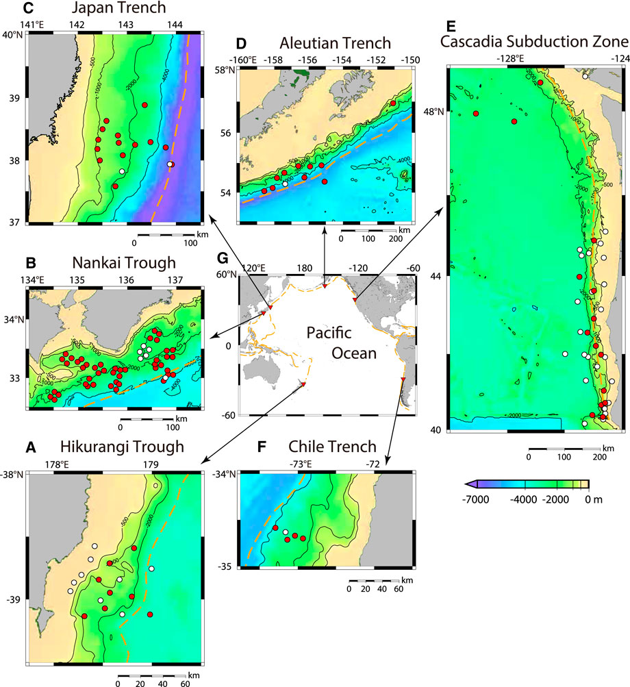
FIGURE 1. Ocean bottom pressure observations at six subduction zones around the Pacific Ocean. The six subduction zones are (A) the Hikurangi Trough, (B) the Nankai Trough, (C) the Japan Trench, (D) the Aleutian Trench, (E) the Cascadia Subduction Zone, and (F) the Chile Trench. (G) shows the map of the Pacific Ocean with specific trench/trough axes (orange dashed lines) derived from Bird (2003). Red and white circles denote used and unused stations, respectively. See Table 1 for detail. Isobaths of 500, 1,000, 2,000, and 4,000 m are shown.

Ocean Bottom Pressure Observations

We use OBP data listed in Table 1. Most of the OBP data are available at the Ocean Bottom Seismograph Instrument Pool (OBSIP) (http://www.obsip.org/). Data obtained at the Japan Trench were provided by Tohoku University (Hino et al., 2009; Hino et al., 2014). These were composed of campaign observations using pop-up-type autonomous gauges. DONET1/2 in Japan (Kaneda et al., 2015) and NEPTUNE-Canada (Barnes et al., 2015) are operated as seafloor cabled systems for long-term (>5 years) continuous observations. These observations are located at six subduction zones around the Pacific Ocean (Figure 1; Table 1). The S-net cabled observatory was installed along the Japan Trench and the Kuril Trench, and the observed data have recently become available (Aoi et al., 2020). However, the S-net OBP data are currently undergoing quality control (Kubota et al., 2020), and are not used in the present study.

TABLE 1

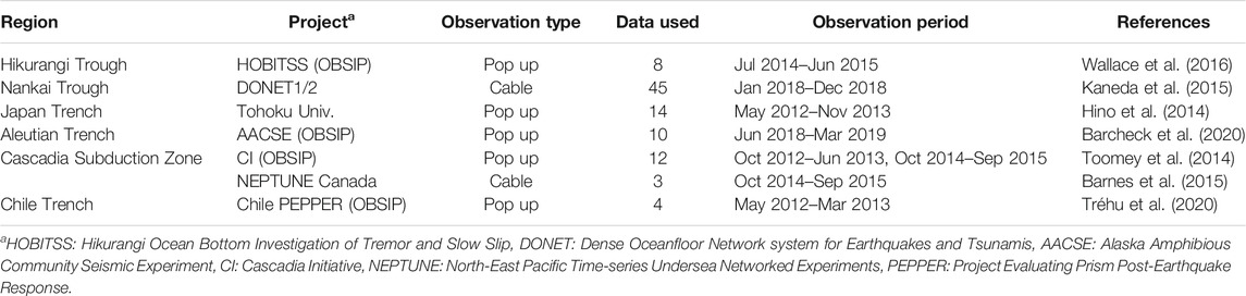
TABLE 1. OBP observations and data.

Far offshore OBP observations are more sensitive to offshore fault motions than onshore Global Navigation Satellite System observations. We investigate the OBP data obtained at sea depths greater than 500 m (Figure 1). In addition, the utilized OBP data consist of approximately year-long continuous records, and we avoid using data with complicated drift or spike noise. In-situ OBP observations include various components as shown by Eq. 2. In the present study, oceanic variations at a period of 3–90 days are extracted using a band-pass filter to remove short-tide components and long-term instrumental drifts. The extracted oceanic variations are compared with numerical ocean models.

Numerical Ocean Models

Numerical ocean models with data assimilation have been developed to realistically predict and estimate oceanic states. Some of them have been available to end users. We use a single-layer ocean model and four multi-layer ocean models (Table 2). The single-layer global ocean model (SOM) was developed by one of the authors (Inazu et al., 2012; Inazu and Saito, 2016). Multi-layer models are referred to as the ocean general circulation models (OGCMs). We use three global models (HYCOM, GLORYS, and ECCO2), and one regional model around Japan (JCOPE2M). Horizontal resolutions are 1/12° for SOM, HYCOM, GLORYS, and JCOPE2M, and ∼18 km for ECCO2. In terms of vertical resolution, these OGCMs contain 40–50 layers. Modeled oceans are driven by external forcing. The SOM is driven by wind and/or atmospheric pressure loading on the sea surface given by the JRA-55 reanalysis (Kobayashi et al., 2015). OGCMs are driven by wind forcing and heat/freshwater flux given by respective reanalysis datasets (Table 2).

TABLE 2

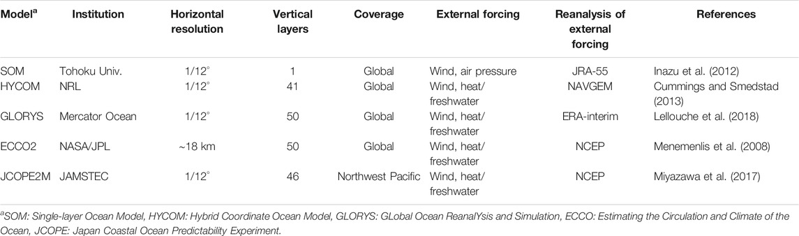
TABLE 2. Numerical ocean models.

Wind stress is the dominant driving force of ocean circulations with disturbances. The wind-driven ocean involves ∼10² cm in sea level variations (i.e., ∼10² hPa in OBP). Only the SOM takes into account the atmospheric pressure loading to drive the ocean. The sea level mostly shows an isostatic response via gravity waves to atmospheric pressure loading (i.e., 1 cm elevation in sea level to 1 hPa depression in atmospheric pressure). This is known as the inverted barometer response (Wunsch and Stammer, 1997). When the inverted barometer response is established, the seafloor hardly feels the atmospheric pressure loading. The inverted barometer response is conventionally assumed especially in deep-sea regions. Heat and freshwater effects on the sea level changes are expected to be relatively small (<1 mm in sea level) in deep-sea regions (Ponte, 2006).

Observed and Modeled Ocean Bottom Pressure

The OBP is shown as an integrated water pressure from sea bottom to sea surface, including atmospheric pressure loading above sea surface. The calculations of OBP are described below for SOM and OGCMs.

According to Inazu et al. (2012), SOM provides sea surface height (η) at each horizontal grid. OBP at a location (P_SOM) is simply given by the pressure due to sea surface height anomaly (η) plus atmospheric pressure loading on sea surface (P_atm):

$P_{\text{SOM}}\left(t\right)={\rho }_{0}g\left(\eta \left(t\right)+H\right)+P_{\text{atm}}\left(t\right),(3)$

where ρ₀, g, and H are constants of seawater density (1,035 kg/m³), gravitational acceleration (9.81 m/s²), and sea depth given at each location, respectively. In the SOM, the wind and the air pressure at sea surface respectively drive the sea surface height and OBP. Figure 2 shows a scheme of sea surface height and OBP driven by wind and air pressure. The sea surface height driven by wind alone (η_w), which is directly projected to OBP (SOM_w = ρ₀gη_w). The sea surface height (η_p) driven by air pressure (P_atm) shows mostly an inverted barometer response. However, there are certain amounts of departures from the inverted barometer in OBP (SOM_p = ρ₀gη_p + P_atm). Note that amplitude of SOM_p is smaller than those of ρ₀gη_p and P_atm, as indicated by Figure 2. The summation of OBP driven by respectively wind and air pressure (SOM_w + SOM_p) is almost the same as the OBP simultaneously driven by wind and pressure (SOM_w+p), indicating that non-linear effects are negligible. Figure 3 shows spatial distributions of RMS amplitudes of OBP driven by wind alone (SOM_w), by air pressure alone (SOM_p), and by both simultaneously (SOM_w+p). SOM_w+p is mostly comparable to SOM_w. However, SOM_p is also evident especially at the Southern Ocean and at marginal seas (Inazu et al., 2006; Ponte and Vinogradov, 2007).

FIGURE 2

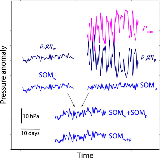
FIGURE 2. Images of pressure variations at sea surface and sea bottom forced by wind and air pressure in SOM. ρ₀gη_w and ρ₀gη_p are sea level variations respectively forced by wind and atmospheric pressure (P_atm) in SOM. SOM_w, SOM_p, and SOM_w+p are resultant ocean bottom pressure variations forced by wind, atmospheric pressure, and both simultaneously.

FIGURE 3

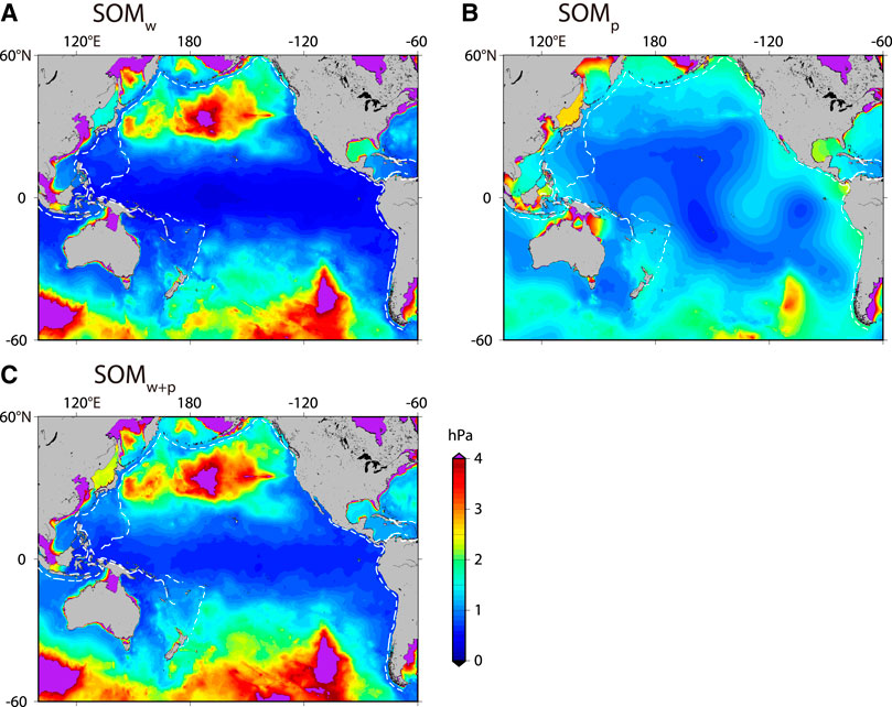
FIGURE 3. Root-mean-square amplitudes of calculated ocean bottom pressure in SOM driven by (A) wind alone, (B) air pressure alone, and (C) both wind and air pressure.

The OGCMs provide sea surface height (η) and temperature/salinity (T/S) at each vertical layer (depth: z), but currently do not include atmospheric pressure loading (i.e., P_atm). We calculate seawater density and pressure using these essential parameters. The EOS-80’s equation of state for seawater (Fofonoff and Millard, 1983) is used to calculate the seawater density (ρ) from T, S, and hydrostatic pressure according to z. Vertical integration from sea bottom to sea surface is carried out to calculate OBP variations with a long-wave, hydrostatic approximation:

$P_{\text{OGCM}}\left(t\right)=g{\displaystyle {\int }_{-H}^{\eta \left(t\right)}\rho \left(t,z,T,S\right)\text{d}z}=g\eta \left(t\right)\rho \left(t,0,T,S\right)+g{\displaystyle {\int }_{-H}^0\rho \left(t,z,T,S\right)\text{d}z}.(4)$

Figure 4 shows an example of the calculation derived from HYCOM. It is evident that sea-surface height pressure (first term of Eq. 4) and sub-surface pressure (second term of Eq. 4) are inversely correlated. This compensation relationship between the sea-surface and the sub-surface pressure is typically predicted in a simplified two-layer ocean model (Gill, 1982; Unoki, 1993). The OBP is shown as an anomaly from the compensation.

FIGURE 4

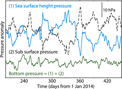
FIGURE 4. Pressure variations derived from sea surface height (light blue), integration below static sea level (black dashed), and both combined (dark green). This is an example of LOBS4 (–39.1201°N, 178.9815°E) at the Hikurangi Trough, which is calculated from HYCOM.

As mentioned above, the calculated OBP from each ocean model is compared with observed OBP data at the period of 3–90 days. Figure 5 shows an example at the Hikurangi Trough. Good agreement is found between the observation and SOM driven by both wind and air pressure (SOM_w+p), as was reported by Muramoto et al. (2019). The agreement is considerably good at periods <10¹ days. A multi-layer model (GLORYS) shows a worse fit to the observation. GLORYS as well as other multi-layer models are driven mainly by the wind forcing, but not by air pressure. Here, we add an OBP component driven by the air pressure alone using SOM (SOM_p) to the GLORYS’s prediction. The agreement between the observed and modeled OBP is notably improved especially at periods <∼10 days. This example indicates that the departure from an inverted barometer (SOM_p) is evident and should be incorporated to more accurately model the OBP at the period of 3–90 days even in the deep sea.

FIGURE 5

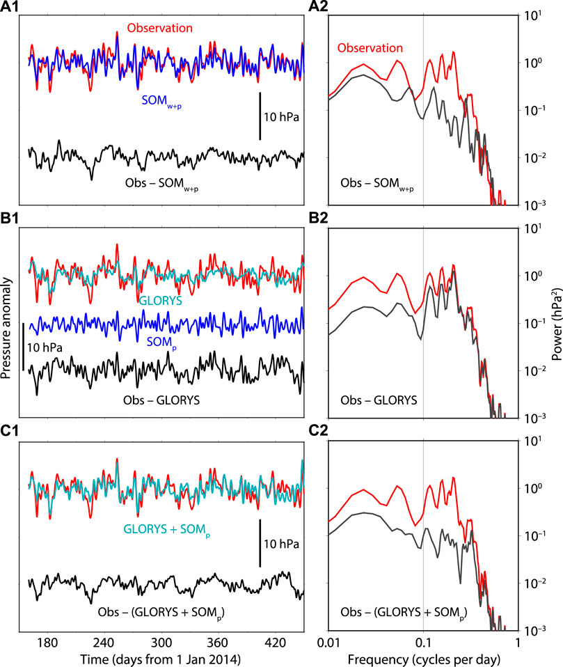
FIGURE 5. Comparison of observed and modeled ocean bottom pressure in time (left) and frequency (right) domains. Red and black indicate observation and residual (observation minus model), respectively. Blue and cyan indicate SOM and GLORYS, respectively. This is an example of LOBS10 (–39.1333°N 178.3132°E) at the Hikurangi Trough.

Observed and Residual Ocean Bottom Pressure at Six Subduction Zones

Comparisons between observed OBP and numerical ocean models are extended to the observation data around the Pacific Ocean (Figure 1; Table 1). Results at representative stations at the six subduction zones are shown in Figures 6–11. Overall results in the respective regions are listed in Table 3. Detailed statistics are found in Supplementary Table S1.

FIGURE 6

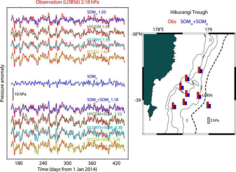
FIGURE 6. Comparisons between observed and modeled ocean bottom pressure at LOBS6 at the Hikurangi Trough. Red indicates the observation at the period of 3–90 days. Blue, dark green, cyan, and light green indicate SOM, HYCOM, GLORYS, and ECCO2, respectively. Upper parts in left panel show comparisons to SOM forced by wind alone (SOM_w), HYCOM, GLORYS, and ECCO2. SOM forced by air pressure alone (SOM_p) (blue) is shown at the center. SOM_p respectively added to SOM_w, HYCOM, GLORYS, and ECCO2 are shown in the lower parts. Root-mean-square amplitude (in hPa) of the observed ocean bottom pressure is shown above the left panel. Root-mean-square amplitudes of residual (observed minus modeled) ocean bottom pressure are attached in the left panel for respective ocean models. Right panel shows the root-mean-square amplitudes of the observed and residual ocean bottom pressure with bar lengths. SOM_w + SOM_p is taken as the representative since this model contributed the best root-mean-square reduction between the models.

FIGURE 7

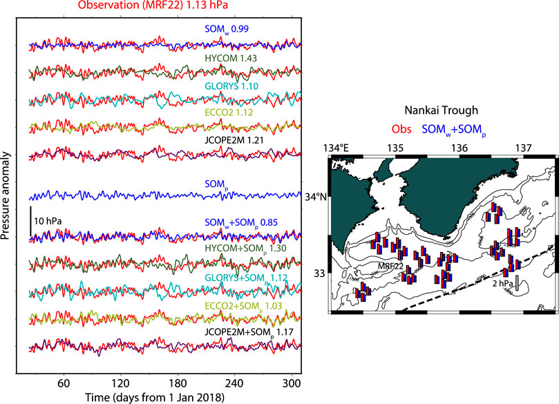
FIGURE 7. Same as Figure 6, but for result at MRF22 at the Nankai Trough. Comparisons with JCOPE2M is added.

FIGURE 8

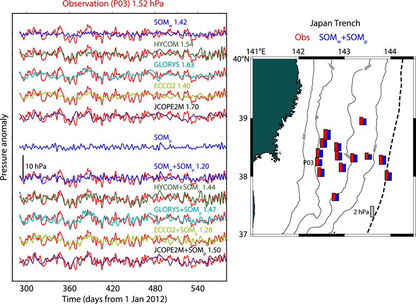
FIGURE 8. Same as Figure 6, but for result at P03 at the Japan Trench. Comparisons with JCOPE2M is added.

FIGURE 9

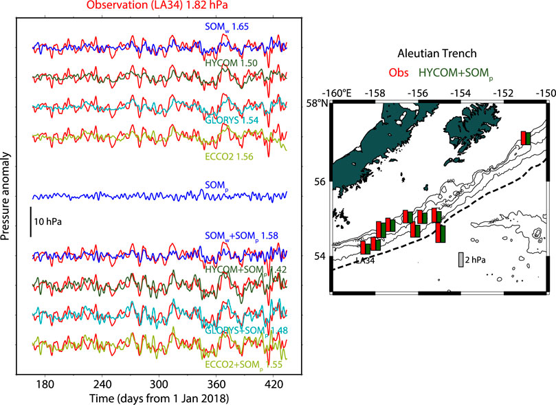
FIGURE 9. Same as Figure 6, but for result at LA34 at the Aleutian Trench.

FIGURE 10

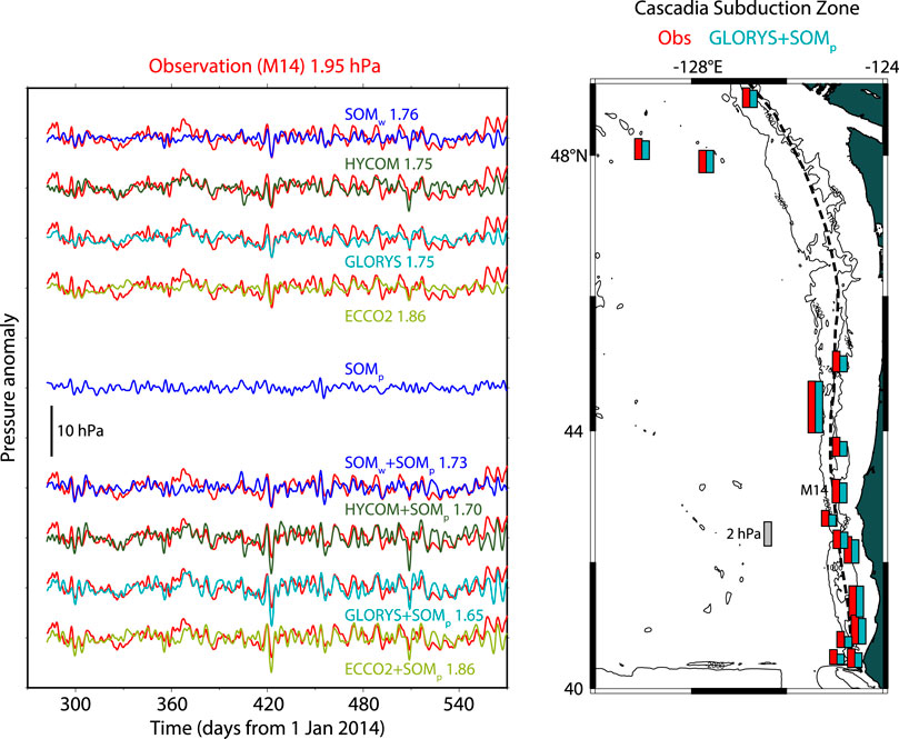
FIGURE 10. Same as Figure 6, but for result at M14 at the Cascadia Subduction Zone.

FIGURE 11

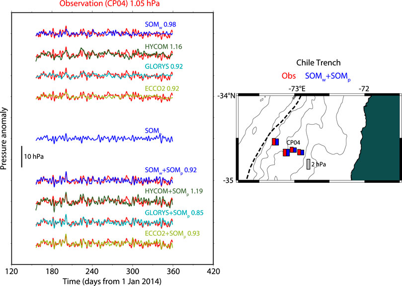
FIGURE 11. Same as Figure 6, but for result at CP04 at the Chile Trench.

TABLE 3

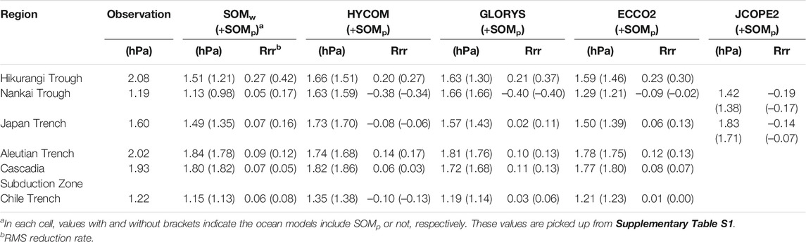
TABLE 3. RMS amplitudes of observations and residual OBP with RMS reduction rate (Eq. 5) using respective ocean models.

The SOM and three multi-layer models (HYCOM, GLORYS, ECCO2) are evaluated for all the observations at the six subduction zones (Hikurangi Trough, Nankai Trough, Japan Trench, Aleutian Trench, Cascadia Subduction Zone, and Chile Trench). In addition to these four global models, JCOPE2M which covers the northwest Pacific Ocean is also tested for the observations around Japan (Nankai Trough and Japan Trench). The OBP data are first compared to that derived from the SOM driven by wind alone (SOM_w), and those derived from the multi-layer models (HYCOM, GLORYS, ECCO2, and JCOPE2M). Subsequently, OBP derived from SOM driven by air pressure alone (SOM_p) is added to the OBP derived from SOM_w, HYCOM, GLORYS, ECCO2, and JCOPE2M, and those are subtracted from the observed OBP data. In this evaluation, we use the RMS reduction rate which is defined at the period of 3–90 days by:

$\text{RMS}\text{reduction}\text{rate}=1-\frac{\text{RMS}\left(\text{Observation}-\text{Model}\right)}{\text{RMS}\left(\text{Observation}\right)}.(5)$

Figure 6 shows the result at the Hikurangi Trough in which the HOBITSS project (Wallace et al., 2016) was carried out. Time series of eight stations from July 2014 to June 2015 were used in the present study. Mean RMS of these time series at the period of 3–90 days was 2.08 hPa. When SOM_w, HYCOM, GLORYS, and ECCO2 were applied, the residual RMS amplitudes were 1.51, 1.66, 1.63, and 1.59 hPa, showing 20–27% RMS reduction rates by the respective models. When SOM_p was added to these models (SOM_w + SOM_p, HYCOM + SOM_p, GLORYS + SOM_p, and ECCO2 + SOM_p), the residual RMS amplitudes were 1.21, 1.51, 1.30, and 1.46 hPa, indicating 27–42% reduction rates from 2.08 hPa. The contribution from SOM_p was shown to be evident with 7–16% reduction rates. SOM_w + SOM_p provided the best RMS reduction of totally 42%, corresponding to a mean correlation coefficient of 0.82 between the observed and modeled OBP (Table 3).

Figure 7 shows the result at the Nankai Trough in which DONET1/2 (Kaneda et al., 2015) is operated. Time series of 45 stations from January 2018 to December 2018 were evaluated. Mean RMS of these time series was 1.19 hPa. When SOM_w, HYCOM, GLORYS, ECCO2, and JCOPE2M were applied, the residual RMS amplitudes were 1.13, 1.63, 1.66, 1.29, and 1.42 hPa. This indicates that SOM_w provided 5% RMS reduction, but other OGCMs hardly contributed to the RMS reduction. When SOM_p was added to these models (SOM_w + SOM_p, HYCOM + SOM_p, GLORYS + SOM_p, ECCO2 + SOM_p, and JCOPE2M + SOM_p), the residual RMS amplitudes were 0.98, 1.59, 1.66, 1.21, and 1.38 hPa. Only SOM_w + SOM_p provided the best RMS reduction of 17%, corresponding to a mean correlation coefficient of 0.58. SOM_p contributed more to the RMS reduction than SOM_w.

Figure 8 shows the result at the Japan Trench in which Tohoku University carried out campaign OBP observations (Hino et al., 2014). Time series of 14 stations from May 2012 to November 2013 were evaluated. Mean RMS of these time series was 1.60 hPa. When SOM_w, HYCOM, GLORYS, ECCO2, and JCOPE2M were applied, the residual RMS amplitudes were 1.49, 1.73, 1.57, 1.50, and 1.83 hPa. SOM_w and ECCO2 provided 6–7% RMS reduction. Other OGCMs hardly contributed to the RMS reduction. When SOM_p was added to these models (SOM_w + SOM_p, HYCOM + SOM_p, GLORYS + SOM_p, ECCO2 + SOM_p, and JCOPE2M + SOM_p), the residual RMS were 1.35, 1.70, 1.43, 1.39, and 1.71 hPa. This shows that SOM_w + SOM_p and ECCO2 + SOM_p provided RMS reduction of 13–16% (correlation coefficient of 0.54), indicating 7–9% contributions from SOM_p. Matsumoto et al. (2006) reported that atmospheric pressure loading was useful to explain OBP variations at offshore northern Japan. A comparable result was confirmed using SOM with substantial number of data.

Figure 9 shows the result at the Aleutian Trench in which the AASCE project (Barcheck et al., 2020) was carried out. Time series of 10 stations from June 2018 to March 2019 were used. Mean RMS of these time series was 2.02 hPa. When SOM_w, HYCOM, GLORYS, and ECCO2 were applied, the residual RMS amplitudes were 1.84, 1.74, 1.81, and 1.78 hPa, indicating 9–14% RMS reduction by the respective models. When SOM_p was added to these models (SOM_w + SOM_p, HYCOM + SOM_p, GLORYS + SOM_p, and ECCO2 + SOM_p), the residual RMS amplitudes were 1.78, 1.68, 1.76, and 1.75 hPa, indicating RMS reduction of 12–17% by the respective models. HYCOM + SOM_p provided the best RMS reduction of 17% (correlation coefficient of 0.55). SOM_p contributed to only 1–3% RMS reduction.

Figure 10 shows the result at the Cascadia Subduction Zone in which the CI project (Toomey et al., 2014) was carried out, and NEPTUNE-Canada (Barnes et al., 2015) is operated. We used time series of 15 stations from October 2012 to June 2013 and from October 2014 to September 2015. Mean RMS of these time series was 1.93 hPa. When SOM_w, HYCOM, GLORYS, and ECCO2, were applied, the residual RMS amplitudes were 1.80, 1.82, 1.72, and 1.77 hPa, indicating 6–11% RMS reduction by the respective models. When SOM_p was added, the residual RMS amplitudes were 1.82, 1.86, 1.68, and 1.80 hPa, indicating that SOM_p contributed to only less than 2% RMS reduction. GLORYS + SOM_p provided the best RMS reduction of 13% (correlation coefficient of 0.51).

Figure 11 shows the result at the Chile Trench in which the Chile PEPPER project (Tréhu et al., 2020) was carried out. Only four time series from May 2012 to March 2013 could be used. Mean RMS was 1.19 hPa. When SOM_w, HYCOM, GLORYS, and ECCO2, were applied, the residual RMS amplitudes were 1.15, 1.35, 1.19, and 1.21 hPa. This indicates <6% RMS reduction by the respective models. When SOM_p was added, the residual RMS amplitudes were 1.13, 1.38, 1.14, and 1.23 hPa. The contribution by SOM_p to the RMS reduction was small (<3%). SOM_w + SOM_p and GLORYS + SOM_p provided RMS reduction of 6–9% (correlation coefficient of 0.51).

The reduction of the residual RMS amplitudes provided by each ocean model with SOM_p is summarized in Figure 12 and Table 3 (see also Supplementary Table S1). The RMS reduction rate of the time series is regarded as a proxy of model accuracy. As shown in Table 3, SOM_w and/or OGCMs performed to represent observations at all the regions with RMS reduction of 5–27%. When SOM_p was added to SOM_w and OGCMs, the RMS reduction rates were up to 8–42% from the original oceanic variations at the period of 3–90 days. At the Hikurangi Trough, the Nankai Trough, and the Japan Trench, SOM_w was relatively accurate (5–27% reduction) compared to other OGCMs, and SOM_p was more effective (additional 9–15% reduction) than other regions. At the Aleutian Trench, HYCOM provided the best RMS reduction of 14%, and SOM_p contributed to additional 3% reduction, with a total reduction of 17%. Other models provided 12–13% RMS reduction. At the Cascadia Subduction Zone, GLORYS provided the best RMS reduction of 11%, and SOM_p contributed to additional 2% reduction, with a total reduction of 13%. At the Chile Trench, SOM_w and GLORYS provided 3–6% RMS reduction, and SOM_p contributed to additional 2–3% reduction.

FIGURE 12

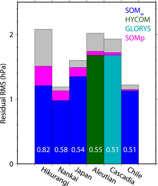
FIGURE 12. Root-mean-square amplitudes of observed and residual ocean bottom pressure at the six subduction zones. Values are calculated as averages over the respective regions, taken from Table 3. White numbers are correlation coefficients corresponding to the root-mean-square reduction rates. Gray and magenta indicate model’s contribution without and with SOM_p, respectively. At the Hikurangi Trough, the Nankai Trough, the Japan Trench, and the Chile Trench, SOM_w + SOM_p is shown as the representative. At the Aleutian Trench, and the Cascadia Subduction Zone, HYCOM + SOM_p, and GLORYS + SOM_p are respectively the representatives.

At the Hikurangi Trough, model representations were relatively good, and RMS reduction rates >20% were found by all the models (Figure 6). SOM was notably accurate as totally 42% RMS reduction including 15% contributions from SOM_p. In the western Pacific regions (Hikurangi Trough, Nankai Trough, and Japan Trench), SOM performed better than other OGCMs to represent OBP. SOM employed the Japanese reanalysis data (JRA-55) as external forcing to drive the ocean, while other ocean models employed US or EU data (Table 2). We speculate the accuracy of JRA-55 may be better than US/EU meteorological data in the western Pacific regions. In the eastern Pacific regions (Aleutian Trench, Cascadia Subduction Zone, and Chile Trench), HYCOM, GLORYS, and ECCO2 were slightly better than SOM or comparable to SOM. Differences of external forcing and/or incorporating vertical layers in OGCMs might contribute to these relative improvements.

As shown in Table 3; and Figure 7, OGCMs unexpectedly performed to increase the residual RMS amplitudes especially at the Nankai Trough. There is a strong western boundary current known as the Kuroshio current that frequently meanders in the vicinity of the Nankai Trough (Qiu and Miao, 2000; Ebuchi and Hanawa, 2003). Due to its meandering and associated mesoscale eddies, OBP also changes with several hPa changes in seasonal or longer time scales (Nagano et al., 2018). When ocean models wrongly represent Kuroshio variations, the residual RMS amplitudes possibly increase. In addition, if residual OBP time series do not correlate well with SOM_p, the subtraction of SOM_p may also increase the residual RMS amplitude, which was found in some cases for the Nankai Trough (Supplementary Table S1). The SOM does not realistically capture the Kuroshio variations, but may weakly represent their features, potentially helping to reduce non-Kuroshio noises in OBP (Figure 12).

Detectability of Seafloor Deformation and Further Root-Mean-Square Reduction

The RMS amplitude of residual OBP time series is crucial in terms of detectability of the seafloor deformation. Based on the result of Figure 12, the evaluations are carried out for the residual RMS amplitude derived from numerical ocean models with and without SOM_p.

At the Nankai Trough and the Chile Trench, the residual RMS was smallest. When SOM_p was added, the residual RMS amplitudes were 1.0–1.1 hPa. As shown in Figures 7 and 11, original RMS amplitudes were also small (1.1–1.2 hPa). The RMS reduction was 16% at the Nankai Trough, and 8% at the Chile Trench. The model accuracy was not so good at the Chile Trench, but the ambient oceanic noise was small there. At the Nankai Trough, possible slow slips were reported using the dense observatories of DONET (Suzuki et al., 2016). When one investigates slow seafloor deformation using OBP observations there, effects of the Kuroshio current should be carefully considered (Nagano et al., 2018). At the Chile Trench, there have only been a few relatively short observations (Tréhu et al., 2020). Future OBP observations at the Chile Trench may enable more detection of small fault slips compared to other regions.

At the Hikurangi Trough and the Japan Trench, the residual RMS amplitudes were both ∼1.5 hPa when SOM_p was not considered. The residual RMS substantially decreased to 1.2–1.3 hPa when SOM_p was added. Original RMS amplitudes were 1.6 hPa at the Japan Trench, and 2.1 hPa at the Hikurangi Trough. The model accuracy of SOM was best at the Hikurangi Trough, although the ambient oceanic components were larger than other regions. The expected detectability is perhaps equivalent between the Hikurangi Trough and the Japan Trench. Previous studies have used OBP observations to identify specific slow slips (Ohta et al., 2012; Ito et al., 2013; Wallace et al., 2016). Recent efforts to improve sensitivities to find transient/ramp steps in OBP records have been increasingly made using ocean models, statistical methods, and/or machine learning in these regions (Hino et al., 2014; Gomberg et al., 2019; Muramoto et al., 2019; He et al., 2020).

At the Aleutian Trench and the Cascadia Subduction Zone, original RMS amplitudes were also large (1.9–2.0 hPa) compared to other regions. Contributions from SOM_p to RMS reduction were small (<0.1 hPa). The residual RMS amplitudes in both the regions were ∼1.7 hPa, being still large when SOM_p was added. Detection of small seafloor deformation may be difficult in these regions compared to other regions, due to larger ambient oceanic noises and lack of model accuracy. By using a local ocean state estimation based on HYCOM boundary condition, Fredrickson et al. (2019) carried out an effort to reduce RMS of OBP observations at the Cascadia Subduction Zone partially same as those used in our study, and they also had obtained results quantitatively similar to our study.

The inverted barometer response of sea level has often been assumed to be robust for periods greater than a few days, indicating SOM_p has been often negligible. However, the results shown above suggested that SOM_p was mostly non-negligible and provided 2–15% RMS reduction in OBP in time scales of days to months (3–90 days) at the six subduction zones. Note that mean air pressure at the sea level over the global ocean has seasonal amplitudes of less than a few hPa (Ponte, 1993; Wunsch and Stammer, 1997). Seasonal changes of the total freshwater volume in the ocean may contribute to <1 hPa changes in OBP over the global ocean (Ponte et al., 2007). Sea level response to atmospheric Rossby-Haurwitz waves at a period of 5 days significantly deviates from the inverted barometer (Hirose et al., 2001; Mathers and Woodworth, 2004). Other mechanisms of departure from inverted barometer have been investigated as well (Stepanov and Hughes, 2006). The deviations from the inverted barometer (i.e., SOM_p) should be taken into account even in deep-sea regions when OBP observations are used to find small signals (<a few centimeters) of slow seafloor deformation.

We utilized a single-layer ocean model of Inazu et al. (2012) to provide SOM_p. Better representations of the oceanic variations induced by air pressure may be obtained by using OGCMs that represent realistic ocean interior. According to Ponte and Vinogradov (2007), air-pressure-induced OBP involves up to a 20% difference between stratified and non-stratified oceans. Comprehensive modeling including self-attraction and loading effects on seafloor (Stepanov and Hughes, 2004; Vinogradova et al., 2015) may help to improve representations of OBP variations. In addition to these reasonable ocean dynamics, boundary conditions of bathymetry and meteorological data should be also accurate to represent more realistic oceanic variations. Digital elevation models with global bathymetry are still going to be updated (Tozer et al., 2019). SOM employed the Japanese meteorological reanalysis data (JRA-55) which might be relatively accurate at Asia and western Pacific, compared to other regions. According to the result of Figure 12, substantial improvements at the Aleutian Trench, the Cascadia Subduction Zone, and the Chile Trench are expected if the accuracy of the meteorological data can be improved there.

Gomberg et al. (2019) and Fredrikson et al. (2019) respectively utilized local OGCMs with HYCOM-based boundary conditions to reduce RMS amplitudes of OBP observations for slow slip detections. The RMS reduction might be more efficient if air pressure to drive the ocean is incorporated into their ocean models. Recently, Androsov et al. (2020) showed that atmospheric pressure loading has a role to improve correlation between observed and modeled OBP of both daily and monthly time scales at the Southern Ocean. When air-pressure induced components (eg, SOM_p) become widely available in addition to wind-driven OGCMs, such ocean models will become more useful for marine geophysics applications.

In the present study, we used a band-pass filter to compare extracted oceanic signals as well as to systematically remove long-term drift in OBP data at several subduction zones. However, band-pass filtering has potential to obscure a ramp change which may correspond to a slow seafloor deformation. When one tries to isolate slow seafloor deformation, band-pass filtering is not appropriate in most cases, and long-term drift should be carefully estimated and removed using other approaches. In this paper, we have focused on accurate estimation of oceanic variations. Note that if oceanic variations are better estimated especially at long periods, this will also help to better estimate long-term drift component. Drift estimation has been conventionally done by fitting a function (typically exponential + linear) to de-tided OBP time series (Eble et al., 1989; Polster et al., 2009). However, better drift estimation is expected by fitting the function to the OBP residual after removing both tides and longer-period non-tidal oceanic variations. Improved drift estimation will contribute to better detectability of seafloor deformation.

Summary

OBP observation data at six subduction zones around the Pacific Ocean were investigated to improve detectability of slow seafloor deformation signals. Numerical ocean models were used to reduce RMS of oceanic components in OBP records at a period of 3–90 days. The ocean models included HYCOM, GLORYS, ECCO2, JCOPE2M, and SOM. The RMS reduction rate using Eq. 5 was used to measure accuracy of these models. The RMS reduction of 5–27% were provided using these models at the six regions. Departure from an inverted barometer response was calculated using SOM with atmospheric pressure loading, which was not considered in the currently available OGCMs. This component was effective with additional RMS reduction of 9–15% at the Hikurangi Trough, the Nankai Trough, and the Japan Trench. But the component was not so effective with only <3% RMS reduction in other regions (Table 3; Figure 12).

The RMS amplitudes of the residual OBP time series can be a proxy for detectability of slow seafloor deformation. The residual RMS amplitude depends on regions and accuracy of ocean models. As a result, the residual RMS amplitudes were 1.0–1.1 hPa at the Nankai Trough and the Chile Trench, 1.2–1.4 hPa at the Hikurangi Trough and the Japan Trench, and 1.7–1.8 hPa at the Aleutian Trench and the Cascadia Subduction Zone (Table 3; Figure 12). Detectability of slow seafloor deformation is expected to be better in regions with smaller residual RMS amplitudes.

These were the results for the data at specific observation periods. However, we expect that comparable features of the RMS reduction will be obtained for other data periods at the respective regions. Although there will be room to improve model accuracy, the present study evaluated the utility of currently available ocean models to reduce oceanic noise in OBP observations for detections of slow seafloor deformation in subduction zones. It is still not so easy to detect slow seafloor deformation of less than a few centimeters from single OBP station time series (Inazu et al., 2012; Muramoto et al., 2019). Further efforts will be suitably combined by differentiating time series and/or statistical method using a number of stations (Ito et al., 2013; Ariyoshi et al., 2014; Hino et al., 2014; Wallace et al., 2016).

Improving accuracy of numerical ocean models with data assimilation is essentially useful to accurately estimate and remove oceanic noises at each station. This study showed that OGCMs did not always perform better than SOM, and OBP changes induced by atmospheric pressure loading should be incorporated to enhance the representations of OBP variations at the period of 3–90 days. Improvements of accuracy of boundary conditions including external force (e.g, meteorological data) are also required as well as reasonable ocean dynamics for more precise estimation of OBP. Integrated approaches from oceanography and solid earth science are indispensable for improving future seafloor geodesy.

Data Availability Statement

Most of the OBP observation data used were provided by the Ocean Bottom Seismograph Instrument Pool (http://www.obsip.org) which is funded by the National Science Foundation. The OBP observation data of the DONET1/2 observatory are available via the database of the National Research Institute for Earth Science and Disaster Resilience (https://doi.org/10.17598/nied.0008). The OBP observation data of NEPTUNE Canada are available via the database of the Ocean Networks Canada (http://doi.org/10.17616/R3SK62). Ocean reanalysis datasets are available via respective data centers/servers of HYCOM (https://www.hycom.org/dataserver), GLORYS (https://resources.marine.copernicus.eu/?option=com_csw&task=results), ECCO2 (https://ecco-group.org/products.htm), and JCOPE2M (http://www.jamstec.go.jp/jcope/htdocs/e/distribution/index.html).

Author Contributions

Both authors designed this research, carried out analyses, discussed the results, and wrote the paper.

Funding

This study was supported by JSPS KAKENHI Grant number 18K04654.

Conflict of Interest

The authors declare that the research was conducted in the absence of any commercial or financial relationships that could be construed as a potential conflict of interest.

The handling editor declared a past co-authorship with one of the authors (DI).

Acknowledgments

We appreciate Prof. Ryota Hino, and Associate Prof. Yusaku Ohta of Tohoku University for kindly providing OBP data at the Japan Trench. Dr. Narumi Takahashi, Dr. Takeshi Nakamura, and Dr. Tatsuya Kubota of the National Research Institute for Earth Science and Disaster Resilience, Japan, kindly helped us to obtain OBP data of the DONET1/2 observatory. We thank Dr. Ruochao Zhang of the Japan Agency for Marine-Earth Science and Technology for providing comprehensive dataset of JCOPE2M. Discussion with Mr. Tomoya Muramoto of the National Institute of Advanced Industrial Science and Technology, Japan, was useful for analyzing OBP at the Hikurangi Trough. Comments from two reviewers and those from Dr. Laura Wallace, Guest Editor for the special issue, greatly improved the manuscript.

Supplementary Material

The Supplementary Material for this article can be found online at: https://www.frontiersin.org/articles/10.3389/feart.2020.598270/full#supplementary-material.

References

Androsov, A., Boebel, O., Schröter, J., Danilov, S., Macrander, A., and Ivanciu, I. (2020). Ocean bottom pressure variability: Can it be reliably modeled? J. Geophys. Res. Oceans 125, e2019JC015469. doi:10.1029/2019JC015469

CrossRef Full Text | Google Scholar

Aoi, S., Asano, Y., Kunugi, T., Kimura, T., Uehira, K., Takahashi, N., et al. (2020). MOWLAS: NIED observation network for earthquake, tsunami and volcano. Earth Planets Space 72, 126. doi:10.1186/s40623-020-01250-x

CrossRef Full Text | Google Scholar

Ariyoshi, K., Nakata, R., Matsuzawa, T., Hino, R., Hori, T., Hasegawa, A., et al. (2014). The detectability of shallow slow earthquakes by the Dense Oceanfloor Network system for Earthquakes and Tsunamis (DONET) in Tonankai district, Japan. Mar. Geophys. Res. 35, 295–310. doi:10.1007/s11001-013-9192-6

CrossRef Full Text | Google Scholar

Baba, S., Takeo, A., Obara, K., Matsuzawa, T., and Maeda, T. (2020). Comprehensive detection of very low frequency earthquakes off the Hokkaido and Tohoku Pacic coasts, Northeastern Japan. J. Geophys. Res. Solid Earth. 125, e2019JB017988. doi:10.1029/2019JB017988

CrossRef Full Text | Google Scholar

Baba, T., Hirata, K., Hori, T., and Sakaguchi, H. (2006). Offshore geodetic data conducive to the estimation of the afterslip distribution following the 2003 Tokachi-oki earthquake. Earth Planet Sci. Lett. 241, 281–292. doi:10.1016/j.epsl.2005.10.019

CrossRef Full Text | Google Scholar

Bailey, K., DiVeglio, C., and Welty, A. (2014). “An examination of the June 2013 East Coast meteotsunami captured by NOAA observing systems.” in NOAA Technical Report, NOS CO-OPS 079, 42.

Google Scholar

Barcheck, G., Abers, G. A., Adams, A. N., Bécel, A., Collins, J., Gaherty, J. B., et al. (2020). The Alaska amphibious community seismic experiment. Seismol. Res. Lett. 91, 3054–3063. doi:10.1785/0220200189

CrossRef Full Text | Google Scholar

Barnes, C. R., Best, M. M. R., Johnson, F. R., and Pirenne, B. (2015). “NEPTUNE Canada: installation and initial operation of the world’s first regional cabled ocean observatory.” in Seafloor observatories. (Berlin, Germany: Springer Praxis Books. Springer), 415–438. doi:10.1007/978-3-642-11374-1_16

CrossRef Full Text | Google Scholar

Beardsley, R. C., Mofjeld, H., Wimbush, M., Flagg, C. N., and Vermersch, J. A. (1977). Ocean tides and weather‐induced bottom pressure fluctuations in the middle‐Atlantic bight. J. Geophys. Res. Oceans and Atmospheres 82, 3175–3182. doi:10.1029/JC082i021p03175

CrossRef Full Text | Google Scholar

Bird, P. (2003). An updated digital model of plate boundaries. Geochem. Geophys. Geosyst. 4, 1027. doi:10.1029/2001GC000252

CrossRef Full Text | Google Scholar

Chadwick, W. W., Nooner, S. L., Butterfield, D. A., and Lilley, M. D. (2012). Seafloor deformation and forecasts of the April 2011 eruption at axial seamount. Nat. Geosci. 5, 474–477. doi:10.1038/ngeo1464

CrossRef Full Text | Google Scholar

Chereskin, T. K., Donohue, K. A., Watts, D. R., Tracey, K. L., Firing, Y. L., and Cutting, A. L. (2009). Strong bottom currents and cyclogenesis in Drake Passage. Geophys. Res. Lett. 36, L23602. doi:10.1029/2009GL040940

CrossRef Full Text | Google Scholar

Cummings, J. A., and Smedstad, O. M. (2013). “Variational data analysis for the global ocean.” in Data assimilation for atmospheric, oceanic and hydrologic applications. (Berlin, Germany: Springer-Verlag), 303–343. doi:10.1007/978-3-642-35088-7_13

CrossRef Full Text | Google Scholar

Davis, E. E., Villinger, H., and Sun, T. (2015). Slow and delayed deformation and uplift of the outermost subduction prism following ETS and seismogenic slip events beneath Nicoya Peninsula, Costa Rica. Earth Planet Sci. Lett. 410, 117–127. doi:10.1016/j.epsl.2014.11.015

CrossRef Full Text | Google Scholar

Donohue, K. A., Watts, D. R., Tracey, K. L., Greene, A. D., and Kennelly, M. (2010). Mapping circulation in the Kuroshio Extension with an array of current and pressure recording inverted echo sounders. J. Atmos. Ocean. Technol. 27, 507–527. doi:10.1175/2009JTECHO686.1

CrossRef Full Text | Google Scholar

Eble, M. C., Gonzalez, F. I., Mattens, D. M., and Milburn, H. B. (1989). “Instrumentation, field operations, and data processing for PMEL deep ocean bottom pressure measurements.” in NOAA technical memorandum ERL PMEL. (Washington, DC: US Government Printing Office), 89, 71.

Google Scholar

Eble, M. C., and Gonzalez, F. I. (1991). Deep-ocean bottom pressure measurements in the northeast Pacific. J. Atmos. Oceanic Technol. 8, 221–233. doi:10.1175/1520-0426(1991)008<0221:DOBPMI>2.0.CO;2

CrossRef Full Text | Google Scholar

Ebuchi, N., and Hanawa, K. (2003). Influence of mesoscale eddies on variations of the Kuroshio path south of Japan. J. Oceanogr. 59, 25–36. doi:10.1023/A:1022856122033

CrossRef Full Text | Google Scholar

Egbert, G. D., and Erofeeva, S. Y. (2002). Efficient inverse modeling of barotropic ocean tides. J. Atmos. Oceanic Technol. 19, 183–204. doi:10.1175/1520-0426(2002)019<0183:EIMOBO>2.0.CO;2

CrossRef Full Text | Google Scholar

Emery, W. J., and Thomson, R. E. (2001). Data analysis methods in physical oceanography. Second and Revised Edn. Amsterdam, Netherlands: Elsevier Science, 638. doi:10.1016/B978-0-444-50756-3.X5000-X

CrossRef Full Text | Google Scholar

Filloux, J. H. (1971). Deep-sea tide observations from the northeastern Pacific. Deep-Sea Res. 18, 275–284. doi:10.1016/0011-7471(71)90118-5

CrossRef Full Text | Google Scholar

Filloux, J. H. (1983). Pressure fluctuations on the open-ocean floor off the Gulf of California: Tides, earthquakes, tsunamis. J. Phys. Oceanogr. 13, 783–796. doi:10.1175/1520-0485(1983)013<0783:PFOTOO>2.0.CO;2

CrossRef Full Text | Google Scholar

Fofonoff, N. P., and Millard, R. C. (1983). “Algorithms for the computation of fundamental properties of seawater,” UNESCO Technical Papers in Marine Sciences; 44. (Paris, France: UNESCO), 53.

Google Scholar

Fox, C. G. (1999). In situ ground deformation measurements from the summit of Axial Volcano during the 1998 volcanic episode. Geophys. Res. Lett. 26, 3437–3440. doi:10.1029/1999GL900491

CrossRef Full Text | Google Scholar

Fredrickson, E. K., Wilcock, W. S. D., Schmidt, D. A., MacCready, P., Roland, E., Kurapov, A. L., et al. (2019). Optimizing sensor configurations for the detection of slow-slip earthquakes in seafloor pressure records, using the Cascadia Subduction Zone as a case study. J. Geophys. Res. Solid Earth 124, 13504–13531. doi:10.1029/2019JB018053

CrossRef Full Text | Google Scholar

Gill, A. E. (1982). “Adjustment under gravity of a density-stratified fluid,” in Atmosphere-ocean dynamics. (San Diego, CA: Academic Press), 117–188. doi:10.1016/S0074-6142(08)60031-5

CrossRef Full Text | Google Scholar

Gomberg, J., Hautala, S., Johnson, P., and Chiswell, S. (2019). Separating sea and slow slip signals on the seafloor. J. Geophys. Res. Solid Earth 124, 13486–13503. doi:10.1029/2019JB018285

CrossRef Full Text | Google Scholar

He, B., Wei, M., Watts, D. R., and Shen, Y. (2020). Detecting slow slip events from seafloor pressure data using machine learning. Geophys. Res. Lett. 47, e2020GL087579. doi:10.1029/2020GL087579

CrossRef Full Text | Google Scholar

Hino, R., Ii, S., Iinuma, T., and Fujimoto, H. (2009). Continuous long-term seafloor pressure observation for detecting slow-slip interplate events in Miyagi-Oki on the landward Japan Trench slope. J. Disaster Res. 4, 72–82. doi:10.20965/jdr.2009.p0072

CrossRef Full Text | Google Scholar

Hino, R., Inazu, D., Ohta, Y., Ito, Y., Suzuki, S., Iinuma, T., et al. (2014). Was the 2011 Tohoku-Oki earthquake preceded by aseismic preslip? Examination of seafloor vertical deformation data near the epicenter. Mar. Geophys. Res. 35, 181–190. doi:10.1007/s11001-013-9208-2

CrossRef Full Text | Google Scholar

Hirata, K., Aoyagi, M., Mikada, H., Kawaguchi, K., Kaiho, Y., Iwase, R., et al. (2002). Real-time geophysical measurements on the deep seafloor using submarine cable in the southern Kurile subduction zone. IEEE J. Ocean. Eng. 27, 170–181. doi:10.1109/joe.2002.1002471

CrossRef Full Text | Google Scholar

Hirose, H., and Obara, K. (2005). Repeating short- and long-term slow slip events with deep tremor activity around the Bungo channel region, southwest Japan. Earth Planets Space 57, 961–972. doi:10.1186/BF03351875

CrossRef Full Text | Google Scholar

Hirose, N., Fukumori, I., and Ponte, R. M. (2001). A non‐isostatic global sea level response to barometric pressure near 5 days. Geophys. Res. Lett. 28, 2441–2444. doi:10.1029/2001GL012907

CrossRef Full Text | Google Scholar

Inazu, D., Hino, R., and Fujimoto, H. (2012). A global barotropic ocean model driven by synoptic atmospheric disturbances for detecting seafloor vertical displacements from in situ ocean bottom pressure measurements. Mar. Geophys. Res. 33, 127–148. doi:10.1007/s11001-012-9151-7

CrossRef Full Text | Google Scholar

Inazu, D., and Hino, R. (2011). Temperature correction and usefulness of ocean bottom pressure data from cabled seafloor observatories around Japan for analyses of tsunamis, ocean tides, and low-frequency geophysical phenomena. Earth Planets Space 63, 1133–1149. doi:10.5047/eps.2011.07.014

CrossRef Full Text | Google Scholar

Inazu, D., Hirose, N., Kizu, S., and Hanawa, K. (2006). Zonally asymmetric response of the Japan Sea to synoptic pressure forcing. J. Oceanogr. 62, 909–916. doi:10.1007/s10872-006-0108-9

CrossRef Full Text | Google Scholar

Inazu, D., and Saito, T. (2016). Global tsunami simulation using a grid rotation transformation in a latitude–longitude coordinate system. Nat. Hazards 80, 759–773. doi:10.1007/s11069-015-1995-0

CrossRef Full Text | Google Scholar

Irish, J. D., and Snodgrass, F. E. (1972). Quartz crystals as multipurpose oceanographic sensors—I. Pressure. Deep-Sea Res. 19, 165–169. doi:10.1016/0011-7471(72)90049-6

CrossRef Full Text | Google Scholar

Ito, Y., Hino, R., Kido, M., Fujimoto, H., Osada, Y., Inazu, D., et al. (2013). Episodic slow slip events in the Japan subduction zone before the 2011 Tohoku-Oki earthquake. Tectonophysics 600, 14–26. doi:10.1016/j.tecto.2012.08.022

CrossRef Full Text | Google Scholar

Ito, Y., Tsuji, T., Osada, Y., Kido, M., Inazu, D., Hayashi, Y., et al. (2011). Frontal wedge deformation near the source region of the 2011 Tohoku‐Oki earthquake. Geophys. Res. Lett. 38, L00G05. doi:10.1029/2011GL048355

CrossRef Full Text | Google Scholar

Itoh, Y., Nishimura, T., Ariyoshi, K., and Matsumoto, H. (2019). Interplate slip following the 2003 Tokachi‐oki earthquake from ocean bottom pressure gauge and land GNSS data. J. Geophys. Res. Solid Earth 124, 4205–4230. doi:10.1029/2018JB016328

CrossRef Full Text | Google Scholar

Kajikawa, H., and Kobata, T. (2019). Different long-term characteristics of hydraulic pressure gauges under constant pressure applications. Acta IMEKO 8, 19–24. doi:10.21014/acta_imeko.v8i3.665

CrossRef Full Text | Google Scholar

Kaneda, Y., Kawaguchi, K., Araki, E., Matsumoto, H., Nakamura, T., Kamiya, S., et al. (2015). “Development and application of an advanced ocean floor network system for megathrust earthquakes and tsunamis,” in Seafloor observatories. (Berlin, Germany: Springer Praxis Books. Springer), 643–662. doi:10.1007/978-3-642-11374-1_25

CrossRef Full Text | Google Scholar

Kobayashi, S., Ota, Y., Harada, Y., Ebita, A., Moriya, M., Onoda, H., et al. (2015). The JRA-55 Reanalysis: general specifications and basic characteristics. J. Meteorol. Soc. Jpn. 93, 5–48. doi:10.2151/jmsj.2015-001

Google Scholar

Kubota, T., Chikasada, N. Y., Hino, R., Ohta, Y., and Otsuka, H. (2020). “Preliminary assessment of quality of the S-net long-term ocean bottom pressure observation in the northern part of the Japan Trench for detecting crustal deformation,” in JpGU-AGU Joint Meeting, Virtual Meeting, SCG66.

CrossRef Full Text | Google Scholar

Kubota, T., Hino, R., Inazu, D., and Suzuki, S. (2019). Fault model of the 2012 doublet earthquake, near the up-dip end of the 2011 Tohoku-Oki earthquake, based on a near-field tsunami: implications for intraplate stress state. Prog. Earth Planet. Sci. 6, 67. doi:10.1186/s40645-019-0313-y

CrossRef Full Text | Google Scholar

Kubota, T., Saito, T., Suzuki, W., and Hino, R. (2017). Estimation of seismic centroid moment tensor using ocean bottom pressure gauges as seismometers. Geophys. Res. Lett. 44, 10907–10915. doi:10.1002/2017GL075386

CrossRef Full Text | Google Scholar

Kubota, T., Suzuki, W., Nakamura, T., Chikasada, N. Y., Aoi, S., Takahashi, N., et al. (2018). Tsunami source inversion using time-derivative waveform of offshore pressure records to reduce effects of non-tsunami components. Geophys. J. Int. 215, 1200–1214. doi:10.1093/gji/ggy345

CrossRef Full Text | Google Scholar

Lellouche, J.-M., Greiner, E., Le Galloudec, O., Garric, G., Regnier, C., Drevillon, M., et al. (2018). Recent updates to the Copernicus Marine Service global ocean monitoring and forecasting real-time 1/12 high-resolution system. Ocean Sci. 14, 1093–1126. doi:10.5194/os-14-1093-2018

CrossRef Full Text | Google Scholar

Mathers, E. L., and Woodworth, P. L. (2004). A study of departures from the inverse‐barometer response of sea level to air‐pressure forcing at a period of 5 days. Q. J. R. Meteorol. Soc. 130, 725–738. doi:10.1256/qj.03.46

CrossRef Full Text | Google Scholar

Matsumoto, K., Sato, T., Fujimoto, H., Tamura, Y., Nishino, M., Hino, R., et al. (2006). Ocean bottom pressure observation off Sanriku and comparison with ocean tide models, altimetry, and barotropic signals from ocean models. Geophys. Res. Lett. 33, L16602. doi:10.1029/2006GL026706

Google Scholar

Menemenlis, D., Campin, J.-M., Heimbach, P., Hill, C., Lee, T., Nguyen, A., et al. (2008). ECCO2: high resolution global ocean and sea ice data synthesis. Mercator Ocean Quarterly Newsletter 31, 13–21.

CrossRef Full Text | Google Scholar

Miyazawa, Y., Varlamov, S. M., Miyama, T., Guo, X., Hihara, T., Kiyomatsu, K., et al. (2017). Assimilation of high-resolution sea surface temperature data into an operational nowcast/forecast system around Japan using a multi-scale three-dimensional variational scheme. Ocean Dynam. 67, 713–728. doi:10.1007/s10236-017-1056-1

CrossRef Full Text | Google Scholar

Mofjeld, H. O., González, F. I., Eble, M. C., and Newman, J. C. (1995). Ocean tides in the continental margin off the pacific northwest shelf. J. Geophys. Res. Oceans 100, 10789–10800. doi:10.1029/95JC00687

CrossRef Full Text | Google Scholar

Mofjeld, H. O., González, F. I., and Eble, M. C. (1996). Subtidal bottom pressure observed at Axial Seamount in the northeastern continental margin of the Pacific Ocean. J. Geophys. Res. Oceans 101, 16381–16390. doi:10.1029/96JC01451

PubMed Abstract | CrossRef Full Text | Google Scholar

Munk, W. H., and Zetler, B. D. (1967). Deep-sea tides: a problem. Science 158, 884–886. doi:10.1126/science.158.3803.884

CrossRef Full Text | Google Scholar

Munk, W., Snodgrass, F., and Wimbush, M. (1970). Tides off‐shore: transition from California coastal to deep‐sea waters. Geophys. Astrophys. Fluid Dynam. 1, 161–235. doi:10.1080/03091927009365772

CrossRef Full Text | Google Scholar

Muramoto, T., Ito, Y., Inazu, D., Wallace, L. M., Hino, R., Suzuki, S., et al. (2019). Seaoor crustal deformation on ocean bottom pressure records with nontidal variability corrections: application to Hikurangi margin, New Zealand. Geophys. Res. Lett. 46, 303–310. doi:10.1029/2018GL080830

CrossRef Full Text | Google Scholar

Nagano, A., Hasegawa, T., Matsumoto, H., and Ariyoshi, K. (2018). Bottom pressure change associated with the 2004–2005 large meander of the Kuroshio south of Japan. Ocean Dynam. 68, 847–865. doi:10.1007/s10236-018-1169-1

CrossRef Full Text | Google Scholar

Niiler, P. P., Filloux, J., Liu, W. T., Samelson, R. M., Paduan, J. D., and Paulson, C. A. (1993). Wind-forced variability of the deep eastern North Pacific: observations of seafloor pressure and abyssal currents. J. Geophys. Res. Oceans 98, 22589–22602. doi:10.1029/93JC01288

CrossRef Full Text | Google Scholar

Nosov, M. A., and Kolesov, S. V. (2007). Elastic oscillations of water column in the 2003 Tokachi-oki tsunami source: in-situ measurements and 3-D numerical modelling. Nat. Hazards Earth Syst. Sci. 7, 243–249. doi:10.5194/nhess-7-243-2007

CrossRef Full Text | Google Scholar

Nosov, M., Karpov, V., Kolesov, S., Sementsov, K., Matsumoto, H., and Kaneda, Y. (2018). Relationship between pressure variations at the ocean bottom and the acceleration of its motion during a submarine earthquake. Earth Planets Space 70, 100. doi:10.1186/s40623-018-0874-9

CrossRef Full Text | Google Scholar

Nowroozi, A. A., Kuo, J., and Ewing, M. (1969). Solid earth and oceanic tides recorded on the ocean floor off the coast of northern California. J. Geophys. Res. Solid Earth 74, 605–614. doi:10.1029/JB074i002p00605

CrossRef Full Text | Google Scholar

Ohta, Y., Hino, R., Inazu, D., Ohzono, M., Ito, Y., Mishina, M., et al. (2012). Geodetic constraints on afterslip characteristics following the March 9, 2011, Sanriku-Oki earthquake, Japan. Geophys. Res. Lett. 39, L16304. doi:10.1029/2012GL052430

CrossRef Full Text | Google Scholar

Park, J.-H., Donohue, K. A., Watts, D. R., and Rainville, L. (2010). Distribution of deep near-inertial waves observed in the Kuroshio Extension. J. Oceanogr. 66, 709–717. doi:10.1007/s10872-010-0058-0

CrossRef Full Text | Google Scholar

Park, J.-H., Watts, D. R., Donohue, K. A., and Jayne, S. R. (2008). A comparison of in situ bottom pressure array measurements with GRACE estimates in the Kuroshio Extension. Geophys. Res. Lett. 35, L17601. doi:10.1029/2008GL034778

Google Scholar

Paros, J. M. (2017). Seismic + oceanic sensors (SOS) for ocean disasters and geodesy. Redmond, WA: Paroscientific, Inc.

CrossRef Full Text | Google Scholar

Peralta-Ferriz, C., Morison, J. H., and Wallace, J. M. (2016). Proxy representation of Arctic ocean bottom pressure variability: bridging gaps in GRACE observations. Geophys. Res. Lett. 43, 9183–9191. doi:10.1002/2016GL070137

CrossRef Full Text | Google Scholar

Polster, A., Fabian, M., and Villinger, H. (2009). Effective resolution and drift of Paroscientific pressure sensors derived from long‐term seafloor measurements. Geochem. Geophys. Geosyst. 10, Q08008. doi:10.1029/2009GC002532

CrossRef Full Text | Google Scholar

Ponte, R. M. (2006). Oceanic response to surface loading effects neglected in volume-conserving models. J. Phys. Oceanogr. 36, 426–434. doi:10.1175/JPO2843.1

CrossRef Full Text | Google Scholar

Ponte, R. M., Quinn, K. J., Wunsch, C., and Heimbach, P. (2007). A comparison of model and GRACE estimates of the large‐scale seasonal cycle in ocean bottom pressure. Geophys. Res. Lett. 34, L09603. doi:10.1029/2007GL029599

CrossRef Full Text | Google Scholar

Ponte, R. M. (1993). Variability in a homogeneous global ocean forced by barometric pressure. Dynam. Atmos. Oceans 18, 209–234. doi:10.1016/0377-0265(93)90010-5

CrossRef Full Text | Google Scholar

Ponte, R. M., and Vinogradov, S. V. (2007). Effects of stratification on the large-scale ocean response to barometric pressure. J. Phys. Oceanogr. 37, 245–258. doi:10.1175/JPO3010.1

CrossRef Full Text | Google Scholar

Qiu, B., and Miao, W. (2000). Kuroshio path variations south of Japan: Bimodality as a self-sustained internal oscillation. J. Phys. Oceanogr. 30, 2124–2137. doi:10.1175/1520-0485(2000)030<2124:KPVSOJ>2.0.CO;2

CrossRef Full Text | Google Scholar

Rabinovich, A. B., and Eblé, M. C. (2015). Deep-ocean measurements of tsunami waves. Pure Appl. Geophys. 172, 3281–3312. doi:10.1007/s00024-015-1058-1

PubMed Abstract | CrossRef Full Text | Google Scholar

Ruiz, S., Metois, M., Fuenzalida, A., Ruiz, J., Leyton, F., Grandin, R., et al. (2014). Intense foreshocks and a slow slip event preceded the 2014 Iquique Mw 8.1 earthquake. Science 345, 1165–1169. doi:10.1126/science.1256074

CrossRef Full Text | Google Scholar

Sasagawa, G., Cook, M. J., and Zumberge, M. A. (2016). Drift-corrected seaoor pressure observations of vertical deformation at Axial Seamount 2013-2014. Earth Space Sci. 3, 381–385 doi:10.1002/2016EA000190

CrossRef Full Text | Google Scholar

Sato, T., Hasegawa, S., Kono, A., Shiobara, H., Yagi, T., Yamada, T., et al. (2017). Detection of vertical motion during a slow-slip event off the Boso Peninsula, Japan, by ocean bottom pressure gauges. Geophys. Res. Lett. 44, 2710–2715. doi:10.1002/2017GL072838

CrossRef Full Text | Google Scholar

Siegismund, F., Romanova, V., Köhl, A., and Stammer, D. (2011). Ocean bottom pressure variations estimated from gravity, nonsteric sea surface height and hydrodynamic model simulations. J. Geophys. Res. Oceans 116, C07021. doi:10.1029/2010JC006727

CrossRef Full Text | Google Scholar

Stepanov, V. N., and Hughes, C. W. (2004). Parameterization of ocean self-attraction and loading in numerical models of the ocean circulation. J. Geophys. Res. Oceans 109, C03037. doi:10.1029/2003JC002034

CrossRef Full Text | Google Scholar

Stepanov, V. N., and Hughes, C. W. (2006). Propagation of signals in basin‐scale ocean bottom pressure from a barotropic model. J. Geophys. Res. Oceans 111, C12002. doi:10.1029/2005JC003450

CrossRef Full Text | Google Scholar

Suzuki, K., Nakano, M., Takahashi, N., Hori, T., Kamiya, S., Araki, E., et al. (2016). Synchronous changes in the seismicity rate and ocean-bottom hydrostatic pressures along the Nankai trough: a possible slow slip event detected by the Dense Oceanfloor Network system for Earthquakes and Tsunamis (DONET). Tectonophysics 680, 90–98. doi:10.1016/j.tecto.2016.05.012

CrossRef Full Text | Google Scholar

Tamura, Y., Sato, T., Ooe, M., and Ishiguro, M. (1991). A procedure for tidal analysis with a Bayesian information criterion. Geophys. J. Int. 104, 507–516. doi:10.1111/j.1365-246X.1991.tb05697.x

CrossRef Full Text | Google Scholar

Tanaka, S., Matsuzawa, T., and Asano, Y. (2019). Shallow low‐frequency tremor in the northern Japan Trench subduction zone. Geophys. Res. Lett. 46, 5217–5224. doi:10.1029/2019GL082817

CrossRef Full Text | Google Scholar

Toomey, D. R., Allen, R. M., Barclay, A. H., Bell, S. W., Bromirski, P. D., Carlson, R. L., et al. (2014). The Cascadia Initiative: a sea change in seismological studies of subduction zones. Oceanography 27, 138–150. doi:10.5670/oceanog.2014.49

CrossRef Full Text | Google Scholar

Tozer, B., Sandwell, D. T., Smith, W. H. F., Olson, C., Beale, J. R., and Wessel, P. (2019). Global bathymetry and topography at 15 arc sec: SRTM15+. Earth Space Sci. 6, 1847–1864. doi:10.1029/2019EA000658

CrossRef Full Text | Google Scholar

Tréhu, A. M., de Moor, A., Madrid, J. M., Sáez, M., Chadwell, C. D., Ortega-Culaciati, F., et al. (2020). Post-seismic response of the outer accretionary prism after the 2010 Maule earthquake, Chile. Geosphere 16, 13–32. doi:10.1130/GES02102.1

Google Scholar

Unoki, S. (1993). “Waves and tides in a density-stratified ocean,” in Physical oceanography in coastal seas. (Tokyo, Japan: Tokai University Press), 329–397. [in Japanese].

CrossRef Full Text | Google Scholar

Vinogradova, N. T., Ponte, R. M., Quinn, K. J., Tamisiea, M. E., Campin, J.-M., and Davis, J. L. (2015). Dynamic adjustment of the ocean circulation to self-attraction and loading effects. J. Phys. Oceanogr. 45, 678–689. doi:10.1175/JPO-D-14-0150.1

PubMed Abstract | CrossRef Full Text | Google Scholar

Wallace, L. M., Webb, S. C., Ito, Y., Mochizuki, K., Hino, R., Henrys, S., et al. (2016). Slow slip near the trench at the Hikurangi subduction zone, New Zealand. Science 352, 701–704. doi:10.1126/science.aaf2349

CrossRef Full Text | Google Scholar

Watts, D. R., and Kontoyiannis, H. (1990). Deep-ocean bottom pressure measurement: Drift removal and performance. J. Atmos. Oceanic Technol. 7, 296–306. doi:10.1175/1520-0426(1990)007<0296:DOBPMD>2.0.CO;2

CrossRef Full Text | Google Scholar

Wearn, R. B., and Larson, N. G. (1982). Measurements of sensitivities and drift of Digiquartz pressure sensors. Deep-Sea Res. 29, 111–134. doi:10.1016/0198-0149(82)90064-4

CrossRef Full Text | Google Scholar

Webb, S. C., and Nooner, S. L. (2016). High-resolution seafloor absolute pressure gauge measurements using a better counting method. J. Atmos. Ocean. Technol. 33, 1859–1874. doi:10.1175/JTECH-D-15-0114.1

CrossRef Full Text | Google Scholar

Wunsch, C., and Stammer, D. (1997). Atmospheric loading and the oceanic “inverted barometer” effect. Rev. Geophys. 35, 79–107. doi:10.1029/96RG03037

CrossRef Full Text | Google Scholar

Yilmaz, M., Migliacio, P., and Bernard, E. (2004). “Broadband vibrating quartz pressure sensors for tsunameter and other oceanographic applications.” in Proceedings of the MTS/IEEE Techno-Ocean ‘04, Kobe, Japan, November 2004, 3, 1381–1387. doi:10.1109/OCEANS.2004.1405783

CrossRef Full Text | Google Scholar