Measuring Global Signals in the Potential Gradient at High Latitude Sites

Introduction

The global electric circuit (GEC) was proposed by Wilson (1921). In this circuit, the Earth is considered as a spherical capacitor where the conducting plates are the Earth’s surface and the electrosphere (see e.g., Haldoupis et al., 2017). Upward flowing electric currents move from the top of thunderstorms (and electrical shower clouds) to the highly conducting ionosphere, and flow back down again in fair weather regions, with a current density of ∼2 pA/m². These currents flow freely through the Earth’s surface, closing the circuit (Rycroft et al., 2000; Rycroft et al., 2008). Analysis of the GEC behavior is important due to its relationship with several phenomena. In an extensive review, Williams and Mareev (2014) reported several works associated with the GEC, such as the role of lightning as a generator for the circuit, nuclear weapon test effects in the circuit, the impact of the tropical “El Nino Southern Oscillation” on the circuit, influence of aerosol and impact of a gamma ray flare, amongst others. Additionally, Rycroft et al. (2012) reported the influence of space weather on the GEC, arising from the influence of cosmic rays and energetic electrons precipitating from the magnetosphere to the lower atmosphere. Furthermore, the study of the GEC has been suggested as an indicator of global warming (Markson, 1986; Williams, 1992; Price, 1993; Williams, 2009) and its connections to clouds (Tinsley et al., 2007; Nicoll and Harrison, 2016).

The above-mentioned effects motivates the continuous monitoring of the GEC, and this can be indirectly performed through atmospheric electric field (or potential gradient, PG¹) measurements in fair weather regions. In order to identify a global effect of the GEC on the PG measurements, a comparison can be made with the “universal” Carnegie curve, which is the average daily variation in PG in fair weather conditions² (Harrison, 2013; Tacza et al., 2020). It was obtained from the hourly average of PG measurements made over the world’s ocean and represents the global daily contribution of the electrical activity in disturbed regions (Whipple, 1929; Peterson et al., 2017). However, PG measurements on the ground are highly variable due to different local factors, such as pollution (Harrison and Aplin, 2002; Silva et al., 2014), precipitation, convective processes in the planetary boundary layer (Anisimov et al., 2018), and changes in ionisation rate from the ambient radioactivity of the Earth’s surface (Barbosa, 2020). Some of these local effects can be reduced by making PG measurements at high latitudes, where the measurement sites are far from large human populations, and the low surface temperatures, and lack of daylight conditions during certain months, inhibit daytime convection.

Early daily PG measurements performed at high latitudes (Arctic and Antarctic) contributed to the discovery of the diurnal universal variation of the potential gradient in universal Time, later adopted in the form of the Carnegie curve when it had been established (Odzimek, 2019). For example, Simpson (1905) performed PG measurements at Karasjok, Norway (69.1°N) and found a typical daily variation. The shape of this curve was very similar to the Carnegie curve but a proper comparison was not possible because at this time the Carnegie curve had not yet been discovered. Fisk and Fleming (1928) reported a good similarity with the Carnegie curve for PG measurements at Arctic stations located between 70° and 80°N. For PG measurements in the Antarctic, Park (1976a) reported a great similarity in the daily variation of PG for Vostok station (78°S) for the period March-November of 1974. In the same way, Cobb (1977) reported a great similarity with the Carnegie curve for air-earth current density and PG daily variation for the Amundsen-Scott station (90°S) for the period November 1972 through March 1974. Additionally, early comparison studies showed similarities between PG measurements performed in the Arctic and Antarctic. Simpson (1919) reported a great agreement in phase for PG daily values measured at Karasjok station (69.1°N, performed between 1903–1904) compared with Cape Evans station (77.6°S, performed between 1910–1913). In the same way, Kasemir (1972) found a very similar shape of the air-Earth current daily curve recorded in Thule, Greenland (78°N, performed between 1958 and 1959) compared with the PG daily curve recorded in Amundsen-Scott station (90°S, performed in 1964). He reported a great agreement in shape for both stations compared with the Carnegie curve but with a difference in the relative amplitude. More recently, in Antarctica, Burns et al. (2017) found a great agreement in the PG daily variation between Vostok and Concordia (75.1°S, 123°E) stations (distance between stations is 560 km).

PG measurements recorded at high latitudes must be approached with caution due to the fact that the ionosphere is not an equipotential in these regions. This occurs due to the additional influence of the interaction of the solar wind with the Earth’s magnetic field, which generates a potential difference across the polar cap (Park, 1976b) and, therefore, influences PG measurement on the ground. There have been several models to describe this potential difference at high latitude (Hairston and Heelis, 1990; Papitashvili et al., 1994; Papitashvili et al., 1995; Weimer, 1995;Weimer, 2005). Tinsley et al. (1998) investigated the influence of the magnetosphere-ionosphere coupling processes on PG for the South Pole station using the Hairston-Heelis model and found a positive correlation for 27 days between 1982 through 1986. Frank-Kamenetsky et al. (1999) found a similar influence using the Papitashvili model for Vostok station for 115 days during 1979–1980. Corney et al. (2003) analyzed the effect of the cross-polar-cap potential difference above PG recorded at Vostok station using the models of Papitashvili and Weimer. The authors found a better representation using the Weimer model for 134 fair weather days during 1998. Furthermore, Burns et al. (2005) reported an excellent agreement in shape and the relative amplitude between the daily variation in PG recorded at Vostok station and the Carnegie curve after removing the polar-cap potential difference (using the Weimer model) for a five year interval (1998–2002).

In addition to the influence of the cross-polar-cap potential difference on PG measurements, the effect of local meteorological influences must also be taken into account. Measurements in the early 1990s by Burns et al. (1995) reported the influence of high wind speed and relative humidity on PG values at Davis station (68.6°S, 78°E). There was however good agreement between the Davis PG daily mean curve and the Carnegie curve, when the wind speed and the relative humidity were low (∼3 m/s and 45%, respectively). Burns et al. (2012) found global signatures in the daily and seasonal variation in PG at Vostok when meteorological disturbances related to temperature and wind speed effects were removed. Furthermore, PG measurements were performed at Maitri station (70.76°S, 11.74°E), reported by Jeeva et al. (2016), who found that local katabatic winds could also produce substantial local effects on PG.

This paper presents the first detailed analysis of two new high latitude PG datasets, made in opposite hemispheres—Sodankyla in the Arctic, and Halley in the Antarctic. These new datasets are compared with existing datasets in high latitude regions to evaluate whether the sites are globally representative and suitable for studying the thunderstorm generator of the GEC. High Latitude Datasets describes the details of the datasets and their locations. Summary of PG Data from New Sites and Fair Weather Definitions presents a summary of the data from the new sites at Halley and Sodankyla. Ionospheric Potential Contributions evaluates the influence of the polar cap potential difference at each station. In Diurnal Variations and Spectral Analysis, a temporal and spectral analysis is performed for Halley and Sodankyla stations, respectively. Global Electric Circuit Representation analyses how globally representative each of the sites is, and Conclusions are presented in the last section.

High Latitude Datasets

This paper presents two new PG datasets made at high latitudes (Sodankyla, Finland; and Halley, Antarctica), and compares them with data from three other high latitude stations previously reported in the literature [Arctowski, Antarctica (Kubicki et al., 2016); Hornsund, Norway (Kubicki et al., 2016); Vostok, Antarctica (Burns et al., 2013)]. The PG data discussed here is all measured using electric field mills, mounted on cylindrical metal masts at 2–3 m above the surface. PG measurements were not calibrated for the form factor associated with the mounting of the field mill, thus, the PG values are relative, not absolute values. Table 1 describes the electric field mill setup at each of the locations discussed, as well as the duration of each of the PG datasets (which range from 2006 to present). The surface cover of the sites varies from continuous snow cover at all times (Halley and Vostok), to the forest location of Sodankyla, where snow is only present for half of the year.

TABLE 1

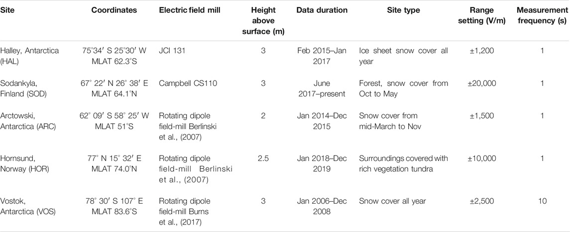
TABLE 1. Details of the high latitude stations and instrumentation used to measure PG.

Figure 1A shows a map of the measurement sites discussed in this paper, demonstrating the high latitude nature of the locations. Examples of the electric field mill sensors used to make the PG measurements are shown in Figures 1B,C for Halley and Sodankyla stations, respectively.

FIGURE 1

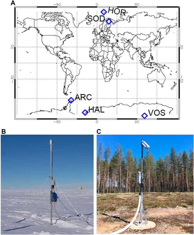
FIGURE 1. (A) Map showing location of high latitude measurement sites described in the paper (denoted by blue diamonds). HOR, Hornsund, SOD, Sodankyla Geophysical Observatory, ARC, Arctowski, HAL, Halley, VOS, Vostok. Photo showing electric field mill at (B) Halley, and (C) Sodankyla.

Details of the various sites are now discussed, with a particular focus on Halley and Sodankyla, as these are not discussed elsewhere in the literature. The British Antarctic Survey Research station Halley VI (75°34′S, 25°30′W) is located on the Brunt Ice Shelf, in Antarctica, approximately 50 km from the coast. Halley is snow covered all year round, with a temperature range from −56° to +1°C, and annual snowfall of approximately 1.2 m. From January 2015 to January 2017 a JCI 131 electric field mill was installed on a 3 m mast approximately 1 km to the south west of the main station buildings. The only structure within 300 m of the field mill was a metal staging caboose (10 × 5 × 8 m high and 30 m from the field mill), which provided shelter for a logging PC and mains power infrastructure. The range of operation of the field mill was restricted to ±1200 V/m to focus on the fair weather range. A full array of meteorological sensors (including temperature, wind, RH, pressure, visibility, ceilometer, solar radiation) were operated at the main research base, ∼1 km from the field mill.

The Sodankyla Geophysical Observatory (67° 22′N, 26° 38′E) is located in northern Finland, within the Arctic circle. The site is in a remote area within a forest, with the town of Sodankyla (population 9,000) being the only inhabited area at about 7 km from the observatory. The lack of human activity in the surrounding area means that sources of man-made pollution at Sodankyla are very low. Temperatures range from −32°C during winter (with snow cover from October to May) to +32°C in summer. A Campbell Scientific CS110 electric field mill was installed on a 3 m mast within a 50 m clearing in the forest from June 2017 to present. A full array of meteorological sensors (including temperature, wind, RH, pressure, visibility, ceilometer, solar radiation) are operated in the meteorological enclosure (near the sounding station), 350 m from the field mill.

A detailed description of site locations for Vostok, Hornsund and Arctowski stations are described in previous works, therefore we only provide a brief description here. Vostok station (78° 30′S, 107°E) is located on the Antarctic plateau, at a height of 3,489 m above sea level (Burns et al., 2005). Hornsund station (77°N, 15° 32′E) is located in the Svalbard archipelago in Norway. It is surrounded by tundra vegetation (Kubicki et al., 2016). Arctowski station (62° 09′S, 58° 25′W) is located in the Southern Shetland Islands, on King George Island. The weather conditions are modulated by the maritime climate zone of the Antarctic (Kubicki et al., 2016).

Summary of PG Data from New Sites and Fair Weather Definitions

Figure 2 shows the time series of PG hourly measurements for Sodankyla (SOD, Figure 2A) and Halley (HAL, Figure 2C) stations. Additionally, the distribution of PG hourly values for both stations is shown in Figures 2B,D for Sodankyla and Halley, respectively. The median PG values are similar between the two sites (SOD = 69 V/m and HAL = 67 V/m), however, the PG variability is very different. This difference in variability is associated with the different meteorological conditions at each site. At Sodankyla, the highest variability is during spring and summer months, when liquid precipitation is common, causing large negative spikes in PG. During the winter, precipitation is mostly snowfall, which tends to produce mainly positive spikes in PG, hence the variability is smallest during these months. At Halley, the variability is quite different, with no obvious seasonal dependence. The extremely low temperatures at Halley all year round mean that there is very little (if any) liquid precipitation, only snowfall, hence the lack of negative spikes in PG at Halley. The few negative PG values here are likely related to blowing snow events. The source of the high variability in PG at Halley is mostly due to high wind speeds and freezing fog events.

FIGURE 2

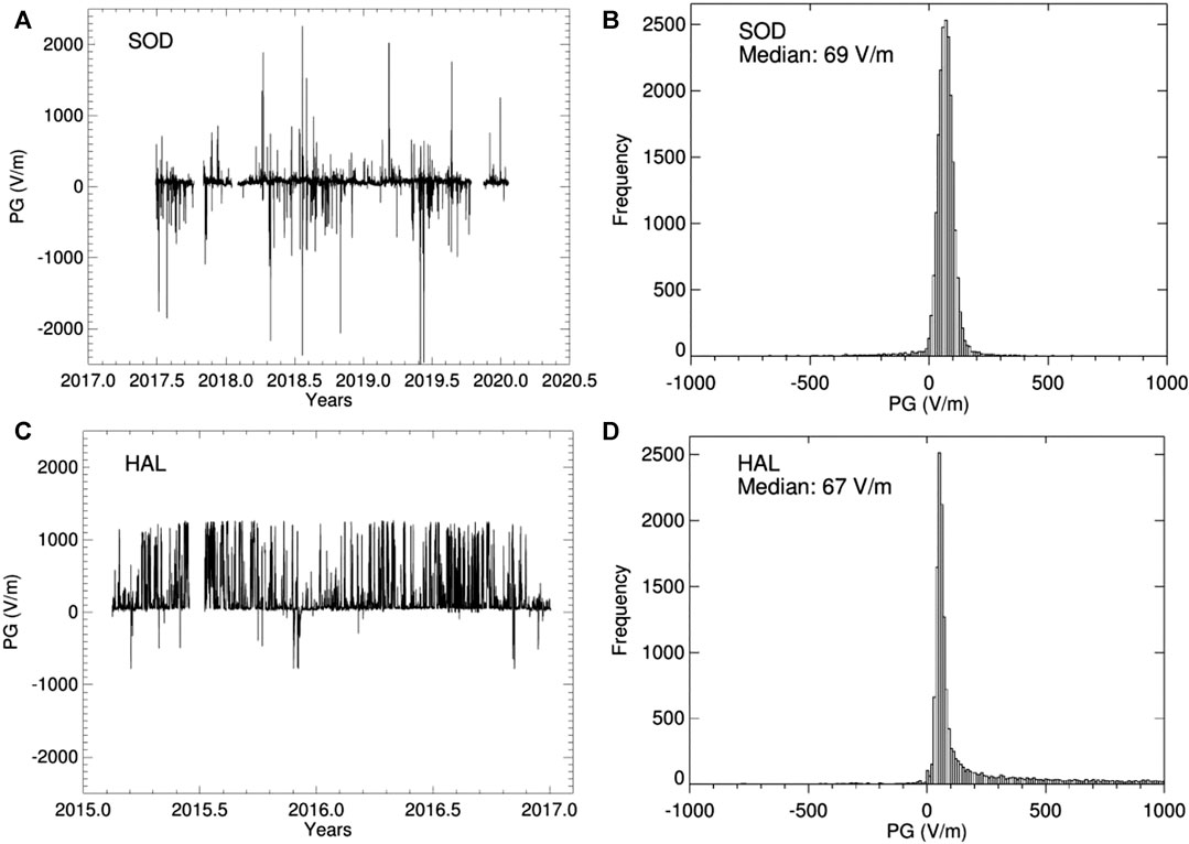
FIGURE 2. Times series of PG for (A) Sodankyla, SOD, and (C) Halley, HAL, stations. PG histogram for (B) SOD and (D) HAL stations, for hourly mean values and plotted within a range of ±1000 V/m.

In order to study GEC signals, it is first necessary to remove any unwanted local effects, such as from meteorological influences, so that only “fair weather” conditions are studied. Although publications exist in the literature regarding the typical definition of fair weather conditions, (e.g., Harrison and Nicoll, 2018) these are generally only for measurement sites where suspended material (such as dust or snow) is unlikely. The criteria specified in Harrison and Nicoll (2018) for fair weather is as follows: absence of hydrometeors, aerosol and haze (with visibility >2 km), negligible cumuliform cloud and no extensive stratus cloud with cloud base below 1,500 m, and surface wind speed between 1 and 8 m/s. Here we briefly examine whether these visibility and wind speed definitions of fair weather are applicable to sites with considerable snow cover, which is typically the case at high latitude sites. Previous research (eg, Simpson, 1921; Currie and Pearce, 1949) has demonstrated that blowing snow particles can become highly charged, thought to be from tribolelectrification and contact charging. Observations have demonstrated that larger particles charge positively and smaller ones negatively (Latham and Stow, 1965), and the movement of these oppositely charged particles can give rise to large PGs of order kV/m.

It is generally accepted (as is the case for sand and dust), that there is a threshold value of wind speed above which snow particles become lifted (e.g., Bagnold, 1941). This is a function of how tightly bonded to the surface the snow particles are, and can depend on snow surface temperature, age of snow, length of duration of high wind speed before the wind event, and many other factors (Li and Pomeroy, 1997). The variability associated with defining a threshold wind speed for blowing snow is demonstrated by Burns et al. (1995) who observed an erratic relationship between PG and wind speed at Davis, Antarctica, where the threshold wind speed value varied between 2 and 14 m/s during individual blowing snow events, and was found to depend on near surface relative humidity (RH). Other values quoted in the literature include 6 m/s for Hornsund and Arctowski (Kubicki et al., 2016), and 10 m/s for Maitri (Panneerselvam et al., 2007). To examine the threshold wind speed for Halley, Figure 3A shows PG plotted against wind speed for 10 min average data for the entire duration of the dataset (31 months). A clear relationship exists between positive values of PG and wind speed for wind speeds above ∼3 m/s, where the PG increases approximately linearly as wind speed increases. The PG is primarily positive until the wind speed reaches 5 m/s, when negative values also start to occur. At wind speeds lower than 3 m/s, the PG is typically <300 V/m, indicating mostly fair weather values. The cluster of large PG values at very low wind speeds (<1 m/s) is likely to be indicative of fog conditions. It should be noted that the maximum range of the field mill at Halley was only ± 1200 V/m, therefore it is very likely that much larger values of PG existed, but were not measured. Figure 3B shows a similar analysis for Sodankyla during months when snow was present on the ground (defined here as snow depth > 2 cm). Very different behavior is apparent, with no clear relationship between PG and wind speed, other than the PG values are mostly fair weather values at wind speeds <2 m/s. The difference in behavior between the two sites is likely related to the fetch of the sites (i.e., the distance upstream of a measurement site that is relatively uniform). At Sodankyla the fetch is small due to the forest location and presence of trees, limiting the transport of snow when it is lofted, whereas Halley is a completely open site, on a smooth, uniform ice sheet, with a long undisturbed fetch. We therefore conclude that the threshold wind speed for blowing snow electrification effects on PG is very much site dependent. At snow covered sites where there is a long fetch, blowing snow has a significant impact on PG, which is likely to start at wind speeds as low as ∼3 m/s.

FIGURE 3

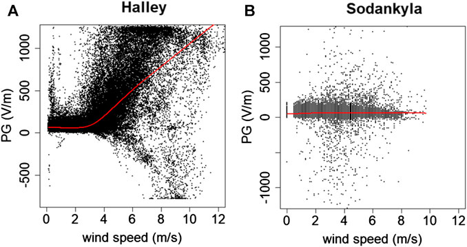
FIGURE 3. Relationship between PG and wind speed at (A) Halley, for the entire duration of the data set, and at (B) Sodankyla when snow depth was >2 cm. Each point is a 10 min average value and the red line represents a lowess fit to the data.

The second fair weather criterion which warrants detailed investigation at high latitude sites is visibility. PG is incredibly sensitive to the presence of aerosol particles or droplets in the air, which generally act to decrease the conductivity. Under conditions of constant vertical conduction current, this leads to an increase in PG, through Ohm’s law. Visibility measurements provide a simple way to detect the presence of such particles by optical means, and can be made automatically using a transmissometer or present weather sensor. Harrison and Nicoll (2018) define fair weather as conditions of “no aerosol or haze, with visibility >2 km”. The 2 km visibility comes from theoretical considerations (Harrison, 2012) which suggest that when aerosol particles are present in low concentration there are large visibilities and little effect on the ambient PG.

Figure 4A shows the relationship between PG and visibility measured at Halley for the entire dataset, which demonstrates that there are obvious clusters of data points in certain areas of the plot. Figure 4B demonstrates that the reason for the clustering in Figure 4A, is that the relationship between PG and visibility is highly dependent on the wind speed, where Figure 4B classifies the data according to low (<2 m/s, gray), medium (between 2 and 7 m/s, blue) and high (>7 m/s, red) wind speeds. From Figure 4B, the red points demonstrate that the highest wind speeds produce the lowest visibility values, and largest magnitude of PG values (including both positive and negative polarities), which are likely to be associated with blowing snow events and snow storms. Low wind speeds (gray points) tend to produce a narrow distribution of PG values, generally between 0–300 V/m (i.e., fair weather values), particularly for visibility >40 km, therefore a combination of wind speed and visibility measurements can assist in the determination of electrically quiescent conditions in snow covered environments. At Halley we therefore use the combination of wind speed <5 m/s (which is increased from the very strict threshold value of 3 m/s to allow more possible PG values), and visibility >40 km to define fair weather periods. The fair weather criteria implemented at each of the other high latitude sites discussed in this paper, as well as the number of fair weather days produced using these criteria is summarised in Table 2. At Sodankyla, the visibility is much more dependent on weather conditions rather than wind speed, so we use the more “traditional” fair weather criteria of cloud cover amount <3/8, wind speed 1 > 6 m/s, no rain precipitation, and visibility range >40 km. For Hornsund and Arctowski stations, fair weather days were chosen with low cloudiness (<4/8), no rain precipitation, drizzle, snow, hail, fog, and wind speed less than 6 m/s (as stated in Kubicki et al., 2016). On the other hand, for Vostok station, where the meteorological data is not easily available, we base our criteria for fair weather days only on the hourly PG variation, which should be between 0–300 V/m. For Hornsund, Arctowski and Vostok, a fair weather day consists of all 24 h PG values meeting the fair weather criteria; whilst for Halley and Sodankyla, at least 20 h must satisfy the criteria. The location of these high latitude sites also means that there is a possibility of unwanted solar effects on the fair weather PG days, therefore we exclude fair weather days where the geomagnetic Kp index was ≥5.

FIGURE 4

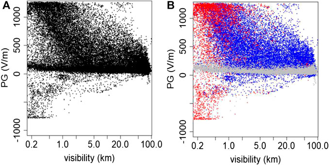
FIGURE 4. (A) Relationship between PG and visibility at Halley (B) colored according to high wind speed conditions (red, wind speed >7 m/s), medium wind speed (blue, wind speed between 2 and 7 m/s), and low wind speed conditions (gray, wind speed <2 m/s). Each point is a 10 min average value.

TABLE 2

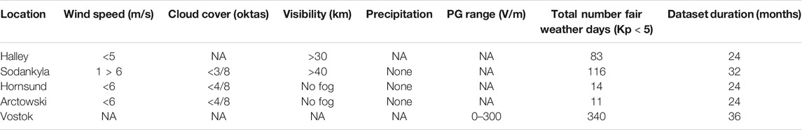
TABLE 2. Summary of criteria used to define fair weather conditions at each of the high latitude sites, and the total number of days on which fair weather was detected. Days on which the geomagnetic Kp index was ≥5 were excluded.

Ionospheric Potential Contributions

PG measurements performed at high latitudes (above 60° magnetic latitude) are influenced by the cross-polar-cap potential difference (Park, 1976b; Burns et al., 2012). When looking at diurnal variations in PG, this manifests itself as a superimposed signal on top of the expected Carnegie diurnal variation, and can be removed by careful analysis. From Table 1, all stations analyzed in this work are above 60° magnetic latitude (except Arctowski station), therefore, if GEC signals are to be considered, it is important to calculate the influence of the polar cap for each site. Following the results from Corney et al. (2003) and Burns et al. (2005), here we use the Weimer model to estimate the cross-polar-cap potential difference. The Weimer model derives the cross-polar-cap potential difference from the combination of the interplanetary magnetic field magnitude (B_z and B_y), solar wind velocity, proton number density and dipole tilt angle (Weimer, 1996; Weimer, 2005). Figure 5 shows the potential difference above Vostok (VOS), Halley (HAL), Hornsund (HOR), and Sodankyla (SOD) stations calculated using the Weimer model (Weimer, 2019). The solid black line represents the mean daily variation and the points are the individual daily hours. The data period used was according to the availability of the PG data (eg, for Halley station the data period was between January 2015 and December 2016). Figure 5 demonstrates that there is a significant effect of the cross-polar-cap potential difference above Vostok (MLAT: 83.6°S) and Hornsund (MLAT: 74°N) stations. There is a variation of 0 to −15 kV above Vostok station with a minimum peak at 19–20 UT. This is in agreement with previous results (Corney et al., 2003; Burns et al., 2005). For Hornsund station, there is a mean daily variation of about ±20 kV where the maximum peak is about 23–02 UT and the minimum peak around 16–17 UT. For the lower magnetic latitude stations of Halley (MLAT: 62.3°S) and Sodankyla (MLAT: 64.1°N) stations, there is much less of an effect of the cross-polar cap potential. For Halley station there is a potential difference in the mean average of less than ±5 kV between 1–4 UT and between 20–24 UT. For the rest of the day, this value is almost zero. In the same way, for Sodankyla station a variation of less than ±5 kV is observed between 16–24 UT. For other hours the values are almost zero.

FIGURE 5

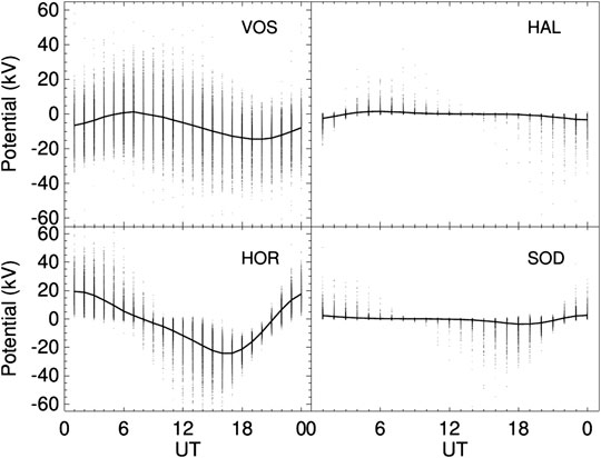
FIGURE 5. Weimer model predictions of the high-latitude electric potentials for VOS (MLAT: 83.6°S; period: 2006–2008), HAL (MLAT: 62.3°S; period: 2015–2016), HOR (MLAT: 74.0°N; period: 2017–2019) and SOD (MLAT: 64.1°N; period: 2017–2019). The points are the individual hours and the solid line is the average value.

To examine what magnitude of effect the cross-polar-cap potential difference has on the measured PG values at the surface, the methodology described by Burns et al. (2005) is employed. First, the average diurnal variation must be removed from the PG, and ionospheric potential values separately. This is done as follows: ΔPG = PG (h) − PG_mean (h); and ΔPotential = Potential (h) − Potential_mean (h). PG (h) and Potential (h) are the hourly averaged PG and the potential difference, respectively, and PG_mean (h) and Potential_mean (h) are the monthly averages for each hour. For Hornsund station, the annual averages were used instead of the monthly averages, due to too few fair weather days to calculate the monthly averages (see Table 2). Following this process, linear regressions were calculated between ΔPG and ΔPotential to determine how closely linked the two variables were. For Vostok and Hornsund stations, all 24 hourly values were used. However, for Halley and Sodankyla stations we consider only 1–4 and 20–24 UT and 15–24 UT, respectively, since Figure 5 indicates a relationship between ΔPG and ΔPotential for only those certain hours of the day. The results are shown in Figure 6 for each station. The scatter in the plots could be associated with the hour to hour variability in the global electric circuit and/or movement of space charge influencing the surface electric conductivity (and therefore the ΔPG), which should not be correlated with the ionospheric potential (ΔPotential). Thus, we observe very low correlation coefficients. A similar effect is mentioned in more detail in Burns et al. (2005).

FIGURE 6

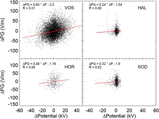
FIGURE 6. Linear regression analysis of the variation from the mean of the vertical electrical field values and the Weimer model inferred cross polar cap potential difference above VOS, HAL, HOR, and SOD. Here, R indicates the Pearson correlation coefficient.

The ratios of ΔPG/ΔPotential for each of the sites are presented in Table 3, and range from 0.24 ± 0.13 V/m per kV for Halley, to 0.60 ± 0.03 V/m per kV for Vostok. Note that the ratio increases as the magnetic latitude of each station increases, as expected due to the influence of the interplanetary magnetic field and the solar wind (important parameters for the Weimer model) that is larger at higher magnetic latitudes. The above calculated ratios from Figure 6 can now be applied to the expected variation in ΔPotential shown in Figure 5, to give final estimates of the effect of the cross-polar-cap potential on the surface PG at the various sites. Applying the maximum calculated variation in ΔPotential of ± 5 kV (from Figure 5) expected at Halley, produces only a very small variation in surface PG of 1.2 V/m. For a similar ΔPotential of ± 5 kV at Sodankyla, this produces a variation of 1.6 V/m. This is comparable to the error in the electric field mill measurements (which is typically ± 1 V/m), and therefore we conclude that on average, cross-polar-cap potential effects are negligible at Halley and Sodankyla. It is noted that the linear fit applied in Figure 6 is not particularly valid for Halley or Sodankyla, but it is included here to demonstrate that there is little effect of ΔPotential on ΔPG. In contrast to the small effects observed at Halley and Sodankyla, for Hornsund and Vostok stations, a potential difference of ∼20 kV should produce a variation of 9.6 and 12 V/m, respectively. These are an order of magnitude larger than those values at lower magnetic latitude stations and approximately 3% of the mean value of PG at Hornsund, and 6% at Vostok. Therefore cross-polar-cap potential effects should be taken into account when analyzing GEC signals at Hornsund and Vostok locations. It should be noted that the analysis performed here is only representative of the average magnetic field conditions. During periods of high magnetic activity there may well be noticeable effects of ΔPotential on the surface PG at Halley and Sodankyla, but this analysis of such effects is out with the scope of the present paper.

TABLE 3

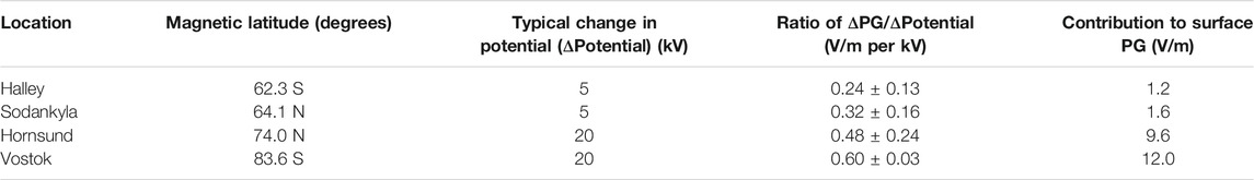
TABLE 3. Summary of effect of cross-polar-cap potential differences at various high latitude sites.

Diurnal Variations

Once the effect of local meteorological influences and ionospheric potential changes has been taken into account it then becomes possible to examine global signals in surface PG data. Figure 7 shows the mean diurnal variation in PG during fair weather at Halley and Sodankyla, separated according to season of the year. At both sites, the characteristic “Carnegie” curve, which represents the total global electrically active generators of the GEC, is apparent, with a minimum in the early morning hours (∼03 UT), and maximum in the evening (∼20 UT). At Sodankyla, Figure 7A, there is a second morning peak around 09 UT during the summer and autumn months. This is consistent with other sites [e g., Mitzpe Ramon, Israel (Yaniv et al., 2016); Reading, United Kingdom (Nicoll et al., 2019)], which display a second morning peak during the convectively active months. The more quiescent meteorological conditions during the winter months (particularly during the polar night) results in a more regular diurnal variation in PG, and the disappearance of the morning maximum peak. At Halley, Figure 7B, there is no morning peak during any of the seasons.

FIGURE 7

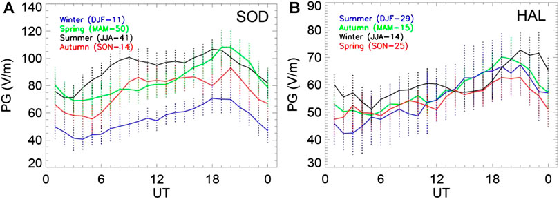
FIGURE 7. Mean diurnal variation in PG for fair weather conditions as a function of season for (A) SOD and (B) HAL stations. The error bars are one standard deviation, and the legend gives the months as well as the number of points included for each season of the year.

At Halley, the average magnitude of the PG variation is similar during all seasons, but markedly lower at Sodankyla during the winter months compared to summer. This seasonal cycle in PG at Sodankyla can also be observed in the time series of PG measurements in Figure 8A. The winter minimum in PG at Sodankyla is likely to be a combination of two factors which can influence the near surface air conductivity, and thus the PG—a minimum in aerosol concentration, and maximum in radon concentration during the winter months. The existence of a seasonal cycle in aerosol at Sodankyla is evidenced by measurements of the columnar property of Aerosol Optical Depth (AOD). Although the AOD is very low at Sodankyla (typically <0.1 at 500 nm, meaning that this an effectively “clean” site), the AOD does minimize during the winter months, and maximize in the summer (Toledano et al., 2012). This seasonality is also observed in surface measurements of aerosol particle concentration from the relatively nearby site at Pallas, Finland, where in spring and summer the daily averages can exceed over 3,000 cm⁻³, but in winter the daily averages decrease to 100 cm⁻³ (Hattaka et al., 2003). The higher aerosol concentrations in the summer months may act to decrease the conductivity, and increase the PG. At Halley, there is also a seasonal cycle in aerosol, which maximizes during the summer months, but even during this maximum period, aerosol concentrations are extremely low (121–179 cm⁻³ during the year 2015) (Lachlan-Cope et al., 2020), and therefore unlikely to have any noticeable effect on the conductivity and PG. The second factor contributing to lower PG values at Sodankyla in the winter months is the increased ionisation due to a seasonal variation in radon concentration. Radon emission depends on properties of the soil (such as temperature, moisture content), as well as meteorological variables controlling mixing processes in the boundary layer (e.g., Singh et al., 1988). Surface measurements of radon concentration from Pallas (Hattaka et al., 2003) demonstrate that radon emission maximizes in November and December, primarily due to stable boundary layer conditions. As the snow depth increases in late winter/early spring, this decreases the radon exhalation rate. The minimum in radon occurs during the summer months when convective mixing is active. We therefore conclude that the combination of low aerosol concentration, and increased ionisation from the high radon concentrations is therefore likely to reduce the PG at Sodankyla during the winter months. It therefore follows that, of the two new high latitude sites presented here, Halley provides more consistently globally representative PG data for GEC studies.

FIGURE 8

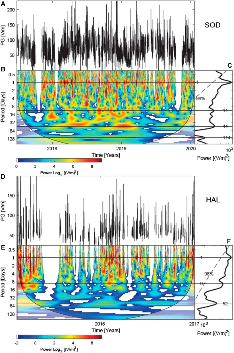
FIGURE 8. Wavelet analysis for SOD and HAL stations. (A,D) Hourly average of the PG amplitude. Gaps are missing data. (B,E) Contours in the time–period domain of the real part of the wavelet power spectra of PG. The contour colors indicate the minimum and maximum magnitude, from blue to red, of the matches between the phases of the time series and the wavelet. The white shadowed lateral edges are values within the cone of influence. (C,F) The global wavelet power spectrum. The horizontal lines indicate the most significant oscillations and the dashed curve is the 98% confidence.

Spectral Analysis

In order to determine whether any regular short term oscillations are present in the new datasets from Halley and Sodankyla, spectral analysis methods are now employed. Wavelet analysis is one of the tools used to retrieve from a time series both the dominant modes and how those modes vary in time (Torrence and Compo, 1998). This study employs the continuous wavelet transform toolbox for MATLAB package (Grinsted et al., 2004), together with a Morlet mother function with frequency w₀ = 6 and a number of voices per power of two equal to 8. Figure 8 shows the wavelet analysis for Sodankyla (A, B, C) and Halley (D, E, F) using PG hourly amplitudes for their entire dataset duration. Figures 8A,D show the time series, where data gaps correspond to periods of no power supply or when there are no fair weather days. To apply the wavelet analysis, constant time steps between samples is required. Such gaps were filled using the moving average of the original time series with a time window length of 3,072 h for both Sodankyla and Halley. This procedure minimizes the introduction of artifacts in the wavelet analysis (Macotela et al., 2019).

Figures 8B,E show the continuous wavelet power spectra corrected by their scales. This correction is employed to rectify the wavelet spectrum, which is biased in favor of larger periods (Liu et al., 2007). The contours represent the magnitude of the matches between the phases of the time series and the wavelet. The color bar indicates the amplitude of those contours that changes from blue to red. The black curves are the cone of influence. The values below this curve must be evaluated with caution. Figures 8C,F show the global wavelet power spectra for Sodankyla and Halley, respectively. The dashed line is their 98% confidence level for a white noise background level. Powers above this line are regarded as significant, whose maxima are indicated by horizontal lines.

Figure 8 shows that the significant oscillations are 1-, 9–11-, 44–52-, and 114-days oscillations. In this study we concentrate on the common periods found for Sodankyla and Halley. Thus, we disregard the 114-day period since it was only observed for Sodankyla, and the resolution at this timescale is low due to the short length of the datasets. The 1-day oscillation can be interpreted as the diurnal Carnegie oscillation and is the most significant oscillation in both time series (Figures 8C,F). This oscillation is much better observed in the periodogram for Sodankyla (Figure 8B), where it is clearest during the winter months. This observation is consistent with Figure 7A, which demonstrates that the strongest link with the single peak Carnegie curve is during the winter season.

In order to confirm our findings, we also performed the Lomb-Scargle periodogram, which allows the analysis of a time series with irregular time steps between samples. Figure 9 shows the Lomb-Scargle periodogram of PG hourly values for Sodankyla (black dotted curve) and Halley (red continuous curve) with normalized power with respect to its value for the 1-day period. The 98% confidence levels are indicated by the red and black horizontal lines for Halley and Sodankyla, respectively. The most significant oscillations found by the wavelet analysis are also indicated by the blue and magenta vertical lines. The 0.5- and 1-day periods are significant in both time series in Figure 9, despite the 0.5 day period not being significant in the wavelet analysis at Halley. This 0.5-day periodicity in PG has been observed at other, more populated mid latitude sites (e.g., Silva et al., 2014), and is generally attributed to diurnal changes in boundary layer conditions, coupled with variations in local sources of pollution (such as traffic), which is more likely to be the case at Sodankyla than Halley.

FIGURE 9

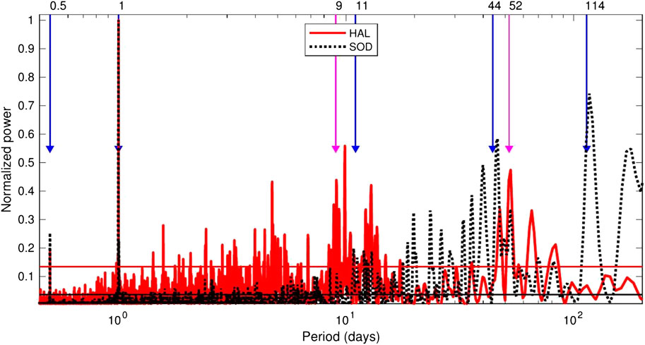
FIGURE 9. Normalized Lomb-Scargle periodogram of PG hourly values for SOD (black dotted curve) and HAL (red continuous curve) stations. The black and red horizontal lines are the 98% significant levels, and the blue and magenta vertical lines are the significant oscillations found by the wavelet analysis for SOD and HAL, respectively. For the 0.5- and 1-day periods the blue and magenta curve are superposed.

The 1-day period is the well-known diurnal oscillation and its observation is expected. The 9–11 and 44–52-days oscillations are not well reported in the literature in PG, if at all. Bennett (2007) reports an 11-day periodicity in PG, air-Earth conduction current (Jc) and near surface conductivity at Reading, United Kingdom, from 14 months of data during 2006–2007, but does not conclude the origin of the periodicity. However, detailed spectral analysis of PG data from Argentina (Tacza et al., 2021) and Portugal (Silva et al., 2014), do not find evidence of these additional periodicities. To further test whether such periodicities are more common at high latitude sites, wavelet analysis was also performed on the PG data from Vostok station (figure not shown here), and 10- and 48-days oscillations were observed, as for Halley and Sodankyla.

It is likely that the sources of the 9–11- and 44–52-days oscillations are related to either local meteorological influences, or variations in ionisation rates [either from oscillations in radon concentration, or Galactic Cosmic Rays (GCRs)]. As there is effectively no radon emission at Halley (as the site location is on a ∼1 km thick ice sheet), this is an unlikely explanation for the observed periodicities. We therefore investigate whether a relationship in the time-period domain exists between the PG and local meteorological measurements (for SOD), as indicated by Macotela et al. (2019). This involves employing the wavelet coherence and cross-wavelet transform. The wavelet coherence is used to measure the degree of local correlation of two series in the time-period domain, while the cross-wavelet transform is employed to find regions in the time-period domain where two time series show common power. The meteorological measurements used included temperature, relative humidity, horizontal visibility, wind direction, and wind speed. Results indicated that, as expected, horizontal visibility, wind direction and wind speed are related to the PG variability, but it is unclear what the source of such periodicities in meteorological phenomenon is. The remaining possibility which may explain the 9–11 days periodicity in PG is a solar influence. 9-day periodicities have been reported in a variety of solar parameters, including the Interplanetary Magnetic Field (IMF), solar wind speed, and also neutron monitors which detect the nucleonic component of Galactic Cosmic Rays (GCRs) (Singh et al., 2012). The 9-days oscillation is a harmonic of the 27-days solar rotation periodicity (Sabbah and Kudela, 2011). The existence of a 9-day periodicity in PG at Halley, Sodankyla and Vostok may therefore also demonstrate the suitability of high latitude sites for studying solar influences on the GEC, but further work on the source of this periodicity is required. This will be examined more closely in a further publication.

Global Electric Circuit Representation

Figure 10 shows the average diurnal variation in fair weather PG measured by the Carnegie research ship (plotted as a percentage of the mean) and the fair weather PG data from the five high latitude sites discussed in this paper, in order to investigate their suitability for GEC analysis. According to the discussion in Ionospheric Potential Contributions, polar cap contributions to the ionospheric potential have been removed from the data at Vostok and Hornsund, but not from Sodankyla, Halley or Arctowski. Figure 10 shows remarkably good agreement between the benchmark of the Carnegie data and most of the high latitude sites in terms of their percentage variations. At Hornsund the peak to peak variation is considerably smaller than at the other sites, but at Vostok (as reported by Burns et al., 2012) and Halley, it is almost identical to the Carnegie variation. This is in contrast to many mid latitude sites which often exhibit a much smaller variation around the time of the primary maximum, and also have secondary maxima related to local aerosol effects (e.g., Yaniv et al., 2016; Nicoll et al., 2019). The timing of the minima of the curves are all similar (to within an hour of 3 UT), with a slight difference in the timings of the maxima of the curves. At the two northern hemisphere sites of Sodankyla and Hornsund, the maxima is approximately 1 h earlier than the Carnegie maximum (at 20 UT), but similar at Vostok and Halley. This may be related to the geographical position of the sites in relation to the location of most of the thunderstorm generators, with the Antarctic sites being closest to the South American generator.

FIGURE 10

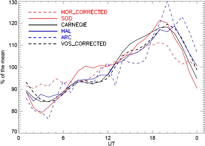
FIGURE 10. Comparison of the PG annual daily variation, in fair weather conditions, between Sodankyla, SOD (red solid line), Hornsund, HOR (red dashed line), Halley, HAL (blue solid line), Arctowski, ARC (blue dashed line), Vostok, VOS (black dashed line) and the Carnegie curve, plotted as percent of the mean. The influence of the cross polar cap potential has been removed for Vostok and Hornsund stations in accordance with the methodology in Ionospheric Potential Contributions.

In terms of the suitability of the various high latitude sites for GEC studies, from those summarised here, the Antarctic sites of Vostok (as previously reported in the literature in various papers by Burns et al.), and Halley are sufficiently unaffected by aerosol sources, and possess a reasonably high proportion of fair weather days to be best suited to GEC research. The influence of the cross-polar-cap potential does affect the PG measurements at Vostok, however, and must be removed, unlike at Halley. The low number of fair weather days at Arctowski on the far northern tip of the Antarctic Peninsula, makes it difficult to assess the suitability of this site, hence further measurements are required. For the Arctic sites, Sodankyla provides a good proportion of fair weather days, but is still subject to local meteorological influences during the spring and summer months. Winter periods do, however, provide good agreement with the GEC oscillation. Finally, Hornsund, with its low number of fair weather days (max. 15–20% in year), and influence of the cross polar cap potential suggests that this is not the easiest of sites to obtain PG measurements for studying global thunderstorm activity, but GEC measurements are possible on individual days.

Conclusion

This paper presents the first analysis of PG data from two new high latitude sites at opposite ends of the Earth - Sodankyla in the Arctic, and Halley in the Antarctic. These new datasets are compared with other existing PG datasets from high latitudes in order to assess their suitability for Global Electric Circuit (GEC) measurements. Detailed analysis of meteorological data at Halley demonstrates the usefulness of visibility data for determination of fair weather conditions at snow covered sites, which is required to indicate globally representative data. A clear relationship between PG and wind speed at Halley is also demonstrated, which shows that snow can be lofted at wind speeds as low as 3 m/s, but also, for the first time, that the threshold wind speed for blowing snow effects on the PG is dependent on the fetch of the measurement site. Spectral analysis of the PG demonstrates 1 day, as well as 9–11 days and 44–52 day periodicities at both sites. Although the 1 day periodicity is expected, the others are less understood, and may be related to variations in local meteorological influences or solar parameters. The influence of cross-polar-cap variations in ionospheric potential is also investigated, and found to be negligible at the two new measurement sites. Comparison of the diurnal variations in PG data from Sodankyla and Halley, with the universal Carnegie curve of the GEC, shows good agreement in terms of the peak to peak oscillations, and timings of the minima and maxima of the curves. Sodankyla displays a secondary morning peak during the summer months, likely related to convective activity, but is in close agreement with the Carnegie GEC variation during the winter months. Comparison of the new data PG from Sodankyla and Halley with other existing high latitude PG datasets from Hornsund (Arctic), Arctowski (Antarctic), and Vostok (Antarctic), confirms the suitability of the continental Antarctic sites, in particular, for GEC measurements. Despite the difficulties associated with maintaining instrumentation in such harsh climatic conditions, the lack of aerosol contamination, and relatively high proportion of fair weather days means that of the high latitude stations studied here, Halley and Vostok provide the most suitable sites for GEC analysis.

Data Availability Statement

Sodankyla PG data are available from KN (k.a.nicoll@reading.ac.uk) at the University of Reading on request. Halley PG data is available from the GloCAEM database hosted by CEDA: http://data.ceda.ac.uk/badc/glocaem/data/halley. Sodankyla meteorological data is available from the LITB database, of the Finnish Meteorological Institute (https://litdb.fmi.fi/). Vostok PG data is available from: Burns et al. (2013). Hornsund and Arctowski PG data are available on request from MK at Swider Geophysical Observatory (swider@igf.edu.pl). Weimer 2005 ionospheric electric potential model was provided by D. Weimer and is available at https://zenodo.org/record/2530324. Solar wind data were obtained from the National Space Science Data Center OMNIWeb database (https://omniweb.gsfc.nasa.gov/form/dx1.html).

Author Contributions

JT and KN contributed to the study designing, data processing, data analysis, data interpreting, and manuscript writing. EM contributed to the spectral analysis and manuscript writing. MK, AO, and JM contributed to the data curation, data processing and data analysis. All authors contributed to the manuscript revision and approved the submitted version.

Funding

KN acknowledges an Independent Research Fellowship funded by the Natural Environment Research Council NERC (NE/L011514/1) and (NE/L011514/2). The Halley PG data was obtained in collaboration with the British Antarctic Survey (with thanks to David Maxfield and Mervyn Freeman) through a NERC Collaborative Gearing Scheme grant, and archived through the GloCAEM project (NERC International Opportunities Fund grant NE/N013689/1). Ilya Usoskin from the University of Oulu, Thomas Ulich and his technical team at Sodankyla Geophysical Observatory were instrumental in obtaining the Sodankyla PG measurements. JT acknowledges the Polish National Agency for Academic Exchange for funding of the Ulam Program scholarship agreement no PPN/ULM/2019/1/00328/U/00001. Observations at Polish Polar Station Hornsund were supported by SPUB grants from Ministry of Science and Higher Education of Poland. The observations at Arctowski Antarctic station of the Institute of Biochemistry and Biophysics, Polish Academy of Sciences, have been financed by National Science Centre grant number NCN-2011/01/B/ST10/07118 (2011–2014) awarded to the Institute of Geophysics, Polish Academy of Sciences.

Conflict of Interest

The authors declare that the research was conducted in the absence of any commercial or financial relationships that could be construed as a potential conflict of interest.

Acknowledgments

JT thanks the Arctic Interactions research profile action of the University of Oulu for making possible his visit to the Sodankyla Geophysical Observatory. Work of MK and AO is financed by Institute of Geophysics, Polish Academy of Sciences, with a subsidy from Poland Ministry of Science and Higher Education (now Ministry of Education and Science). The authors thank the reviewers for their constructive comments and suggestions, which helped to improve the quality of the paper.

Footnotes

¹Potential gradient = −Ez (where Ez is the vertical electric field).

²Fair weather conditions are those in which there is absence of hydrometeors, aerosol and haze, negligible cumuliform cloud and not extensive stratus cloud with cloud base below 1.5 km, and surface wind speed between 1 and 8 m/s (Harrison and Nicoll, 2018).

References

Anisimov, S. V., Galichenko, S. V., Aphinogenov, K. V., and Prokhorchuk, A. A. (2018). Evaluation of the atmospheric boundary-layer electrical variability. Boundary-Layer Meteorol. 167 (2), 327–348.

Google Scholar

Bagnold, R. A. (1941). Electrification of wind-blown sand: recent advances and key issues. Eur. Phys. J. E Soft Matter. 36 (12), 1–15. doi:10.1140/epje/i2013-13138-4

CrossRef Full Text | Google Scholar

Barbosa, S. (2020). Ambient radioactivity and atmospheric electric field: a joint study in an urban environment. J. Environ. Radioact. 219, 106283. doi:10.1016/j.jenvrad.2020.106283

PubMed Abstract | CrossRef Full Text | Google Scholar

Bennett, A. (2007). Measurement of atmospheric electricity during different meteorological conditions. PhD thesis. Reading, UK: University of Reading.

Google Scholar

Berlinski, J., Pankanin, G., and Kubicki, M. (2007). “Large scale monitoring of troposphere electric field,” in Proceedings of the 13th International Conference on Atmospheric Electricity, Beijing, China, August 13–18, 2007 (Beijing: International Conference on Atmospheric Electricity), 124–126.

Google Scholar

Burns, G. B., Hesse, M. H., Parcell, S. K., Malachowski, S., and Cole, K. D. (1995). The geoelectric field at Davis station, Antarctica. J. Atmos. Sol. Terr. Phys. 57 (14), 1783–1797. doi:10.1016/0021-9169(95)00098-m

CrossRef Full Text | Google Scholar

Burns, G. B., Frank-Kamenetski, A. V., Troshichev, O. A., Bering, E. A., and Redell, B. D. (2005). Interannual consistency of bi-monthly differences in diurnal variations of the ground-level, vertical electric field. J. Geophys. Res. 110 (D10), 106. doi:10.1029/2004jd005469

CrossRef Full Text | Google Scholar

Burns, G. B., Tinsley, B. A., Frank-Kamenetski, A. V., Troshichev, O. A., French, W. J. R., and Klekociuk, A. R. (2012). Monthly diurnal global atmospheric circuit estimates derived from Vostok electric field measurements adjusted for local meteorological and solar wind influences. J. Atmos. Sci. 69 (6), 2061–2082. doi:10.1175/jas-d-11-0212.1

CrossRef Full Text | Google Scholar

Burns, G., Tinsley, B., Frank-Kamenetsky, A. V., Troshichev, O., and Bering, E. A. (2013). Vertical Electric Field—Vostok from 2006–2011. Canberra, ACT: Australian Antarctic Data Centre (Accessed September 7 2020). doi:10.4225/15/58880fc1a1fbd

CrossRef Full Text | Google Scholar

Burns, G. B., Frank-Kamenetski, A. V., Tinsley, B. A., French, W. J. R., Grigioni, P., Camporeale, G., et al. (2017). Atmospheric global circuit variations from vostok and concordia electric field measurements. J. Atmos. Sci. 74 (3), 783–800. doi:10.1175/jas-d-16-0159.1

CrossRef Full Text | Google Scholar

Cobb, W. E. (1977). “Atmospheric electric measurements at the south Pole,” in Electrical Processes in Atmospheres. Editors H. Dolezalek, and R. Reiter (Darmstadt, Germany: Steinkopf), 161–167.

Google Scholar

Corney, R. C., Burns, G. B., Michael, K., Frank-Kamenetsky, A. V., Troshichev, O. A., Bering, E. A., et al. (2003). The influence of polar-cap convection on the geoelectric field at Vostok, Antarctica. J. Atmos. Sol. Terr. Phys. 65 (3), 345–354. doi:10.1016/s1364-6826(02)00225-0

CrossRef Full Text | Google Scholar

Currie, B. W., and Pearce, D. C. (1949). Some qualitative results on the electrification of snow. Can. J. Res. 27 (1), 1–8. doi:10.1139/cjr49a-001

CrossRef Full Text | Google Scholar

Fisk, H. W., and Fleming, J. A. (1928). The magnetic and electric observations of the maud expedition during 1918 to 1925. Terr. Magnetism Atmos. Electr. 33 (1), 37–43. doi:10.1029/te033i001p00037

CrossRef Full Text | Google Scholar

Frank-Kamenetsky, A. V., Burns, G. B., Troshichev, O. A., Papitashvili, V. O., Bering, E. A., and French, W. J. R. (1999). The geoelectric field at Vostok, Antarctica: its relation to the interplanetary magnetic field and the cross polar cap potential difference. J. Atmos. Sol. Terr. Phys. 61 (18), 1347–1356. doi:10.1016/s1364-6826(99)00089-9

CrossRef Full Text | Google Scholar

Grinsted, A., Moore, J. C., and Jevrejeva, S. (2004). Application of the cross wavelet transform and wavelet coherence to geophysical time series. Nonlinear Process. Geophys. 11 (5–6), 561–566. doi:10.5194/npg-11-561-2004

CrossRef Full Text | Google Scholar

Hairston, M. R., and Heelis, R. A. (1990). Model of the high latitude ionospheric convection pattern during southward interplanetary magnetic field using DE-2 data. J. Geophys. Res. 95 (A3), 2333–2343. doi:10.1029/ja095ia03p02333

CrossRef Full Text | Google Scholar

Haldoupis, C., Rycroft, M., Williams, E., and Price, C. (2017). Is the “earth-ionosphere capacitor” a valid component in the atmospheric electric circuit?. J. Atmos. Sol. Terr. Phys. 164, 127–131. doi:10.1016/j.jastp.2017.08.012

CrossRef Full Text | Google Scholar

Harrison, R. G. (2012). Aerosol-induced correlation between visibility and atmospheric electricity. J. Aerosol Sci. 52, 121–126. doi:10.1016/j.jaerosci.2012.04.011

CrossRef Full Text | Google Scholar

Harrison, R. G., and Aplin, K. L. (2002). Mid-nineteenth century smoke concentrations near London. Atmos. Env. 36, 4037–4043.

Harrison, R. G., and Nicoll, K. A. (2018). Fair weather criteria for atmospheric electricity measurements. J. Atmos. Sol. Terr. Phys. 179, 239–250. doi:10.1016/j.jastp.2018.07.008

CrossRef Full Text | Google Scholar

Harrison, R. G. (2013). The Carnegie curve. Surv. Geophys. 34 (2), 209–232. doi:10.1007/s10712-012-9210-2

CrossRef Full Text | Google Scholar

Hatakka, J., Aalto, T., Aaltonen, V., Aurela, M., Hakola, H., Komppula, M., et al. (2003). Overview of the atmospheric research activities and results at Pallas GAW station. Boreal Environ. Res. 8 (4), 365–384

Google Scholar

Jeeva, K., Gurubaran, S., Williams, E. R., Kamra, A. K., Sinha, A. K., Guha, A., et al. (2016). Anomalous diurnal variation of atmospheric potential gradient and air-earth current density observed at Maitri, Antarctica. J. Geophys. Res. Atmos. 121 (21), 12593–12611. doi:10.1002/2016jd025043

CrossRef Full Text | Google Scholar

Kasemir, H. W. (1972). Atmospheric electric measurements in the Arctic and the Antarctic. Pure Appl. Geophys. 100 (1), 70–80. doi:10.1007/bf00880228

CrossRef Full Text | Google Scholar

Kubicki, M., Odzimek, A., and Neska, M. (2016). Relationship of ground-level aerosol concentration and atmospheric electric field at three observation sites in the Arctic, Antarctic and Europe. Atmos. Res. 178–179, 329–346. doi:10.1016/j.atmosres.2016.03.029

PubMed Abstract | CrossRef Full Text | Google Scholar

Lachlan-Cope, T., Beddows, D. C., Brough, N., Jones, A. E., Harrison, R. M., Lupi, A., et al. (2020). On the annual variability of Antarctic aerosol size distributions at Halley research station. Atmos. Chem. Phys. 20 (7), 4461–4476. doi:10.5194/acp-20-4461-2020

CrossRef Full Text | Google Scholar

Latham, J., and Stow, C. D. (1965). The electrification of blowing snow. J. Meteorol. Soc. Jpn. 43 (1), 23–29.

CrossRef Full Text | Google Scholar

Li, L., and Pomeroy, J. W. (1997). Probability of occurrence of blowing snow. J. Geophys. Res. Space Phys. 102 (D18), 21955–21964. doi:10.1029/97jd01522

CrossRef Full Text | Google Scholar

Liu, Y., San Liang, X., and Weisberg, R. H. (2007). Rectification of the bias in the wavelet power spectrum. J. Atmos. Ocean. Technol. 24 (12), 2093–2102. doi:10.1175/2007jtecho511.1

CrossRef Full Text | Google Scholar

Macotela, E. L., Clilverd, M., Manninen, J., Moffat-Griffin, T., Newnham, D. A., Raita, T., et al. (2019). D-region high-latitude forcing factors. J. Geophys. Res. Space Phys. 124 (1), 765–781. doi:10.1029/2018ja026049

CrossRef Full Text | Google Scholar

Markson, R. (1986). Tropical convection, ionospheric potentials and global circuit variation. Nature 320 (6063), 588–594. doi:10.1038/320588a0

CrossRef Full Text | Google Scholar

Nicoll, K. A., Harrison, R. G., Barta, V., Bor, J., Brugge, R., Chillingarian, A., et al. (2019). A global atmospheric electricity monitoring network for climate and geophysical research. J. Atmos. Sol. Terr. Phys. 184, 18–29. doi:10.1016/j.jastp.2019.01.003

CrossRef Full Text | Google Scholar

Nicoll, K. A., and Harrison, R. G. (2016). Stratiform cloud electrification: comparison of theory with multiple in-cloud measurements. Q. J. R. Meteorol. Soc. 142 (700), 2679–2691. doi:10.1002/qj.2858

CrossRef Full Text | Google Scholar

Odzimek, A. (2019). Polar regions in the global atmospheric electric circuit research, English translation of Obszary polarne w badaniach globalnego atmosferycznego obwodu elektrycznego Ziemi. Przeglad Geofiz. 64 (1–2), 35–72. doi:10.32045/PG-2019-002

CrossRef Full Text | Google Scholar

Panneerselvam, C., Selvaraj, C., Jeeva, K., Nair, K. U., Anilkumar, C. P., and Gurubaran, S. (2007). Fairweather atmospheric electricity at Antarctica during local summer as observed from Indian station, Maitri. J. Earth Syst. Sci. 116 (3), 179–186. doi:10.1007/s12040-007-0018-2

CrossRef Full Text | Google Scholar

Papitashvili, V. O., Belov, B. A., Faermark, D. S., Feldstein, Y. I., Golyshev, S. A., Gromova, L. I., et al. (1994). Electric potential patterns in the northern and southern polar regions parameterized by the interplanetary magnetic field. J. Geophys. Res. 99 (A7), 13251–13262. doi:10.1029/94ja00822

CrossRef Full Text | Google Scholar

Papitashvili, V. O., Clauer, C. R., Levitin, A. R., and Belov, B. A. (1995). Relationship between the observed and modeled modulation of the dayside ionospheric convection by the IMF by component. J. Geophys. Res. 100 (A5), 7715–7722. doi:10.1029/94ja01344

CrossRef Full Text | Google Scholar

Park, C. G. (1976a). Solar magnetic sector effects on the vertical atmospheric electric field at Vostok, Antarctica. Geophys. Res. Lett. 3 (8), 475–478. doi:10.1029/gl003i008p00475

CrossRef Full Text | Google Scholar

Park, C. G. (1976b). Downward mapping of high-latitude ionospheric electric fields to the ground. J. Geophys. Res. 81 (1), 168–174. doi:10.1029/ja081i001p00168

CrossRef Full Text | Google Scholar

Peterson, M., Deierling, W., Liu, C., Mach, D., and Kalb, C. (2017). A TRMM/GPM retrieval of the total generator current for the global electric circuit. J. Geophys. Res.: Atmosphere. 122 (18), 10025–10049. doi:10.1002/2016jd026336

CrossRef Full Text | Google Scholar

Price, C. (1993). Global surface temperatures and the atmospheric electric circuit. Geophys. Res. Lett. 20 (13), 1363–1366. doi:10.1029/93gl01774

CrossRef Full Text | Google Scholar

Rycroft, M. J., Israelsson, S., and Price, C. (2000). The global atmospheric electric circuit, solar activity and climate change. J. Atmos. Sol. Terr. Phys. 62 (17–18), 1563–1576. doi:10.1016/s1364-6826(00)00112-7

CrossRef Full Text | Google Scholar

Rycroft, M. J., Harrison, R. G., Nicoll, K. A., and Mareev, E. A. (2008). An overview of Earth’s global electric circuit and atmospheric conductivity. Space Sci. Rev. 137 (1–4), 83–105. doi:10.1007/s11214-008-9368-6

CrossRef Full Text | Google Scholar

Rycroft, M. J., Nicoll, K. A., Aplin, K. L., and Harrison, R. G. (2012). Recent advances in global electric circuit between the space environment and the troposphere. J. Atmos. Sol. Terr. Phys. 90–91, 198–211. doi:10.1016/j.jastp.2012.03.015

PubMed Abstract | CrossRef Full Text | Google Scholar

Sabbah, I., and Kudela, K. (2011). Third harmonic of the 27 day periodicity of galactic cosmic rays: coupling with interplanetary parameters. J. Geophys. Res. Space Phys. 116 (A4), A04103. doi:10.1029/2010ja015922

CrossRef Full Text | Google Scholar

Silva, H. G., Conceição, R., Melgão, M., Nicoll, K., Mendes, P. B., Tlemçani, M., et al. (2014). Atmospheric electric field measurements in urban environment and the pollutant aerosol weekly dependence. Environ. Res. Lett. 9, 114025.

Simpson, G. C. (1905). Atmospheric electricity in high latitudes. Proc. R. Soc. A. 76 (508), 61–97. doi:10.1098/rspa.1905.0014

CrossRef Full Text | Google Scholar

Simpson, G. C. (1919). British antarctic expedition, 1910–1913: Meteorology. (Calcutta, India: Thacker, Spink and Co.), Vol. 1.

Google Scholar

Simpson, G. C. (1921). “Atmospheric electricity,” in British antarctic exp. 1910–1913. (London, United Kingdom: Har-rison and Sons), Vol. 1

Google Scholar

Singh, M., Ramola, R. C., Singh, S., and Virk, H. S. (1988). The influence of meteorological parameters on soil gas radon. J. Assoc. Explor. Geophys. 9, 85–90.

Google Scholar

Singh, Y. P., and Gautam, S. (2012). Temporal variations of short-and mid-term periodicities in solar wind parameters and cosmic ray intensity. J. Atmos. Sol. Terr. Phys. 89, 48–53. doi:10.1016/j.jastp.2012.07.011

CrossRef Full Text | Google Scholar

Tacza, J., Raulin, J.-P., Macotela, E., Marun, A., Fernandez, G., Bertoni, F., et al. (2020). Local and global effects on the diurnal variation of the atmospheric electric field in South America by comparison with the carnegie curve. Atmos. Res. 240, 104938. doi:10.1016/j.atmosres.2020.104938

CrossRef Full Text | Google Scholar

Tacza, J., Raulin, J.-P., Morales, C. A., Macotela, E., Marun, A., and Fernandez, G. (2021). Analysis of long-term potential gradient variations measured in the argentinian andes. Atmos. Res. 248, 105200. doi:10.1016/j.atmosres.2020.105200

CrossRef Full Text | Google Scholar

Tinsley, B. A., Burns, G. B., and Zhou, L. (2007). The role of the global electric circuit in solar and internal forcing of clouds and climate. Adv. Space Res. 40 (7), 1126–1139. doi:10.1016/j.asr.2007.01.071

CrossRef Full Text | Google Scholar

Tinsley, B. A., Liu, W., Rohrbaugh, R. P., and Kirkland, M. W. (1998). South pole electric field responses to overhead ionospheric convection. J. Geophys. Res. 103 (D20), 26137–26146. doi:10.1029/98jd02646

CrossRef Full Text | Google Scholar

Toledano, C., Cachorro, V. E., Gausa, M., Stebel, K., Aaltonen, V., Berjón, A., et al. (2012). Overview of sun photometer measurements of aerosol properties in Scandinavia and Svalbard. Atmos. Environ. 52, 18–28. doi:10.1016/j.atmosenv.2011.10.022

CrossRef Full Text | Google Scholar

Torrence, C., and Compo, G. (1998). A practical guide to wavelet analysis. Bull. Am. Meteorol. Soc. 79 (1), 61–78. doi:10.1175/1520-0477(1998)079<0061:apgtwa>2.0.co;2

CrossRef Full Text | Google Scholar

Weimer, D. R. (1995). Models of high-latitude electric potentials derived with a least error fit of spherical harmonic coefficients. J. Geophys. Res. 100, 19595–19607.

Weimer, D. R. (1996). A flexible, IMF dependent model of high-latitude electric potentials having “space weather” applications. Geophys. Res. Lett. 23 (18), 2549–2552. doi:10.1029/96gl02255

CrossRef Full Text | Google Scholar

Weimer, D. R. (2005). Improved ionospheric electrodynamic models and application to calculating Joule heating rates. J. Geophys. Res. 110 (A5), 306. doi:10.1029/2004ja010884

CrossRef Full Text | Google Scholar

Weimer, D. R. (2019). Weimer 2005 ionospheric electric potential model for IDL (Version 2005). J. Geophys. Res. 110, A12307. doi:10.5281/zenodo.2530324

CrossRef Full Text | Google Scholar

Whipple, F. J. W. (1929). On the association of the diurnal variation of electric potential gradient in fine weather with the distribution of thunderstorms over the globe. Q. J. R. Meteorol. Soc. 55 (229), 1–17. doi:10.1002/qj.49705522902

CrossRef Full Text | Google Scholar

Williams, E., and Mareev, E. (2014). Recent progress on the global electric circuit. Atmos. Res. 135–136, 208–227. doi:10.1016/j.atmosres.2013.05.015

PubMed Abstract | CrossRef Full Text | Google Scholar

Williams, E. R. (1992). The Schumann resonance: a global tropical thermometer. Science. 256 (5960), 1184–1187. doi:10.1126/science.256.5060.1184

PubMed Abstract | CrossRef Full Text | Google Scholar

Williams, E. R. (2009). The global electric circuit: a review. Atmos. Res. 91 (2–4), 140–152. doi:10.1016/j.atmosres.2008.05.018

CrossRef Full Text | Google Scholar

Wilson, C. T. R. (1921). Investigations on lightning discharges and on the electric field of thunderstorms. Philos. Trans. Roy. Soc. London. 221 (582–593), 73–115. doi:10.1098/rsta.1921.0003

CrossRef Full Text | Google Scholar

Yaniv, R., Yair, Y., Price, C., and Katz, S. (2016). Local and global impacts on the fair-weather electric field in Israel. Atmos. Res. 172–173, 119–125. doi:10.1016/j.atmosres.2015.12.025

PubMed Abstract | CrossRef Full Text | Google Scholar